Embed Size (px)
Citation preview
10.1098/rspa.2003.1174
Eshelby problem of polygonal inclusions inanisotropic piezoelectric bimaterials
By E. Pan
Department of Civil Engineering, The University of Akron,Akron, OH 44325-3905, USA ([email protected])
Received 3 February 2003; revised 9 April 2003; accepted 23 April 2003;published online 4 December 2003
This paper studies the two-dimensional Eshelby problem in anisotropic piezoelec-tric bimaterials. Assuming that the inclusion is an arbitrarily shaped polygon withuniform eigenstrain and eigenelectric fields, we derive the exact closed-form solu-tion by integrating analytically the line-source Green functions in the correspondingbimaterials. The required line-source Green functions are obtained in terms of theStroh formalism and include six different interface models. Since the induced elasticand piezoelectric fields due to the eigenstrain and eigenelectric fields are given inthe exact closed form in terms of simple elementary functions, those due to multi-ple inclusions can be superposed together. Benchmark numerical examples are alsopresented for the induced elastic and piezoelectric fields within a square inclusiondue to a uniform hydrostatic eigenstrain with the bimaterials being made of typicalquartz and ceramic.
Keywords: Eshelby problem; Green’s function; anisotropic piezoelectric bimaterials;Stroh formalism; imperfect interface; quantum wires
1. Introduction
It is well known that the Eshelby problem (Eshelby 1957, 1959, 1961; Willis 1981;Mura 1987; Dunn & Taya 1993) is fundamental to various engineering and physicalfields, and thus is the subject of continuing studies (Bacon et al . 1978; Mura 1987;Ting 1996; Buryachenko 2001). In recent years, the Eshelby problem of any shapedinclusion has been found to be particularly useful in the study of nanoscale semicon-ductor quantum devices (Gosling & Willis 1995; Faux & Pearson 2000; Glas 2001).The embedded quantum dot (QD) and quantum wire (QWR) can induce large elasticand piezoelectric fields which in turn can have a strong influence on the electronicand optical properties of the semiconductor nanostructures (see, for example, Singh1993; Davies 1998a, b; Bimberg et al . 1999; Ram-Mohan 2002; Freund & Johnson2001; Waltereit et al . 2002). It is further noted that piezoelectric coupling could bean important contribution to the electronic and optical properties of the semicon-ductor structure, due to the fact that most semiconductor materials are piezoelectric(Davies & Larkin 1994; Jogai 2001; Pan 2002a, b; Pan & Yang 2003).
In the study of the Eshelby problem, material anisotropy poses great difficulty.While, for the three-dimensional (3D) case, Yu et al . (1994) derived the solutionfor inclusions in a transversely isotropic and elastic bimaterial space, Ru (2000,
Proc. R. Soc. Lond. A (2004) 460, 537–560537
c© 2003 The Royal Society
538 E. Pan
2001) proposed a conformal mapping solution for an arbitrarily shaped inclusionin an anisotropic piezoelectric full plane, half-plane, or bimaterial full plane, underthe assumption of two-dimensional (2D) deformation. For the purely elastic cubic bi-material full plane, on the other hand, Yu (2001) obtained exact closed-form solutionsfor the Eshelby problem. More recently, the author derived an exact closed-form solu-tion for an arbitrarily shaped polygonal inclusion in an anisotropic piezoelectric fullplane and half-plane (Pan 2004). Until now, however, an exact closed-form solutionof the Eshelby problem in the corresponding anisotropic piezoelectric bimaterial fullplane has still been unavailable in the literature. Yet, such a solution, if obtained inan exact closed form, is very desirable in current nanoscale QWR structure analysisas well as in various engineering and physical fields. Furthermore, the exact closed-form solution to the Eshelby problem can serve directly as the kernel function invarious boundary-integral-equation formulations.
In this paper, we thus present the exact closed-form solution for an arbitrarilyshaped polygonal inclusion in anisotropic piezoelectric bimaterials. We first expressthe induced elastic and piezoelectric fields in terms of a line integral on the bound-ary of the inclusion, based on the equivalent body-force concept of eigenstrain andeigenelectric fields. In the line-integral expression, the integrand is the line-sourceGreen functions of the bimaterials, which have been also derived in this paper for sixdifferent interface models. We then carry out the line integral analytically assumingthat the inclusion is a polygon. The most striking feature is that the final exactclosed-form solution involves only elementary functions. Consequently, the elasticand piezoelectric fields due to multiple inclusions or an array of QWRs can beobtained easily by the superposition method. Furthermore, the induced field dueto an elliptical inclusion can also be obtained by approximating the curvilinear ele-ment on the boundary of the inclusion with the straight-line element. Numericalresults are presented as benchmarks where the inclusion is a square-shaped QWRunder a hydrostatic eigenstrain, with the bimaterials being made of typical quartzand ceramic. We further remark that the present exact closed-form solution for theEshelby problem in anisotropic piezoelectric bimaterials also includes the Eshelbysolution corresponding to the anisotropic elastic bimaterials as a special case, forwhich the exact closed-form solution is also unavailable.
This paper is organized as follows: In § 2, the Eshelby problem in anisotropicpiezoelectric bimaterials is described using shorthand notation. In § 3, we first definethe equivalent body force of the eigenstrain and eigenelectric field, and then derivethe boundary integral expression for the induced elastic and piezoelectric fields interms of the line-source Green functions. In § 4, the exact closed-form solution forthe induced elastic and electric fields due to a polygonal inclusion of arbitrary shapeis derived. While benchmark numerical examples are presented in § 5, certain con-clusions are drawn in § 6. The six different interface models are briefly described inAppendix A, and the related bimaterial Green functions are derived in Appendix B.Finally, the exact closed-form expressions for the line integral of the bimaterial Greenfunctions on the boundary of the inclusion are presented in Appendix C.
2. Description of the Eshelby problem in bimaterial full plane
Consider an anisotropic and piezoelectric bimaterial full-plane (x, z), where z > 0 andz < 0 are occupied by materials 1 and 2, respectively, with the interface being on the
Proc. R. Soc. Lond. A (2004)
Eshelby problem of polygonal inclusions 539
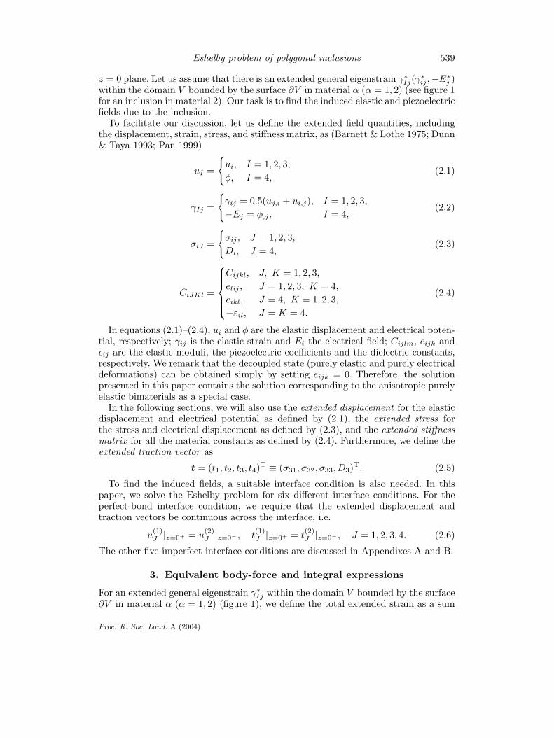
z = 0 plane. Let us assume that there is an extended general eigenstrain γ∗Ij(γ
∗ij , −E∗
j )within the domain V bounded by the surface ∂V in material α (α = 1, 2) (see figure 1for an inclusion in material 2). Our task is to find the induced elastic and piezoelectricfields due to the inclusion.
To facilitate our discussion, let us define the extended field quantities, includingthe displacement, strain, stress, and stiffness matrix, as (Barnett & Lothe 1975; Dunn& Taya 1993; Pan 1999)
uI =
{ui, I = 1, 2, 3,
φ, I = 4,(2.1)
γIj =
{γij = 0.5(uj,i + ui,j), I = 1, 2, 3,
−Ej = φ,j , I = 4,(2.2)
σiJ =
{σij , J = 1, 2, 3,
Di, J = 4,(2.3)
CiJKl =
Cijkl, J, K = 1, 2, 3,
elij , J = 1, 2, 3, K = 4,
eikl, J = 4, K = 1, 2, 3,
−εil, J = K = 4.
(2.4)
In equations (2.1)–(2.4), ui and φ are the elastic displacement and electrical poten-tial, respectively; γij is the elastic strain and Ei the electrical field; Cijlm, eijk andεij are the elastic moduli, the piezoelectric coefficients and the dielectric constants,respectively. We remark that the decoupled state (purely elastic and purely electricaldeformations) can be obtained simply by setting eijk = 0. Therefore, the solutionpresented in this paper contains the solution corresponding to the anisotropic purelyelastic bimaterials as a special case.
In the following sections, we will also use the extended displacement for the elasticdisplacement and electrical potential as defined by (2.1), the extended stress forthe stress and electrical displacement as defined by (2.3), and the extended stiffnessmatrix for all the material constants as defined by (2.4). Furthermore, we define theextended traction vector as
t = (t1, t2, t3, t4)T ≡ (σ31, σ32, σ33, D3)T. (2.5)
To find the induced fields, a suitable interface condition is also needed. In thispaper, we solve the Eshelby problem for six different interface conditions. For theperfect-bond interface condition, we require that the extended displacement andtraction vectors be continuous across the interface, i.e.
u(1)J |z=0+ = u
(2)J |z=0− , t
(1)J |z=0+ = t
(2)J |z=0− , J = 1, 2, 3, 4. (2.6)
The other five imperfect interface conditions are discussed in Appendixes A and B.
3. Equivalent body-force and integral expressions
For an extended general eigenstrain γ∗Ij within the domain V bounded by the surface
∂V in material α (α = 1, 2) (figure 1), we define the total extended strain as a sum
Proc. R. Soc. Lond. A (2004)
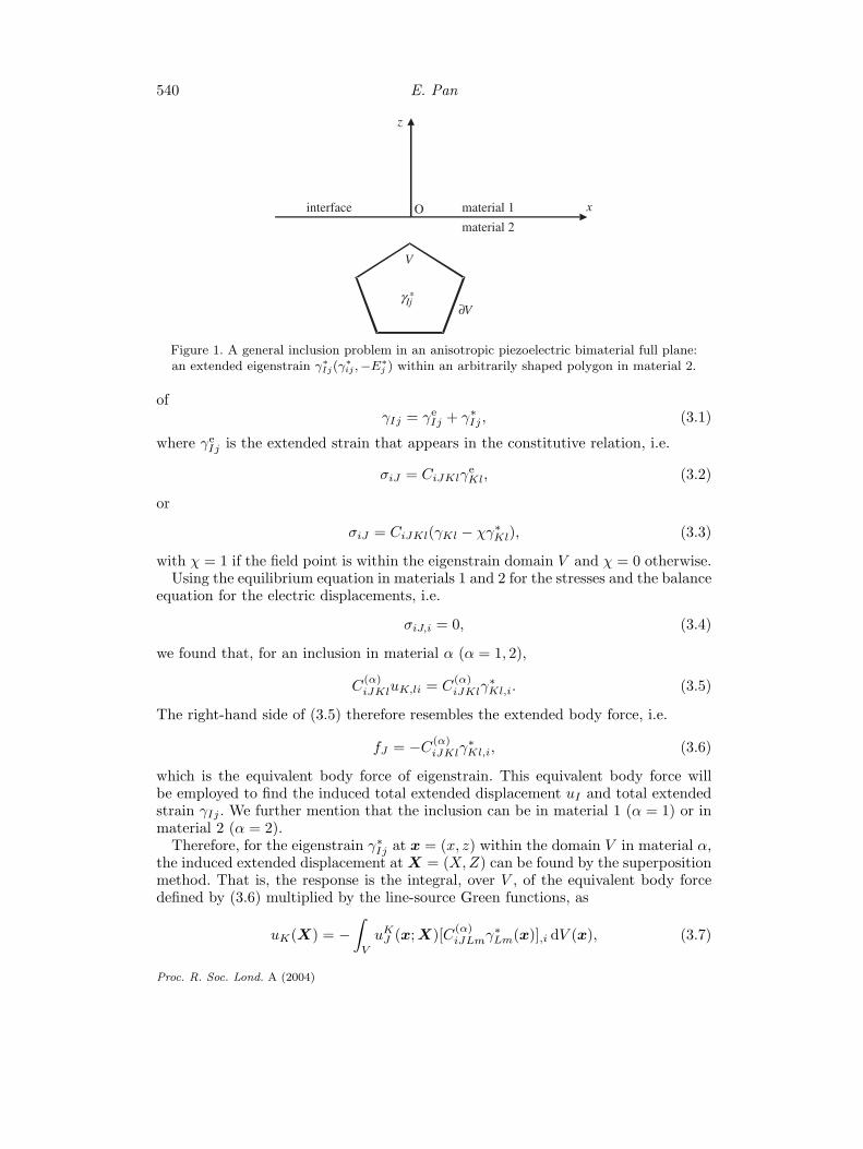
540 E. Pan
x
z
interface
*Ijγ
V
V
material 1
material 2O
∂
Figure 1. A general inclusion problem in an anisotropic piezoelectric bimaterial full plane:an extended eigenstrain γ∗
Ij(γ∗ij , −E∗
j ) within an arbitrarily shaped polygon in material 2.
ofγIj = γe
Ij + γ∗Ij , (3.1)
where γeIj is the extended strain that appears in the constitutive relation, i.e.
σiJ = CiJKlγeKl, (3.2)
or
σiJ = CiJKl(γKl − χγ∗Kl), (3.3)
with χ = 1 if the field point is within the eigenstrain domain V and χ = 0 otherwise.Using the equilibrium equation in materials 1 and 2 for the stresses and the balance
equation for the electric displacements, i.e.
σiJ,i = 0, (3.4)
we found that, for an inclusion in material α (α = 1, 2),
C(α)iJKluK,li = C
(α)iJKlγ
∗Kl,i. (3.5)
The right-hand side of (3.5) therefore resembles the extended body force, i.e.
fJ = −C(α)iJKlγ
∗Kl,i, (3.6)
which is the equivalent body force of eigenstrain. This equivalent body force willbe employed to find the induced total extended displacement uI and total extendedstrain γIj . We further mention that the inclusion can be in material 1 (α = 1) or inmaterial 2 (α = 2).
Therefore, for the eigenstrain γ∗Ij at x = (x, z) within the domain V in material α,
the induced extended displacement at X = (X, Z) can be found by the superpositionmethod. That is, the response is the integral, over V , of the equivalent body forcedefined by (3.6) multiplied by the line-source Green functions, as
uK(X) = −∫
V
uKJ (x; X)[C(α)
iJLmγ∗Lm(x)],i dV (x), (3.7)
Proc. R. Soc. Lond. A (2004)
Eshelby problem of polygonal inclusions 541
where uKJ (x; X) is the Green Jth elastic displacement/electric potential at x due to
a point-force/point-charge in the Kth direction applied at X. Depending upon thelocations of x and X, this Green function has four different sets of expressions andis derived in Appendix B.
Integrating by parts and noticing that the eigenstrain is non-zero only in V , equa-tion (3.7) can be expressed alternatively as
uK(X) =∫
V
uKJ,xi
(x; X)C(α)iJLmγ∗
Lm(x) dV (x). (3.8)
If we further assume that the eigenstrain is uniform within the domain V , then thedomain integral can be further transformed to the surface of V . That is
uK(X) = C(α)iJLmγ∗
Lm
∫∂V
uKJ (x; X)ni(x) dS(x), (3.9)
where ni(x) is the outward normal on the surface of V . Again, we mention that theinclusion can be in material 1 (α = 1) or material 2 (α = 2).
To find the elastic strain and electric fields, we take the derivatives of equation (3.9)with respect to the field point X (i.e. the source point of the line-force/line-chargeGreen function), which yields (for inclusion in material α),
γkp(X) = 12γ∗
LmC(α)iJLm
∫∂V
[ukJ,Xp
(x; X) + upJ,Xk
(x; X)]ni(x) dS(x),
k, p = 1, 2, 3, (3.10 a)
Ep(X) = −γ∗LmC
(α)iJLm
∫∂V
u4J,Xp
(x; X)ni(x) dS(x), p = 1, 2, 3. (3.10 b)
The stresses and electric displacements are obtained from (3.3) using material prop-erties in the corresponding domain.
We remark that the results presented are for the 2D-inclusion problem. Similarexpressions can be derived for the corresponding 3D problem. We also note that theinduced elastic and piezoelectric fields within the anisotropic piezoelectric bimateri-als can be obtained simply by performing an integral over the surface of the inclusion,provided that the corresponding bimaterial Green functions are available. Further-more, we will show next that, for a uniform piezoelectric eigenstrain field within anarbitrary polygon in a bimaterial full plane, the induced elastic and piezoelectricfields can be derived in the exact closed form. Such an exact closed-form solution isunavailable to the best of the author’s knowledge, except for the work by Faux etal . (1997), where they derived the eigenstrain-induced elastic field in a purely elasticisotropic full plane analytically using a similar approach to that presented in thispaper. With the bimaterial Green functions being derived in Appendix B for variousinterface conditions, we derive, in § 4, the exact closed-form solution for the inducedfield.
4. Analytical integral of an arbitrary line segment
First, we note that, in order to find the induced field due to a polygonal inclusion, oneneeds only to find the contribution from each straight-line segment of the bound-ary of the inclusion. The total induced field can be obtained by summing up thecontributions from all the sides of the polygon.
Proc. R. Soc. Lond. A (2004)
542 E. Pan
Now, to carry out the line integral in equation (3.9), we first write the extendedGreen displacement given by equations (B 1), (B 2), (B 16) and (B 17) in Appendix Bin the matrix form in the same way as we did for that in equation (3.9).
Therefore, when the source point is in material 1 (Z > 0), we have
uKJ (x, X) =
1π
Im{A(1)JR ln(z(1)
R − s(1)R )A(1)
KR} +1π
Im4∑
v=1
{A(1)JR ln(z(1)
R − s(1)v )Q11,v
RK }
(4.1 a)
for the field point in material 1 (z > 0), and
uKJ (x, X) =
1π
Im4∑
v=1
{A(2)JR ln(z(2)
R − s(1)v )Q12,v
RK } (4.1 b)
for the field point in material 2 (z < 0). In equations (4.1 a) and (4.2 b), an overbardenotes the complex conjugate, and superscripts (1) and (2) denote quantities inthe material half-planes 1 and 2, respectively. Definitions for z
(α)R and s
(α)v , and the
expressions for Q11,vRN and Q12,v
RN , are given in Appendix B.Similarly, when the source point is in material 2 (Z < 0), we have
uKJ (x, X) =
1π
Im4∑
v=1
{A(1)JR ln(z(1)
R − s(2)v )Q21,v
RK } (4.2 a)
for field point in material 1 (z > 0), and
uKJ (x, X) =
1π
Im{A(2)JR ln(z(2)
R − s(2)R )A(2)
KR} +1π
Im4∑
v=1
{A(2)JR ln(z(2)
R − s(2)v )Q22,v
RK }
(4.2 b)
for field point in material 2 (z < 0). Again, Q21,vRN and Q22,v
RN are given in Appendix B.Let us define a line segment in the (x, z)-plane starting from point 1 (x1, z1) and
ending at point 2 (x2, z2), in terms of the parameter t (0 � t � 1), as
x = x1 + (x2 − x1)t,
z = z1 + (z2 − z1)t.
}(4.3)
Therefore, the outward normal components ni(x) are constants, given by
n1 =(z2 − z1)
l, n2 = −(x2 − x1)
l, (4.4)
where l =√
(x2 − x1)2 + (z2 − z1)2 is the length of the line segment. It is obviousthat the elemental length is dS = l dt.
Note from Appendix B that, when the source and field points are in the samehalf-plane, the bimaterial Green functions consist of two parts: the full-plane Greenfunction and a complementary part. However, when they are in different half-planes,the bimaterial Green functions consist only a complementary part. Consequently, thecorresponding integrals can also be separated into two parts involving two types of
Proc. R. Soc. Lond. A (2004)
Eshelby problem of polygonal inclusions 543
functions. For the integral in the full plane, i.e. the first terms in (4.1 a) and (4.2 b),we define the result, being a function of the source point X ≡ (X, Z), as
h(α)R (X, Z) ≡
∫ 1
0ln(z(α)
R − s(α)R ) dt. (4.5)
Similarly, we define the integral corresponding to the complementary part as
gαβRv(X, Z) ≡
∫ 1
0ln(z(α)
R − s(β)v ) dt, (4.6 a)
w(α)Rv (X, Z) ≡
∫ 1
0ln(z(α)
R − s(α)v ) dt. (4.6 b)
While (4.6 a) corresponds to the line integration of (4.1 b) and (4.2 a), expres-sion (4.6 b) corresponds to the line integration of the second term in (4.1 a) and(4.2 b). The exact closed-form expressions for these integrals in (4.5) and (4.6) aregiven in Appendix C. Therefore, the induced elastic displacement and piezoelec-tric potential, due to the contribution of a straight line along the boundary, can beexpressed in an exact closed form. These are given below in detail.
When the inclusion is in material 1, the induced extended displacement is
uK(X) = niC(1)iJLmγ∗
Lm
l
πIm
{A
(1)JRh
(1)R (X, Z)A(1)
KR +4∑
v=1
A(1)JRw
(1)Rv(X, Z)Q11,v
RK
}(4.7 a)
for the response in material 1 (Z > 0), and
uK(X) = niC(1)iJLmγ∗
Lm
l
πIm
{ 4∑v=1
A(1)JRg12
Rv(X, Z)Q21,vRK
}(4.7 b)
for the response in material 2 (Z < 0).Similarly, when the inclusion is in material 2, the induced extended displacement is
uK(X) = niC(2)iJLmγ∗
Lm
l
πIm
{ 4∑v=1
A(2)JRg21
Rv(X, Z)Q12,vRK
}(4.7 c)
for the response in material 1 (Z > 0) and
uK(X) = niC(2)iJLmγ∗
Lm
l
πIm
{A
(2)JRh
(2)R (X, Z)A(2)
KR +4∑
v=1
A(2)JRw
(2)Rv(X, Z)Q22,v
RK
}(4.7 d)
for the response in material 2 (Z < 0).Note that the first term is the solution corresponding to the full plane, and the
second term is the contribution from the complementary part, which is used tosatisfy the interface conditions of the bimaterials. Therefore, equations (4.7) give thecontribution of a straight-line segment of the inclusion in the bimaterials with theinclusion being in either of the half-planes. By adding contributions from all the linesegments of the boundary of the inclusion, the extended displacement solution foran inclusion with a general polygonal shape in either half-plane is then obtained inan exact closed form!
Proc. R. Soc. Lond. A (2004)
544 E. Pan
The exact closed-form strain and electric field can be obtained by simply takingthe derivatives of (4.7 a)–(4.7 d) with respect to the coordinate X = (X, Z). In doingso, we obtain the elastic strain and electric field, due to a straight-line segment ofthe boundary of the inclusion, by the following equations (for α, β = 1, 3).
When the inclusion is in material 1, we have
γβα(X)
= 0.5niC(1)iJLmγ∗
Lm
l
πIm
{A
(1)JRh
(1)R,α(X, Z)A(1)
βR +4∑
v=1
A(1)JRw
(1)Rv,α(X, Z)Q11,v
Rβ
}
+ 0.5niC(1)iJLmγ∗
Lm
l
πIm
{A
(1)JRh
(1)R,β(X, Z)A(1)
αR +4∑
v=1
A(1)JRw
(1)Rv,β(X, Z)Q11,v
Rα
},
γ2α(X)
= 0.5niC(1)iJLmγ∗
Lm
l
πIm
{A
(1)JRh
(1)R,α(X, Z)A(1)
2R +4∑
v=1
A(1)JRw
(1)Rv,α(X, Z)Q11,v
R2
},
Eα(X)
= −niC(1)iJLmγ∗
Lm
l
πIm
{A
(1)JRh
(1)R,α(X, Z)A(1)
4R +4∑
v=1
A(1)JRw
(1)Rv,α(X, Z)Q11,v
R4
}
(4.8)for the response in material 1 (Z > 0), and
γβα(X)
= 0.5niC(1)iJLmγ∗
Lm
l
πIm
{ 4∑v=1
A(1)JRg12
Rv,α(X, Z)Q21,vRβ +
4∑v=1
A(1)JRg12
Rv,β(X, Z)Q21,vRα
},
(4.9)
γ2α(X) = 0.5niC(1)iJLmγ∗
Lm
l
πIm
{ 4∑v=1
A(1)JRg12
Rv,α(X, Z)Q21,vR2
}, (4.10)
Eα(X) = −niC(1)iJLmγ∗
Lm
l
πIm
{ 4∑v=1
A(1)JRg12
Rv,α(X, Z)Q21,vR4
}, (4.11)
for the response in material 2 (Z < 0).Similarly, when the inclusion is in material 2, we obtain
γβα(X)
= 0.5niC(2)iJLmγ∗
Lm
l
πIm
{ 4∑v=1
A(2)JRg21
Rv,α(X, Z)Q12,vRβ +
4∑v=1
A(2)JRg21
Rv,β(X, Z)Q12,vRα
},
(4.12)
γ2α(X) = 0.5niC(2)iJLmγ∗
Lm
l
πIm
{ 4∑v=1
A(2)JRg21
Rv,α(X, Z)Q12,vR2
}, (4.13)
Eα(X) = −niC(2)iJLmγ∗
Lm
l
πIm
{ 4∑v=1
A(2)JRg21
Rv,α(X, Z)Q12,vR4
}, (4.14)
Proc. R. Soc. Lond. A (2004)
Eshelby problem of polygonal inclusions 545
for the response in material 1 (Z > 0), and
γβα(X)
= 0.5niC(2)iJLmγ∗
Lm
l
πIm
{A
(2)JRh
(2)R,α(X, Z)A(2)
βR +4∑
v=1
A(2)JRw
(2)Rv,α(X, Z)Q22,v
Rβ
}
+ 0.5niC(2)iJLmγ∗
Lm
l
πIm
{A
(2)JRh
(2)R,β(X, Z)A(2)
αR +4∑
v=1
A(2)JRw
(2)Rv,β(X, Z)Q22,v
Rα
},
γ2α(X)
= 0.5niC(2)iJLmγ∗
Lm
l
πIm
{A
(2)JRh
(2)R,α(X, Z)A(2)
2R +4∑
v=1
A(2)JRw
(2)Rv,α(X, Z)Q22,v
R2
},
Eα(X)
= −niC(2)iJLmγ∗
Lm
l
πIm
{A
(2)JRh
(2)R,α(X, Z)A(2)
4R +4∑
v=1
A(2)JRw
(2)Rv,α(X, Z)Q22,v
R4
}
(4.15)for the response in material 2 (Z < 0). In equations (4.8)–(4.15), the involved func-tions of (X, Z) are given in Appendix C.
As a generalization, equations (4.8)–(4.15) can be written as
γIj = SIjLmγ∗Lm, (4.16)
where SIjLm is the total Eshelby tensor in the bimaterial full plane. On observationof the induced strain/electric fields (equations (4.8)–(4.15)), the total Eshelby tensorcan be expressed as
SIjLm = S∞IjLm + Sc
IjLm, (4.17)
where the first term is the Eshelby tensor in an anisotropic piezoelectric homogeneousfull plane, and the second term is the one corresponding to the complementarycontribution due to the material mismatch of the bimaterials.
With these strain and electric field solutions, the stresses and electric displacementsare then found from equation (3.3), using the material properties corresponding tothe suitable half-plane. In summary, therefore, we have derived the exact closed-form solutions for the elastic and piezoelectric fields induced by an inclusion withinan arbitrary polygon in a bimaterial full plane. Since our solutions are in the exactclosed form, multiple-inclusion problems can be solved simply by superposing thecontributions from all the inclusions. Furthermore, a solution to the inclusion witha curved boundary can also be obtained by approximating the curvilinear elementwith a straight-line element.
5. Numerical examples
First, the formulation has been checked for a couple of examples. For instance, whenmaterials 1 and 2 are identical, the inclusion solution will then reduce to the full-planesolution (Pan 2004); when one of the two material half-planes has material properties10 orders smaller than the other, our bimaterial-inclusion solution reduces to thehalf-plane solution (Pan 2004). We further mention that various inclusion solutionsin isotropic elasticity have been also checked carefully, including a polygonal inclusionin full- and half-planes (Rodin 1996; Faux et al . 1997; Glas 2002).
Proc. R. Soc. Lond. A (2004)
546 E. Pan
Having checked our bimaterial inclusion solutions, we now apply our solution toan inclusion in a real bimaterial full plane. The bimaterials are made of two typicalpiezoelectric materials (Pan 2002c): one is a left-hand quartz in a rotated coordinatesystem (Tiersten 1969) with elastic constants, piezoelectric coefficients and dielectricconstants being, respectively,
[C
]=
0.8674 −0.0825 0.2715 −0.0366 0 0−0.0825 1.2977 −0.0742 0.057 0 00.2715 −0.0742 1.0283 0.0992 0 0
−0.0366 0.057 0.0992 0.3861 0 00 0 0 0 0.6881 0.02530 0 0 0 0.0253 0.2901
(1011 N m−2),
(5.1 a)
[e]
=
0.171 −0.152 −0.0187 0.067 0 0
0 0 0 0 0.108 −0.0950 0 0 0 −0.0761 0.067
(C m−2), (5.1 b)
[ε]
=
0.3921 0 0
0 0.3982 0.00860 0.0086 0.4042
(10−10 C V−1 m−1). (5.1 c)
The other one is the poled lead-zirconate-titanate (PZT-4) ceramic (Dunn & Taya1993) with elastic constants, piezoelectric coefficients and dielectric constants being,respectively,
[C
]=
1.39 0.778 0.743 0 0 00.778 1.39 0.743 0 0 00.743 0.743 1.15 0 0 0
0 0 0 0.256 0 00 0 0 0 0.256 00 0 0 0 0 0.306
(1011 N m−2), (5.2 a)
[e]
=
0 0 0 0 12.7 0
0 0 0 12.7 0 0−5.2 −5.2 15.1 0 0 0
(C m−2), (5.2 b)
[ε]
=
0.646 05 0 0
0 0.646 05 00 0 0.561 975
(10−8 C V m). (5.2 c)
We remark that, while the quartz is a weakly coupled piezoelectric material, theceramic is a strongly coupled one, with the degree of the electromechanical coupling,defined as
g =emax√
(εmaxCmax),
being equal to 0.07 and 0.5 in quartz and ceramic, respectively.Two bimaterial cases are considered. For case 1, named quartz/ceramic, material 1
(i.e. the upper half-plane with z > 0) is quartz and material 2 (i.e. the lower half-plane with z < 0) is ceramic. For case 2, named ceramic/quartz, material 1 is ceramic
Proc. R. Soc. Lond. A (2004)
Eshelby problem of polygonal inclusions 547
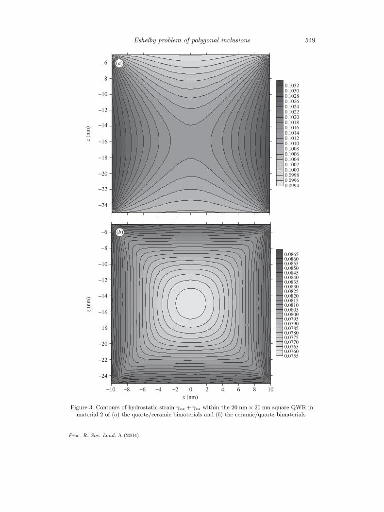
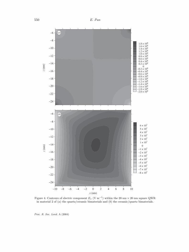
and material 2 is quartz. For both cases, there is a 20 nm × 20 nm square QWRin material 2, and it is symmetrically located with respect to the z-axis, with itsupper side 5 nm from the interface. The eigenstrain in the inclusion is assumed to behydrostatic with γ∗
xx = γ∗zz = 0.07, a typical magnitude in the InAs/GaAs quantum
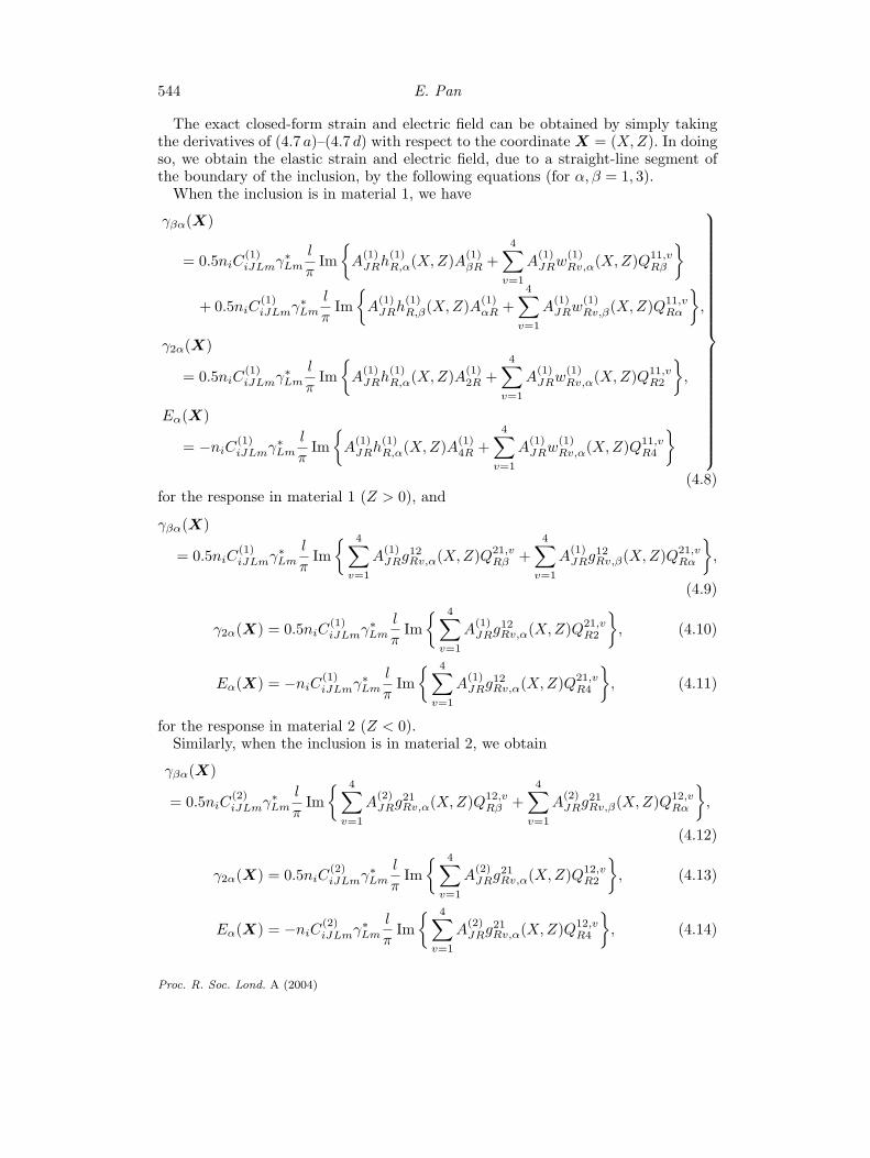
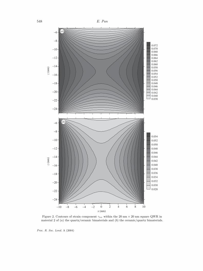
structure (Bimberg et al . 1999).Figure 2a shows the contours of strain component γxx within the square QWR in
material 2 of the quartz/ceramic, while figure 2b shows the same strain componentfor the ceramic/quartz. Note that, while the contours show certain similarities, theirmagnitudes are different. In particular, the magnitude of this strain component isslightly larger than the given eigenstrain (0.072 versus 0.07) when the bimaterial fullplane is quartz/ceramic (figure 2a), and smaller than the given eigenstrain (0.054versus 0.07) when it is ceramic/quartz (figure 2b).
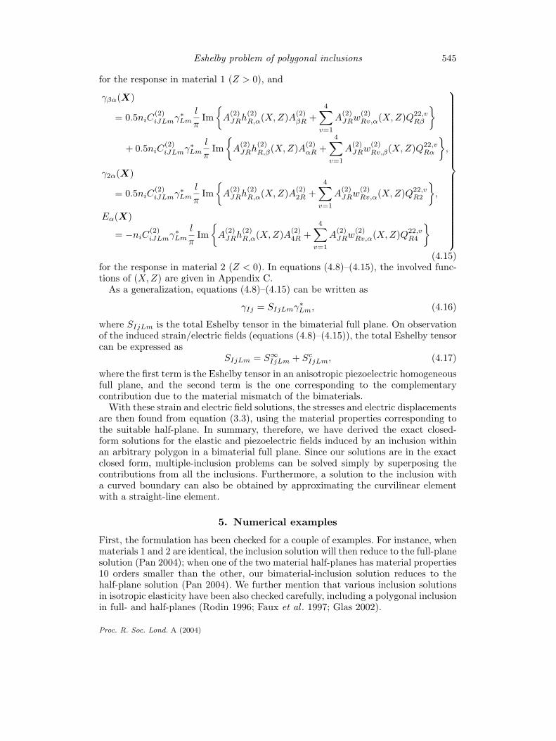
Similarly, figure 3a, b shows the contours of hydrostatic strain γxx +γzz within thesquare QWR in material 2 of quartz/ceramic and of ceramic/quartz, respectively. Itis interesting that, for both bimaterial cases, the induced hydrostatic strain withinthe square QWR is roughly constant, with a value of 0.1 for the quartz/ceramic(figure 3a) and 0.085 for the ceramic/quartz (figure 3b). We remark that the samenear-constant feature for the hydrostatic strain was also observed for a rectangularinclusion in an isotropic full plane (Downes et al . 1995).
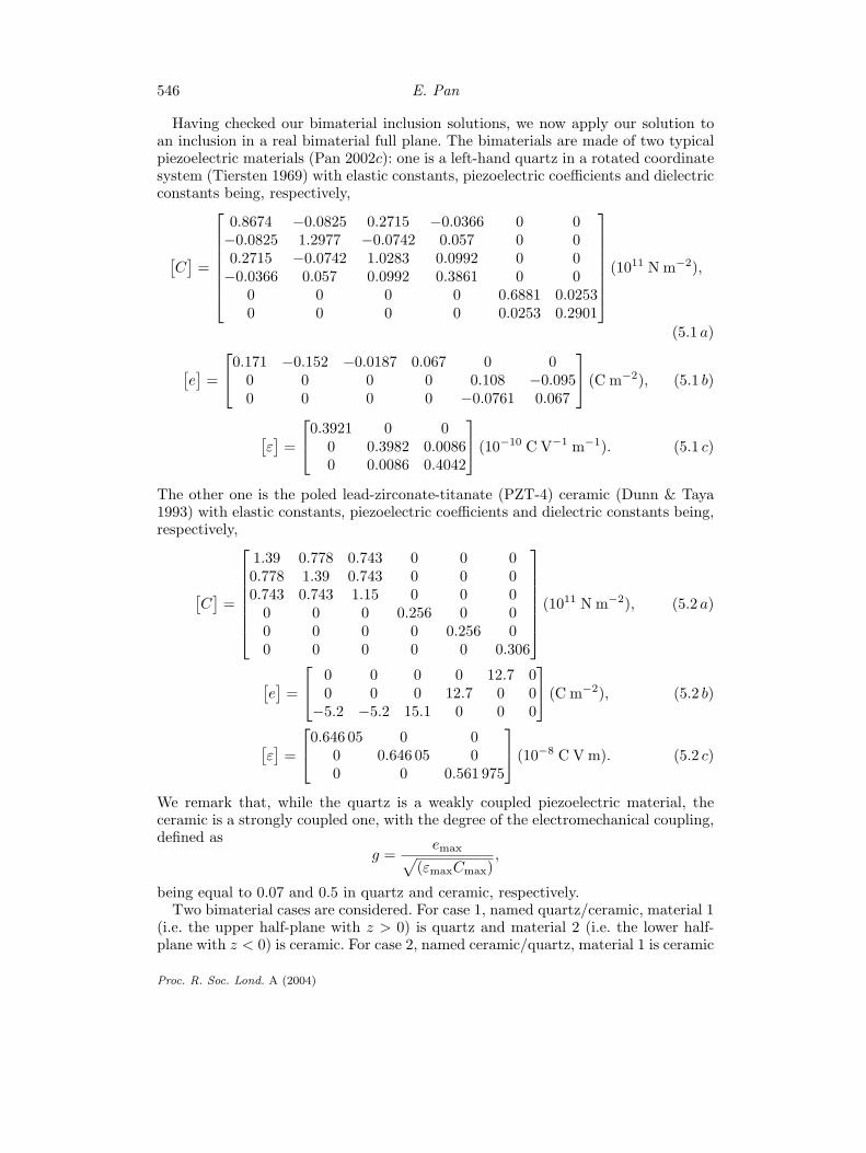
The contour of electric component Ex (V m−1) within the square QWR in mate-rial 2 of the quartz/ceramic is plotted in figure 4a. The corresponding result is shownin figure 4b for the ceramic/quartz case. We note that the induced Ex is completelydifferent for the two bimaterial systems. Their contour shapes and magnitudes areclearly different from each other for the two bimaterial cases. In particular, the max-imum magnitude in quartz/ceramic is roughly twice that in ceramic/quartz. Also,we observe that the distribution of the electric component Ex for the ceramic/quartzcase (figure 4b) is asymmetric, due to the fact that the quartz has been rotated tobecome a low-symmetry monoclinic material (see equations (5.1)).
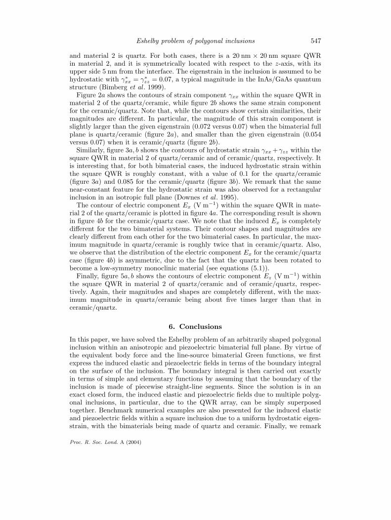
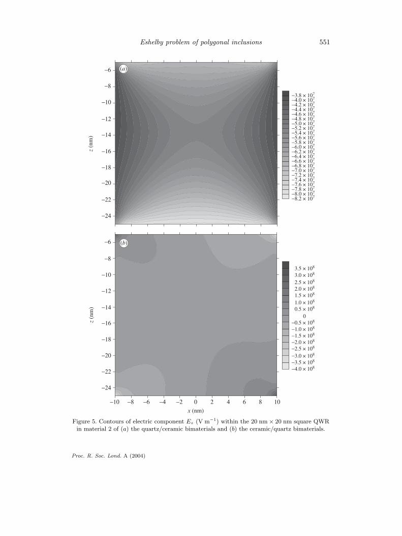
Finally, figure 5a, b shows the contours of electric component Ez (V m−1) withinthe square QWR in material 2 of quartz/ceramic and of ceramic/quartz, respec-tively. Again, their magnitudes and shapes are completely different, with the max-imum magnitude in quartz/ceramic being about five times larger than that inceramic/quartz.
6. Conclusions
In this paper, we have solved the Eshelby problem of an arbitrarily shaped polygonalinclusion within an anisotropic and piezoelectric bimaterial full plane. By virtue ofthe equivalent body force and the line-source bimaterial Green functions, we firstexpress the induced elastic and piezoelectric fields in terms of the boundary integralon the surface of the inclusion. The boundary integral is then carried out exactlyin terms of simple and elementary functions by assuming that the boundary of theinclusion is made of piecewise straight-line segments. Since the solution is in anexact closed form, the induced elastic and piezoelectric fields due to multiple polyg-onal inclusions, in particular, due to the QWR array, can be simply superposedtogether. Benchmark numerical examples are also presented for the induced elasticand piezoelectric fields within a square inclusion due to a uniform hydrostatic eigen-strain, with the bimaterials being made of quartz and ceramic. Finally, we remark
Proc. R. Soc. Lond. A (2004)
548 E. Pan
−24
−22
−20
−18
−16
−14
−12
−10
−8
−6
0.0380.0400.0420.0440.0460.0480.0500.0520.0540.0560.0580.0600.0620.0640.0660.0680.0700.072
−10 −8 −6 −4 −2 0 10
0.028
0.030
0.032
0.034
0.036
0.038
0.040
0.042
0.044
0.046
0.048
0.050
0.052
0.054
z (n
m)
−24
−22
−20
−18
−16
−14
−12
−10
−8
−6
z (n
m)
2 4 6 8
x (nm)
(a)
(b)
Figure 2. Contours of strain component γxx within the 20 nm × 20 nm square QWR inmaterial 2 of (a) the quartz/ceramic bimaterials and (b) the ceramic/quartz bimaterials.
Proc. R. Soc. Lond. A (2004)
Eshelby problem of polygonal inclusions 549
−10
−24
−22
−20
−18
−16
−14
−12
−10
−8
−6
z (n
m)
−24
−22
−20
−18
−16
−14
−12
−10
−8
−6
z (n
m)
0.09940.09960.09980.10000.10020.10040.10060.10080.10100.10120.10140.10160.10180.10200.10220.10240.10260.10280.10300.1032
−8 −6 −4 −2 0 102 4 6 8x (nm)
0.07550.07600.07650.07700.07750.07800.07850.07900.07950.08000.08050.08100.08150.08200.08250.08300.08350.08400.08450.08500.08550.08600.0865
(b)
(a)
Figure 3. Contours of hydrostatic strain γxx + γzz within the 20 nm × 20 nm square QWR inmaterial 2 of (a) the quartz/ceramic bimaterials and (b) the ceramic/quartz bimaterials.
Proc. R. Soc. Lond. A (2004)
550 E. Pan
−10
−24
−22
−20
−18
−16
−14
−12
−10
−8
−6
z (n
m)
−24
−22
−20
−18
−16
−14
−12
−10
−8
−6
z (n
m)
−8 −6 −4 −2 0 102 4 6 8x (nm)
−2.0 × 10⁸−1.8 × 10⁸−1.6 × 10⁸−1.4 × 10⁸−1.2 × 10⁸−1.0 × 10⁸−0.8 × 10⁸−0.6 × 10⁸−0.4 × 10⁸−0.2 × 10⁸
00.2 × 1080.4 × 1080.6 × 1080.8 × 1081.0 × 1081.2 × 1081.4 × 1081.6 × 1081.8 × 108
−8 × 10⁷−7 × 10⁷−6 × 10⁷−5 × 10⁷−4 × 10⁷−3 × 10⁷−2 × 10⁷−1 × 10⁷
01 × 1072 × 1073 × 1074 × 1075 × 1076 × 107
(a)
(b)
Figure 4. Contours of electric component Ex (V m−1) within the 20 nm × 20 nm square QWRin material 2 of (a) the quartz/ceramic bimaterials and (b) the ceramic/quartz bimaterials.
Proc. R. Soc. Lond. A (2004)
Eshelby problem of polygonal inclusions 551
−10
−24
−22
−20
−18
−16
−14
−12
−10
−8
−6
z (n
m)
−24
−22
−20
−18
−16
−14
−12
−10
−8
−6
z (n
m)
−8 −6 −4 −2 0 102 4 6 8x (nm)
−4.0 × 10⁸−3.5 × 10⁸−3.0 × 10⁸−2.5 × 10⁸−2.0 × 10⁸−1.5 × 10⁸−1.0 × 10⁸−0.5 × 10⁸
00.5 × 1081.0 × 1081.5 × 1082.0 × 1082.5 × 1083.0 × 108
−8.2 × 10⁷−8.0 × 10⁷−7.8 × 10⁷−7.6 × 10⁷−7.4 × 10⁷−7.2 × 10⁷−7.0 × 10⁷−6.8 × 10⁷−6.6 × 10⁷−6.4 × 10⁷−6.2 × 10⁷−6.0 × 10⁷−5.8 × 10⁷−5.6 × 10⁷−5.4 × 10⁷−5.2 × 10⁷−5.0 × 10⁷−4.8 × 10⁷−4.6 × 10⁷−4.4 × 10⁷−4.2 × 10⁷−4.0 × 10⁷−3.8 × 10⁷
3.5 × 10⁸
(b)
(a)
Figure 5. Contours of electric component Ez (V m−1) within the 20 nm × 20 nm square QWRin material 2 of (a) the quartz/ceramic bimaterials and (b) the ceramic/quartz bimaterials.
Proc. R. Soc. Lond. A (2004)
552 E. Pan
that the present exact closed-form solution includes the solution to the correspondinganisotropic elastic bimaterials as its special case and, furthermore, contains a totalof six different interface models which may be useful in the piezoelectric bimaterialanalysis and design.
The author thanks both reviewers for their constructive comments, and the University of Akronfor partial support under Grant no. 2-07522.
Appendix A. Five imperfect interface models andthe corresponding modified matrices
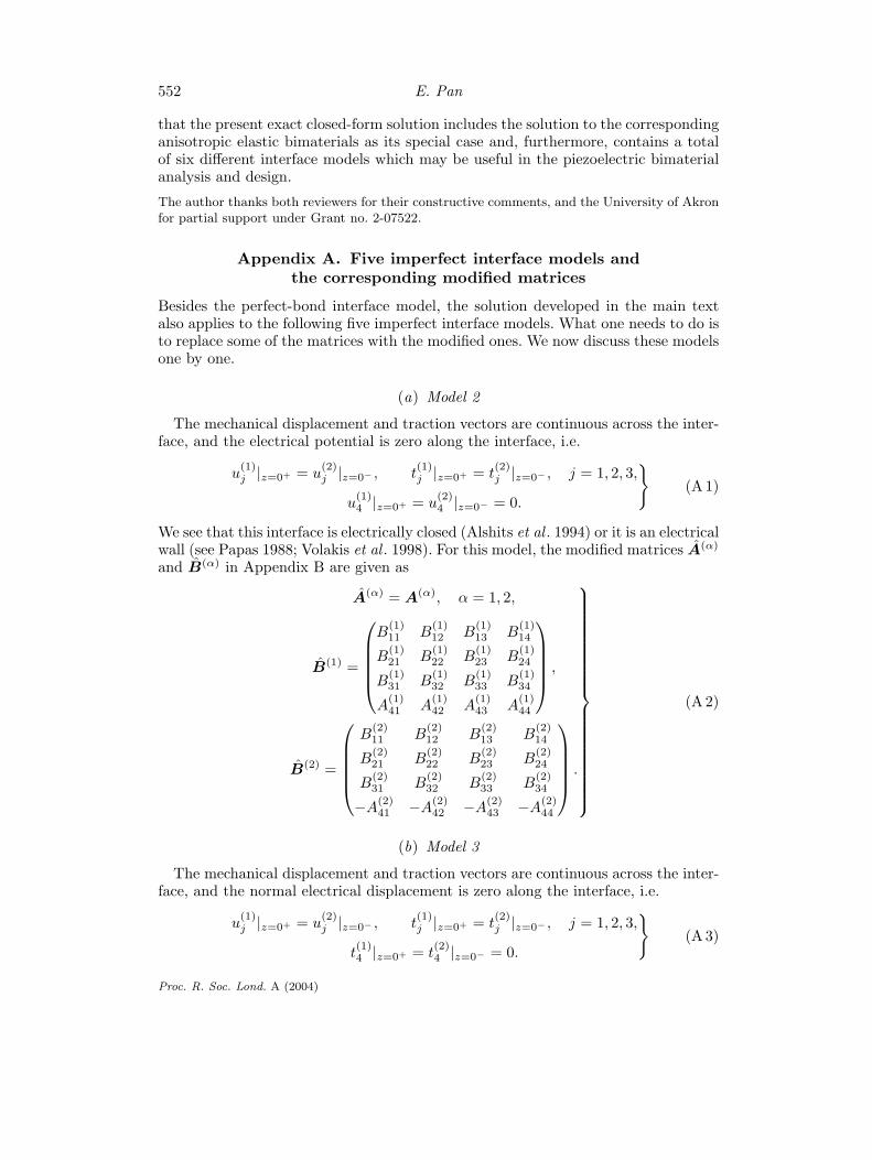
Besides the perfect-bond interface model, the solution developed in the main textalso applies to the following five imperfect interface models. What one needs to do isto replace some of the matrices with the modified ones. We now discuss these modelsone by one.
(a) Model 2
The mechanical displacement and traction vectors are continuous across the inter-face, and the electrical potential is zero along the interface, i.e.
u(1)j |z=0+ = u
(2)j |z=0− , t
(1)j |z=0+ = t
(2)j |z=0− , j = 1, 2, 3,
u(1)4 |z=0+ = u
(2)4 |z=0− = 0.
}(A 1)
We see that this interface is electrically closed (Alshits et al . 1994) or it is an electricalwall (see Papas 1988; Volakis et al . 1998). For this model, the modified matrices A(α)
and B(α) in Appendix B are given as
A(α) = A(α), α = 1, 2,
B(1) =
B(1)11 B
(1)12 B
(1)13 B
(1)14
B(1)21 B
(1)22 B
(1)23 B
(1)24
B(1)31 B
(1)32 B
(1)33 B
(1)34
A(1)41 A
(1)42 A
(1)43 A
(1)44
,
B(2) =
B(2)11 B
(2)12 B
(2)13 B
(2)14
B(2)21 B
(2)22 B
(2)23 B
(2)24
B(2)31 B
(2)32 B
(2)33 B
(2)34
−A(2)41 −A
(2)42 −A
(2)43 −A
(2)44
.
(A 2)
(b) Model 3
The mechanical displacement and traction vectors are continuous across the inter-face, and the normal electrical displacement is zero along the interface, i.e.
u(1)j |z=0+ = u
(2)j |z=0− , t
(1)j |z=0+ = t
(2)j |z=0− , j = 1, 2, 3,
t(1)4 |z=0+ = t
(2)4 |z=0− = 0.
}(A 3)
Proc. R. Soc. Lond. A (2004)
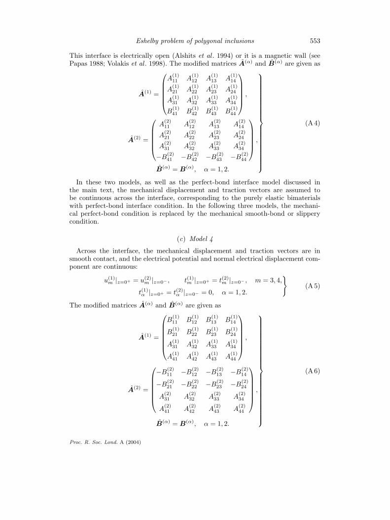
Eshelby problem of polygonal inclusions 553
This interface is electrically open (Alshits et al . 1994) or it is a magnetic wall (seePapas 1988; Volakis et al . 1998). The modified matrices A(α) and B(α) are given as
A(1) =
A(1)11 A
(1)12 A
(1)13 A
(1)14
A(1)21 A
(1)22 A
(1)23 A
(1)24
A(1)31 A
(1)32 A
(1)33 A
(1)34
B(1)41 B
(1)42 B
(1)43 B
(1)44
,
A(2) =
A(2)11 A
(2)12 A
(2)13 A
(2)14
A(2)21 A
(2)22 A
(2)23 A
(2)24
A(2)31 A
(2)32 A
(2)33 A
(2)34
−B(2)41 −B
(2)42 −B
(2)43 −B
(2)44
,
B(α) = B(α), α = 1, 2.
(A 4)
In these two models, as well as the perfect-bond interface model discussed inthe main text, the mechanical displacement and traction vectors are assumed tobe continuous across the interface, corresponding to the purely elastic bimaterialswith perfect-bond interface condition. In the following three models, the mechani-cal perfect-bond condition is replaced by the mechanical smooth-bond or slipperycondition.
(c) Model 4
Across the interface, the mechanical displacement and traction vectors are insmooth contact, and the electrical potential and normal electrical displacement com-ponent are continuous:
u(1)m |z=0+ = u(2)
m |z=0− , t(1)m |z=0+ = t(2)m |z=0− , m = 3, 4,
t(1)α |z=0+ = t(2)α |z=0− = 0, α = 1, 2.
}(A 5)
The modified matrices A(α) and B(α) are given as
A(1) =
B(1)11 B
(1)12 B
(1)13 B
(1)14
B(1)21 B
(1)22 B
(1)23 B
(1)24
A(1)31 A
(1)32 A
(1)33 A
(1)34
A(1)41 A
(1)42 A
(1)43 A
(1)44
,
A(2) =
−B(2)11 −B
(2)12 −B
(2)13 −B
(2)14
−B(2)21 −B
(2)22 −B
(2)23 −B
(2)24
A(2)31 A
(2)32 A
(2)33 A
(2)34
A(2)41 A
(2)42 A
(2)43 A
(2)44
,
B(α) = B(α), α = 1, 2.
(A 6)
Proc. R. Soc. Lond. A (2004)
554 E. Pan
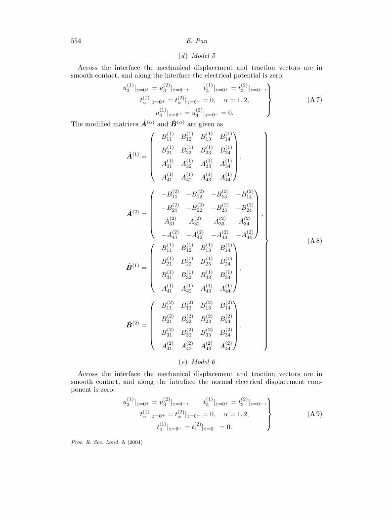
(d) Model 5
Across the interface the mechanical displacement and traction vectors are insmooth contact, and along the interface the electrical potential is zero:
u(1)3 |z=0+ = u
(2)3 |z=0− , t
(1)3 |z=0+ = t
(2)3 |z=0− ,
t(1)α |z=0+ = t(2)α |z=0− = 0, α = 1, 2,
u(1)4 |z=0+ = u
(2)4 |z=0− = 0.
(A 7)
The modified matrices A(α) and B(α) are given as
A(1) =
B(1)11 B
(1)12 B
(1)13 B
(1)14
B(1)21 B
(1)22 B
(1)23 B
(1)24
A(1)31 A
(1)32 A
(1)33 A
(1)34
A(1)41 A
(1)42 A
(1)43 A
(1)44
,
A(2) =
−B(2)11 −B
(2)12 −B
(2)13 −B
(2)14
−B(2)21 −B
(2)22 −B
(2)23 −B
(2)24
A(2)31 A
(2)32 A
(2)33 A
(2)34
−A(2)41 −A
(2)42 −A
(2)43 −A
(2)44
,
B(1) =
B(1)11 B
(1)12 B
(1)13 B
(1)14
B(1)21 B
(1)22 B
(1)23 B
(1)24
B(1)31 B
(1)32 B
(1)33 B
(1)34
A(1)41 A
(1)42 A
(1)43 A
(1)44
,
B(2) =
B(2)11 B
(2)12 B
(2)13 B
(2)14
B(2)21 B
(2)22 B
(2)23 B
(2)24
B(2)31 B
(2)32 B
(2)33 B
(2)34
A(2)41 A
(2)42 A
(2)43 A
(2)44
.
(A 8)
(e) Model 6
Across the interface the mechanical displacement and traction vectors are insmooth contact, and along the interface the normal electrical displacement com-ponent is zero:
u(1)3 |z=0+ = u
(2)3 |z=0− , t
(1)3 |z=0+ = t
(2)3 |z=0− ,
t(1)α |z=0+ = t(2)α |z=0− = 0, α = 1, 2,
t(1)4 |z=0+ = t
(2)4 |z=0− = 0.
(A 9)
Proc. R. Soc. Lond. A (2004)
Eshelby problem of polygonal inclusions 555
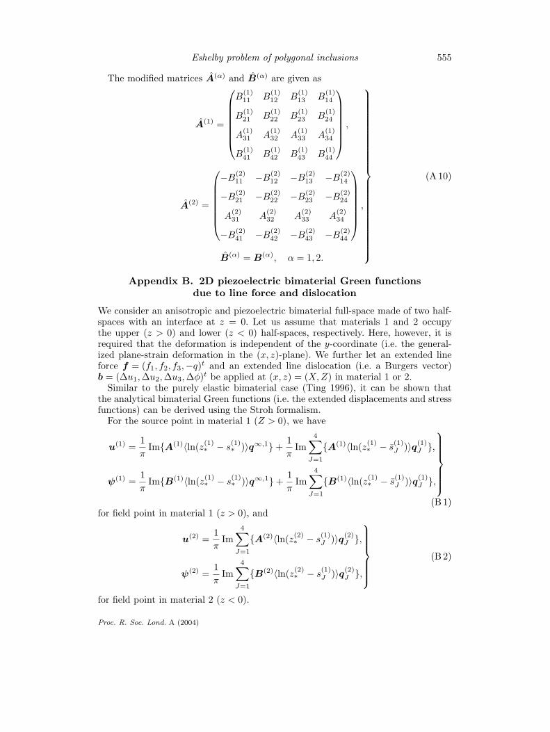
The modified matrices A(α) and B(α) are given as
A(1) =
B(1)11 B
(1)12 B
(1)13 B
(1)14
B(1)21 B
(1)22 B
(1)23 B
(1)24
A(1)31 A
(1)32 A
(1)33 A
(1)34
B(1)41 B
(1)42 B
(1)43 B
(1)44
,
A(2) =
−B(2)11 −B
(2)12 −B
(2)13 −B
(2)14
−B(2)21 −B
(2)22 −B
(2)23 −B
(2)24
A(2)31 A
(2)32 A
(2)33 A
(2)34
−B(2)41 −B
(2)42 −B
(2)43 −B
(2)44
,
B(α) = B(α), α = 1, 2.
(A 10)
Appendix B. 2D piezoelectric bimaterial Green functionsdue to line force and dislocation
We consider an anisotropic and piezoelectric bimaterial full-space made of two half-spaces with an interface at z = 0. Let us assume that materials 1 and 2 occupythe upper (z > 0) and lower (z < 0) half-spaces, respectively. Here, however, it isrequired that the deformation is independent of the y-coordinate (i.e. the general-ized plane-strain deformation in the (x, z)-plane). We further let an extended lineforce f = (f1, f2, f3, −q)t and an extended line dislocation (i.e. a Burgers vector)b = (∆u1, ∆u2, ∆u3, ∆φ)t be applied at (x, z) = (X, Z) in material 1 or 2.
Similar to the purely elastic bimaterial case (Ting 1996), it can be shown thatthe analytical bimaterial Green functions (i.e. the extended displacements and stressfunctions) can be derived using the Stroh formalism.
For the source point in material 1 (Z > 0), we have
u(1) =1π
Im{A(1)〈ln(z(1)∗ − s
(1)∗ )〉q∞,1} +
1π
Im4∑
J=1
{A(1)〈ln(z(1)∗ − s
(1)J )〉q(1)
J },
ψ(1) =1π
Im{B(1)〈ln(z(1)∗ − s
(1)∗ )〉q∞,1} +
1π
Im4∑
J=1
{B(1)〈ln(z(1)∗ − s
(1)J )〉q(1)
J },
(B 1)for field point in material 1 (z > 0), and
u(2) =1π
Im4∑
J=1
{A(2)〈ln(z(2)∗ − s
(1)J )〉q(2)
J },
ψ(2) =1π
Im4∑
J=1
{B(2)〈ln(z(2)∗ − s
(1)J )〉q(2)
J },
(B 2)
for field point in material 2 (z < 0).
Proc. R. Soc. Lond. A (2004)
556 E. Pan
In equations (B 1) and (B 2), ψ is the extended stress function vector related tothe elastic stresses and electrical displacements by
σ1J = −ψJ,3; σ3J = ψJ,1. (B 3)
Also in equations (B 1) and (B 2), ‘Im’ stands for the imaginary part, and the super-scripts ‘(1)’ and ‘(2)’ denote, as in the text, the quantities associated with the mate-rial domains 1 and 2, respectively; p
(α)J , A(α), and B(α) are the Stroh eigenvalues
and matrices. They are solutions of the eigenequation discussed in Appendix A ofPan (2004). Finally, in equations (B 1) and (B 2),
〈ln(z(1)∗ − s
(1)∗ )〉
= diag[ln(z(1)1 − s
(1)1 ), ln(z(1)
2 − s(1)2 ), ln(z(1)
3 − s(1)3 ), ln(z(1)
4 − s(1)4 )],
〈ln(z(α)∗ − s
(1)J )〉
= diag[ln(z(α)1 − s
(1)J ), ln(z(α)
2 − s(1)J ), ln(z(α)
3 − s(1)J ), ln(z(α)
4 − s(1)J )]
(α = 1, 2),
(B 4)with the complex variable z
(α)J and s
(α)J being defined by
z(α)J = x + p
(α)J z, (B 5)
s(α)J = X + p
(α)J Z. (B 6)
Note that the first term in equation (B 1) corresponds to the full-plane Green func-tions (with material properties of material 1) with
q∞,1 = (A(1))Tf + (B(1))Tb. (B 7)
The second term in equation (B 1) and the solution in material 2 (B 2) are thecomplementary parts of the solution with the complex constant vectors q
(α)J (α = 1, 2,
J = 1, 2, 3, 4) to be determined.For a perfect-bond interface at z = 0, it can be shown that the constant vectors
q(α)J satisfy the conditions (J = 1, 2, 3, 4)
A(1)q(1)J + A(2)q
(2)J = A(1)IJ q∞,1,
B(1)q(1)J + B(2)q
(2)J = B(1)IJ q∞,1,
}(B 8)
withI1 = diag[1, 0, 0, 0], I2 = diag[0, 1, 0, 0],
I3 = diag[0, 0, 1, 0], I4 = diag[0, 0, 0, 1].
}(B 9)
The solutions of the vectors are readily found to be
q(1)J = (A(1))−1(M (1) + M (2))−1(M (2) − M (1))A(1)IJ q∞,1,
q(2)J = (A(2))−1(M (1) + M (2))−1(M (1) + M (1))A(1)IJq∞,1,
}(B 10)
where M (α) are the impedance tensors, defined as
M (α) = −iB(α)(A(α))−1, α = 1, 2. (B 11)
Proc. R. Soc. Lond. A (2004)
Eshelby problem of polygonal inclusions 557
The complex constants involved in the bimaterial Green solutions (B 1) and (B 2)for the five interface models discussed in Appendix A can also be determined byfollowing the same procedure. As in equation (B 10), the solutions can be written as
q(1)J = (A(1))−1(M (1) + ¯
M (2))−1( ¯M (2) − ¯
M (1) ¯A(1)IJ q∞,1
≡ K11IJ q∞,1,
q(2)J = (A(2))−1( ¯
M (1) + M (2))−1(M (1) + ¯M (1))A(1)IJq∞,1
≡ K12IJq∞,1,
(B 12)
where M (α) (α = 1, 2) are the modified impedance tensors defined as
M (α) = −iB(α)(A(α))−1, α = 1, 2, (B 13)
and the modified matrices A(α) and B(α) (α = 1, 2) are given in Appendix A forthe five imperfect interface models. Equation (B 12) is for the five imperfect inter-face models as well as for the perfect-bond interface model 1. For the perfect-bondinterface case, we simply have
A(α) = A(α), B(α) = B(α), α = 1, 2. (B 14)
Taking only the line-force contribution in (B 7) and writing the Green function solu-tion in terms of the 4 × 4 matrix, we found
Q11,vRN = K11
RP (Iv)P A(1)NP ,
Q12,vRN = K12
RP (Iv)P A(1)NP .
}(B 15)
Similarly, for the source point in material 2 (Z < 0), we have
u(1) =1π
Im4∑
J=1
{A(1)〈ln(z(1)∗ − s
(2)J )〉q(1)
J },
ψ(1) =1π
Im4∑
J=1
{B(1)〈ln(z(1)∗ − s
(2)J )〉q(1)
J },
(B 16)
for the field point in material 1 (z > 0), and
u(2) =1π
Im{A(2)〈ln(z(2)∗ − s
(2)∗ )〉q∞,2} +
1π
Im4∑
J=1
{A(2)〈ln(z(2)∗ − s
(2)J )〉q(2)
J },
ψ(2) =1π
Im{B(2)〈ln(z(2)∗ − s
(2)∗ )〉q∞,2} +
1π
Im4∑
J=1
{B(2)〈ln(z(2)∗ − s
(2)J )〉q(2)
J },
(B 17)for field point in z < 0 (material 2).
Note again that the first term in equation (B 17) corresponds to the full-planeGreen functions (with material properties of material 2) with
q∞,2 = (A(2))Tf + (B(2))Tb. (B 18)
Proc. R. Soc. Lond. A (2004)
558 E. Pan
For the six interface models, we found that
q(1)J = (A(1))−1( ¯
M (2) + M (1))−1(M (2) + ¯M (2))A(2)IJq∞,2
≡ K21IJq∞,2,
q(2)J = (A(2))−1(M (2) + ¯
M (1))−1( ¯M (1) − ¯
M (2)) ¯A(2)IJ q∞,2
≡ K22IJ q∞,2,
(B 19)
Q21,vRN = K21
RP (Iv)P A(2)NP ,
Q22,vRN = K22
RP (Iv)P A(2)NP .
(B 20)
Appendix C. Some analytical integrals
For the h(α)R defined in (4.5) in the text, we write z
(α)R in terms of the parameter t in
(4.3) and find that
h(α)R (X, Z) =
∫ 1
0ln{[(x2 − x1) + p
(α)R (z2 − z1)]t + [(x1 + p
(α)R z1) − s
(α)R ]} dt. (C 1)
Integration of this expression gives
h(α)R (X, Z) =
(x1 + p(α)R z1) − s
(α)R
(x2 − x1) + p(α)R (z2 − z1)
ln[x2 + p
(α)R z2 − s
(α)R
x1 + p(α)R z1 − s
(α)R
]
+ ln[x2 + p(α)R z2 − s
(α)R ] − 1. (C 2)
Similarly, integration of gαβRv and w
(α)Rv gives
gαβRv(X, Z) =
(x1 + p(α)R z1) − s
(β)v
(x2 − x1) + p(α)R (z2 − z1)
ln[x2 + p
(α)R z2 − s
(β)v
x1 + p(α)R z1 − s
(β)v
]
+ ln[x2 + p(α)R z2 − s(β)
v ] − 1,
w(α)Rv (X, Z) =
(x1 + p(α)R z1) − s
(α)v
(x2 − x1) + p(α)R (z2 − z1)
ln[x2 + p
(α)R z2 − s
(α)v
x1 + p(α)R z1 − s
(α)v
]
+ ln[x2 + p(α)R z2 − s(α)
v ] − 1.
(C 3)
Taking the derivative of equations (C 2) and (C 3) with respect to the sourcecoordinates X and Z (for subscripts ‘1’ and ‘3’, respectively), we find
h(α)R,1(X, Z) =
−1
(x2 − x1) + p(α)R (z2 − z1)
ln[x2 + p
(α)R z2 − s
(α)R
x1 + p(α)R z1 − s
(α)R
], (C 4)
h(α)R,3(X, Z) =
−p(α)R
(x2 − x1) + p(α)R (z2 − z1)
ln[x2 + p
(α)R z2 − s
(α)R
x1 + p(α)R z1 − s
(α)R
], (C 5)
Proc. R. Soc. Lond. A (2004)
Eshelby problem of polygonal inclusions 559
gαβRv,1(X, Z) =
−1
(x2 − x1) + p(α)R (z2 − z1)
ln[x2 + p
(α)R z2 − s
(β)v
x1 + p(α)R z1 − s
(β)v
], (C 6)
gαβRv,3(X, Z) =
−p(β)v
(x2 − x1) + p(α)R (z2 − z1)
ln[x2 + p
(α)R z2 − s
(β)v
x1 + p(α)R z1 − s
(β)v
], (C 7)
w(α)Rv,1(X, Z) =
−1
(x2 − x1) + p(α)R (z2 − z1)
ln[x2 + p
(α)R z2 − s
(α)v
x1 + p(α)R z1 − s
(α)v
], (C 8)
w(α)Rv,3(X, Z) =
−p(α)v
(x2 − x1) + p(α)R (z2 − z1)
ln[x2 + p
(α)R z2 − s
(α)v
x1 + p(α)R z1 − s
(α)v
]. (C 9)
References
Alshits, V. I., Barnett, D. M., Darinskii, A. N. & Lothe, J. 1994 On the existence problemfor localized acoustic waves on the interface between two piezocrystals. Wave Motion 20,233–244.
Bacon, D. J., Barnett, D. M. & Scattergood, R. O. 1978 The anisotropic continuum theory oflattice defects. Prog. Mater. Sci. 23, 51–262.
Barnett, D. M. & Lothe, J. 1975 Dislocations and line charges in anisotropic piezoelectric insu-lators. Physica Status Solidi B67, 105–111.
Bimberg, D., Grundmann, M. & Ledentsov, N. N. 1999 Quantum dot heterostructures. Wiley.Buryachenko, V. A. 2001 Multiparticle effective field and related methods in micromechanics of
composite materials. Appl. Mech. Rev. 54, 1–47.Davies, J. H. 1998a The physics of low-dimensional semiconductors: an introduction. Cambridge
University Press.Davies, J. H. 1998b Elastic and piezoelectric fields around a buried quantum dot: a simple
picture. J. Appl. Phys. 84, 1358–1365.Davies, J. H. & Larkin, I. A. 1994 Theory of potential modulation in lateral surface superlattices.
Phys. Rev. B49, 4800–4809.Downes, J. R., Faux, D. A. & O’Reilly, E. P. 1995 Influence of strain relaxation on the electronic
properties of buried quantum wells and wires. Mater. Sci. Engng B35, 357–363.Dunn, M. L. & Taya, M. 1993 An analysis of piezoelectric composite materials containing ellip-
soidal inhomogeneities. Proc. R. Soc. Lond. A443, 265–287.Eshelby, J. D. 1957 The determination of the elastic field of an ellipsoidal inclusion, and related
problems. Proc. R. Soc. Lond. A241, 376–396.Eshelby, J. D. 1959 The elastic field outside an ellipsoidal inclusion. Proc. R. Soc. Lond. A252,
561–569.Eshelby, J. D. 1961 Elastic inclusions and inhomogeneities. In Progress in solid mechanics (ed.
I. N. Sneddon & R. Hill), vol. 2, pp. 89–140. Amsterdam: North-Holland.Faux, D. A. & Pearson, G. S. 2000 Green’s tensors for anisotropic elasticity: application to
quantum dots. Phys. Rev. B62, R4798–R4801.Faux, D. A., Downes, J. R. & O’Reilly, E. P. 1997 Analytic solutions for strain distribution in
quantum-wire structures. J. Appl. Phys. 82, 3754–3762.Freund, L. B. & Johnson, H. T. 2001 Influence of strain on functional characteristics of nano-
electronic devices. J. Mech. Phys. Solids 49, 1925–1935.Glas, F. 2001 Elastic relaxation of truncated pyramidal quantum dots and quantum wires in a
half-space: an analytical calculation. J. Appl. Phys. 90, 3232–3241.
Proc. R. Soc. Lond. A (2004)
560 E. Pan
Glas, F. 2002 Analytical calculation of the strain field of single and periodic misfitting polygonalwires in a half-space. Phil. Mag. A82, 2591–2608.
Gosling, T. J. & Willis, J. R. 1995 Mechanical stability and electronic properties of buriedstrained quantum wire arrays. J. Appl. Phys. 77, 5601–5610.
Jogai, B. 2001 Three-dimensional strain field calculations in multiple InN/AlN wurtzite quantumdots. J. Appl. Phys. 90, 699–704.
Mura, T. 1987 Micromechanics of defects in solids, 2nd edn. Dordrecht: Kluwer.Pan, E. 1999 A BEM analysis of fracture mechanics in 2D anisotropic piezoelectric solids. Engng
Analysis Bound. Elem. 23, 67–76.Pan, E. 2002a Elastic and piezoelectric fields around a quantum dot: fully coupled or semi-
coupled model. J. Appl. Phys. 91, 3785–3796.Pan, E. 2002b Elastic and piezoelectric fields in substrates GaAs (001) and GaAs (111) due to
a buried quantum dot. J. Appl. Phys. 91, 6379–6387.Pan, E. 2002c Mindlin’s problem for an anisotropic piezoelectric half space with general bound-
ary conditions. Proc. R. Soc. Lond. A458, 181–208.Pan, E. 2004 Eshelby problem of polygonal inclusions in anisotropic piezoelectric full- and half-
planes. J. Mech. Phys. Solids. (In the press.)Pan, E. & Yang, B. 2003 Elastic and piezoelectric fields in a substrate AlN due to a buried
quantum dot. J. Appl. Phys. 93, 2435–2439.Papas, C. H. 1988 Theory of electromagnetic wave propagation. New York: Dover.Ram-Mohan, L. R. 2002 Finite element and boundary element applications in quantum mechan-
ics. Oxford University Press.Rodin, G. J. 1996 Eshelby’s inclusion problem for polygons and polyhedra. J. Mech. Phys. Solids
44, 1977–1995.Ru, C. Q. 2000 Eshelby’s problem for two-dimensional piezoelectric inclusions of arbitrary shape.
Proc. R. Soc. Lond. A456, 1051–1068.Ru, C. Q. 2001 Two-dimensional Eshelby problem for two bonded piezoelectric half-planes. Proc.
R. Soc. Lond. A467, 865–883.Singh, J. 1993 Physics of semiconductors and their heterostructures. New York: McGraw-Hill.Tiersten, H. F. 1969 Linear piezoelectric plate vibrations. New York: Plenum.Ting, T. C. T. 1996 Anisotropic elasticity. Oxford University Press.Volakis, J. L., Chatterjee, A. & Kempel, L. C. 1998 Finite element method for electromagnetics.
New York: IEEE Press.Waltereit, P., Romanov, A. E. & Speck, J. S. 2002 Electronic properties of GaN induced by a
subsurface stressor. Appl. Phys. Lett. 81, 4754–4756.Willis, J. R. 1981 Variational and related methods for the overall properties of composites. Adv.
Appl. Mech. 21, 1–78.Yu, H. Y. 2001 Two-dimensional elastic defects in orthotropic bicrystals. J. Mech. Phys. Solids
49, 261–287.Yu, H. Y., Sanday, S. C. & Chang, C. I. 1994 Elastic inclusion and inhomogeneities in trans-
versely isotropic solids. Proc. R. Soc. Lond. A444, 239–252.
Proc. R. Soc. Lond. A (2004)