Embed Size (px)
Citation preview
ESG and Listed Real Estate Performance:
Evidence from European REITs
Yngwie Romijn – S4183657
23 August 2021
2
Colophon
Title ESG and Listed Real Estate Performance: Evidence from European REITs
Version Final
Author Y.J. Romijn
Supervisor dr. M.N. Daams
Assessor prof. dr. ir. A.J. van der Vlist
E-mail [email protected]
Date 23 August 2021
Disclaimer: “Master theses are preliminary materials to stimulate discussion and critical comment. The
analysis and conclusions set forth are those of the author and do not indicate concurrence by the
supervisor or research staff.”

3
Abstract The challenge of our time is financing further global sustainable development, above all characterised
by its urgency. The real estate sector has a significant role in tackling the environmental issues, as it is
responsible for approximately forty per cent of all energy consumption. Distinct from existing literature,
we target the relatively unexplored European REIT market, while focussing on the relative market value
and the cost of equity. We find no significant correlation between ESG and the relative market value,
but do find that REITs with superior ESG performance have a lower cost of equity. Conversely, when
a mandatory level of environmental reporting for property investments is present, the correlation
disappears. As such, the results underline the importance of considering the institutional context for the
correlation between ESG and real estate investments. However, future research should verify these
findings with a more extensive dataset to establish a causal relationship in the European context.
Keywords: ESG, Market valuation, Cost of equity, REIT, Panel data

4
Table of contents
1 Introduction ..................................................................................................................................... 5
2 Theoretical framework .................................................................................................................... 7
2.1 Market valuation .................................................................................................................... 7
2.2 Cost of equity ....................................................................................................................... 10
3 Data ............................................................................................................................................... 12
3.1 Market valuation and cost of equity ..................................................................................... 12
3.2 ESG ...................................................................................................................................... 13
3.3 Selection process .................................................................................................................. 14
3.4 Descriptive statistics ............................................................................................................. 15
4 Methodology ................................................................................................................................. 19
5 Results ........................................................................................................................................... 21
5.1 Market valuation .................................................................................................................. 21
5.2 Cost of equity ....................................................................................................................... 24
5.3 Institutional context – EU vs. UK ........................................................................................ 26
6 Discussion ..................................................................................................................................... 27
6.1 The economic value of ‘doing good’ ................................................................................... 27
6.2 Institutional context and transparency – its implications ..................................................... 28
6.3 The future of ESG in real estate investments ....................................................................... 28
7 Conclusion .................................................................................................................................... 29
References .............................................................................................................................................. 30
Appendices ............................................................................................................................................ 38
Appendix I Stata code ................................................................................................................ 39
Appendix II Additional descriptive statistics .............................................................................. 48
Appendix III Correlation matrices ................................................................................................ 54
Appendix IV Assumptions concerning disturbance terms ............................................................ 56
Appendix V Robustness checks ................................................................................................... 61
Appendix VI Decomposing underlying drivers ............................................................................ 70
5
1 Introduction
The challenge of our time is financing further global sustainable development, above all characterised
by its urgency (EPRA, 2021). In tackling the environmental issues we face, the real estate sector plays
a crucial role as the activities withing buildings are responsible for approximately forty per cent of all
energy consumption (Morri et al., 2020). In line with this, markets for real estate investments have
engaged with concepts such as Responsible Property Investment (RPI), Corporate Social Responsibility
(CSR) and, most recently, Environmental, Social and Governance (ESG). This suggests that the
adoption and awareness of The Paris Agreement and the Sustainable Development Goals of the United
Nations in 2015 has since further intensified. Importantly, to measure the non-financial and
sustainability-related impact of investments, a diversity of ESG metrics have become available. Yet, for
the majority of investors, the business case for sustainable investing remains unclear (Cohen et al., 2011;
Feri, 2009; Riedl & Smeets, 2015). To better understand how the real estate investment market links
sustainability and financial performance, in this paper we specifically focus on ESG and REITs’
performance.1
Despite a large body of research on the relationship between aspects of ESG and financial performance
in general, empirical studies on ESG in the real estate sector are scarce. Friede et al. (2015) demonstrate
this in their literature review study, which reveals that only seven of the 2,200 studies target the real
estate sector. However, the long-term nature of real estate investments potentially aligns better with the
long-term character of ESG strategies (Cajias et al., 2014). As availability of ESG data has grown
exponentially in recent years, research on the real estate sector increased largely. However, empirical
evidence of the relationship between ESG and REIT performance is still fragmented. First, the majority
of existing research has focused on the relationship between energy efficiency and REIT performance
(Coën et al., 2018; Devine et al., 2016; Eichholtz et al., 2018; Hsieh et al., 2020; Mariani et al., 2018;
Sah, Miller & Ghosh, 2013;), while energy efficiency alone may not reflect a firm’s broader ESG
initiatives. Second, most of the available literature analyses the relationship at the asset level, while
portfolio-level performance studies are limited to a few papers in the finance literature (Eichholtz et al.,
2012, Fuerst, 2015; Mariani et al., 2018). Arguably, ESG goes beyond energy efficiency of assets, thus
stresses the importance of firm level insights for REITs. Third, previous studies mainly focus on the
impact of sustainability on operating performance and property values, in terms of higher rents (Bond
& Devine, 2016), lower vacancy rates (Fuerst & McAllister, 2011), longer economic lifetime (Eichholtz
1 An attractive opportunity for investors to achieve exposure to the real estate market is through listed Real Estate
Investment Trusts (REITs), as REITs offer the potential to build a diversified portfolio quickly and instantly reach
full investment (Brounen et al., 2021).
6
et al., 2010), higher investor and developer profit (Pivo & Fisher, 2010), higher stock returns (Fuerst et
al., 2017) and lower operating expenditure (Eichholtz et al., 2012).2 However, these benefits mainly
accrue to the real estate owner, while the perception of capital market participants is neglected – and
this is what this paper will address.
We capture the perception of capital market participants through the cost of equity capital and REITs’
relative market valuation. The Capital Asset Pricing Model (CAPM) provides the estimates of the cost
of equity (Berk et al., 2019, p. 420), and explicitly reflects the risk of perception capital market
participants. On the other hand, the Tobin’s q represents the ratio between the market value and the
replacement costs of a firm’s assets (Perfect & Wiles, 1994). Herewith, the Tobin’s q includes both the
tangible and intangible value of assets. It is this intangible value we are after, as many benefits arising
from ESG investments are in fact intangible, such as increased customer loyalty (Waddock & Graves,
1997).
Another important observation which this paper addresses is that nearly all existing studies target the
US REIT market (Brounen & Marcato, 2018; Cajias et al., 2014; Coën et al., 2018; Devine et al., 2016;
Eichholtz et al., 2012; Fuerst, 2015; Sah et al., 2013), whereas the requirements in terms of transparency
and reporting on ESG differ internationally (Brounen et al., 2021). There are only a few studies that
address financial performance in the framework of the European market, which is most likely the effect
of data limitations.3 This paper addresses these gaps in literature, as it examines whether ESG
performance is correlated with EU REITs’ higher market value and lower cost of equity.
We employ an unbalanced panel approach to mitigate survivorship bias (Devine et al., 2016), which
spans the period from 2011 to 2020. The data include 521 REIT-year observations consisting of 95
REITs that are in the sample for varying time periods (average number of years is 5.48). We find no
significant correlation between ESG and the relative market value, but do find that REITs with superior
2 An early paper by Bauer et al. (2010) examines the effect of corporate governance, as part of broader ESG, on the market value of a sample of US REITs. Cajias et al. (2014) investigate the relationship between comprehensive ESG and financial performance using the MSCI ESG database on a sample of publicly traded US real estate companies. Sah et al. (2013) proxy greenness by REITs affiliated with the Energy Star Partnership Program and explore the effects on firm value as measured by the Tobin’s q. Although these studies address REITs’ market value, the focus is on separate elements of ESG (corporate governance, energy efficiency) rather than comprehensive ESG and the study context is US REITs. Moreover, the most recent study period covered runs to 2010, while literature on ESG becomes dated quiet quickly, especially since attention towards ESG in recent years increased, which likely influences the relationship (Brounen et al., 2021). 3 Morri et al. (2020) explored the link between GRESB scores and the operating performance for a sample of fifty European REITs and find a positive effect. Brounen et al. (2021) reviewed the new EPRA sBPR database and explored the financial effect of ESG performance on stock returns. For a sample of 64 European REITs in 2018, they find a positive effect for both ESG reporting completeness and performance. The authors see this finding as initial evidence that investors are willing to pay a sustainability premium, but state that data limitations do not allow for significant estimations.
7
ESG performance have lower cost of equity. However, future research should verify this finding with a
more extensive dataset to establish a causal relationship in the European context.
The remainder of this paper is organised as follows. Section two discusses relevant theories and existing
knowledge to inform our hypotheses. Section three elaborates on the data, including a discussion on the
dependent variables and sample selection. In the fourth section, we elaborate on the methodology,
including empirical models. Section five presents our regression results, which we discuss in the sixth
section. The paper ends with a conclusion in section seven.
2 Theoretical framework
2.1 Market valuation
There is a long history of theories describing the relationship between ESG-related elements and
financial performance, with varying perspectives. First, according to the traditional neoclassical
approach, investments in elements of ESG entail additional costs for firms (Palmer et al., 1995). The
costs of allocating resources to ESG activities are relatively straightforward. The direct costs relate to
implementation, monitoring and reporting of an active ESG strategy, whereas the indirect costs relate
to potentially rejecting profitable business opportunities that do not match the ESG strategy (Cajias et
al., 2014; Cappucci, 2018). In a competitive market, such increasing costs reduce firms’ profits and
consequently the market value (Baumol, 1991). A reduction in profits contradicts the famous
shareholder theory of Friedman (1970), which argues that the sole social responsibility of firms is to
maximise shareholder value. In addition to the cost perspective, there are two other perspectives that
suggest a more neutral or positive relationship between ESG and financial performance – which are
discussed in the following paragraphs.
As second perspective, the ‘no-effect’ hypothesis suggests that there is a neutral relationship between
ESG and financial performance. According to this hypothesis, firms determine the level of investment
in ESG-related attributes based on a cost-benefit analysis. The assumption here is that firms do not
invest beyond the profit-maximising equilibrium or regulatory requirements (Hassel & Semenova,
2013). McWilliams and Siegel (2001) support the ‘no-effect’ hypothesis with their supply-and-demand
model of CSR and provide a simple, yet clarifying example of two firms. The two firms produce
identical goods, except one adds a social characteristic to the good. The ‘no-effect’ hypothesis and the
supply-and-demand model indicate that, in equilibrium, both firms are equally profitable. That is,
because the firm producing the good with the social characteristic faces higher costs and higher
revenues, whereas the other firm faces lower costs but also lower revenues. Any other outcome would
8
prompt the other firm to switch product strategies. Accordingly, the ‘no-effect’ hypothesis and supply-
and-demand model assume that, in equilibrium, there should be no relationship between ESG and the
market value.
The third perspective is known as the ‘doing-well-by-doing-good’ hypothesis and implies a positive
relationship between ESG-related elements and financial performance (Kramer & Porter, 2011).
Accordingly, ESG is associated with a more efficient use of resources and business innovations that
ultimately lead to higher profits and market values (Hassel & Semenova, 2013). Considering business
innovations, the Porter hypothesis proposes that well-designed and strict environmental regulation can
stimulate innovation, which in turn increases the competitiveness of firms through product and process
improvements (Porter & Van der Linden, 1995). A similar view, in line with Friedman’s (1970)
shareholder theory, infers that ESG investments involve lower explicit costs (e.g. taxes and potential
penalties) (Brammer & Millington, 2005). Additionally, the ‘doing-well-by-doing-good’ proponents
argue that there are several other benefits of ESG investments.
One of the benefits that is often mentioned in the literature is the ability of ESG-related efforts to enhance
corporate reputation. In particular, there are two theories from management literature we may adopt: the
slack resources theory and the good management theory. Under the slack resource theory, a company
must be in a good financial position to contribute to societal and sustainability initiatives such as ESG.
The key notion is that firms with a strong financial performance have slack resources available which
enable them to invest in social performance, such as environmental improvements and community
relations (Waddock & Graves, 1997). In turn, these can lead to a long-term competitive advantage
(Miles & Covin, 2000). The slack resource theory thus advocates that financial performance comes first.
According to the good management theory, however, social performance comes first. The good
management theory suggests that good management can improve firms’ reputation, which in turn
improves the firm’s financial performance through improved relationship with stakeholders (Donaldson
& Preston, 1995; Freeman, 1994; Waddock & Graves, 1997). Moreover, ESG may reduce reputational
risks, which could heavily influence the market value (Godfrey et al., 2009). Last, a good reputation
improves employee satisfaction, which in turn positively affects the willingness to work for the company
and to stay with a company longer (McWilliams & Siegel, 2006). This is an asset to firms, as it reduces
costs for attracting new employees and increases employee productivity (Molina & Ortega, 2003).
Typically, reducing costs lead to a higher market value, ceteris paribus.
Although the benefits arising from ESG investments have been explored in academic work, monetising
them seems harder in practice. For instance, Edmans (2011) suggests that it is possible to generate
9
positive alpha based on employee satisfaction, as investors are not able to correctly price intangible
assets. The ability of investors to value the intangible assets is closely related to the theory of Weber
(2008), which follows the principles of the discounted cash flow method. The basic notion of this theory
is that ‘doing good’ is profitable if the financial benefits exceed costs, with the total value of ‘doing
good’ being determined by its net present value. However, Horváthová’s (2010) theory suggests more
of an inverted U-shaped relationship between CSR, one of the precursors of ESG, and financial
performance. The inverted U-shaped relationship is the result of the believe that investing in CSR only
adds value if as a firm’s market value has not already been maximised. The different theories show that
understanding the relationship asks for a nuanced consideration of the conditions.
The learning hypothesis is a theory that adds to a nuanced consideration. It states that as market
awareness around a concept, such as ESG in this study, increases, investors have a harder time
generating alpha because the market begins to adjust the price level. Bebchuk et al. (2013) find evidence
of a learning effect when studying the effect of governance provisions over the period of 1990 to 2008.
In their research, the positive alpha obtained in a period of low governance attention (1990 – 1999)
disappears in the following period with increasing market awareness of corporate governance (2000 –
2008). Arguably, investors were unaware of the negative effects of governance provisions in the
nineties, while awareness levels increased dramatically after the millennium. Moreover, Borgers et al.
(2013) show the existence of the learning hypothesis in periods with differing attention towards
stakeholder relationships. The learning hypothesis thus stresses the relevance of considering study
periods when analysing concepts such as ESG that gained increased attention in recent years.
Another insight provided in academic literature is the relevance of considering the institutional context.
To illustrate, Devine et al. (2016) compare the effect of sustainable investments on the market valuation
of listed real estate firms for the US and the UK. The authors note that US REITs with a higher
proportion of sustainable real estate (LEED, Energy Star, BREEAM) in their portfolio experience a
higher market valuation relative to their net asset value (NAV). In the UK, the enhanced market value
effects for listed real estate companies, including REITs, are less pronounced. The explanation for this
difference relates to the basic level of mandatory environmental disclosure for property investments in
the UK. The compulsory disclosure of environmental performance leads to overall sustainability
improvement in the property stock, potentially absorbing the effect of voluntary energy certifications.
Moreover, voluntary disclosure has a stronger signalling role in capital markets, as inferior ESG
performers cannot easily replicate the level of ESG disclosure of superior ESG performers (Clarkson et
al., 2013).
10
So far, we mainly focused on the effect of ESG performance, while there might be moderating effects
present. For instance, Fatemi et al. (2018) explore the moderating role of disclosure of ESG on the
market value for a sample of US firms. It turns out that ESG disclosure itself does not significantly
explain changes in market value. However, ESG disclosure does play a critical moderating role of ESG
performance by tempering the negative effects of ESG weaknesses and amplifying the positive effects
of ESG strengths. Such moderating effects are interesting to consider in understanding empirical
outcomes, as we do not know to what extent these are present in real estate investments.
Although the cost perspective and ‘no effect’ hypothesis suggest a negative or neutral correlation, many
theories point towards a positive correlation between ESG and the market value, for instance coming
from productivity improvements and increasing stakeholder commitment. Therefore, we test the
following hypothesis in our study:
H1: ESG performance is positively correlated with the market valuation of European REITs.
2.2 Cost of equity
In finance literature, the cost of equity is regarded as the return that a firm pays its shareholders to offset
the risk of investing in the firm (Hsieh et al., 2020). The cost of equity is intrinsically related to the
market value, as when the cost of (equity and debt) capital increases, the market value decreases.
Therefore, REIT managers aim to maximise market value by minimising the cost of (equity and debt)
capital (Riddiough & Steiner, 2014).
Several studies show that analysts and investors consider ESG elements in investment decisions (Goss
& Roberts, 2011; Heinkel et al., 2001; Mackey et al., 2007). The first perspective follows from the good
management theory, which has direct implications for the cost of equity. The good management theory
emphasises the importance of a good reputation for financial performance. In the context of the current
market conditions, any commitment to ESG activities can improve a firm’s corporate reputation (Song
et al., 2017). Several studies find that a firm’s commitment to ESG-related elements influences the risk
profile perceived by capital market participants, leading to a lower cost of equity (Endrikat, 2014; Holz
& Schlange, 2006; Stark, 2009). In addition, a good reputation increases stakeholder commitment
(Wang et al., 2008), which could lead to greater willingness to provide resources to a firm, and thus
lower cost of equity (Cajias et al., 2012; Rindova & Fombrun, 1999).
To further understand how stakeholder commitment links to financial performance, we consider the
instrumental stakeholder theory. This theory states that meeting stakeholder demand can result in
11
various competitive advantages, such as long-term stakeholder relationships and customer loyalty
(Donaldson & Preston, 1995). In the current market, firm’s contribution to environmental and societal
challenges has become a stakeholder requirement (Hsieh et al., 2020). For our research, ESG
performance may be perceived by stakeholders as a confirmation of REITs’ efforts to contribute to
solving the societal challenges. Therefore, the instrumental stakeholder theory suggests that ESG
performance provides long-term financial benefits to REITs actively engaged in ESG activities.
Although ESG performance is assumed to have several positive effects, it may take time to materialise
(Cajias et al., 2014). This can be easily related to ESG in the context of real estate investments, as there
may stem high costs from ESG implementation at the start, such as strategy implementing costs or
retrofitting assets, but also future benefits such as lower operating costs of assets or productivity
improvements.
In the real estate investment context specifically, there is hardly any knowledge on the cost of equity.
Therefore, we broaden our scope to other fields of study. There is evidence that US firms with superior
environmental risk management exhibit lower systematic risk and less volatile financial performance.
The market rewards such attributes with a lower cost of equity (Sharfman & Fernando, 2008). In terms
of a more comprehensive sustainability measure, El Ghoul et al. (2011) find a negative relationship
between CSR performance and the cost of equity for a large sample of US firms (2,809 unique firms)
between 1992 and 2007. This is mainly the result of a larger investor base (risk sharing) and a lower
perceived risk profile, mostly affected by improving employee relationships, environmental policies,
and product strategies (El Ghoul et al., 2011). Importantly, implementing an CSR strategy increases
analyst coverage. As a result, this reduces information asymmetry issues (Dhaliwal et al., 2011), leading
to more information about the expected cashflow distribution (Cajias et al., 2012).
As knowledge on the effect of ESG-related performance on financing in the real estate market is
confined to only a few articles, the cost of debt might also provide useful insights for the cost of equity.
In one of the earliest papers on this topic, Eichholtz et al. (2019) find a negative association between the
sustainability of a real estate portfolio (share of certified buildings) and the credit spread on US REIT
bonds and mortgages. In addition to these debt financing products, loans on certified buildings have
slightly better terms than loans on non-certified buildings (An & Pivo, 2020). The main reason for such
discounts in the cost of debt is that sustainable buildings carry less default risk.
Regarding the cost of equity in the real estate investment market, we only know what impact green
building certifications may have. Although such green building certifications do not fully reflect the
effect of more comprehensive ESG performance we are after, it does provide insight in the risk
12
perception. The first study to attempt to explore this in the field of real estate is by Eichholtz et al.
(2018). US REITs experience a reduction in cost of equity by an average of 38 basis points for a 100
per cent certified (LEED and Energystar) portfolio compared to a completely uncertified portfolio. A
recent study by Hsieh et al. (2020) confirms that participation in a green building certification (LEED)
scheme significantly reduces the cost of equity. The results of these studies show that REITs can reduce
their cost of equity if they become ‘greener’, as capital market participants see less risk in such
investments.
The theories generally point towards a negative correlation between ESG and the cost of equity through
a lower risk perception, better stakeholder commitment and reduced information asymmetry due to
improved reporting. For real estate specific, sustainable buildings – as part of broader ESG – are less
risky and cause investors to award this with a lower required rate of return. Given these insights, we test
the following hypothesis in our study:
H2: ESG performance is negatively correlated with cost of equity of European REITs.
3 Data
3.1 Market valuation and cost of equity
To test the first hypothesis, we are interested in a measure of the market value of REITs. Finance
literature widely uses Tobin’s q to measure financial performance as it includes both the value of the
tangible and intangible assets (Lang & Stulz, 1994). It is the latter we aim to capture, since many benefits
arising from ESG investments are in fact intangible. Nevertheless, there are many variations of the
Tobin’s q, often requiring years of data to estimate the replacement costs of assets. The Perfect and
Wiles (1994) Tobin’s q does not require such sequences and therefore maximises useable panel data, a
common approach in empirical research (Han, 2006). Moreover, Perfect and Wiles (1994) find that their
measure has a correlation of 0.93 with Lindenberg and Ross’ (1981) estimation that requires many years
of data. Considering these properties, we operationalise the Tobin’s q following Perfect and Wiles
(1994):
!" = $%& +$%( + *!+ + ,!+!- (1)
Where Tq denotes the Tobin’s q, MVC denotes the market value of common stocks, MVP the market
value of preferred securities, LTD the book value of long-term debt, STD the book value of short-term
13
debt, and TA the book value of total assets. The required financial input data is directly retrieved from
Thomson Reuters Eikon, and based on the annual reports of the REITs (Appendix II provides more
detail on the definitions). Thomson Reuters Eikon combines over 2,000 data sources on economic,
financial, and business information. The data is not specifically focused on REITs but covers 99 per
cent of the total global market capitalisation (Refinitiv, 2019).
For the second hypothesis, we are interested in a measure for the cost of equity. There are broadly two
ways to determine the cost of equity: the dividend growth model or the capital asset pricing model
(CAPM). The dividend growth model assumes the cost of equity is equal to the dividend yield plus a
constant growth rate of dividends (Berk et al., 2019, p. 237). However, the main methodology used by
large corporations to estimate their cost of equity is the CAPM (Berk et al., 2019, p. 420). Ideally, we
would compute both estimates of the cost of equity, but data limitations do not allow. Therefore, we
proceed with the CAPM model, calculated as:
.(0!) = 02 + 3! ∗ (.(0") − 02) (2)
Where .(0!) represents the expected return for security i, 02 the risk-free rate, 3! the beta of security
i, and .(0") the expected return on the market portfolio. In words, the CAPM argues that the expected
return on an investment comes from a risk-free rate plus a risk premium. The latter varies with the
amount of systematic risk in the investment, reflected by its beta (Berk et al., 2019, p. 419). The ten-
year government bond yield serves as risk-free rate, and we base the expected market portfolio return
on the year-on-year total return performance of the FTSE EPRA Nareit Developed Europe REITS Index.
The beta comes from Thomson Reuters Eikon, and is derived by performing a least squares regression
between the adjusted stock prices and the corresponding country market index (Appendix II provides
more detail on the definitions).
3.2 ESG
ESG performance data comes from a subset (ASSET4) of Thomson Reuters Eikon, which provides ESG
ratings for over 10,000 listed firms from many of the primary global and regional indices. It is therefore
a generic score for all sectors, not exclusively focused on real estate. Thomson Reuters Eikon ESG
ratings are assessed annually based on publicly available information, such as annual reports, corporate
social responsibility reports, news websites and stock exchange fillings, which are then verified.4 The
collected data form the basis for nine hundred evaluation points and provide input for over one hundred
4 The data quality control process of Thomson Reuters ASSET4 runs via several levels of manual validations by data analysts and automated checks, that verify consistency and logical relationships between data points.
14
key performance indicators, which are then categorised into ten drivers behind the environmental, social
and governance pillars. The environmental drivers are Resource Use, Emissions, and Environmental
Innovation. Social drivers include scores for Workforce, Human Rights, Community, and Product
Responsibility. Governance drivers relate to scores for Management, Shareholders and CSR Strategy.
Thomson Reuters ASSET4 uses a relatively equally weighted calculation of the pillar ratings to
ultimately arrive at the comprehensive ESG rating, which varies between the minimum score of 0 and
the maximum score of 100.
3.3 Selection process
Our initial dataset concerns a self-constructed database comprising 213 European REITs, of the total
220 European REITs in the European Public Real Estate Association (EPRA) Global REIT Survey 2020
(EPRA, 2020). The data cover the period 2011 – 2020, leading to 2,130 REIT-year observations (213
REITs x 10 years) initially. However, there are several errors in the data as not all REITs exist for the
complete study period and there are also REITs that enter the sample later than 2011. Therefore, we first
exclude these 440 observations, resulting in 1,690 REIT-year observations remaining. Second, we
exclude the 1,126 REIT-year observations without ESG performance data, leaving 564 REIT-year
observations. Next, we need to be able to construct our dependent variables. We exclude 11 REIT-year
observations with missing values in the building blocks of Tobin’s q (see Equation (1)) and 15 REIT-
year observations for the cost of equity (see Equation (2)). Missing values in the other model
components lead to the final sample of 521 REIT-year observations, consisting of 95 unique REITs that
are in the sample for varying time spans.
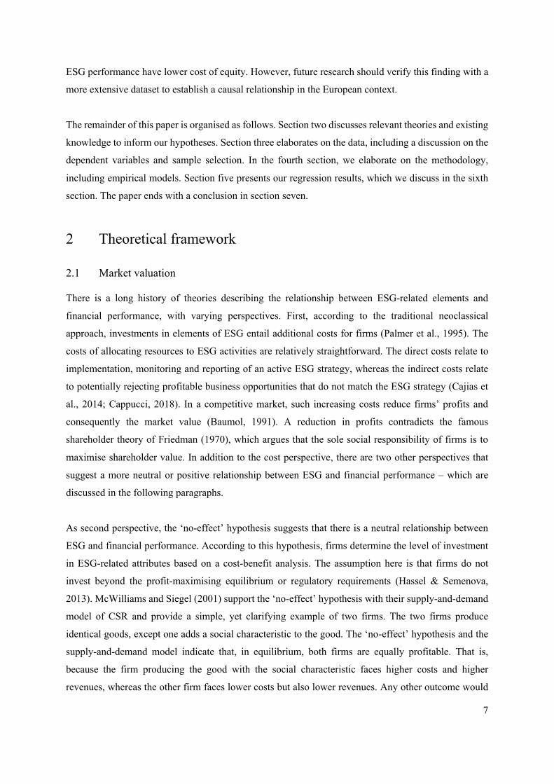
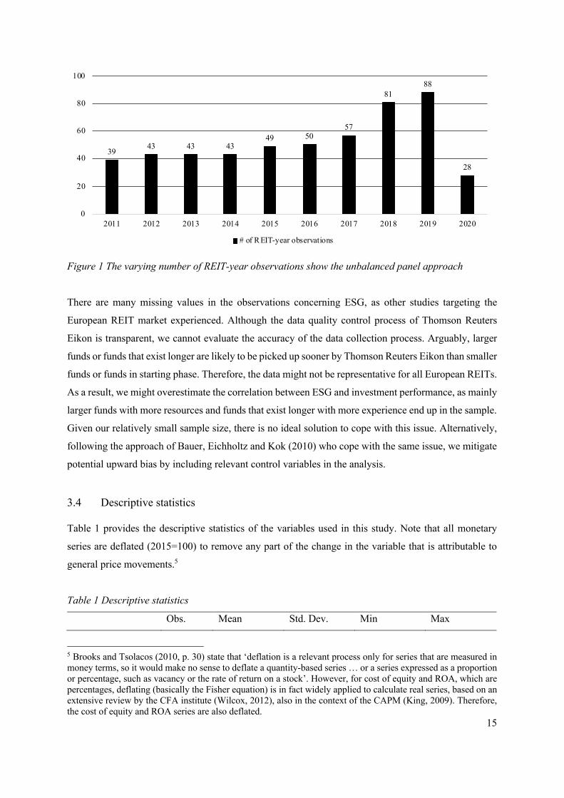
Figure 1 clearly illustrates the unbalanced panel approach, with a varying number of observations over
time. However, another issue the data suggest is increasing attention towards ESG over time, as the
number of REITs in the sample clearly increases over time. Thus, a potential learning effect might be
present in the data. A third observation is the huge drop in REIT-year observations in 2020. This is due
to the processing time of Thomson Reuters Eikon before the ratings are distributed.
15
Figure 1 The varying number of REIT-year observations show the unbalanced panel approach
There are many missing values in the observations concerning ESG, as other studies targeting the
European REIT market experienced. Although the data quality control process of Thomson Reuters
Eikon is transparent, we cannot evaluate the accuracy of the data collection process. Arguably, larger
funds or funds that exist longer are likely to be picked up sooner by Thomson Reuters Eikon than smaller
funds or funds in starting phase. Therefore, the data might not be representative for all European REITs.
As a result, we might overestimate the correlation between ESG and investment performance, as mainly
larger funds with more resources and funds that exist longer with more experience end up in the sample.
Given our relatively small sample size, there is no ideal solution to cope with this issue. Alternatively,
following the approach of Bauer, Eichholtz and Kok (2010) who cope with the same issue, we mitigate
potential upward bias by including relevant control variables in the analysis.
3.4 Descriptive statistics
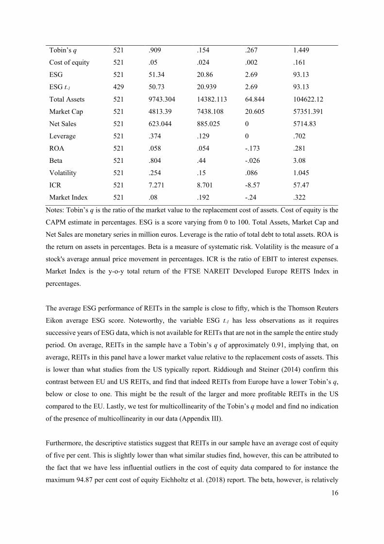
Table 1 provides the descriptive statistics of the variables used in this study. Note that all monetary
series are deflated (2015=100) to remove any part of the change in the variable that is attributable to
general price movements.5
Table 1 Descriptive statistics
Obs. Mean Std. Dev. Min Max
5 Brooks and Tsolacos (2010, p. 30) state that ‘deflation is a relevant process only for series that are measured in money terms, so it would make no sense to deflate a quantity-based series … or a series expressed as a proportion or percentage, such as vacancy or the rate of return on a stock’. However, for cost of equity and ROA, which are percentages, deflating (basically the Fisher equation) is in fact widely applied to calculate real series, based on an extensive review by the CFA institute (Wilcox, 2012), also in the context of the CAPM (King, 2009). Therefore, the cost of equity and ROA series are also deflated.
39 43 43 4349 50
57
8188
28
0
20
40
60
80
100
2011 2012 2013 2014 2015 2016 2017 2018 2019 2020
# of REIT-year observations
16
Tobin’s q 521 .909 .154 .267 1.449
Cost of equity 521 .05 .024 .002 .161
ESG 521 51.34 20.86 2.69 93.13
ESG t-1 429 50.73 20.939 2.69 93.13
Total Assets 521 9743.304 14382.113 64.844 104622.12
Market Cap 521 4813.39 7438.108 20.605 57351.391
Net Sales 521 623.044 885.025 0 5714.83
Leverage 521 .374 .129 0 .702
ROA 521 .058 .054 -.173 .281
Beta 521 .804 .44 -.026 3.08
Volatility 521 .254 .15 .086 1.045
ICR 521 7.271 8.701 -8.57 57.47
Market Index 521 .08 .192 -.24 .322
Notes: Tobin’s q is the ratio of the market value to the replacement cost of assets. Cost of equity is the
CAPM estimate in percentages. ESG is a score varying from 0 to 100. Total Assets, Market Cap and
Net Sales are monetary series in million euros. Leverage is the ratio of total debt to total assets. ROA is
the return on assets in percentages. Beta is a measure of systematic risk. Volatility is the measure of a
stock's average annual price movement in percentages. ICR is the ratio of EBIT to interest expenses.
Market Index is the y-o-y total return of the FTSE NAREIT Developed Europe REITS Index in
percentages.
The average ESG performance of REITs in the sample is close to fifty, which is the Thomson Reuters
Eikon average ESG score. Noteworthy, the variable ESG t-1 has less observations as it requires
successive years of ESG data, which is not available for REITs that are not in the sample the entire study
period. On average, REITs in the sample have a Tobin’s q of approximately 0.91, implying that, on
average, REITs in this panel have a lower market value relative to the replacement costs of assets. This
is lower than what studies from the US typically report. Riddiough and Steiner (2014) confirm this
contrast between EU and US REITs, and find that indeed REITs from Europe have a lower Tobin’s q,
below or close to one. This might be the result of the larger and more profitable REITs in the US
compared to the EU. Lastly, we test for multicollinearity of the Tobin’s q model and find no indication
of the presence of multicollinearity in our data (Appendix III).
Furthermore, the descriptive statistics suggest that REITs in our sample have an average cost of equity
of five per cent. This is slightly lower than what similar studies find, however, this can be attributed to
the fact that we have less influential outliers in the cost of equity data compared to for instance the
maximum 94.87 per cent cost of equity Eichholtz et al. (2018) report. The beta, however, is relatively
17
low with 0.8, suggesting REITs in the sample are less volatile than the market average. We suggest this
is due to the mainly larger funds in our sample, as the larger funds are more likely to report on ESG and
end up in the sample. As the beta (as risk measure) is also a factor in the cost of equity, the correlation
matrix (Appendix III) suggests high correlation. Therefore, we verify potential multicollinearity using
the Variance Inflation Factors (VIF), and find no multicollinearity issues (Table 8 in Appendix III).
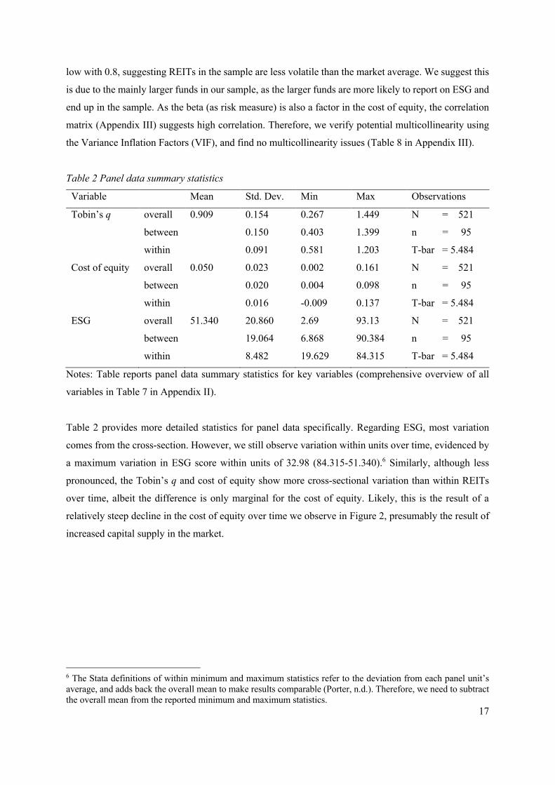
Table 2 Panel data summary statistics
Variable Mean Std. Dev. Min Max Observations
Tobin’s q overall
between
within
0.909 0.154
0.150
0.091
0.267
0.403
0.581
1.449
1.399
1.203
N = 521
n = 95
T-bar = 5.484
Cost of equity overall
between
within
0.050
0.023
0.020
0.016
0.002
0.004
-0.009
0.161
0.098
0.137
N = 521
n = 95
T-bar = 5.484
ESG overall
between
within
51.340 20.860
19.064
8.482
2.69
6.868
19.629
93.13
90.384
84.315
N = 521
n = 95
T-bar = 5.484
Notes: Table reports panel data summary statistics for key variables (comprehensive overview of all
variables in Table 7 in Appendix II).
Table 2 provides more detailed statistics for panel data specifically. Regarding ESG, most variation
comes from the cross-section. However, we still observe variation within units over time, evidenced by
a maximum variation in ESG score within units of 32.98 (84.315-51.340).6 Similarly, although less
pronounced, the Tobin’s q and cost of equity show more cross-sectional variation than within REITs
over time, albeit the difference is only marginal for the cost of equity. Likely, this is the result of a
relatively steep decline in the cost of equity over time we observe in Figure 2, presumably the result of
increased capital supply in the market.
6 The Stata definitions of within minimum and maximum statistics refer to the deviation from each panel unit’s average, and adds back the overall mean to make results comparable (Porter, n.d.). Therefore, we need to subtract the overall mean from the reported minimum and maximum statistics.
18
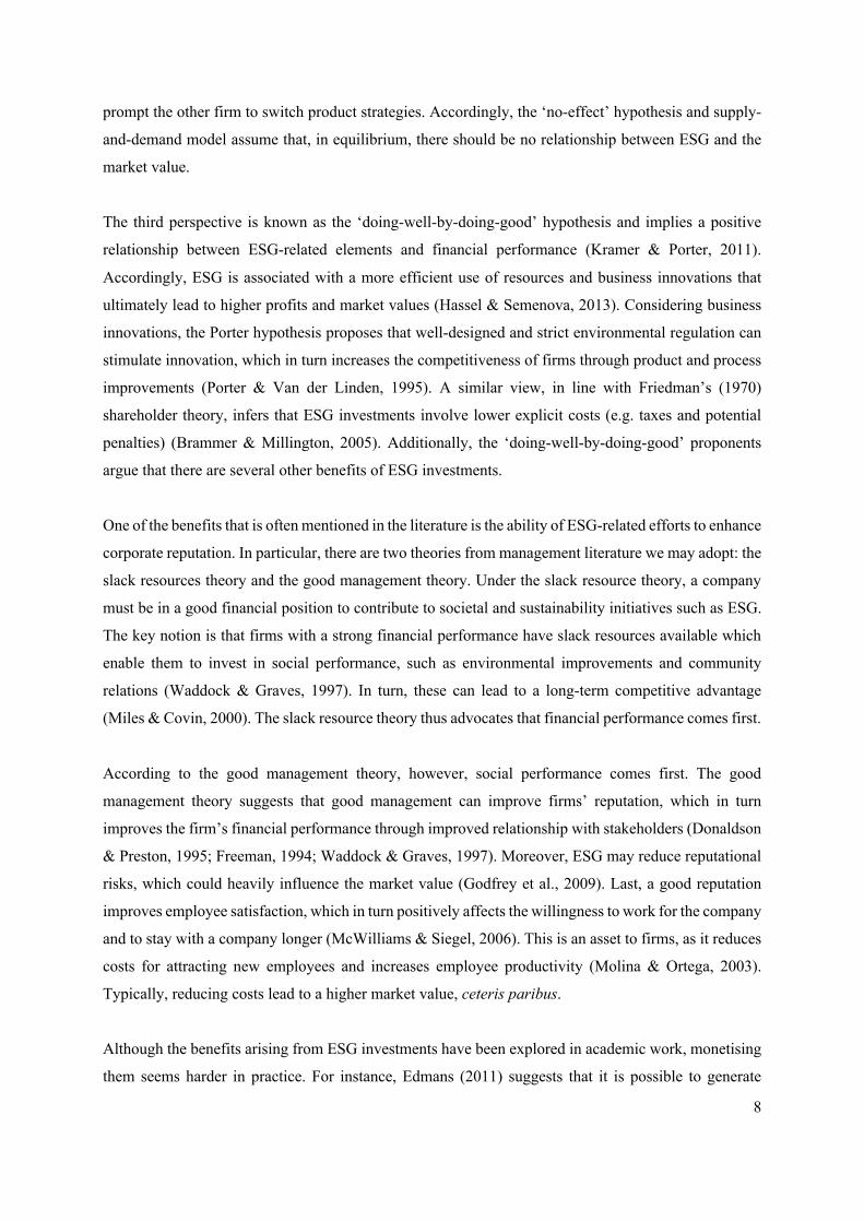
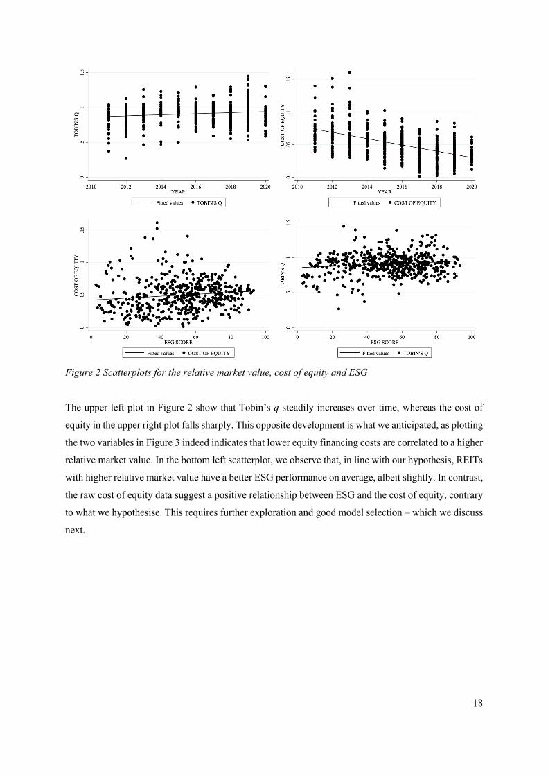
Figure 2 Scatterplots for the relative market value, cost of equity and ESG
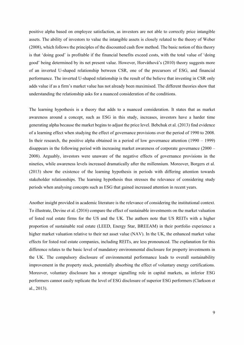
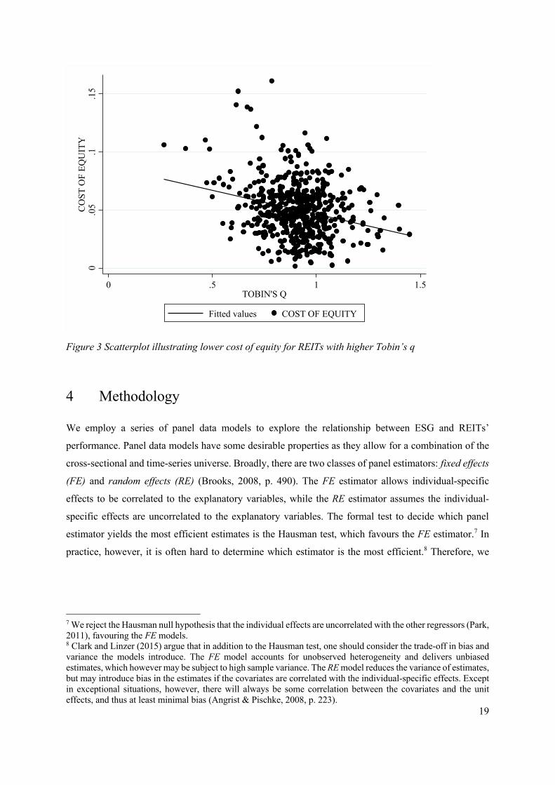
The upper left plot in Figure 2 show that Tobin’s q steadily increases over time, whereas the cost of
equity in the upper right plot falls sharply. This opposite development is what we anticipated, as plotting
the two variables in Figure 3 indeed indicates that lower equity financing costs are correlated to a higher
relative market value. In the bottom left scatterplot, we observe that, in line with our hypothesis, REITs
with higher relative market value have a better ESG performance on average, albeit slightly. In contrast,
the raw cost of equity data suggest a positive relationship between ESG and the cost of equity, contrary
to what we hypothesise. This requires further exploration and good model selection – which we discuss
next.
19
Figure 3 Scatterplot illustrating lower cost of equity for REITs with higher Tobin’s q
4 Methodology
We employ a series of panel data models to explore the relationship between ESG and REITs’
performance. Panel data models have some desirable properties as they allow for a combination of the
cross-sectional and time-series universe. Broadly, there are two classes of panel estimators: fixed effects
(FE) and random effects (RE) (Brooks, 2008, p. 490). The FE estimator allows individual-specific
effects to be correlated to the explanatory variables, while the RE estimator assumes the individual-
specific effects are uncorrelated to the explanatory variables. The formal test to decide which panel
estimator yields the most efficient estimates is the Hausman test, which favours the FE estimator.7 In
practice, however, it is often hard to determine which estimator is the most efficient.8 Therefore, we
7 We reject the Hausman null hypothesis that the individual effects are uncorrelated with the other regressors (Park, 2011), favouring the FE models. 8 Clark and Linzer (2015) argue that in addition to the Hausman test, one should consider the trade-off in bias and variance the models introduce. The FE model accounts for unobserved heterogeneity and delivers unbiased estimates, which however may be subject to high sample variance. The RE model reduces the variance of estimates, but may introduce bias in the estimates if the covariates are correlated with the individual-specific effects. Except in exceptional situations, however, there will always be some correlation between the covariates and the unit effects, and thus at least minimal bias (Angrist & Pischke, 2008, p. 223).
0.0
5.1
.15
CO
ST O
F EQ
UIT
Y
0 .5 1 1.5TOBIN'S Q
Fitted values COST OF EQUITY
20
follow Sah, Miller and Ghosh (2013) and estimate all models with both RE and FE to demonstrate the
robustness of our estimations.9
The relative market value and cost of equity we use to measure REIT performance, are explained by
different factors. Therefore, we need separate model specifications. In this section, we only discuss the
main model we take forward for each. In the results section, we gradually build up the models to
demonstrate the robustness of our estimates (Neumayer & Plümper, 2017, p. 133).
In the first stage of the analysis, we explore the correlation between ESG and the relative market value.
In constructing the model, we closely follow Cajias et al. (2014), and seek to improve their model by
increasing its explanatory power and reducing endogeneity concerns. First, we include the natural
logarithm of the book value of assets (Bauer et al., 2010; Shin & Stulz; 2000) and the natural logarithm
of the cost of equity, as literature (Riddiough & Steiner, 2014) and the preliminary analysis in the
previous section suggest a negative relationship. Second, we do not include contemporaneous and
lagged ESG performance simultaneously, but in separate model specifications rather. In the main model,
we include only the contemporaneous ESG performance, hence we specify the main model for the
relative market value as follows:
67( !")!# = α + 3$.,9!# + γ;!# + <# + δ! + θ# +ℇ!# (3)
Where 67( !")!# is the natural logarithm of Tobin’s q for REIT i in year t; α is the constant; ; is a vector
of REIT-level financial attributes for REIT i in year t, including market capitalisation, volatility, net
sales, leverage, total assets, and the cost of equity; <# is the FTSE NAREIT Developed Europe REITS
Index in year t to control for real estate market conditions; δ! are the REIT-specific dummies as this
specification represents the FE estimator; θ# are the dummies for years to control for a time trend10; and
ℇ!" is the error term for REIT i in year t.
Next, we introduce the main model we use to analyse the correlation between ESG and the cost of
equity. In deciding on which control variables to include, we closely follow Hsieh et al. (2020), who
enhance the model of Eichholtz et al. (2018) with the most recent insights on the determinants of the
9 As a final check before performing our regressions, we verify the presence of a panel effect in the FE model by conducting an F test and a Breusch-Pagan Lagrange multiplier (LM) test for the RE model, both comparing the panel estimator to a pooled ordinary least squares (OLS) regression (Clark & Linzer, 2015). We reject the null hypotheses of the F test and Breusch-Pagan LM test and assume panel estimators are the most efficient estimators. 10 We run the model with and without time fixed effects and use the Stata command testparm to analyse whether time fixed effects should be included in the FE model. We reject the null-hypothesis that the coefficients for all years are jointly equal to zero, therefore we need to control for a potential time trend by including time fixed effects.
21
cost of equity. However, we replace the market-to-book ratio in the Hsiesh et al. (2020) model with the
natural logarithm of Tobin’s q, as a more accurate measure of REIT value, leading to the following
specification:
67( &@.)!# = α + 3$.,9!# + γ;!# + δ! + θ# +ℇ!# (4)
Where 67( &@.)!# is the natural logarithm of the CAPM estimate of the cost of equity for REIT i in year
t; α is the constant; ; is a vector of REIT-level financial attributes for REIT i in year t, including return
on assets, total assets, leverage, Tobin’s q, interest coverage ratio and volatility; δ! are the REIT-specific
dummies, again as this specification represents the FE estimator; θ# are the year dummies to control for
a time trend 11; and ℇ!" is the error term for REIT i in year t.
Finally, an important consideration in financial and economic research is the presence of survivorship
bias. Survivorship bias is a statistical bias caused by not including all indicators of all funds in
performance studies, especially those that have failed (Zhou & Ziobrowski, 2009). We mitigate
survivorship bias in our methodology by applying an unbalanced panel approach, following Cajias et
al. (2014) and Devine et al. (2016). We carefully construct an unbalanced panel where REITs enter
when they first meet the data requirements and exit when they default or merge.
5 Results
5.1 Market valuation
Table 3 shows the results of the first stage of the analysis, in which we take a step-by-step approach and
test several variations of our main model to show the robustness of the results (Neumayer & Plümper,
2017, p. 133). We start with a baseline model and gradually add fixed effects to control for unobserved
heterogeneity related to REIT-level attributes, real estate market conditions and a general time trend,
and add lagged terms. The gradual development of the models enables us to observe the increase in
explanatory power of the models in terms of r-squared.12. All models, except the baseline model which
includes only the variable of interest, explain well over seventy per cent of the variance in the relative
market value.
11 We run the model with and without time fixed effects and use the Stata command testparm to analyse whether time fixed effects should be included in the FE model. We reject the null-hypothesis that the coefficients for all years are jointly equal to zero, therefore we need to control for a potential time trend by including time fixed effects. 12 The r-squared for FE models is typically lower, since variables are demeaned to obtain the FE within-estimator, leading to less total variance to be explained.
22
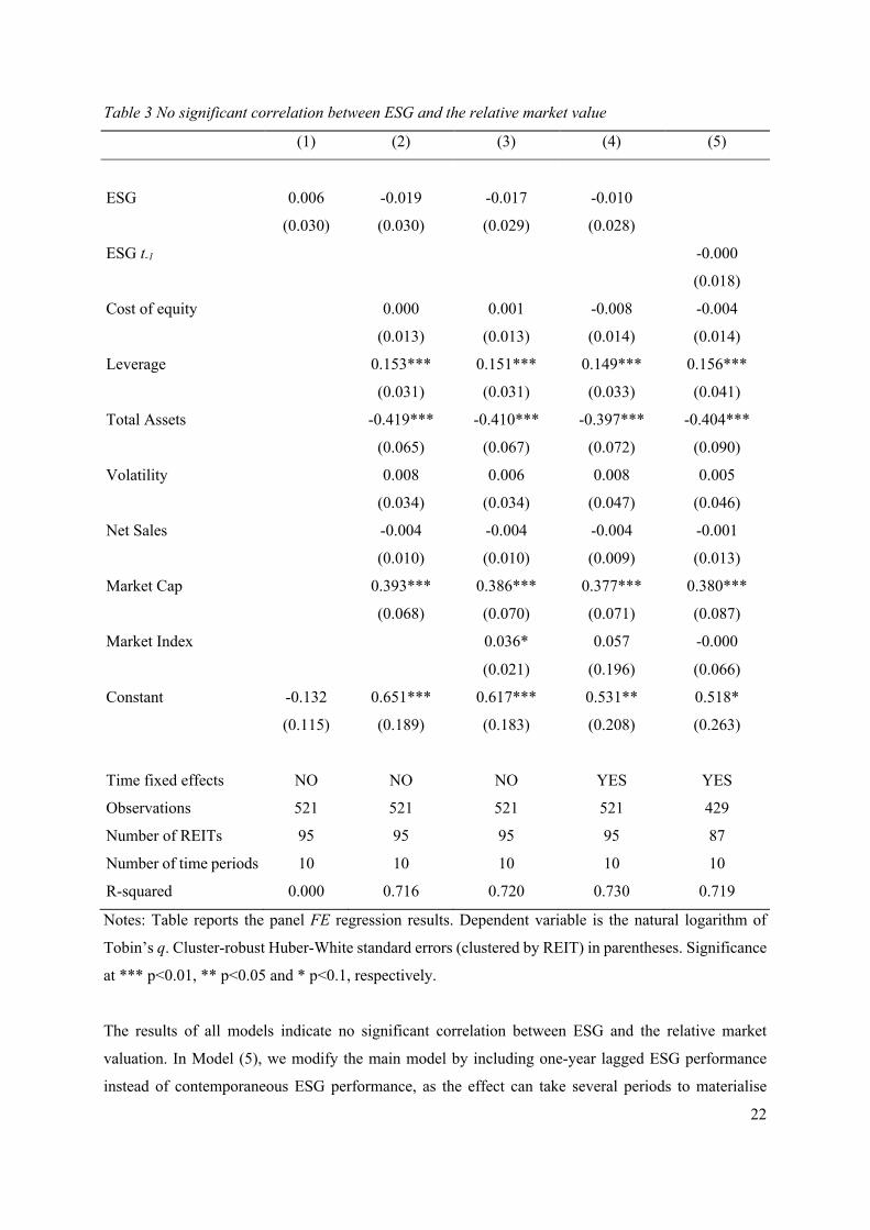
Table 3 No significant correlation between ESG and the relative market value
(1) (2) (3) (4) (5)
ESG 0.006 -0.019 -0.017 -0.010
(0.030) (0.030) (0.029) (0.028)
ESG t-1 -0.000
(0.018)
Cost of equity 0.000 0.001 -0.008 -0.004
(0.013) (0.013) (0.014) (0.014)
Leverage 0.153*** 0.151*** 0.149*** 0.156***
(0.031) (0.031) (0.033) (0.041)
Total Assets -0.419*** -0.410*** -0.397*** -0.404***
(0.065) (0.067) (0.072) (0.090)
Volatility 0.008 0.006 0.008 0.005
(0.034) (0.034) (0.047) (0.046)
Net Sales -0.004 -0.004 -0.004 -0.001
(0.010) (0.010) (0.009) (0.013)
Market Cap 0.393*** 0.386*** 0.377*** 0.380***
(0.068) (0.070) (0.071) (0.087)
Market Index 0.036* 0.057 -0.000
(0.021) (0.196) (0.066)
Constant -0.132 0.651*** 0.617*** 0.531** 0.518*
(0.115) (0.189) (0.183) (0.208) (0.263)
Time fixed effects NO NO NO YES YES
Observations 521 521 521 521 429
Number of REITs 95 95 95 95 87
Number of time periods 10 10 10 10 10
R-squared 0.000 0.716 0.720 0.730 0.719
Notes: Table reports the panel FE regression results. Dependent variable is the natural logarithm of
Tobin’s q. Cluster-robust Huber-White standard errors (clustered by REIT) in parentheses. Significance
at *** p<0.01, ** p<0.05 and * p<0.1, respectively.
The results of all models indicate no significant correlation between ESG and the relative market
valuation. In Model (5), we modify the main model by including one-year lagged ESG performance
instead of contemporaneous ESG performance, as the effect can take several periods to materialise
23
(Cajias et al., 2014). The consideration to lag the performance by only one year lies in the concept of
the ESG rating. The contemporaneous rating is in fact already partially lagged, as we observe in the
number of REIT-year observations over time (Figure 1) that it takes Thomson Reuters time to construct
and distribute the ESG ratings.
However, including lagged ESG performance reduces the number of observations compared to the other
models, as it requires longer time series that are not available. As such, the estimates of Model (5) might
be driven by the change in sample rather than the substitution of lagged for contemporaneous ESG
performance. Therefore, we re-estimate all models with a constant sample, and find consistent results
(see Table 18 in Appendix V). Additionally, we provide several robustness checks by conducting a first
difference (FD) approach13 following Cajias et al. (2014) and Eichholtz et al. (2018), re-estimating all
models using the RE estimator following Sah et al. (2013), and different methodologies to estimate the
dependent variable Tobin’s q. The estimates of the robustness checks are consistent with the original
estimates.
Still, some previous studies indicate a significant effect of ESG-related performance on the market value
(Cajias et al., 2014; Devine et al., 2016), albeit slightly (Sah et al., 2013). A potential explanation relates
to the period covered in these studies, as the learning hypothesis suggests the level of attention towards
ESG might affect the correlation. Hence, we split up the original sample into two time periods covering
2011 – 2015 and 2016 – 2020, based on the increased attention towards ESG following the Paris
Agreement in 2015. The results in Appendix V (Table 22) suggest the presence of a learning effect, as
the initial insignificant estimate for ESG holds for 2011 – 2015, but becomes significant at the one per
cent level for 2016 – 2020. Interestingly, the negative coefficient suggests that a one per cent increase
in ESG is correlated with a 0.032 per cent lower Tobin’s q, ceteris paribus.
Another issue that could clarify the insignificant correlation found in the original model is the proxy for
sustainability Devine et al. (2016) use (green building certifications). Arguably, the benefits of green
building certifications are clearest to investors as this comes closest to ‘traditional’ sustainability. In
contrast, we use the broader ESG concept as sustainability proxy including intangible benefits. What
we already know from literature, is that investors might not be able to correctly price such intangible
assets (Edmans, 2011). It is therefore interesting to explore whether this impacts our estimates and
13 As a first robustness check to account for unobserved heterogeneity in an alternative way compared to the FE estimators, we also estimate a FD model. Under the same assumptions as the FE model, both the FE and FD estimators are consistent. However, the FD model picks up only the instantaneous effect at time t of our variable of interest "#$ on %&'()#*,. It is likely, however, that the effect of ESG needs several periods to materialise, for which the FE estimator picks up the average. We find that the insignificant relationship for contemporary ESG performance in the FE models is consistent with the FD model, which provides an insignificant coefficient of -0.007 (see Table 20 in Appendix V).
24
explains the insignificant results. We do so by decomposing comprehensive ESG performance into
separate pillars (E, S and G) and present results in Appendix VI (Table 25).
The decomposing exercise does not provide evidence that the ability of investors to value the intangibles
influenced our estimates of ESG for the relative market value, as the separate pillars (E, S and G) are all
insignificant. However, we also explored the correlation of the separate pillars for the cost of equity
(Table 26). Remarkably, the environmental and social pillar are significant at the one per cent level,
whereas the governance metric is insignificant. A potential explanation for the absence of a governance
correlation is that REITs in developed countries are typically subject to strict governance regulations to
obtain – and maintain – their REIT status (EPRA, 2020). Consequently, there might be a baseline level
of governance structure among all REITs, such that capital market participants place less value on
superior governance performance. In conclusion, the absent governance correlation may explain the
presence of a sustainability-related effects found in studies that exclusively focus on the environmental
aspect (Devine et al., 2016).
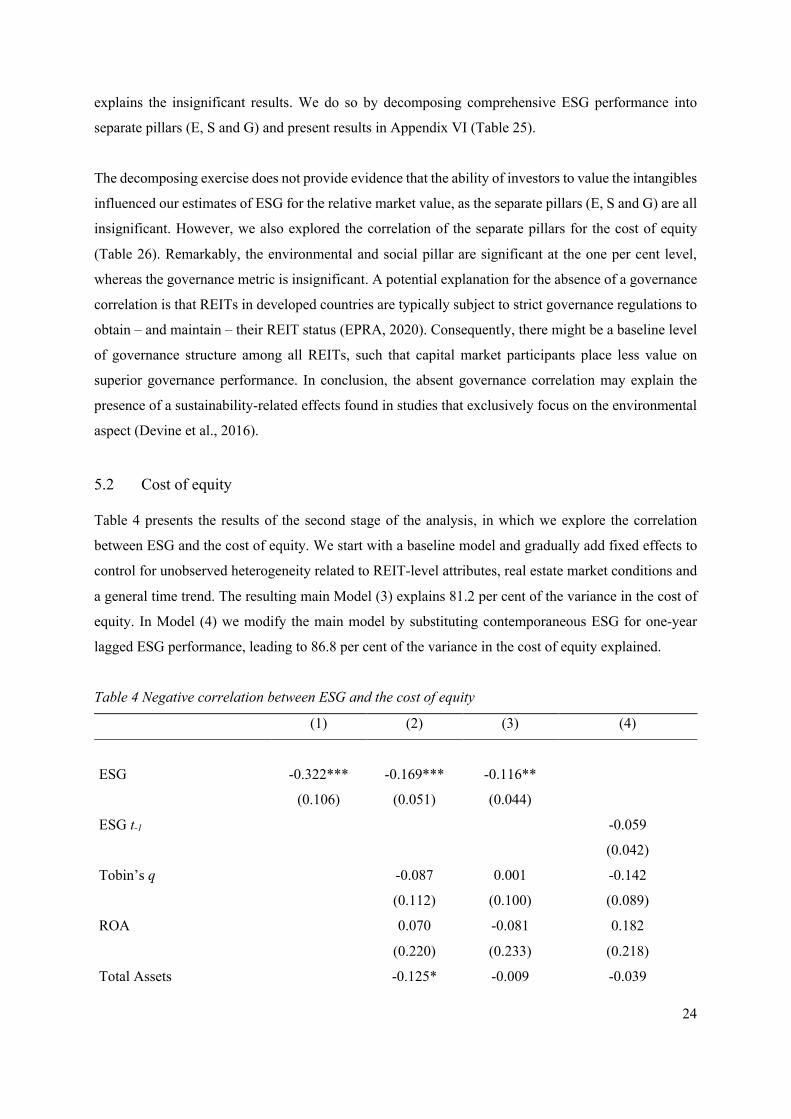
5.2 Cost of equity
Table 4 presents the results of the second stage of the analysis, in which we explore the correlation
between ESG and the cost of equity. We start with a baseline model and gradually add fixed effects to
control for unobserved heterogeneity related to REIT-level attributes, real estate market conditions and
a general time trend. The resulting main Model (3) explains 81.2 per cent of the variance in the cost of
equity. In Model (4) we modify the main model by substituting contemporaneous ESG for one-year
lagged ESG performance, leading to 86.8 per cent of the variance in the cost of equity explained.
Table 4 Negative correlation between ESG and the cost of equity
(1) (2) (3) (4)
ESG -0.322*** -0.169*** -0.116**
(0.106) (0.051) (0.044)
ESG t-1 -0.059
(0.042)
Tobin’s q -0.087 0.001 -0.142
(0.112) (0.100) (0.089)
ROA 0.070 -0.081 0.182
(0.220) (0.233) (0.218)
Total Assets -0.125* -0.009 -0.039
25
(0.064) (0.076) (0.071)
Leverage 0.124*** 0.046 0.114*
(0.047) (0.055) (0.057)
Beta 1.207*** 1.261*** 1.269***
(0.112) (0.120) (0.119)
ICR 0.000 0.001 0.002
(0.002) (0.002) (0.002)
Volatility -1.034*** -1.642*** -1.583***
(0.305) (0.436) (0.433)
Constant -1.908*** -2.033*** -2.952*** -2.912***
(0.406) (0.541) (0.538) (0.562)
Time fixed effects NO NO YES YES
Observations 521 521 521 429
Number of REITs 95 95 95 87
Number of time periods 10 10 10 10
R-squared 0.053 0.773 0.812 0.868
Notes: Table reports the panel FE regression results. Dependent variable is the natural logarithm of the
cost of equity. Cluster-robust Huber-White standard errors (clustered by REIT) in parentheses.
Significance at *** p<0.01, ** p<0.05 and * p<0.1, respectively.
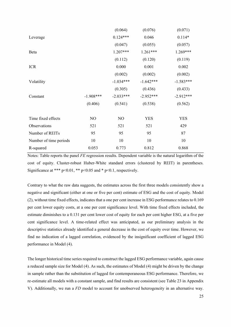
Contrary to what the raw data suggests, the estimates across the first three models consistently show a
negative and significant (either at one or five per cent) estimate of ESG and the cost of equity. Model
(2), without time fixed effects, indicates that a one per cent increase in ESG performance relates to 0.169
per cent lower equity costs, at a one per cent significance level. With time fixed effects included, the
estimate diminishes to a 0.131 per cent lower cost of equity for each per cent higher ESG, at a five per
cent significance level. A time-related effect was anticipated, as our preliminary analysis in the
descriptive statistics already identified a general decrease in the cost of equity over time. However, we
find no indication of a lagged correlation, evidenced by the insignificant coefficient of lagged ESG
performance in Model (4).
The longer historical time series required to construct the lagged ESG performance variable, again cause
a reduced sample size for Model (4). As such, the estimates of Model (4) might be driven by the change
in sample rather than the substitution of lagged for contemporaneous ESG performance. Therefore, we
re-estimate all models with a constant sample, and find results are consistent (see Table 23 in Appendix
V). Additionally, we run a FD model to account for unobserved heterogeneity in an alternative way.
26
The negative correlation found in the original model is consistent with the FD model, which provides a
coefficient of -0.052, significant at five per cent (Table 21 in Appendix V). The lower coefficient of the
FD model can be explained by the fact that the FD model picks up only the instantaneous effect of ESG
performance at time t, while the FE estimator picks up an average over time through demeaning. Finally,
we re-estimate all models using the RE estimator instead of the FE estimator, following Sah et al. (2013).
The sign and significance are broadly similar, albeit the coefficient of Model (3) is insignificant.
However, as the other robustness checks point towards a negative correlation, we consider the original
estimates largely robust to the choice of estimator.
As with the relative market valuation, we split up the sample into two periods to test whether the
increased attention towards ESG in recent years influences our estimates. Interestingly, the results in
Appendix V (Table 22) show no significant correlation in the period 2011 – 2015, whereas the
coefficient (-0.155) of ESG in 2016 – 2020 is significant at the five per cent level.
The empirical results imply that ESG performance is related to lower equity costs, contrary to what raw
data suggests. A first line of reasoning emphasises the importance of a good model to control for
characteristics and a time trend. At the same time, we put a lot of trust in our models. However, given
the high goodness-of-fit measure, the expected negative correlation based on theory, and the fact that
we closely followed existing empirical work in our model construction (Eichholtz et al., 2018; Hsieh et
al., 2020), we believe the empirical results reflect the actual correlation better than the raw data.
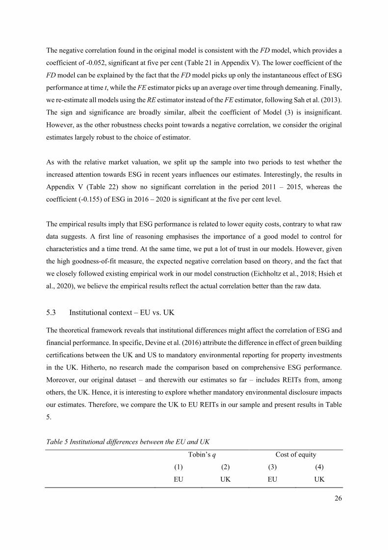
5.3 Institutional context – EU vs. UK
The theoretical framework reveals that institutional differences might affect the correlation of ESG and
financial performance. In specific, Devine et al. (2016) attribute the difference in effect of green building
certifications between the UK and US to mandatory environmental reporting for property investments
in the UK. Hitherto, no research made the comparison based on comprehensive ESG performance.
Moreover, our original dataset – and therewith our estimates so far – includes REITs from, among
others, the UK. Hence, it is interesting to explore whether mandatory environmental disclosure impacts
our estimates. Therefore, we compare the UK to EU REITs in our sample and present results in Table
5.
Table 5 Institutional differences between the EU and UK
Tobin’s q Cost of equity
(1) (2) (3) (4)
EU UK EU UK
27
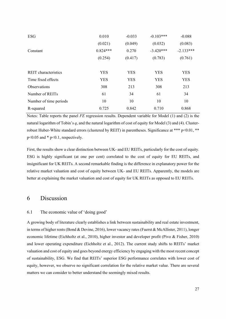
ESG 0.010 -0.033 -0.103*** -0.088
(0.021) (0.049) (0.032) (0.083)
Constant 0.824*** 0.270 -3.420*** -2.133***
(0.254) (0.417) (0.783) (0.761)
REIT characteristics YES YES YES YES
Time fixed effects YES YES YES YES
Observations 308 213 308 213
Number of REITs 61 34 61 34
Number of time periods 10 10 10 10
R-squared 0.725 0.842 0.710 0.868
Notes: Table reports the panel FE regression results. Dependent variable for Model (1) and (2) is the
natural logarithm of Tobin’s q, and the natural logarithm of cost of equity for Model (3) and (4). Cluster-
robust Huber-White standard errors (clustered by REIT) in parentheses. Significance at *** p<0.01, **
p<0.05 and * p<0.1, respectively.
First, the results show a clear distinction between UK- and EU REITs, particularly for the cost of equity.
ESG is highly significant (at one per cent) correlated to the cost of equity for EU REITs, and
insignificant for UK REITs. A second remarkable finding is the difference in explanatory power for the
relative market valuation and cost of equity between UK- and EU REITs. Apparently, the models are
better at explaining the market valuation and cost of equity for UK REITs as opposed to EU REITs.
6 Discussion
6.1 The economic value of ‘doing good’
A growing body of literature clearly establishes a link between sustainability and real estate investment,
in terms of higher rents (Bond & Devine, 2016), lower vacancy rates (Fuerst & McAllister, 2011), longer
economic lifetime (Eichholtz et al., 2010), higher investor and developer profit (Pivo & Fisher, 2010)
and lower operating expenditure (Eichholtz et al., 2012). The current study shifts to REITs’ market
valuation and cost of equity and goes beyond energy efficiency by engaging with the most recent concept
of sustainability, ESG. We find that REITs’ superior ESG performance correlates with lower cost of
equity, however, we observe no significant correlation for the relative market value. There are several
matters we can consider to better understand the seemingly mixed results.
28
First, the absence of significant correlation of ESG and relative market value might indicate a mixed
presence of ‘cost perspective’- and ‘doing-well-by-doing-good’ proponents among European REIT
investors, as suggested by Eom and Nam (2017). Second, the ‘no-effect’ hypothesis may apply, where
the costs and benefits arising from ESG cancel out (Hassel & Semenova, 2013; McWilliams & Siegel,
2001). Still, however, along these lines, one would expect to see similar result for the cost of equity.
Moreover, in a competitive market, lower cost (of equity) should lead to a higher market value
(Riddiough & Steiner, 2014). Therefore, as third consideration, we disentangle the measure of market
value. The Tobin’s q is considered the market value (numerator) over the asset replacement costs
(denominator). Potentially, the replacement costs of assets (denominator) increase beyond the market
value (numerator) with ESG performance, stabilising the relative market value and blurring potential
correlation.
6.2 Institutional context and transparency – its implications
This study contributes to literature by providing insight in ESG and REITs’ performance in Europe,
whereas nearly all existing studies target the US REIT market (Brounen & Marcato, 2018; Cajias et al.,
2014; Coën et al., 2018; Devine et al., 2016; Eichholtz et al., 2012; Fuerst, 2015; Sah et al., 2013). As
ESG data availability in Europe strongly increased in recent years, we are able to explore how ESG is
linked to the real estate investment market in Europe. In doing so, we present initial evidence that
institutional context matters for ESG in Europe. We find a significant correlation for ESG and the cost
of equity in the EU, which disappears in the UK where there is a mandatory level of environmental
reporting. Arguably, the upside of mandatory reporting is that it increases overall environmental
performance, as REITs with poor environmental performance cannot shy away. However,
simultaneously, the baseline level of reporting might mitigate the presence of a correlation between
voluntary ESG efforts and the cost of equity – or market value. An important remark with this finding,
is that we group all EU REITs and compare those to the UK REITs, as data limitations do not allow us
to dig deeper into the sample. However, this experiment could be enhanced in future research by
explicitly taking country-specific regulations into account for all countries in the sample.
6.3 The future of ESG in real estate investments
In this study, we find that there is an insignificant correlation between ESG and the market value and
cost of equity in the period 2011 – 2015, while there is a significant correlation in the more recent time
frame 2016 – 2020. Based on the literature there are two possible explanations. First, reasoning from
the learning hypothesis, the increased attention for ESG in recent years has increased investor
awareness, which in turn caused market to adjust price levels (Bebchuk et al., 2013). The second
perspective may stem from a ‘reap what you sow’ principle regarding ESG strategies. In the context of
29
ESG and REIT investment, there may be high upfront costs associated with ESG adoption, such as
strategy implementing costs or retrofitting assets (Cappucci, 2018), but arguably also future benefits
such as lower operating costs of assets or productivity improvements (Hassel & Semenova, 2013; Porter
& Van der Linden, 1995). Possibly, REITs have taken on the majority of the upfront costs in the 2011
– 2015 period, decreasing their performance in that time frame, while enjoying some of the benefits in
the more recent 2015 – 2020 time frame. Nevertheless, with this finding we agree with the accurate
statement of Brounen et al. (2021) that research on ESG becomes dates quickly, and see this as an
implication to frequently review the sign and significance of the correlation between ESG and REIT
performance.
As for the future of REIT research, our results might be affected by the availability of historical data,
reflected by relatively short time series. Moreover, the unbalanced sample approach we apply mitigates
survivalship bias, but results in some funds being included, for instance, for only two years, preventing
us from detecting potential inconsistencies. Therefore, it would be interesting to see whether the results
are stable over longer time periods in future research. Additionally, regarding the cross-sectional
element, we are unsure about the data collection process of Thomson Reuters Eikon as ESG data
provider. Comparing data providers would give more insight in the representativeness of the data for
European REITs and enhance reliability of the results – something future research could address.
7 Conclusion
In this study, we examined whether ESG performance is correlated with REITs’ market value and cost
of equity in the relatively unexplored European framework. We observe no correlation for REITs’
relative market value, but we find that ESG performance is negatively correlated with the cost of equity.
In contrast, when there is a mandatory level of environmental reporting for property investments present,
the correlation disappears. As such, the results underline the importance of considering the institutional
context for the correlation between ESG and real estate investments. However, future research should
verify these findings with a more comprehensive dataset to establish a causal relationship in the
European context.
30
References
An, X., & Pivo, G. (2020). Green buildings in commercial mortgage‐backed securities: The effects of
LEED and energy star certification on default risk and loan terms. Real Estate Economics, 48(1), 7-42.
Angrist, J. D., & Pischke, J. S. (2008). Mostly harmless econometrics. Princeton university press.
Bassen, A., Meyer, K., Hölz, H. M., Zamostny, A., & Schlange, J. (2006). The Influence of Corporate
Responsibility on the Cost of Capital–An Empirical Analysis 2006 [online]. https://www.schlange-
co.com/wp-content/uploads/2017/11/SchlangeCo_2006_CostOfCapital.pdf
Battese, G. E., & Coelli, T. J. (1995). A model for technical inefficiency effects in a stochastic frontier
production function for panel data. Empirical economics, 20(2), 325-332.
Bauer, R., Eichholtz, P., & Kok, N. (2010). Corporate governance and performance: The REIT effect.
Real estate economics, 38(1), 1-29.
Baumol, W., (1991), Perfect Markets and Easy Virtue: Business Ethics and the Invisible Hand, Basil
Blackwell, Oxford.
Bebchuk, L. A., Cohen, A., & Wang, C. C. (2013). Learning and the disappearing association between
governance and returns. Journal of Financial Economics, 108(2), 323-348.
Berk, J., DeMarzo, P., Harford, J., 2019. Fundamentals of Corporate Finance. Global Edition (Fourth
Edition). Harlow, England: Pearson.
Bond, S. A., & Devine, A. (2016). Certification matters: is green talk cheap talk?. The Journal of Real
Estate Finance and Economics, 52(2), 117-140.
Borgers, A., Derwall, J., Koedijk, K., & Ter Horst, J. (2013). Stakeholder relations and stock returns:
On errors in investors' expectations and learning. Journal of Empirical Finance, 22, 159-175.
Brammer, S., & Millington, A. (2005). Corporate reputation and philanthropy: An empirical analysis.
Journal of Business Ethics, 61(1), 29–44.
Brooks, C. (2008). Introductory Econometrics for Finance. Cambridge University Press.
31
Brooks, C., & Tsolacos, S. (2010). Real estate modelling and forecasting. Cambridge University Press.
Brounen, D., & Marcato, G. (2018). Sustainable Insights in Public Real Estate Performance: ESG Scores
and Effects in REIT Markets. Berkeley Lab.: Berkeley, CA, USA.
Brounen, D., Marcato, G., & Op’t Veld, H. (2021). Pricing ESG equity ratings and underlying data in
listed real estate securities. Sustainability, 13(4), 2037.
Cajias, M., Fuerst, F., & Bienert, S. (2012). Can Investing in Corporate Social Responsibility Lower a
Company’s Cost of Capital?. Available at SSRN 2157184.
Cajias, M., Fuerst, F., McAllister, P., & Nanda, A. (2014). Do responsible real estate companies
outperform their peers?. International Journal of Strategic Property Management, 18(1), 11-27.
Cappucci, M. (2018). The ESG integration paradox. Journal of Applied Corporate Finance, 30(2), 22-
28.
Clark, T., & Linzer, D. (2015). Should I Use Fixed or Random Effects? Political Science Research and
Methods, 3(2), 399-408. doi:10.1017/psrm.2014.32
Clarkson, P. M., Fang, X., Li, Y., & Richardson, G. (2013). The relevance of environmental disclosures:
Are such disclosures incrementally informative?. Journal of Accounting and Public Policy, 32(5), 410-
431.
Cohen, J., Holder-Webb, L., Nath, L., & Wood, D. (2011). Retail investors’ perceptions of the decision-
usefulness of economic performance, governance, and corporate social responsibility
disclosures. Behavioral Research in Accounting, 23(1), 109-129.
Damodaran, A. (2008). What is the riskfree rate? A Search for the Basic Building Block. A Search for
the Basic Building Block (December 14, 2008).
Derwall, J., Koedijk, K., & Ter Horst, J. (2011). A tale of values-driven and profit-seeking social
investors. Journal of Banking & Finance, 35(8), 2137-2147.
32
Devine, A., Steiner, E., & Yönder. C. E. (2016). Decomposing the value effects of sustainable
investment. Working Paper.
Dhaliwal, D. S., Li, O. Z., Tsang, A., & Yang, Y. G. (2011). Voluntary nonfinancial disclosure and the
cost of equity capital: The initiation of corporate social responsibility reporting. The accounting
review, 86(1), 59-100.
Donaldson, T., & Preston, L. E. (1995). The stakeholder theory of the corporation: Concepts,
evidence, and implications. Academy of management Review, 20(1), 65-91.
Drukker, D. M. 2003. Testing for serial correlation in linear panel-data models. The Stata Journal (3)2,
1-10.
Edmans, A. (2011). Does the stock market fully value intangibles? Employee satisfaction and equity
prices. Journal of Financial Economics, (101) 621-640.
Eichholtz, P., Kok, N., & Quigley, J. M. (2010). Doing well by doing good? Green office buildings.
American Economic Review, 100(5), 2492-2509.
Eichholtz, P., Kok, N., & Yonder, E. (2012). Portfolio greenness and the financial performance of
REITs. Journal of International Money and Finance, 31(7), 1911-1929.
Eichholtz, P., Barron, P., & Yönder, E. (2018). Sustainable REITs: REIT environmental performance
and the cost of equity. In The Routledge REITs Research Handbook (pp. 77-94). Routledge.
Eichholtz, P., Holtermans, R., Kok, N., & Yönder, E. (2019). Environmental performance and the cost
of debt: Evidence from commercial mortgages and REIT bonds. Journal of Banking & Finance, 102,
19-32.
El Ghoul, S., Guedhami, O., Kwok, C. C., & Mishra, D. R. (2011). Does corporate social
responsibility affect the cost of capital?. Journal of Banking & Finance, 35(9), 2388-2406.
Endrikat, J., Guenther, E., & Hoppe, H. (2014). Making sense of conflicting empirical findings: A
meta-analytic review of the relationship between corporate environmental and financial
performance. European Management Journal, 32(5), 735-751.
33
Eom, K., & Nam, G. (2017). Effect of Entry into Socially Responsible Investment Index on Cost of
Equity and Firm Value. Sustainability, 9(5), 717.
EPRA. (2021). Sustainable finance [online]. Retrieved from:
https://www.epra.com/sustainability/sustainability-regulation/sustainable-finance
Fatemi, A., Glaum, M., & Kaiser, S. (2018). ESG performance and firm value: The moderating role of
disclosure. Global Finance Journal, 38, 45-64.
Feri. (2009). Nachhaltige Investments Und Nachhaltigkeitsfonds Aus Anlegerperspektive – Studie 2009
(Feri Euro Rating Services). Bad Homburg.
Freeman, R. E. (1994). The politics of stakeholder theory: Some future directions. Business ethics
quarterly, 409-421.
Friede, G., Busch, T., & Bassen, A. (2015). ESG and financial performance: aggregated evidence from
more than 2000 empirical studies. Journal of Sustainable Finance & Investment, 5(4), 210-233.
Friedman, M. (1970). The social responsibility of business is to increase its profits. New York Times
Magazine, September 13: 32-33, 122-124.
Fuerst, F., & McAllister, P. (2011). The impact of Energy Performance Certificates on the rental and
capital values of commercial property assets. Energy policy, 39(10), 6608-6614.
Fuerst, F. (2015). The financial rewards of sustainability: A global performance study of real estate
investment trusts. Available at SSRN 2619434.
Fuerst, F., Gabrieli, T., & McAllister, P. (2017). A green winner's curse? Investor behavior in the market
for eco-certified office buildings. Economic Modelling, 61, 137-146.
Godfrey, P.C., Merrill, C.B., and Hansen, J.M., (2009), “The relationship between corporate social
responsibility and shareholder value: An empirical test of the risk management hypothesis”, Strategic
Management Journal, 30, 425-445.
Goss, A., & Roberts, G. S. (2011). The impact of corporate social responsibility on the cost of bank
loans. Journal of Banking & Finance, 35(7), 1794-1810.
34
Greene, W. H. (2000). Econometric analysis 4th edition. International edition, New Jersey: Prentice
Hall, 201-215.
Han, B. (2006). Insider ownership and firm value: evidence from real estate investment trusts. The
Journal of Real Estate Finance and Economics, 32(4), 471-493.
Hassel, L. G., & Semenova, N. (2013). The added value of ESG/SRI on company and portfolio levels–
What can we learn from research. CSR and beyond–A Nordic perspective, 137-163.
Heinkel, R., Kraus, A., & Zechner, J. (2001). The effect of green investment on corporate
behavior. Journal of financial and quantitative analysis, 36(4), 431-449.
Horváthová, E. (2010). Does environmental performance affect financial performance? A meta-
analysis. Ecological Economics, 70(1), 52-59.
Hsieh, H. C., Claresta, V., & Bui, T. M. N. (2020). Green building, cost of equity capital and corporate
governance: Evidence from us real estate investment trusts. Sustainability, 12(9), 3680.
King, M. R. (2009). The cost of equity for global banks: a CAPM perspective from 1990 to 2009. BIS
Quarterly Review, September.
Konar, S., & Cohen, M. A. (2001). Does the market value environmental performance? Review of
economics and statistics, 83(2), 281-289.
Kramer, M. R., & Porter, M. (2011). Creating shared value (Vol. 17). FSG.
Lang, L. H., & Stulz, R. M. (1994). Tobin's q, corporate diversification, and firm
performance. Journal of political economy, 102(6), 1248-1280.
Levin, A., Lin, C. F., & Chu, C. S. J. (2002). Unit root tests in panel data: asymptotic and finite-sample
properties. Journal of econometrics, 108(1), 1-24.
Lindenberg, E. B., & Ross, S. A. (1981). Tobin's q ratio and industrial organization. Journal of
business, 1-32.
35
Mackey, A., Mackey, T. B., & Barney, J. B. (2007). Corporate social responsibility and firm
performance: Investor preferences and corporate strategies. Academy of management review, 32(3),
817-835.
Mariani, M., Amoruso, P., Caragnano, A., & Zito, M. (2018). Green real estate: does it create value?
Financial and sustainability analysis on European green REITs. International Journal of Business and
Management, 13, 80-92.
McWilliams, A., Siegel, D.S., Wrights, P.V., (2006) Corporate social responsibility: strategic
implications. Journal of Management Studies, 43(1), 1-18.
Molina, J. A., & Ortega, R. (2003). Effects of employee training on the performance of North-American
firms. Applied Economics Letters, 10(9), 549-552.
Morri, G., Anconetani, R., & Benfari, L. (2020). Greenness and financial performance of European
REITs. Journal of European Real Estate Research.
Neumayer, E., & Plümper, T. (2017). Robustness tests for quantitative research. Cambridge University
Press.
Nikolaev, V., & Van Lent, L. (2005). The endogeneity bias in the relation between cost-of-debt capital
and corporate disclosure policy. European Accounting Review, 14(4), 677-724.
Palmer, K., Oates, W.E., Portey, P.R., (1995), Tightening environmental standards: the benefit-cost or
the no-cost paradigm? Journal of Economic Perspectives, 9(4), 119-132.
Park, H.M. (2011). Practical Guides To Panel Data Modeling: A Step-by-step Analysis Using Stata.
Tutorial Working Paper. Graduate School of International Relations, International University of Japan.
Perfect, S. B., & Wiles, K. W. (1994). Alternative constructions of Tobin's q: An empirical comparison.
Journal of empirical finance, 1(3-4), 313-341.
Pivo, G., & Fisher, J. (2010). Income, value, and returns in socially responsible office properties.
Journal of real Estate research, 32(3), 243-270.
Porter, M. and Van der Linde, C. (1995) Toward a new conception of the environment-competitiveness
36
relationship, The Journal of Economic Perspectives, 9(4), 97-118.
Porter, S. (n.d.). Xtsum handout [online]. Retrieved from.
http://stephenporter.org/files/xtsum_handout.pdf
Refinitiv. (2019). Refinitiv Eikon – your trusted source of financial analysis data and tools [Brochure].
https://www.refinitiv.com/content/dam/marketing/en_us/documents/brochures/eikon-overview-
brochure.pdf
Riddiough, T., & Steiner, E. (2014). Capital structure and firm performance. EPRA Research.
https://prodapp.epra.com/media/Capital_structure_and_firm_performance_-
_EPRA_research_1422012104292.pdf
Riedl, A., & Smeets, P. (2017). Why do investors hold socially responsible mutual funds? The Journal
of Finance, 72(6), 2505-2550.
Rindova, V. P., & Fombrun, C. J. (1999). Constructing competitive advantage: the role of firm–
constituent interactions. Strategic management journal, 20(8), 691-710.
Sah, V., Miller, N., & Ghosh, B. (2013). Are Green REITs Valued More? Journal of Real Estate
Portfolio Management, 19(2), 169-177.
Sharfman, M. P., & Fernando, C. S. (2008). Environmental risk management and the cost of
capital. Strategic management journal, 29(6), 569-592.
Shin, H. H., & Stulz, R. M. (2000). Firm Value, Risk, and Growth Opportunities. SSRN Electronic
Journal. Published. https://doi.org/10.2139/ssrn.234344
Song, C., Wu, L., Xie, Y., He, J., Chen, X., Wang, T., ... & Mao, H. (2017). Air pollution in China:
status and spatiotemporal variations. Environmental pollution, 227, 334-347.
Starks, L. T. (2009). EFA keynote speech: “Corporate governance and corporate social responsibility:
What do investors care about? What should investors care about?”. Financial Review, 44(4), 461-468.
Waddock, S. A., & Graves, S. B. (1997). The corporate social performance-financial performance link.
Strategic Management Journal, 303-319.
37
Weber, M. (2008). The business case for corporate social responsibility: A company-level measurement
approach for CSR. European Management Journal, 26(4), 247-261.
Wilcox, S. E. (2012). Equity Valuation and Inflation: A Review. The Research Foundation of CFA
Institute, 7(1), 1-23.
Wooldridge, J. (2002). Econometric analysis of cross-section and panel data. Cambridge, MA: MIT.
World Economic Forum. (2016). Environmental sustainability principles for the real estate industry.
Cologny: World Economic Forum.
Zhou, X., & Ziobrowski, A. J. (2009). An investigation into REIT performance persistency. Journal of
Property Research, 26(2), 149-170.

38
Appendices
39
Appendix I Stata code
* MSc Thesis "ESG and Listed Real Estate Performance: Evidence from European REITs" clear all * pathway to data use "/Users/yngwieromijn/Documents/STUDIES/RIJKSUNIVERSITEIT GRONINGEN/MASTER REAL ESTATE STUDIES/THESIS/THESIS/DOCUMENTS/DATA/Dataset-v7.dta" * exploring data describe summarize * destring destring hcip historicalbeta volatility roa interestcoverageratio markettobook shareprice bookvaluepershare ftseepranareitdevelopedindexreit capmequitycosts bvpsshares tobinsq1 tobinsq3 ESG_SCORE environmentalscore socialscore governancescore HCIP_INDEX, replace dpcomma encode name, generate(REIT) * rename rename ftseepranareitdevelopedindexreit MarketIndex rename totalassetsMillions TotalAssetsMillions rename historicalvolatility VOL rename historicalbeta BETA rename interestcoverageratio ICR rename year YEAR rename esgscore ESG_SCORE rename lagESG LAG_ESG_SCORE rename MarketIndex_pct RE_INDEX rename country_n COUNTRY rename hcip_index HCIP_INDEX * drop irrelevant variables and observations drop icbindustryclassicification country portfoliolocation firmageyears eps monthforwardeps fundsfromoperation totalinvestmentreturn marketvalue deferredtaxes pricetobook bookvaluepershare commonshareholdersequity dividendspershare mthforwarddps payout retentionratio sustainabledividendgrowth preferredstock preferreddividend group20142019 group20152019 group2019 group20152019YEARonly name companyname ticker alphafehat capmgroup20152019yo _est_fixed _est_random groupesg lnFFO NumeratorTq1 lnNumerator lagROE markettobook drop if capmgroup_unbalanced==0 * deflate monetary series (2015=100) gen MCAP_def=MarketCapitalisationMillions/(HCIP_INDEX/100) gen ASSETS_def=TotalAssetsMillions/(HCIP_INDEX/100)

40
gen DEBT_def=(totaldebt/1000)/(HCIP_INDEX/100) gen SALES_def=(netsalesorrevenu/1000)/(HCIP_INDEX/100) gen COE_def=COE_pct/(HCIP_INDEX/100) gen ROA_def=roa_pct/(HCIP_INDEX/100) gen BVE_def=(bvpsshares/1000)/(HCIP_INDEX/100) gen PREF_def=(preferredstock/1000)/(HCIP_INDEX/100) gen DEFTAX_def=(DEFTAX/1000)/(HCIP_INDEX/100) sum MCAP_def ROA_def COE_def SALES_def DEBT_def ASSETS_def BVE_def PREF_def DEFTAX_def * gen new Tobin's q variables with deflated series gen TQ_1_def=(MCAP_def+DEBT_def+PREF_def)/ASSETS_def gen TQ_2_def=MCAP_def/(ASSETS_def-DEBT_def) gen TQ_3_def=(MCAP_def+ASSETS_def-BVE_def-DEFTAX_def)/ASSETS_def gen TQ_4_def=(MCAP_def+DEBT_def)/ASSETS_def sum TQ_1_def TQ_2_def TQ_3_def TQ_4_def gen LN_TQ_1=ln(TQ_1_def) gen LN_TQ_2=ln(TQ_2_def) gen LN_TQ_3=ln(TQ_3_def) gen LN_TQ_4=ln(TQ_4_def) * gen new leverage measure with deflated series gen LEV_def=DEBT_def/ASSETS_def sum LEV_def gen PRE_LN_LEV=LEV_def+0.01 gen LN_LEV=ln(PRE_LN_LEV) * transform non-normal distributed variables gen LN_MCAP=ln(MCAP_def) gen LN_COE=ln(COE_def) gen LN_ASSETS=ln(ASSETS_def) gen LN_VOL=ln(volatility) gen PRE_LN_SALES=SALES_def+0.01 gen LN_SALES=ln(PRE_LN_SALES) gen LN_ESG=ln(ESG_SCORE) gen LAG_ESG=l.ESG_SCORE gen LN_LAG_ESG=ln(LAG_ESG_SCORE) gen PRE_LN_ENV = environmentalscore+0.01 gen LN_ENV= ln(PRE_LN_ENV) gen PRE_LN_SOC = socialscore+0.01 gen LN_SOC= ln(PRE_LN_SOC) gen PRE_LN_GOV = governancescore+0.01 gen LN_GOV= ln(PRE_LN_GOV) * winsorize extreme outliers

41
winsor2 interestcoverageratio, replace cuts (1 99) * descriptive statistics summarize TQ_1_def COE_def ESG_SCORE LAG_ESG_SCORE ASSETS_def MCAP_def SALES_def LEV_def ROA_def BETA VOL ICR RE_INDEX correlate TQ_1_def ESG_SCORE COE_def LEV_def ASSETS_def VOL SALES_def MCAP_def MarketIndex correlate COE_def ESG_SCORE TQ_1_def ROA_def ASSETS_def LEV_def BETA ICR VOL * variance inflation factors (VIF) to check high collinearity of beta and volatility reg COE_def ESG_SCORE TQ_1_def ROA_def ASSETS_def LEV_def BETA ICR VOL vif * graphs graph set window fontface "Times New Roman" graph twoway (lfit COE_def YEAR) (scatter COE_def YEAR), play(BlackWhiteRecording) graph twoway (lfit TQ_1_def YEAR) (scatter TQ_1_def YEAR), play(BlackWhiteRecording) graph twoway (lfit COE_def ESG_SCORE) (scatter COE_def ESG_SCORE), play(BlackWhiteRecording) graph twoway (lfit TQ_1_def ESG_SCORE) (scatter TQ_1_def ESG_SCORE), play(BlackWhiteRecording) graph twoway (lfit COE_def TQ_1_def) (scatter COE_def TQ_1_def), play(BlackWhiteRecording) * set data as panel data xtset REIT YEAR xtdescribe xtsum REIT YEAR TQ_1_def COE_def ESG_SCORE ASSETS_def MCAP_def SALES_def LEV_def ROA_def BETA VOL ICR RE_INDEX * tq - Breusch-Pagan LM test for random effects versus OLS quietly xtreg LN_TQ_1 LN_ESG LN_COE LN_LEV LN_ASSETS LN_VOL LN_SALES LN_MCAP RE_INDEX i.YEAR, re xttest0 * tq - Hausman test for fixed effects versus OLS quietly xtreg LN_TQ_1 LN_ESG LN_COE LN_LEV LN_ASSETS LN_VOL LN_SALES LN_MCAP RE_INDEX i.YEAR, fe estimates store fixed1 quietly reg LN_TQ_1 LN_ESG LN_COE LN_LEV LN_ASSETS LN_VOL LN_SALES LN_MCAP RE_INDEX i.YEAR

42
estimates store pols1 hausman fixed1 pols1 * tq - Hausman test for fixed versus random effects model quietly xtreg LN_TQ_1 LN_ESG LN_COE LN_LEV LN_ASSETS LN_VOL LN_SALES LN_MCAP RE_INDEX i.YEAR, re estimates store random1 hausman fixed1 random1 * coe - Breusch-Pagan LM test for random effects versus OLS quietly xtreg LN_COE LN_ESG LN_TQ_1 ROA_def LN_ASSETS LN_LEV BETA ICR VOL i.YEAR, re xttest0 * coe - Hausman test for fixed effects versus OLS quietly xtreg LN_COE LN_ESG LN_TQ_1 ROA_def LN_ASSETS LN_LEV BETA ICR VOL i.YEAR, fe estimates store fixed2 quietly reg LN_COE LN_ESG LN_TQ_1 ROA_def LN_ASSETS LN_LEV BETA ICR VOL i.YEAR estimates store pols2 hausman fixed2 pols2 * coe - Hausman test for fixed versus random effects model quietly xtreg LN_COE LN_ESG LN_TQ_1 ROA_def LN_ASSETS LN_LEV BETA ICR VOL i.YEAR, re estimates store random2 hausman fixed2 random2 * coe - XTOVERID as data failed to meet asymptotic assumptions of the Hausman test qui tab YEAR, gen(D_YEAR) xtreg LN_COE LN_ESG LN_TQ_1 ROA_def LN_ASSETS LN_LEV BETA ICR VOL D_YEAR1 D_YEAR2 D_YEAR3 D_YEAR4 D_YEAR5 D_YEAR6 D_YEAR7 D_YEAR8 D_YEAR9, re xtoverid, cluster(REIT) * test OLS assumptions (1: linearity, 2: homoscedasticity, 3: no autocorrelation, 4: independence, 5: normal distribution) * 1: linearity quietly xtreg LN_TQ_1 LN_ESG LN_COE LN_LEV LN_ASSETS LN_VOL LN_SALES LN_MCAP RE_INDEX i.YEAR, fe vce(cluster REIT) predict alphafehat1, u sum alphafehat1 quietly xtreg LN_COE LN_ESG LN_TQ_1 ROA_def LN_ASSETS LN_LEV BETA ICR VOL i.YEAR, fe vce(cluster REIT) predict alphafehat2, u

43
sum alphafehat2 * 2: homoscedasticity xtreg LN_TQ_1 LN_ESG LN_COE LN_LEV LN_ASSETS LN_VOL LN_SALES LN_MCAP RE_INDEX i.YEAR, fe vce(cluster REIT) xttest3 xtreg LN_COE LN_ESG LN_TQ_1 ROA_def LN_ASSETS LN_LEV BETA ICR VOL i.YEAR, fe vce(cluster REIT) xttest3 * 3: autocorrelation xtserial LN_TQ_1 LN_ESG LN_COE LN_LEV LN_ASSETS LN_VOL LN_SALES LN_MCAP RE_INDEX xtserial LN_COE LN_ESG LN_TQ_1 ROA_def LN_ASSETS LN_LEV BETA ICR VOL * 4: independence * Wooldridge test xtreg LN_TQ_1 LN_ESG LN_COE LN_LEV LN_ASSETS LN_VOL LN_SALES LN_MCAP RE_INDEX i.YEAR F.LN_ESG, fe vce(cluster REIT) test F.LN_ESG xtreg LN_COE LN_ESG LN_TQ_1 ROA_def LN_ASSETS LN_LEV BETA ICR VOL i.YEAR F.LN_ESG, fe vce(cluster REIT) test F.LN_ESG * 5: normal distribution xtreg LN_TQ_1 LN_ESG LN_COE LN_LEV LN_ASSETS LN_VOL LN_SALES LN_MCAP RE_INDEX i.YEAR, fe vce(cluster REIT) predict resid_mv kdensity resid_mv, normal play(BlackWhiteRecording) xtreg LN_COE LN_ESG LN_TQ_1 ROA_def LN_ASSETS LN_LEV BETA ICR VOL i.YEAR, fe vce(cluster REIT) predict resid_coe kdensity resid_coe, normal play(BlackWhiteRecording) * fixed effects models * tq - baseline xtreg LN_TQ_1 LN_ESG, fe vce(cluster REIT) * tq - firm specific controls xtreg LN_TQ_1 LN_ESG LN_COE LN_LEV LN_ASSETS LN_VOL LN_SALES LN_MCAP, fe vce(cluster REIT) * tq - real estate market conditions

44
xtreg LN_TQ_1 LN_ESG LN_COE LN_LEV LN_ASSETS LN_VOL LN_SALES LN_MCAP RE_INDEX, fe vce(cluster REIT) * tq - time fixed effects xtreg LN_TQ_1 LN_ESG LN_COE LN_LEV LN_ASSETS LN_VOL LN_SALES LN_MCAP RE_INDEX i.YEAR, fe vce(cluster REIT) * test whether time fixed effects should be included testparm i.YEAR * tq - Lagged ESG xtreg LN_TQ_1 LN_LAG_ESG LN_COE LN_LEV LN_ASSETS LN_VOL LN_SALES LN_MCAP RE_INDEX i.YEAR, fe vce(cluster REIT) * coe - baseline xtreg LN_COE LN_ESG, fe vce(cluster REIT) * coe - firm specific controls xtreg LN_COE LN_ESG LN_TQ_1 ROA_def LN_ASSETS LN_LEV BETA ICR VOL, fe vce(cluster REIT) * coe - time fixed effects xtreg LN_COE LN_ESG LN_TQ_1 ROA_def LN_ASSETS LN_LEV BETA ICR VOL i.YEAR, fe vce(cluster REIT) * test whether time fixed effects should be included testparm i.YEAR * coe - Lagged ESG xtreg LN_COE LN_LAG_ESG LN_TQ_1 ROA_def LN_ASSETS LN_LEV BETA ICR VOL i.YEAR, fe vce(cluster REIT) * seperate ESG pillars (environmental, social, governance) * tq xtreg LN_TQ_1 LN_ENV LN_COE LN_LEV LN_ASSETS LN_VOL LN_SALES LN_MCAP RE_INDEX i.YEAR, fe vce(cluster REIT) xtreg LN_TQ_1 LN_SOC LN_COE LN_LEV LN_ASSETS LN_VOL LN_SALES LN_MCAP RE_INDEX i.YEAR, fe vce(cluster REIT) xtreg LN_TQ_1 LN_GOV LN_COE LN_LEV LN_ASSETS LN_VOL LN_SALES LN_MCAP RE_INDEX i.YEAR, fe vce(cluster REIT) * coe xtreg LN_COE LN_ENV LN_TQ_1 ROA_def LN_ASSETS LN_LEV BETA ICR VOL i.YEAR, fe vce(cluster REIT)

45
xtreg LN_COE LN_SOC LN_TQ_1 ROA_def LN_ASSETS LN_LEV BETA ICR VOL i.YEAR, fe vce(cluster REIT) xtreg LN_COE LN_GOV LN_TQ_1 ROA_def LN_ASSETS LN_LEV BETA ICR VOL i.YEAR, fe vce(cluster REIT) * learning effect xtreg LN_TQ_1 LN_ESG LN_COE LN_LEV LN_ASSETS LN_VOL LN_SALES LN_MCAP RE_INDEX i.YEAR if inrange(YEAR,2011,2015), fe vce(cluster REIT) xtreg LN_TQ_1 LN_ESG LN_COE LN_LEV LN_ASSETS LN_VOL LN_SALES LN_MCAP RE_INDEX i.YEAR if inrange(YEAR,2016,2020), fe vce(cluster REIT) xtreg LN_COE LN_ESG LN_TQ_1 ROA_def LN_ASSETS LN_LEV BETA ICR VOL i.YEAR if inrange(YEAR,2011,2015), fe vce(cluster REIT) xtreg LN_COE LN_ESG LN_TQ_1 ROA_def LN_ASSETS LN_LEV BETA ICR VOL i.YEAR if inrange(YEAR,2016,2020), fe vce(cluster REIT) * institutional context xtreg LN_TQ_1 LN_ESG LN_COE LN_LEV LN_ASSETS LN_VOL LN_SALES LN_MCAP RE_INDEX i.YEAR if inrange(COUNTRY,1,21), fe vce(cluster REIT) xtreg LN_TQ_1 LN_ESG LN_COE LN_LEV LN_ASSETS LN_VOL LN_SALES LN_MCAP RE_INDEX i.YEAR if COUNTRY==22, fe vce(cluster REIT) xtreg LN_COE LN_ESG LN_TQ_1 ROA_def LN_ASSETS LN_LEV BETA ICR VOL i.YEAR if inrange(COUNTRY,1,21), fe vce(cluster REIT) xtreg LN_COE LN_ESG LN_TQ_1 ROA_def LN_ASSETS LN_LEV BETA ICR VOL i.YEAR if COUNTRY==22, fe vce(cluster REIT) * Tobin's q variations for robustness xtreg LN_TQ_1 LN_ESG LN_COE LN_LEV LN_ASSETS LN_VOL LN_SALES LN_MCAP RE_INDEX i.YEAR, fe vce(cluster REIT) xtreg LN_TQ_2 LN_ESG LN_COE LN_LEV LN_ASSETS LN_VOL LN_SALES LN_MCAP RE_INDEX i.YEAR, fe vce(cluster REIT) xtreg LN_TQ_3 LN_ESG LN_COE LN_LEV LN_ASSETS LN_VOL LN_SALES LN_MCAP RE_INDEX i.YEAR, fe vce(cluster REIT) xtreg LN_TQ_4 LN_ESG LN_COE LN_LEV LN_ASSETS LN_VOL LN_SALES LN_MCAP RE_INDEX i.YEAR, fe vce(cluster REIT) * first differences as alternative for elimating unobserved heterogeneity for robustness * tq - First differences

46
reg D. LN_TQ_1 LN_ESG LN_COE LN_LEV LN_ASSETS LN_VOL LN_SALES LN_MCAP RE_INDEX i.YEAR, noconstant vce(cluster REIT) * coe - First differences reg D. LN_COE LN_ESG LN_TQ_1 ROA_def LN_ASSETS LN_LEV BETA ICR VOL i.YEAR, noconstant vce(cluster REIT) * constant sample estimates for robustness * tq - baseline xtreg LN_TQ_1 LN_ESG if CONSTANT_SAMPLE==1, fe vce(cluster REIT) * tq - firm specific controls xtreg LN_TQ_1 LN_ESG LN_COE LN_LEV LN_ASSETS LN_VOL LN_SALES LN_MCAP if CONSTANT_SAMPLE==1, fe vce(cluster REIT) * tq - real estate market conditions xtreg LN_TQ_1 LN_ESG LN_COE LN_LEV LN_ASSETS LN_VOL LN_SALES LN_MCAP RE_INDEX if CONSTANT_SAMPLE==1, fe vce(cluster REIT) * tq - time fixed effects xtreg LN_TQ_1 LN_ESG LN_COE LN_LEV LN_ASSETS LN_VOL LN_SALES LN_MCAP RE_INDEX i.YEAR if CONSTANT_SAMPLE==1, fe vce(cluster REIT) * tq - Lagged ESG xtreg LN_TQ_1 LN_LAG_ESG LN_COE LN_LEV LN_ASSETS LN_VOL LN_SALES LN_MCAP RE_INDEX i.YEAR if CONSTANT_SAMPLE==1, fe vce(cluster REIT) * coe - baseline xtreg LN_COE LN_ESG if CONSTANT_SAMPLE==1, fe vce(cluster REIT) * coe - firm specific controls xtreg LN_COE LN_ESG LN_TQ_1 ROA_def LN_ASSETS LN_LEV BETA ICR VOL if CONSTANT_SAMPLE==1, fe vce(cluster REIT) * coe - time fixed effects xtreg LN_COE LN_ESG LN_TQ_1 ROA_def LN_ASSETS LN_LEV BETA ICR VOL i.YEAR if CONSTANT_SAMPLE==1, fe vce(cluster REIT) * coe - Lagged ESG xtreg LN_COE LN_LAG_ESG LN_TQ_1 ROA_def LN_ASSETS LN_LEV BETA ICR VOL i.YEAR if CONSTANT_SAMPLE==1, fe vce(cluster REIT) * random effect models for robustness * tq - baseline xtreg LN_TQ_1 LN_ESG, re vce(cluster REIT) * tq - firm specific controls

47
xtreg LN_TQ_1 LN_ESG LN_COE LN_LEV LN_ASSETS LN_VOL LN_SALES LN_MCAP, re vce(cluster REIT) * tq - real estate market conditions xtreg LN_TQ_1 LN_ESG LN_COE LN_LEV LN_ASSETS LN_VOL LN_SALES LN_MCAP RE_INDEX, re vce(cluster REIT) * tq - time fixed effects xtreg LN_TQ_1 LN_ESG LN_COE LN_LEV LN_ASSETS LN_VOL LN_SALES LN_MCAP RE_INDEX i.YEAR, re vce(cluster REIT) * tq - Lagged ESG xtreg LN_TQ_1 LN_LAG_ESG LN_COE LN_LEV LN_ASSETS LN_VOL LN_SALES LN_MCAP RE_INDEX i.YEAR, re vce(cluster REIT) * coe - baseline xtreg LN_COE LN_ESG, re vce(cluster REIT) * coe - firm specific controls xtreg LN_COE LN_ESG LN_TQ_1 ROA_def LN_ASSETS LN_LEV BETA ICR VOL, re vce(cluster REIT) * coe - time fixed effects xtreg LN_COE LN_ESG LN_TQ_1 ROA_def LN_ASSETS LN_LEV BETA ICR VOL i.YEAR, re vce(cluster REIT) * coe - Lagged ESG xtreg LN_COE LN_LAG_ESG LN_TQ_1 ROA_def LN_ASSETS LN_LEV BETA ICR VOL i.YEAR, re vce(cluster REIT)
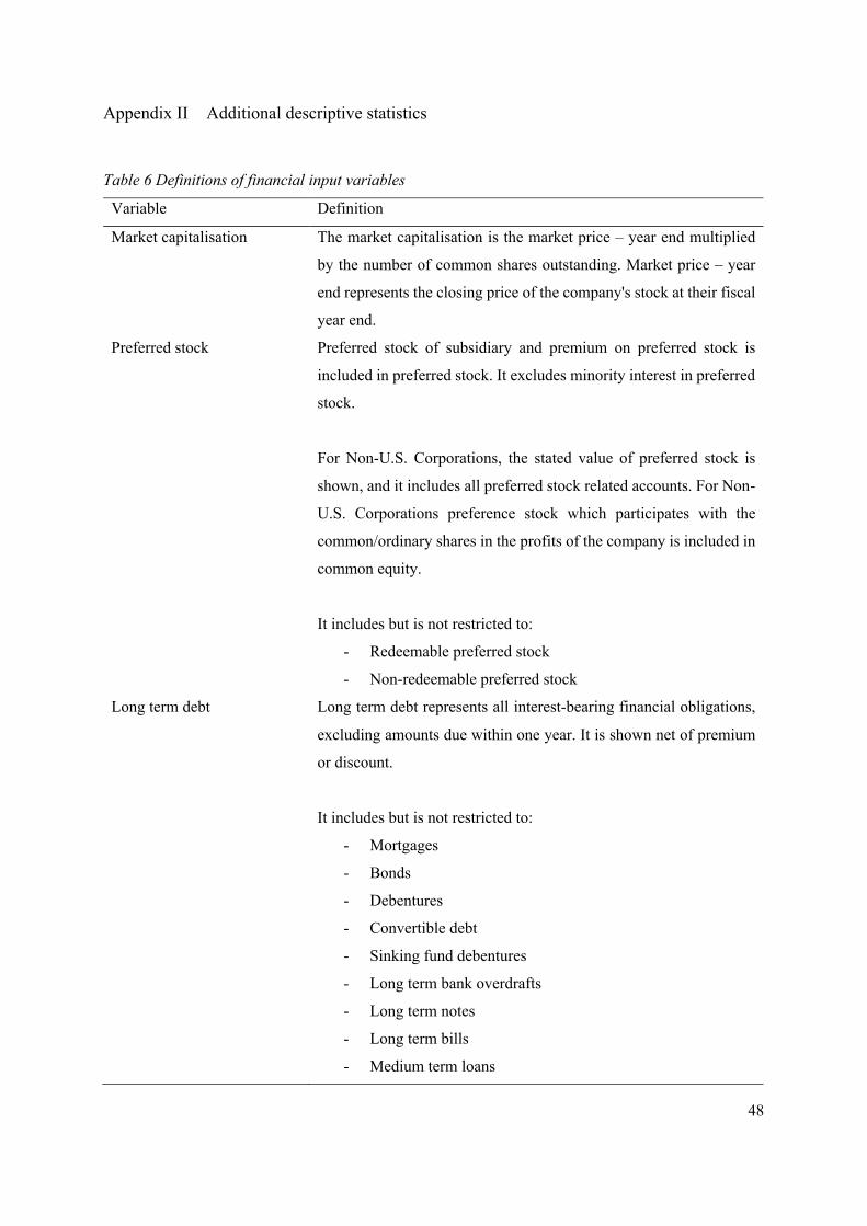
48
Appendix II Additional descriptive statistics
Table 6 Definitions of financial input variables
Variable Definition
Market capitalisation The market capitalisation is the market price – year end multiplied
by the number of common shares outstanding. Market price – year
end represents the closing price of the company's stock at their fiscal
year end.
Preferred stock Preferred stock of subsidiary and premium on preferred stock is
included in preferred stock. It excludes minority interest in preferred
stock.
For Non-U.S. Corporations, the stated value of preferred stock is
shown, and it includes all preferred stock related accounts. For Non-
U.S. Corporations preference stock which participates with the
common/ordinary shares in the profits of the company is included in
common equity.
It includes but is not restricted to:
- Redeemable preferred stock
- Non-redeemable preferred stock
Long term debt Long term debt represents all interest-bearing financial obligations,
excluding amounts due within one year. It is shown net of premium
or discount.
It includes but is not restricted to:
- Mortgages
- Bonds
- Debentures
- Convertible debt
- Sinking fund debentures
- Long term bank overdrafts
- Long term notes
- Long term bills
- Medium term loans
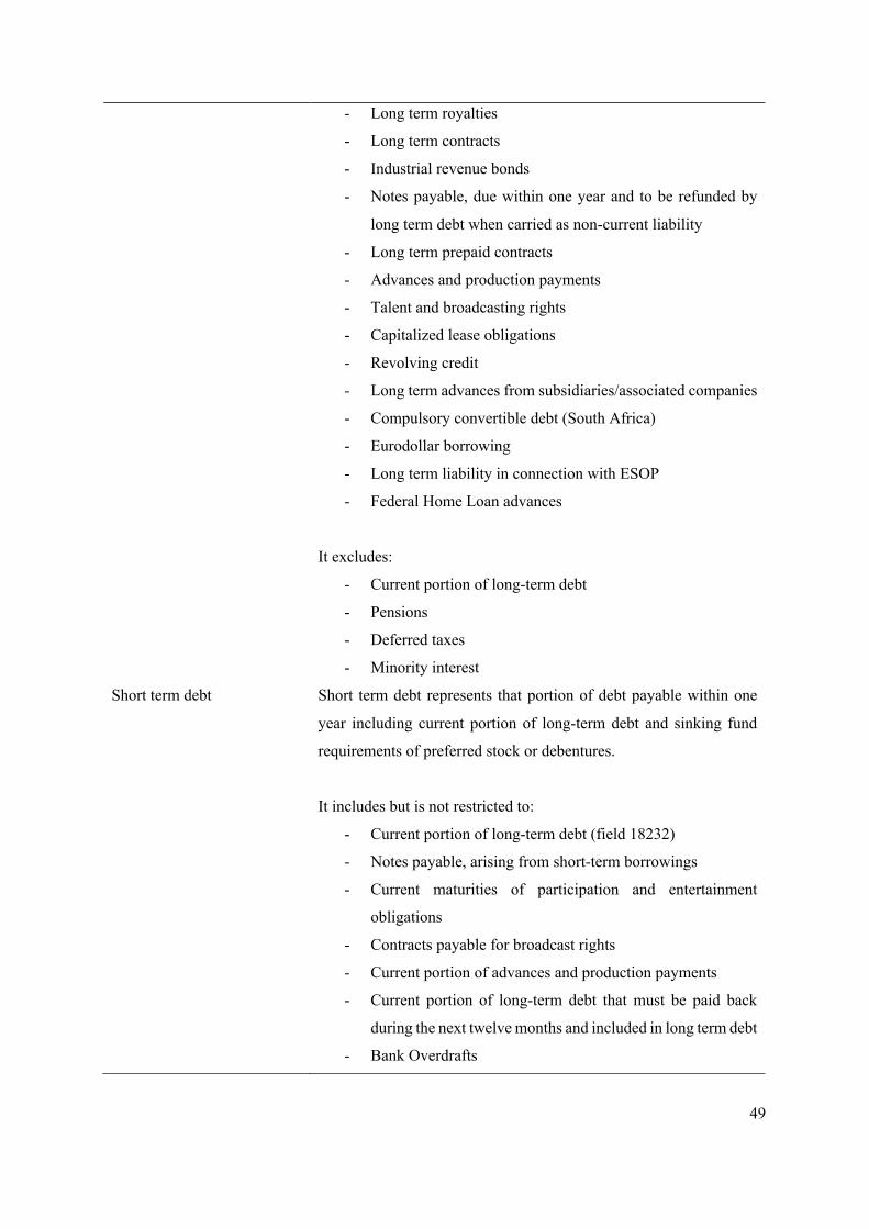
49
- Long term royalties
- Long term contracts
- Industrial revenue bonds
- Notes payable, due within one year and to be refunded by
long term debt when carried as non-current liability
- Long term prepaid contracts
- Advances and production payments
- Talent and broadcasting rights
- Capitalized lease obligations
- Revolving credit
- Long term advances from subsidiaries/associated companies
- Compulsory convertible debt (South Africa)
- Eurodollar borrowing
- Long term liability in connection with ESOP
- Federal Home Loan advances
It excludes:
- Current portion of long-term debt
- Pensions
- Deferred taxes
- Minority interest
Short term debt Short term debt represents that portion of debt payable within one
year including current portion of long-term debt and sinking fund
requirements of preferred stock or debentures.
It includes but is not restricted to:
- Current portion of long-term debt (field 18232)
- Notes payable, arising from short-term borrowings
- Current maturities of participation and entertainment
obligations
- Contracts payable for broadcast rights
- Current portion of advances and production payments
- Current portion of long-term debt that must be paid back
during the next twelve months and included in long term debt
- Bank Overdrafts
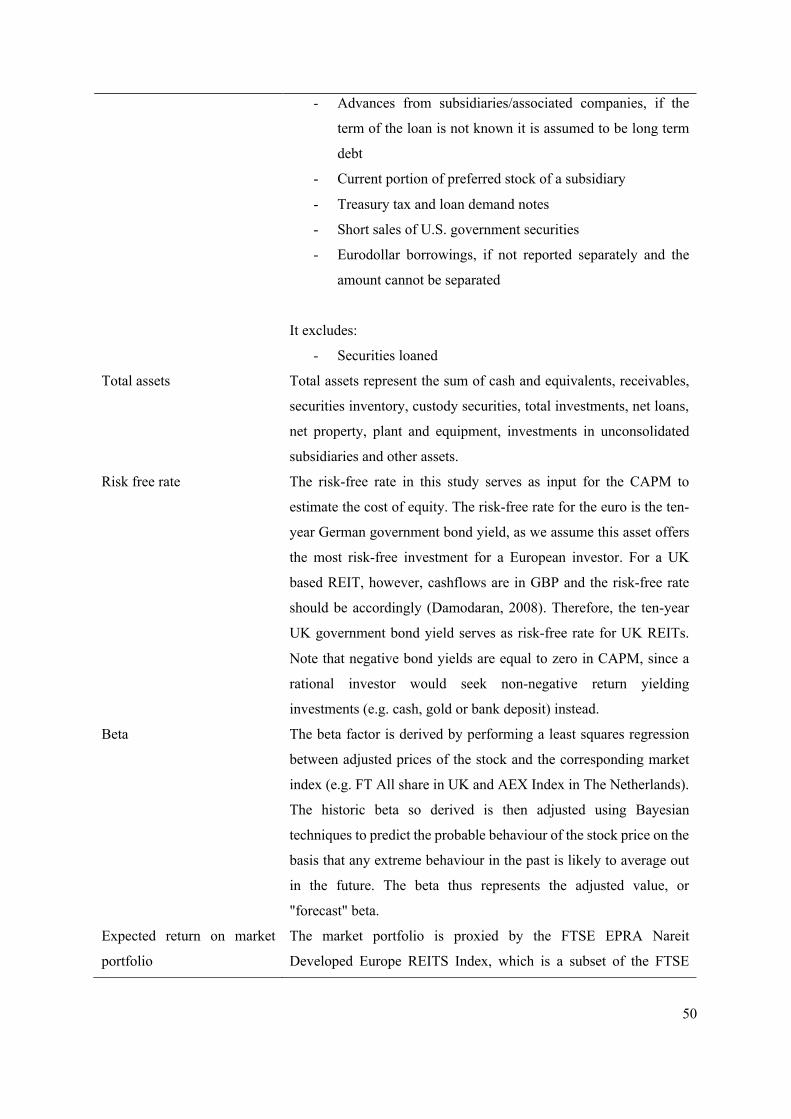
50
- Advances from subsidiaries/associated companies, if the
term of the loan is not known it is assumed to be long term
debt
- Current portion of preferred stock of a subsidiary
- Treasury tax and loan demand notes
- Short sales of U.S. government securities
- Eurodollar borrowings, if not reported separately and the
amount cannot be separated
It excludes:
- Securities loaned
Total assets Total assets represent the sum of cash and equivalents, receivables,
securities inventory, custody securities, total investments, net loans,
net property, plant and equipment, investments in unconsolidated
subsidiaries and other assets.
Risk free rate The risk-free rate in this study serves as input for the CAPM to
estimate the cost of equity. The risk-free rate for the euro is the ten-
year German government bond yield, as we assume this asset offers
the most risk-free investment for a European investor. For a UK
based REIT, however, cashflows are in GBP and the risk-free rate
should be accordingly (Damodaran, 2008). Therefore, the ten-year
UK government bond yield serves as risk-free rate for UK REITs.
Note that negative bond yields are equal to zero in CAPM, since a
rational investor would seek non-negative return yielding
investments (e.g. cash, gold or bank deposit) instead.
Beta The beta factor is derived by performing a least squares regression
between adjusted prices of the stock and the corresponding market
index (e.g. FT All share in UK and AEX Index in The Netherlands).
The historic beta so derived is then adjusted using Bayesian
techniques to predict the probable behaviour of the stock price on the
basis that any extreme behaviour in the past is likely to average out
in the future. The beta thus represents the adjusted value, or
"forecast" beta.
Expected return on market
portfolio
The market portfolio is proxied by the FTSE EPRA Nareit
Developed Europe REITS Index, which is a subset of the FTSE

51
EPRA Nareit Developed Index. The expected return is the year-on-
year performance of the total return (EUR).
Leverage Leverage is the total debt, calculated as the sum of short term debt
and long term debt, divided by the total assets.
Volatility A measure of a stock's average annual price movement to a high and
low from a mean price for each year. For example, a stock's price
volatility of twenty per cent indicates that the stock's annual high and
low price has shown a historical variation of plus twenty per cent to
minus twenty per cent from its annual average price.
Net sales Net sales (or revenues) represent gross sales and other operating
revenue less discounts, returns and allowances.
It includes but is not restricted to:
- Franchise sales when corresponding costs are available and
included in expenses.
- Consulting fees
- Service income
- Royalty income when included in revenues by the company.
- Contracts-in-progress income
- Licensing and franchise fees
- Income derived from equipment lease or rental when
considered part of operating revenue
- Commissions earned (not gross billings) for advertising
companies
- Income from leased departments
It excludes:
- Non-operating income
- Interest income
- Interest capitalized
- Equity in earnings of unconsolidated subsidiaries
- Rental income
- Dividend income
- Foreign exchange adjustment
- Gain on debt retired
- Sale of land or natural resources
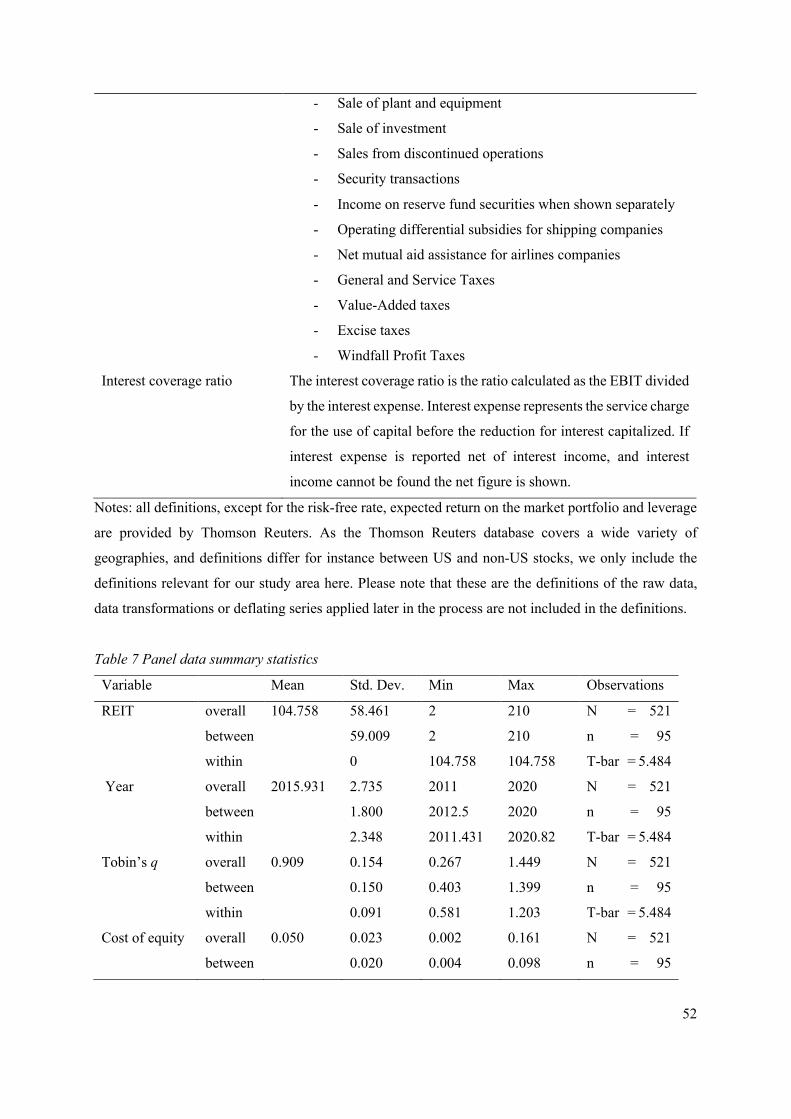
52
- Sale of plant and equipment
- Sale of investment
- Sales from discontinued operations
- Security transactions
- Income on reserve fund securities when shown separately
- Operating differential subsidies for shipping companies
- Net mutual aid assistance for airlines companies
- General and Service Taxes
- Value-Added taxes
- Excise taxes
- Windfall Profit Taxes
Interest coverage ratio The interest coverage ratio is the ratio calculated as the EBIT divided
by the interest expense. Interest expense represents the service charge
for the use of capital before the reduction for interest capitalized. If
interest expense is reported net of interest income, and interest
income cannot be found the net figure is shown.
Notes: all definitions, except for the risk-free rate, expected return on the market portfolio and leverage
are provided by Thomson Reuters. As the Thomson Reuters database covers a wide variety of
geographies, and definitions differ for instance between US and non-US stocks, we only include the
definitions relevant for our study area here. Please note that these are the definitions of the raw data,
data transformations or deflating series applied later in the process are not included in the definitions.
Table 7 Panel data summary statistics
Variable Mean Std. Dev. Min Max Observations
REIT overall
between
within
104.758 58.461
59.009
0
2
2
104.758
210
210
104.758
N = 521
n = 95
T-bar = 5.484
Year overall
between
within
2015.931 2.735
1.800
2.348
2011
2012.5
2011.431
2020
2020
2020.82
N = 521
n = 95
T-bar = 5.484
Tobin’s q overall
between
within
0.909 0.154
0.150
0.091
0.267
0.403
0.581
1.449
1.399
1.203
N = 521
n = 95
T-bar = 5.484
Cost of equity overall
between
0.050
0.023
0.020
0.002
0.004
0.161
0.098
N = 521
n = 95
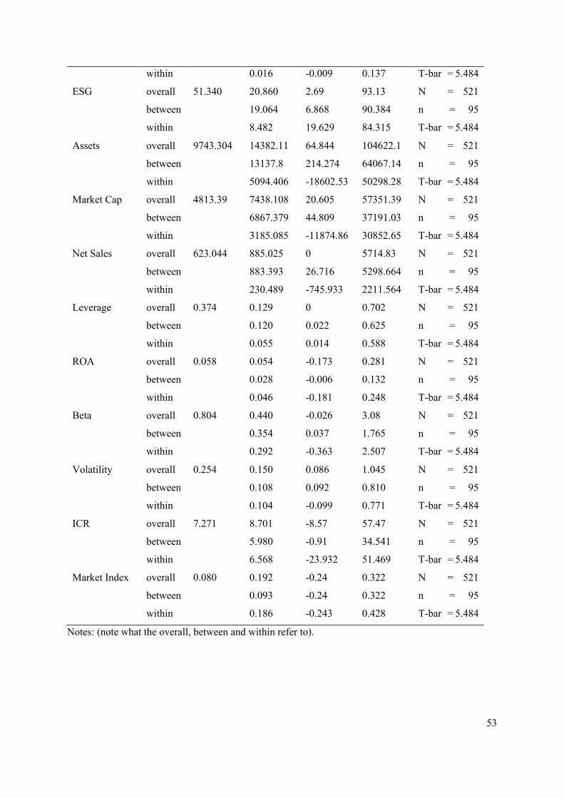
53
within 0.016 -0.009 0.137 T-bar = 5.484
ESG overall
between
within
51.340 20.860
19.064
8.482
2.69
6.868
19.629
93.13
90.384
84.315
N = 521
n = 95
T-bar = 5.484
Assets overall
between
within
9743.304 14382.11
13137.8
5094.406
64.844
214.274
-18602.53
104622.1
64067.14
50298.28
N = 521
n = 95
T-bar = 5.484
Market Cap overall
between
within
4813.39 7438.108
6867.379
3185.085
20.605
44.809
-11874.86
57351.39
37191.03
30852.65
N = 521
n = 95
T-bar = 5.484
Net Sales overall
between
within
623.044 885.025
883.393
230.489
0
26.716
-745.933
5714.83
5298.664
2211.564
N = 521
n = 95
T-bar = 5.484
Leverage overall
between
within
0.374 0.129
0.120
0.055
0
0.022
0.014
0.702
0.625
0.588
N = 521
n = 95
T-bar = 5.484
ROA overall
between
within
0.058 0.054
0.028
0.046
-0.173
-0.006
-0.181
0.281
0.132
0.248
N = 521
n = 95
T-bar = 5.484
Beta overall
between
within
0.804 0.440
0.354
0.292
-0.026
0.037
-0.363
3.08
1.765
2.507
N = 521
n = 95
T-bar = 5.484
Volatility overall
between
within
0.254 0.150
0.108
0.104
0.086
0.092
-0.099
1.045
0.810
0.771
N = 521
n = 95
T-bar = 5.484
ICR overall
between
within
7.271 8.701
5.980
6.568
-8.57
-0.91
-23.932
57.47
34.541
51.469
N = 521
n = 95
T-bar = 5.484
Market Index overall
between
within
0.080 0.192
0.093
0.186
-0.24
-0.24
-0.243
0.322
0.322
0.428
N = 521
n = 95
T-bar = 5.484
Notes: (note what the overall, between and within refer to).
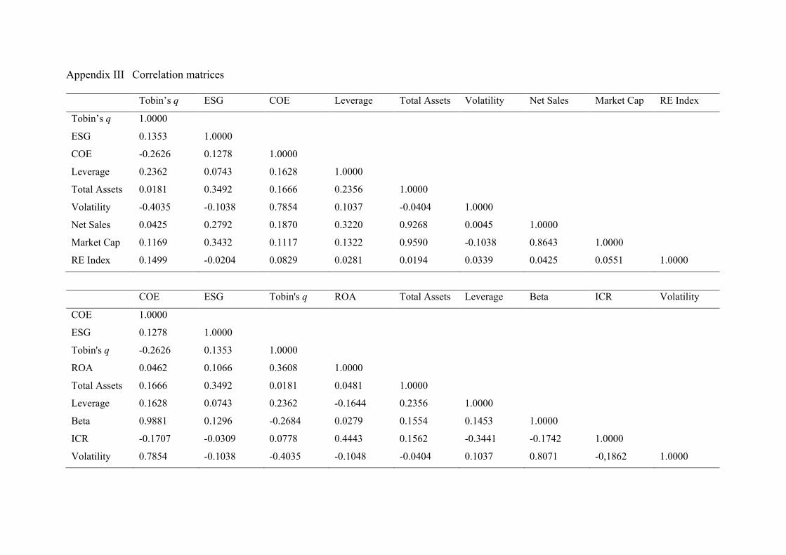
Appendix III Correlation matrices
Tobin’s q ESG COE Leverage Total Assets Volatility Net Sales Market Cap RE Index
Tobin’s q 1.0000
ESG 0.1353 1.0000
COE -0.2626 0.1278 1.0000
Leverage 0.2362 0.0743 0.1628 1.0000
Total Assets 0.0181 0.3492 0.1666 0.2356 1.0000
Volatility -0.4035 -0.1038 0.7854 0.1037 -0.0404 1.0000
Net Sales 0.0425 0.2792 0.1870 0.3220 0.9268 0.0045 1.0000
Market Cap 0.1169 0.3432 0.1117 0.1322 0.9590 -0.1038 0.8643 1.0000
RE Index 0.1499 -0.0204 0.0829 0.0281 0.0194 0.0339 0.0425 0.0551 1.0000
COE ESG Tobin's q ROA Total Assets Leverage Beta ICR Volatility
COE 1.0000
ESG 0.1278 1.0000
Tobin's q -0.2626 0.1353 1.0000
ROA 0.0462 0.1066 0.3608 1.0000
Total Assets 0.1666 0.3492 0.0181 0.0481 1.0000
Leverage 0.1628 0.0743 0.2362 -0.1644 0.2356 1.0000
Beta 0.9881 0.1296 -0.2684 0.0279 0.1554 0.1453 1.0000
ICR -0.1707 -0.0309 0.0778 0.4443 0.1562 -0.3441 -0.1742 1.0000
Volatility 0.7854 -0.1038 -0.4035 -0.1048 -0.0404 0.1037 0.8071 -0,1862 1.0000
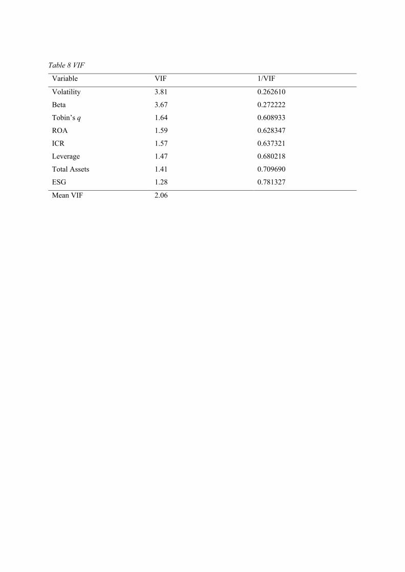
Table 8 VIF
Variable VIF 1/VIF
Volatility 3.81 0.262610
Beta 3.67 0.272222
Tobin’s q 1.64 0.608933
ROA 1.59 0.628347
ICR 1.57 0.637321
Leverage 1.47 0.680218
Total Assets 1.41 0.709690
ESG 1.28 0.781327
Mean VIF 2.06
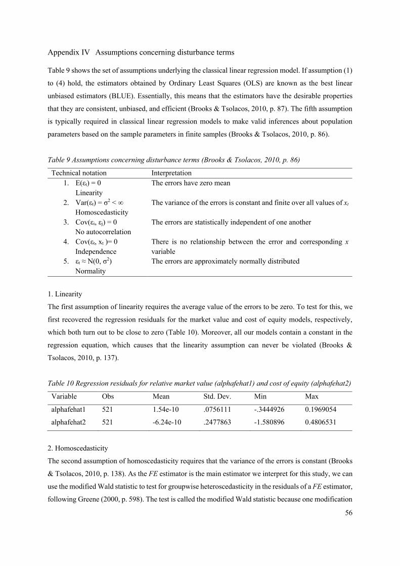
56
Appendix IV Assumptions concerning disturbance terms
Table 9 shows the set of assumptions underlying the classical linear regression model. If assumption (1)
to (4) hold, the estimators obtained by Ordinary Least Squares (OLS) are known as the best linear
unbiased estimators (BLUE). Essentially, this means that the estimators have the desirable properties
that they are consistent, unbiased, and efficient (Brooks & Tsolacos, 2010, p. 87). The fifth assumption
is typically required in classical linear regression models to make valid inferences about population
parameters based on the sample parameters in finite samples (Brooks & Tsolacos, 2010, p. 86).
Table 9 Assumptions concerning disturbance terms (Brooks & Tsolacos, 2010, p. 86)
Technical notation Interpretation 1. E(εt) = 0
Linearity 2. Var(εt) = σ2 < ∞
Homoscedasticity 3. Cov(εi, εj) = 0
No autocorrelation 4. Cov(εt, xt )= 0
Independence 5. εt ≈ N(0, σ2)
Normality
The errors have zero mean The variance of the errors is constant and finite over all values of xt The errors are statistically independent of one another There is no relationship between the error and corresponding x variable The errors are approximately normally distributed
1. Linearity
The first assumption of linearity requires the average value of the errors to be zero. To test for this, we
first recovered the regression residuals for the market value and cost of equity models, respectively,
which both turn out to be close to zero (Table 10). Moreover, all our models contain a constant in the
regression equation, which causes that the linearity assumption can never be violated (Brooks &
Tsolacos, 2010, p. 137).
Table 10 Regression residuals for relative market value (alphafehat1) and cost of equity (alphafehat2)
Variable Obs Mean Std. Dev. Min Max
alphafehat1 521 1.54e-10 .0756111 -.3444926 0.1969054
alphafehat2 521 -6.24e-10 .2477863 -1.580896 0.4806531
2. Homoscedasticity
The second assumption of homoscedasticity requires that the variance of the errors is constant (Brooks
& Tsolacos, 2010, p. 138). As the FE estimator is the main estimator we interpret for this study, we can
use the modified Wald statistic to test for groupwise heteroscedasticity in the residuals of a FE estimator,
following Greene (2000, p. 598). The test is called the modified Wald statistic because one modification

57
has been applied to allow for unbalanced panels, as the one we have at hand. The modified Wald statistic
tests the hypothesis that sigma^2(i)==sigma for i=1,N_g, where N_g is the number of cross-sectional
units. The results of the modified Wald statistic in Table 11 and Table 12 are significant for the market
value and cost of equity models, respectively, rejecting the null hypothesis of homoscedasticity.
Moreover, for small samples and panels with ‘large N, small T’, simulations have shown that its power
is low, and the test should be used with caution. To control for potential heteroscedasticity, we apply
the cluster robust Huber-White standard errors for all models we estimate. The use of cluster robust
Huber-White standard errors also relates to the third assumption of no autocorrelation we discuss next.
Table 11 Modified Wald test for groupwise heteroscedasticity of the market value model
H0: sigma(i)^2 = sigma^2 for all i
chi2 (95) = 27650.56
Prob>chi2 = 0.0000
Table 12 Modified Wald test for groupwise heteroscedasticity of the cost of equity model
H0: sigma(i)^2 = sigma^2 for all i
chi2 (95) = 4.3e+34
Prob>chi2 = 0.0000
3. No autocorrelation
The third assumption of no autocorrelation requires the errors to be uncorrelated with one another
(Brooks & Tsolacos, 2010, p. 144). A priori, it is likely that our data violates the no autocorrelation
assumption as T>2. In fact, Schmidheiny (2020) argues that one can never be sure about the presence of
serial correlation in such panels and advises to always use cluster robust Huber-White standard errors
(see Woolridge, 2002 for a discussion). However, we test for the presence of autocorrelation formally
using the Wooldridge test for autocorrelation in panel data, which Drukker (2003) presents simulation
evidence for that this test has good size and power properties in reasonable sample sizes. The results of
the Wooldridge tests in Table 13 and Table 14, respectively, are significant, rejecting the null hypotheses
of no autocorrelation for the market value and cost of equity models. Therefore, we control for this by
following the advice of Schidheiny (2020) and apply the cluster robust Huber-White standard errors in
all models we estimate.
Table 13 Wooldridge test for the market value model
Wooldridge test for autocorrelation in panel data
H0: no first order autocorrelation
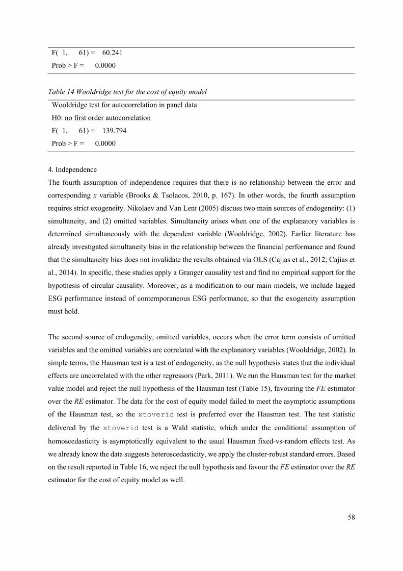
58
F( 1, 61) = 60.241
Prob > F = 0.0000
Table 14 Wooldridge test for the cost of equity model
Wooldridge test for autocorrelation in panel data
H0: no first order autocorrelation
F( 1, 61) = 139.794
Prob > F = 0.0000
4. Independence
The fourth assumption of independence requires that there is no relationship between the error and
corresponding x variable (Brooks & Tsolacos, 2010, p. 167). In other words, the fourth assumption
requires strict exogeneity. Nikolaev and Van Lent (2005) discuss two main sources of endogeneity: (1)
simultaneity, and (2) omitted variables. Simultaneity arises when one of the explanatory variables is
determined simultaneously with the dependent variable (Wooldridge, 2002). Earlier literature has
already investigated simultaneity bias in the relationship between the financial performance and found
that the simultaneity bias does not invalidate the results obtained via OLS (Cajias et al., 2012; Cajias et
al., 2014). In specific, these studies apply a Granger causality test and find no empirical support for the
hypothesis of circular causality. Moreover, as a modification to our main models, we include lagged
ESG performance instead of contemporaneous ESG performance, so that the exogeneity assumption
must hold.
The second source of endogeneity, omitted variables, occurs when the error term consists of omitted
variables and the omitted variables are correlated with the explanatory variables (Wooldridge, 2002). In
simple terms, the Hausman test is a test of endogeneity, as the null hypothesis states that the individual
effects are uncorrelated with the other regressors (Park, 2011). We run the Hausman test for the market
value model and reject the null hypothesis of the Hausman test (Table 15), favouring the FE estimator
over the RE estimator. The data for the cost of equity model failed to meet the asymptotic assumptions
of the Hausman test, so the xtoverid test is preferred over the Hausman test. The test statistic
delivered by the xtoverid test is a Wald statistic, which under the conditional assumption of
homoscedasticity is asymptotically equivalent to the usual Hausman fixed-vs-random effects test. As
we already know the data suggests heteroscedasticity, we apply the cluster-robust standard errors. Based
on the result reported in Table 16, we reject the null hypothesis and favour the FE estimator over the RE
estimator for the cost of equity model as well.
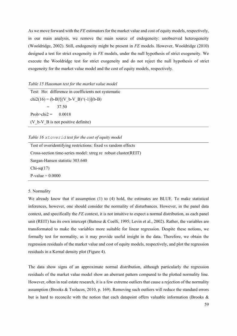
59
As we move forward with the FE estimators for the market value and cost of equity models, respectively,
in our main analysis, we remove the main source of endogeneity: unobserved heterogeneity
(Wooldridge, 2002). Still, endogeneity might be present in FE models. However, Wooldridge (2010)
designed a test for strict exogeneity in FE models, under the null hypothesis of strict exogeneity. We
execute the Wooldridge test for strict exogeneity and do not reject the null hypothesis of strict
exogeneity for the market value model and the cost of equity models, respectively.
Table 15 Hausman test for the market value model
Test: Ho: difference in coefficients not systematic
chi2(16) = (b-B)'[(V_b-V_B)^(-1)](b-B)
= 37.50
Prob>chi2 = 0.0018
(V_b-V_B is not positive definite)
Table 16 xtoverid test for the cost of equity model
Test of overidentifying restrictions: fixed vs random effects
Cross-section time-series model: xtreg re robust cluster(REIT)
Sargan-Hansen statistic 303.640
Chi-sq(17)
P-value = 0.0000
5. Normality
We already know that if assumption (1) to (4) hold, the estimates are BLUE. To make statistical
inferences, however, one should consider the normality of disturbances. However, in the panel data
context, and specifically the FE context, it is not intuitive to expect a normal distribution, as each panel
unit (REIT) has its own intercept (Battese & Coelli, 1995; Levin et al., 2002). Rather, the variables are
transformated to make the variables more suitable for linear regression. Despite these notions, we
formally test for normality, as it may provide useful insight in the data. Therefore, we obtain the
regression residuals of the market value and cost of equity models, respectively, and plot the regression
residuals in a Kernal density plot (Figure 4).
The data show signs of an approximate normal distribution, although particularly the regression
residuals of the market value model show an aberrant pattern compared to the plotted normality line.
However, often in real estate research, it is a few extreme outliers that cause a rejection of the normality
assumption (Brooks & Tsolacos, 2010, p. 169). Removing such outliers will reduce the standard errors
but is hard to reconcile with the notion that each datapoint offers valuable information (Brooks &
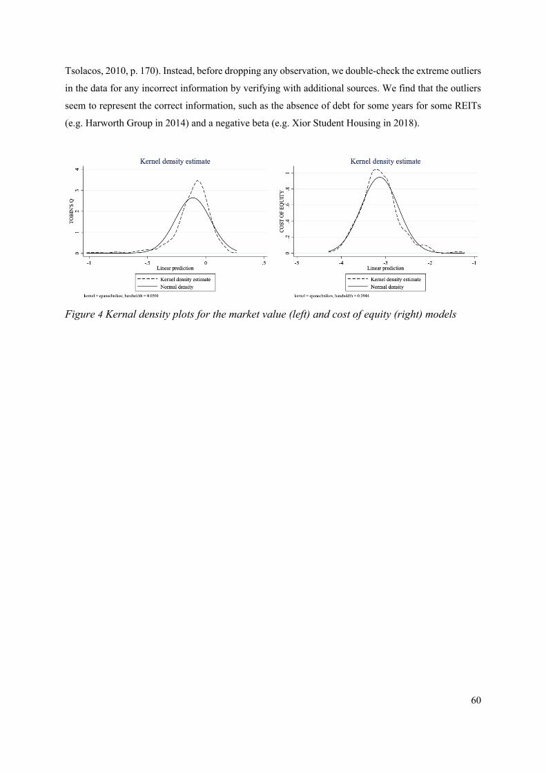
60
Tsolacos, 2010, p. 170). Instead, before dropping any observation, we double-check the extreme outliers
in the data for any incorrect information by verifying with additional sources. We find that the outliers
seem to represent the correct information, such as the absence of debt for some years for some REITs
(e.g. Harworth Group in 2014) and a negative beta (e.g. Xior Student Housing in 2018).
Figure 4 Kernal density plots for the market value (left) and cost of equity (right) models
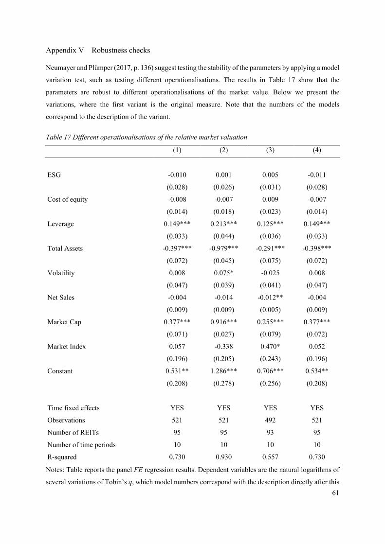
61
Appendix V Robustness checks
Neumayer and Plümper (2017, p. 136) suggest testing the stability of the parameters by applying a model
variation test, such as testing different operationalisations. The results in Table 17 show that the
parameters are robust to different operationalisations of the market value. Below we present the
variations, where the first variant is the original measure. Note that the numbers of the models
correspond to the description of the variant.
Table 17 Different operationalisations of the relative market valuation
(1) (2) (3) (4)
ESG -0.010 0.001 0.005 -0.011
(0.028) (0.026) (0.031) (0.028)
Cost of equity -0.008 -0.007 0.009 -0.007
(0.014) (0.018) (0.023) (0.014)
Leverage 0.149*** 0.213*** 0.125*** 0.149***
(0.033) (0.044) (0.036) (0.033)
Total Assets -0.397*** -0.979*** -0.291*** -0.398***
(0.072) (0.045) (0.075) (0.072)
Volatility 0.008 0.075* -0.025 0.008
(0.047) (0.039) (0.041) (0.047)
Net Sales -0.004 -0.014 -0.012** -0.004
(0.009) (0.009) (0.005) (0.009)
Market Cap 0.377*** 0.916*** 0.255*** 0.377***
(0.071) (0.027) (0.079) (0.072)
Market Index 0.057 -0.338 0.470* 0.052
(0.196) (0.205) (0.243) (0.196)
Constant 0.531** 1.286*** 0.706*** 0.534**
(0.208) (0.278) (0.256) (0.208)
Time fixed effects YES YES YES YES
Observations 521 521 492 521
Number of REITs 95 95 93 95
Number of time periods 10 10 10 10
R-squared 0.730 0.930 0.557 0.730
Notes: Table reports the panel FE regression results. Dependent variables are the natural logarithms of
several variations of Tobin’s q, which model numbers correspond with the description directly after this
62
table. Cluster-robust Huber-White standard errors (clustered by REIT) in parentheses. Significance at
*** p<0.01, ** p<0.05 and * p<0.1, respectively.
(1) Tobin’s q The first variation of Tobin’s q is the main measure discussed in the third chapter, and has been widely
used in studies with a similar research aim (Cajias et al., 2014; Han, 2006; Konar & Cohen, 2001). We
operationalise the Tobin’s q following Perfect and Wiles (1994):
!" = $%& +$%( + *!+ + ,!+!- (5)
Where Tq denotes the Tobin’s q; MVC denotes the market value of common stocks; MVP the market
value of preferred securities; LTD the book value of long-term debt; STD the book value of short-term
debt, and; TA the book value of total assets.
(2) Tobin’s q The second variation is defined by the Network for Business Sustainability (Turner, 2013), and transfers
the debt from the nominator to the denominator. The rationale to do so lies in the fact that the
replacement cost of assets should reflect the firm’s net assets. Therefore, we specify the second Tobin’s
q variation as follows:
!" = $%& +$%(!- + *!+ + ,!+ (6)
Where Tq denotes the Tobin’s q; MVC denotes the market value of common stocks; MVP the market
value of preferred securities; LTD the book value of long-term debt; STD the book value of short-term
debt, and; TA the book value of total assets.
(3) Tobin’s q The third variation is used in several governance and ESG disclosure papers which use Tobin’s q to
proxy firm performance (Bauer et al. 2010; Fatemi et al., 2018; Servaes & Tamayo, 2013). The total
value of the firm is determined by the market cap and total assets, from which the book value of equity
and deferred taxes are subtracted, leading to:
!" = $%& + !- − /%0 − +01!-2!- (7)
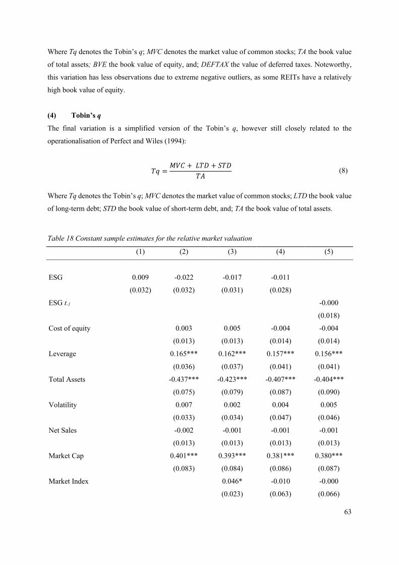
63
Where Tq denotes the Tobin’s q; MVC denotes the market value of common stocks; TA the book value
of total assets; BVE the book value of equity, and; DEFTAX the value of deferred taxes. Noteworthy,
this variation has less observations due to extreme negative outliers, as some REITs have a relatively
high book value of equity.
(4) Tobin’s q
The final variation is a simplified version of the Tobin’s q, however still closely related to the
operationalisation of Perfect and Wiles (1994):
!" = $%& + *!+ + ,!+!- (8)
Where Tq denotes the Tobin’s q; MVC denotes the market value of common stocks; LTD the book value
of long-term debt; STD the book value of short-term debt, and; TA the book value of total assets.
Table 18 Constant sample estimates for the relative market valuation
(1) (2) (3) (4) (5)
ESG 0.009 -0.022 -0.017 -0.011
(0.032) (0.032) (0.031) (0.028)
ESG t-1 -0.000
(0.018)
Cost of equity 0.003 0.005 -0.004 -0.004
(0.013) (0.013) (0.014) (0.014)
Leverage 0.165*** 0.162*** 0.157*** 0.156***
(0.036) (0.037) (0.041) (0.041)
Total Assets -0.437*** -0.423*** -0.407*** -0.404***
(0.075) (0.079) (0.087) (0.090)
Volatility 0.007 0.002 0.004 0.005
(0.033) (0.034) (0.047) (0.046)
Net Sales -0.002 -0.001 -0.001 -0.001
(0.013) (0.013) (0.013) (0.013)
Market Cap 0.401*** 0.393*** 0.381*** 0.380***
(0.083) (0.084) (0.086) (0.087)
Market Index 0.046* -0.010 -0.000
(0.023) (0.063) (0.066)
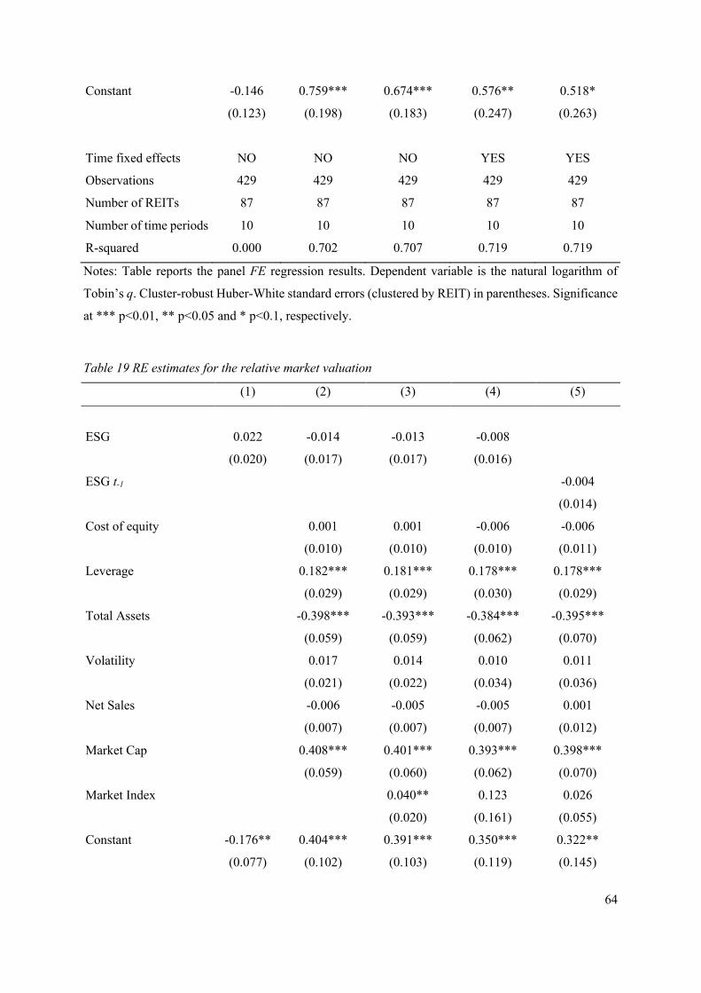
64
Constant -0.146 0.759*** 0.674*** 0.576** 0.518*
(0.123) (0.198) (0.183) (0.247) (0.263)
Time fixed effects NO NO NO YES YES
Observations 429 429 429 429 429
Number of REITs 87 87 87 87 87
Number of time periods 10 10 10 10 10
R-squared 0.000 0.702 0.707 0.719 0.719
Notes: Table reports the panel FE regression results. Dependent variable is the natural logarithm of
Tobin’s q. Cluster-robust Huber-White standard errors (clustered by REIT) in parentheses. Significance
at *** p<0.01, ** p<0.05 and * p<0.1, respectively.
Table 19 RE estimates for the relative market valuation
(1) (2) (3) (4) (5)
ESG 0.022 -0.014 -0.013 -0.008
(0.020) (0.017) (0.017) (0.016)
ESG t-1 -0.004
(0.014)
Cost of equity 0.001 0.001 -0.006 -0.006
(0.010) (0.010) (0.010) (0.011)
Leverage 0.182*** 0.181*** 0.178*** 0.178***
(0.029) (0.029) (0.030) (0.029)
Total Assets -0.398*** -0.393*** -0.384*** -0.395***
(0.059) (0.059) (0.062) (0.070)
Volatility 0.017 0.014 0.010 0.011
(0.021) (0.022) (0.034) (0.036)
Net Sales -0.006 -0.005 -0.005 0.001
(0.007) (0.007) (0.007) (0.012)
Market Cap 0.408*** 0.401*** 0.393*** 0.398***
(0.059) (0.060) (0.062) (0.070)
Market Index 0.040** 0.123 0.026
(0.020) (0.161) (0.055)
Constant -0.176** 0.404*** 0.391*** 0.350*** 0.322**
(0.077) (0.102) (0.103) (0.119) (0.145)

65
Time fixed effects NO NO NO YES YES
Observations 521 521 521 521 429
Number of REITs 95 95 95 95 87
Number of time periods 10 10 10 10 10
Notes: Table reports the panel RE regression results. Dependent variable is the natural logarithm of
Tobin’s q. Cluster-robust Huber-White standard errors (clustered by REIT) in parentheses. Significance
at *** p<0.01, ** p<0.05 and * p<0.1, respectively.
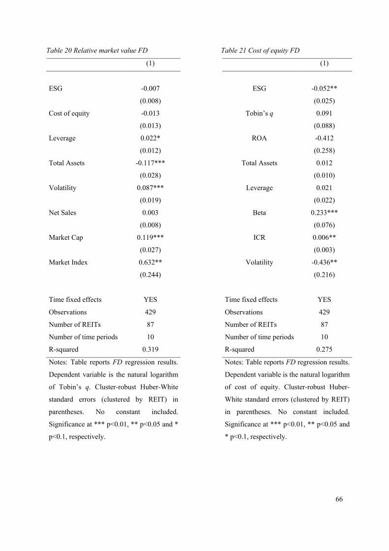
66
Table 20 Relative market value FD Table 21 Cost of equity FD
(1) (1)
ESG -0.007 ESG -0.052**
(0.008) (0.025)
Cost of equity -0.013 Tobin’s q 0.091
(0.013) (0.088)
Leverage 0.022* ROA -0.412
(0.012) (0.258)
Total Assets -0.117*** Total Assets 0.012
(0.028) (0.010)
Volatility 0.087*** Leverage 0.021
(0.019) (0.022)
Net Sales 0.003 Beta 0.233***
(0.008) (0.076)
Market Cap 0.119*** ICR 0.006**
(0.027) (0.003)
Market Index 0.632** Volatility -0.436**
(0.244) (0.216)
Time fixed effects YES Time fixed effects YES
Observations 429 Observations 429
Number of REITs 87 Number of REITs 87
Number of time periods 10 Number of time periods 10
R-squared 0.319 R-squared 0.275
Notes: Table reports FD regression results.
Dependent variable is the natural logarithm
of Tobin’s q. Cluster-robust Huber-White
standard errors (clustered by REIT) in
parentheses. No constant included.
Significance at *** p<0.01, ** p<0.05 and *
p<0.1, respectively.
Notes: Table reports FD regression results.
Dependent variable is the natural logarithm
of cost of equity. Cluster-robust Huber-
White standard errors (clustered by REIT)
in parentheses. No constant included.
Significance at *** p<0.01, ** p<0.05 and
* p<0.1, respectively.
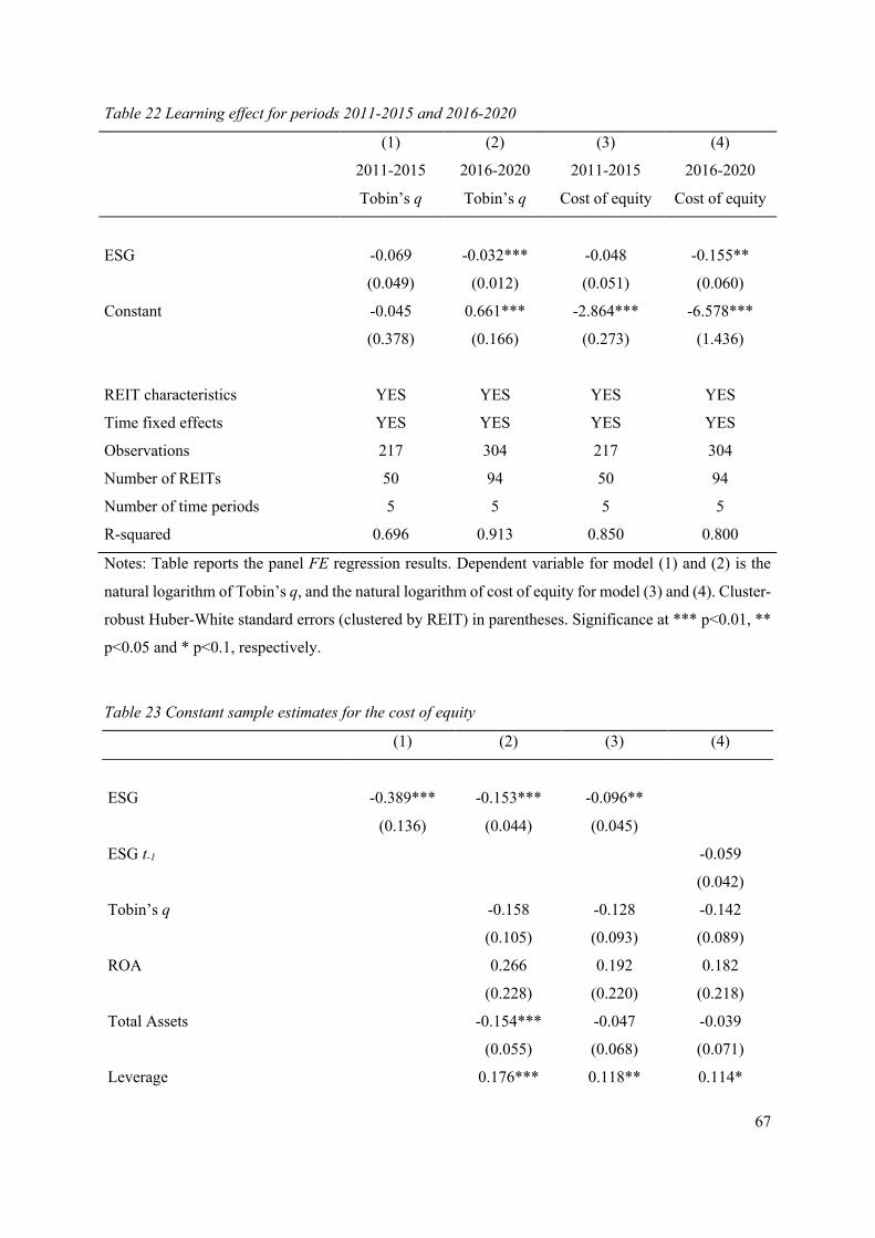
67
Table 22 Learning effect for periods 2011-2015 and 2016-2020
(1) (2) (3) (4)
2011-2015
Tobin’s q
2016-2020
Tobin’s q
2011-2015
Cost of equity
2016-2020
Cost of equity
ESG -0.069 -0.032*** -0.048 -0.155**
(0.049) (0.012) (0.051) (0.060)
Constant -0.045 0.661*** -2.864*** -6.578***
(0.378) (0.166) (0.273) (1.436)
REIT characteristics YES YES YES YES
Time fixed effects YES YES YES YES
Observations 217 304 217 304
Number of REITs 50 94 50 94
Number of time periods 5 5 5 5
R-squared 0.696 0.913 0.850 0.800
Notes: Table reports the panel FE regression results. Dependent variable for model (1) and (2) is the
natural logarithm of Tobin’s q, and the natural logarithm of cost of equity for model (3) and (4). Cluster-
robust Huber-White standard errors (clustered by REIT) in parentheses. Significance at *** p<0.01, **
p<0.05 and * p<0.1, respectively.
Table 23 Constant sample estimates for the cost of equity
(1) (2) (3) (4)
ESG -0.389*** -0.153*** -0.096**
(0.136) (0.044) (0.045)
ESG t-1 -0.059
(0.042)
Tobin’s q -0.158 -0.128 -0.142
(0.105) (0.093) (0.089)
ROA 0.266 0.192 0.182
(0.228) (0.220) (0.218)
Total Assets -0.154*** -0.047 -0.039
(0.055) (0.068) (0.071)
Leverage 0.176*** 0.118** 0.114*
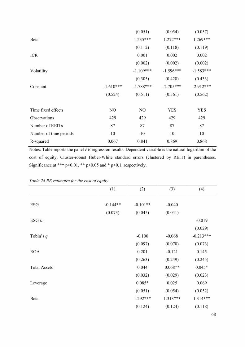
68
(0.051) (0.054) (0.057)
Beta 1.235*** 1.272*** 1.269***
(0.112) (0.118) (0.119)
ICR 0.001 0.002 0.002
(0.002) (0.002) (0.002)
Volatility -1.109*** -1.596*** -1.583***
(0.305) (0.428) (0.433)
Constant -1.610*** -1.788*** -2.705*** -2.912***
(0.524) (0.511) (0.561) (0.562)
Time fixed effects NO NO YES YES
Observations 429 429 429 429
Number of REITs 87 87 87 87
Number of time periods 10 10 10 10
R-squared 0.067 0.841 0.869 0.868
Notes: Table reports the panel FE regression results. Dependent variable is the natural logarithm of the
cost of equity. Cluster-robust Huber-White standard errors (clustered by REIT) in parentheses.
Significance at *** p<0.01, ** p<0.05 and * p<0.1, respectively.
Table 24 RE estimates for the cost of equity
(1) (2) (3) (4)
ESG -0.144** -0.101** -0.040
(0.073) (0.045) (0.041)
ESG t-1 -0.019
(0.029)
Tobin’s q -0.100 -0.068 -0.213***
(0.097) (0.078) (0.073)
ROA 0.201 -0.121 0.145
(0.263) (0.249) (0.245)
Total Assets 0.044 0.068** 0.045*
(0.032) (0.029) (0.023)
Leverage 0.085* 0.025 0.069
(0.051) (0.054) (0.052)
Beta 1.292*** 1.313*** 1.314***
(0.124) (0.124) (0.118)
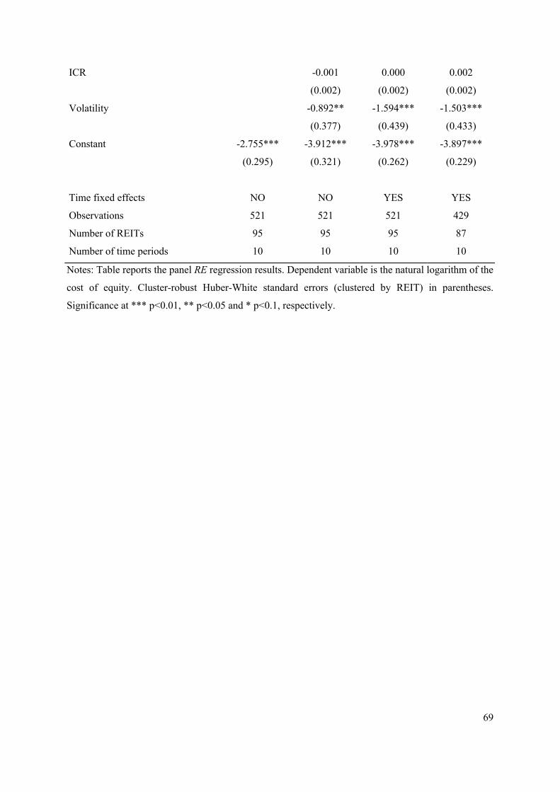
69
ICR -0.001 0.000 0.002
(0.002) (0.002) (0.002)
Volatility -0.892** -1.594*** -1.503***
(0.377) (0.439) (0.433)
Constant -2.755*** -3.912*** -3.978*** -3.897***
(0.295) (0.321) (0.262) (0.229)
Time fixed effects NO NO YES YES
Observations 521 521 521 429
Number of REITs 95 95 95 87
Number of time periods 10 10 10 10
Notes: Table reports the panel RE regression results. Dependent variable is the natural logarithm of the
cost of equity. Cluster-robust Huber-White standard errors (clustered by REIT) in parentheses.
Significance at *** p<0.01, ** p<0.05 and * p<0.1, respectively.
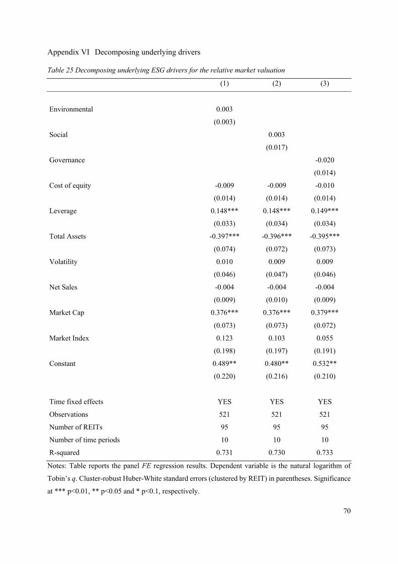
70
Appendix VI Decomposing underlying drivers
Table 25 Decomposing underlying ESG drivers for the relative market valuation
(1) (2) (3)
Environmental 0.003
(0.003)
Social 0.003
(0.017)
Governance -0.020
(0.014)
Cost of equity -0.009 -0.009 -0.010
(0.014) (0.014) (0.014)
Leverage 0.148*** 0.148*** 0.149***
(0.033) (0.034) (0.034)
Total Assets -0.397*** -0.396*** -0.395***
(0.074) (0.072) (0.073)
Volatility 0.010 0.009 0.009
(0.046) (0.047) (0.046)
Net Sales -0.004 -0.004 -0.004
(0.009) (0.010) (0.009)
Market Cap 0.376*** 0.376*** 0.379***
(0.073) (0.073) (0.072)
Market Index 0.123 0.103 0.055
(0.198) (0.197) (0.191)
Constant 0.489** 0.480** 0.532**
(0.220) (0.216) (0.210)
Time fixed effects YES YES YES
Observations 521 521 521
Number of REITs 95 95 95
Number of time periods 10 10 10
R-squared 0.731 0.730 0.733
Notes: Table reports the panel FE regression results. Dependent variable is the natural logarithm of
Tobin’s q. Cluster-robust Huber-White standard errors (clustered by REIT) in parentheses. Significance
at *** p<0.01, ** p<0.05 and * p<0.1, respectively.
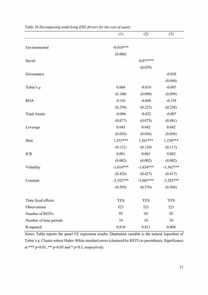
71
Table 26 Decomposing underlying ESG drivers for the cost of equity
(1) (2) (3)
Environmental -0.018***
(0.006)
Social -0.077***
(0.029)
Governance -0.028
(0.040)
Tobin’s q 0.004 -0.010 -0.007
(0.100) (0.098) (0.099)
ROA -0.141 -0.048 -0.139
(0.239) (0.225) (0.238)
Total Assets -0.006 -0.022 -0.007
(0.077) (0.075) (0.081)
Leverage 0.045 0.042 0.042
(0.056) (0.056) (0.056)
Beta 1.253*** 1.261*** 1.230***
(0.121) (0.120) (0.117)
ICR 0.001 0.001 0.002
(0.002) (0.002) (0.002)
Volatility -1.616*** -1.634*** -1.562***
(0.426) (0.427) (0.417)
Constant -3.352*** -3.003*** -3.292***
(0.595) (0.570) (0.560)
Time fixed effects YES YES YES
Observations 521 521 521
Number of REITs 95 95 95
Number of time periods 10 10 10
R-squared 0.810 0.811 0.808
Notes: Table reports the panel FE regression results. Dependent variable is the natural logarithm of
Tobin’s q. Cluster-robust Huber-White standard errors (clustered by REIT) in parentheses. Significance
at *** p<0.01, ** p<0.05 and * p<0.1, respectively.