ESD.70J / 1.145J Engineering Economy Module · Fall 2009 For information ... “Data Analysis” package, but it won’t refresh. ... and decision-makers! ESD.70J Engineering Economy

MIT OpenCourseWarehttp://ocw.mit.edu

ESD.70J / 1.145J Engineering Economy Module Fall 2009

For information about citing these materials or our Terms of Use, visit: http://ocw.mit.edu/terms.

http://ocw.mit.edu/terms

http://ocw.mit.edu

ESD.70J Engineering Economy Module - Session 2 1

ESD.70J Engineering Economy

Fall 2009Session Two

Michel-Alexandre CardinProf. Richard de Neufville


Session two – Simulation

• Objectives: – Generate random numbers– Get familiar with Monte Carlo simulation– Set up simulation using Data Table– Generate statistics for simulation – Draw histogram and cumulative distribution

function (CDF)• Also called “Target curve”


Questions for “Big vs. Small”From the base case spreadsheet, we’ve calculated

NPVsHowever, we assumed deterministic demand

forecasts for years 1, 2, and 3. This assumption is over-simplifying since actual demand will vary

⇒ Since life in uncertain, we want to simulate a range of possible NPV outcomes, the Min, Max, distributions, and the expected NPV values!


Set up random generator

Open ESD70session2-1.xls


Excel’s RAND() function• Returns random number greater than or

equal to 0 and less than 1, sampled from a uniform distribution

• To generate a random real number between a and b, use: =RAND()*(b-a)+a

• In tab “RAND”, the formula in cell C3: “=Entries!C9*((1-Entries!C25)+2*Entries!C25*RAND())”– Returns a uniformly distributed random demand for year 1 centered

around 300, which may differ by plus or minus 50%

• Same logic applies for cell C4 and C5


Random number generatorFollow the instructions, step by step

1. Go to tab “RAND”2. Type “=Entries!C9*((1-

Entries!C25)+2*Entries!C25*RAND())” in cell C33. Type “=Entries!C10*((1-

Entries!C25)+2*Entries!C25*RAND())” in cell D34. Type “=Entries!C11*((1-

Entries!C25)+2*Entries!C25*RAND())” in cell E35. Press “F9” several times to see what happens


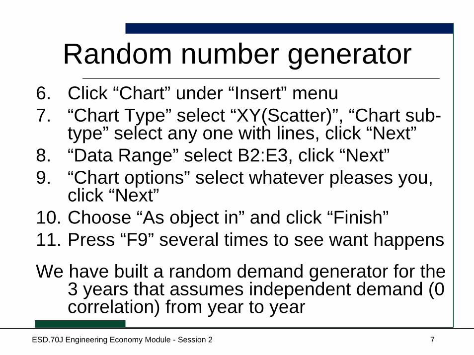
6. Click “Chart” under “Insert” menu7. “Chart Type” select “XY(Scatter)”, “Chart sub-

type” select any one with lines, click “Next”8. “Data Range” select B2:E3, click “Next”9. “Chart options” select whatever pleases you,

click “Next”10. Choose “As object in” and click “Finish”11. Press “F9” several times to see want happens

We have built a random demand generator for the 3 years that assumes independent demand (0 correlation) from year to year

Random number generator


Give it a try!

Check with your neighbors…

Check the solution sheet…

Ask me questions…


How Monte Carlo Simulation works

Calculate two NPVAs corresponding to the two random demand simulations

Demand in Year 1

Demand in Year 2

Demand in Year 3

NPVA

345 678 1001 ?189 579 690 ?

How about generating many sets of random demands, and get the corresponding NPVAs automatically?


Monte Carlo SimulationGenerate many sets of random price for the

three-phase span

Calculate corresponding NPVs

Generate Distribution of NPVs

Statistical Analysis


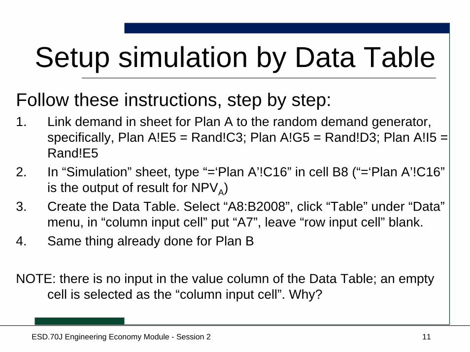
Setup simulation by Data TableFollow these instructions, step by step:1. Link demand in sheet for Plan A to the random demand generator,

specifically, Plan A!E5 = Rand!C3; Plan A!G5 = Rand!D3; Plan A!I5 = Rand!E5

2. In “Simulation” sheet, type “=‘Plan A’!C16” in cell B8 (“=‘Plan A’!C16”is the output of result for NPVA)

3. Create the Data Table. Select “A8:B2008”, click “Table” under “Data”menu, in “column input cell” put “A7”, leave “row input cell” blank.

4. Same thing already done for Plan B

NOTE: there is no input in the value column of the Data Table; an empty cell is selected as the “column input cell”. Why?


Explanation• For the One-Way Data Table, there is no

need to set up the input values in a list, since each row of the Data Table calls RAND() and generates an NPVAprojection

• We have 2,000 rows in the Data Table, so we have simulated 2000 times

• Click “command =” or “F9” to try another simulation run


Excel crashing noteIf your Excel crashes during simulation

runs, input some numbers (0’s or whatever) into the input value column to the left of the data series. Do not leave the area of input values blank in the Data Table

You can hide the dummy values by setting their font value to “white” color


Give it a try!



Ask me questions…


Calculating descriptive statistics

• Useful to know mean, maximum, and minimum values for the simulated results

Follow step by step:1. In Cell D1 type “=AVERAGE(B$9:B$2008)”2. In Cell D2 type “=MAX(B$9:B$2008)”3. In Cell D3 type “=MIN(B$9:B$2008)”


Give it a try!



Ask me questions…


Deterministic vs. dynamic results

• From the base case spreadsheet, we learn NPVA is $162.1 million

• What is your result for the expected NPVAand NPVB when considering demand uncertainty?

• Jensen’s inequality and the Flaw of Averages: )]([)]([ xfExEf ≠


Target curve• The target curve is another name for cumulative

distribution function (CDF)

• In our case, a target curve aims at making a representation to managers that– “There is a probability X that NPV will be lower (higher) than a

targeted Y dollars for this project”

• Value At Risk is a common language on Wall Street. It stresses downside risk, though we should also look at CDF for upside potential of a project, or Value At Gain!


Target curve

Follow the instructions, step by step:1. In sheet “Simulation”, set Cell G7 “=$D$3+($D$2-

$D$3)/20*F7”, and drag the formula down to G272. Set Cell H7

“=COUNTIF($B$9:$B$2008,"<="&G7)”, and drag the formula down to H27

3. Set Cell I7 “=H7/2000”, and drag down to cell I274. Same is already done for Plan B


6. Right-click the chart on the right, select “Source Data”

7. Select “Series”, and press “Add”. This adds a new data series to the graph. Call it “NPVA”

8. Select the range =Simulation!$G$7:$G$27 for X values, and the range =Simulation!$I$7:$I$27 for Y values. Click “OK”

9. Right-click the curve and change “Weight” to 310. Hit “command =” or “F9” and watch the target curve

move !

Target curve


Explanation• We set up 20 data buckets and count how

many data points fall into each interval• “=COUNTIF()” function counts the number of

cells within a range that meet the criteria• The Excel file demonstrates how you can:

– Add NPVA and NPVB means as vertical lines– Add histograms for two NPV distributions using the

information created earlier• Can also use the Histogram analysis tool in

“Data Analysis” package, but it won’t refresh


Values At Risk and Gain• Use your cursor on the graph to find different

Values At Risk and Values At Gain• Alternatively, use the percentile function

– In cell N5, type 10%– In cell R5, type “=PERCENTILE(B9:B2008,N5)”

• What does this tell you?• That’s interesting information for managers

and decision-makers!


Question

• Why are high NPV values more cut off for Plan B on the target curve and histogram than for Plan A?– A matter of constraints…


Give it a try!



Ask me questions…


Summary• Random number generation is fairly

straight forward in Excel• At least two ways to run Monte Carlo

simulation:– Direct RAND() calls - too long…– Using Data Table - the way to go!

• Descriptive statistics from simulations– Mean, Max, Min, target curve


Next class…• Today’s session modeled demand

uncertainty based on a uniformly distributed random variable

• This is not a particularly realistic model, though it is simple and sufficient for today’s purposes

• Next session explores alternative probability distributions from which to sample and stochastic models. STAY TUNED!

Documents

ESD.70J / 1.145J Engineering Economy Module · Fall 2009 For information ... “Data Analysis” package, but it won’t refresh. ... and decision-makers! ESD.70J Engineering Economy