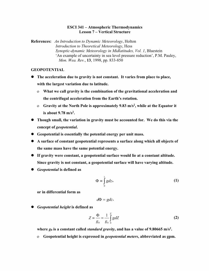
ESCI 341 – Atmospheric Thermodynamics Lesson 7 – Vertical Structure

References: An Introduction to Dynamic Meteorology, Holton

Introduction to Theoretical Meteorology, Hess Synoptic-dynamic Meteorology in Midlatitudes, Vol. 1, Bluestein ‘An example of uncertainty in sea level pressure reduction’, P.M. Pauley,

Mon. Wea. Rev., 13, 1998, pp. 833-850 GEOPOTENTIAL

l The acceleration due to gravity is not constant. It varies from place to place,

with the largest variation due to latitude.

o What we call gravity is the combination of the gravitational acceleration and

the centrifugal acceleration from the Earth’s rotation.

o Gravity at the North Pole is approximately 9.83 m/s2, while at the Equator it

is about 9.78 m/s2.

l Though small, the variation in gravity must be accounted for. We do this via the

concept of geopotential.

l Geopotential is essentially the potential energy per unit mass.

l A surface of constant geopotential represents a surface along which all objects of

the same mass have the same potential energy.

l If gravity were constant, a geopotential surface would lie at a constant altitude.

Since gravity is not constant, a geopotential surface will have varying altitude.

l Geopotential is defined as

, (1)

or in differential form as

.

l Geopotential height is defined as

(2)

where g0 is a constant called standard gravity, and has a value of 9.80665 m/s2.

o Geopotential height is expressed in geopotential meters, abbreviated as gpm.

òºFz

gdz0

gdzd =F

0 0 0

1 Z

Z gdZg gF

º = ò

2

l If the change in gravity with height is ignored, geopotential height and geometric

height are related via

. (3)

o If the local gravity is stronger than standard gravity, then Z > z.

o If the local gravity is weaker than standard gravity, then Z < z.

l Gravity varies from around 9.79 to 9.82 m/s2. Therefore, g/g0 @ 1, and for many

applications we can ignore the difference between geopotential and geometric

height, since Z @ z.

o But, keep in mind that they are different, and at times this difference, though

small, is very important and cannot be neglected.

l Many equations, such as the hydrostatic equation or the hypsometric equation,

can be written either in terms of geometric height or geopotential height. A

convenient rule that applies most of the time is that

o if the formula is written in geopotential height, Z, then g0 is used for gravity.

o if the formula is written in geometric height, z, then g is used for gravity.

o Example: The hydrostatic equation can be written both ways, as shown

below

PRESSURE

l Pressure is force per unit area.

l There are two types of pressure:

o Hydrostatic pressure, which is just due to the weight of the air above you.

o Dynamic pressure, which is due to the motion of the air.

l In meteorology, dynamic pressure is usually very small, and we will assume for

now that atmospheric pressure is solely due to hydrostatic pressure.

l To find how pressure changes with height we start with the hydrostatic equation

zggZ0

=

0gZp

gzp

r

r

-=¶¶

-=¶¶

3

,

and the ideal gas law

.

o Eliminating density from these two equation gives

. (4)

o Integrating vertically from the surface to some height z we get

or

. Pressure variation with height (5)

PRESSURE DECREASE IN AN ISOTHERMAL ATMOSPHERE

l Absolute temperature varies by only 20% or so through the troposphere, so we

can get an idea how pressure changes with height by assuming a constant

temperature (isothermal atmosphere). If this is done, the expression for the

pressure profile becomes

. (6)

l HP is the pressure scale height of the atmosphere, and is a measure of how

rapidly the pressure drops with height. A larger scale height means a slower

rate of decrease with height.

o At z = Hp the pressure will have decreased to 37% of the surface value

(e-1 = 0.368).

o The pressure scale height is the e-folding scale for pressure.

p dp gz dz

r¶@ = -

¶

TRp dr=

1

d

dp gp dz R T

= -

0 0

1z z

d

dp gdz dzp dz R T

= -ò ò

0

( )

0

p z z

dp

dp g dzp R T= -ò ò

00

1( ) expz

d

gp z p dzR T

æ ö= -ç ÷

è øò

( )Pd

o HzpzTRgpzp -=÷÷

ø

öççè

æ-= expexp)( 0

4

DENSITY PROFILE

l We can also use the hydrostatic equation and the equation of state to find how

density changes with height. We first start by differentiating the ideal gas law

with respect to height to get

. (7)

From the hydrostatic equation we know that

,

and putting this into (7) we can write

. (8)

Dividing (8) through by RdTr gives

. (9)

Integrating (9) from the surface to some level z we get

. Density variation with height (10)

l Notice that the density and pressure profiles do not have the exact same functional

dependence unless the atmosphere is isothermal [T(z) = T0], in which case

AN IMPORTANT REITERATION!

l Any of the equations we’ve derived above in terms of actual height z and actual

gravity g can be converted to geopotential height Z by simply substituting

standard gravity g0 for actual gravity!

THICKNESS AND THE HYPSOMETRIC EQUATION

l In terms of geopotential height the hydrostatic equation is

ddp dT dR Tdz dz dz

rré ù= +ê úë û

dp gdz

r= -

ddT dR T gdz dz

rr ré ù+ = -ê úë û

1 1

d

dT d gT dz dz R T

rr

+ = -

úû

ùêë

é-= ò

z

d

dzTR

gzTT

z0

00

1exp)(

)( rr

( )( ) .exp)(

exp)(

0

0

P

P

HzpzpHzz

-=-= rr

5

. (11)

l Substituting from the ideal gas law we have

,

or

. (12)

l Integrating (12) between two levels in the atmosphere gives

or

. (13)

o Using the generalized mean value theorem of calculus (13)becomes

(14)

where

. (15)

is the average temperature in the layer between p1 and p2.

l So the formula for the geopotential distance between the two pressure levels is

. Hypsometric Equation (16)

l The hypsometric equation tells us that the thickness between two pressure levels

is directly proportional to the average temperature within the layer.

l We can use thickness as a measure of the average temperature of a layer.

l We can use contours of thickness in a similar manner to how we use isotherms.

l Colder layers are thinner, warmer layers are thicker.

0dp gdZ

r= -

0

d

pgdpdZ R T

= -

0

1 dR T dpg P dZ

= -

2 2

1 10

Z Zd

Z Z

R T dpdZ dZg p dZ

= -ò ò

ò-=-2

1012

p

p

d

pdpT

gR

ZZ

ò-=-2

1012

p

p

d

pdpT

gR

ZZ

( )1

21 2

1ln

p

p

dpT Tp p p

= ò

2

1

012 ln

ppT

gR

ZZZ d=-=D

6

SEA-LEVEL PRESSURE REDUCTION

l Weather observing stations measure station pressure, which must be converted

to sea-level pressure for reporting and plotting on weather charts.

l The method of calculating the sea-level pressure is called pressure reduction or

reducing the pressure to sea-level (confusing, because in most cases sea-level

pressure is larger than station pressure).

l Sea-level pressure reduction is accomplished via the hysometric equation, (16),

treating Z1 = 0 as sea level, and Z2 = Zsta as the geopotential height of the station.

o This means p1 = psl, the sea-level pressure

o p2 = psta, the station pressure

l Rearranging (16) with these definitions give

(17)

l The differences in pressure reduction formulas used in various applications

mainly lie in the assumptions regarding the layer-average temperature in the

hypothetical atmospheric layer between the surface and sea level.

l For U. S. surface observing stations is computed as follows:

o The lapse rate between sea-level and the surface is a constant γ = 6.5 K/km.

o The surface temperature, Tsfc, is the average of the current surface

temperature and the 12-hour prior surface temperature,

. (18)

o This means the layer-average temperature in the hypothetical layer between

the station and the surface is

, (19)

or combining (18) and (19),

. (20)

l In practice there are additional correction terms applied in the calculation of .

o Humidity is accounted for by using the virtual temperature, Tv, instead of the

actual temperature.

0exp stasl sta

d

g Zp pR T

æ ö= ç ÷

è ø

T

12( ) / 2sfc now hrT T T-= +

2sfc staT T Zg= +

( )12

2 2now hr

sta

T TT Zg-+= +

T

7

+ In practice, the Weather Service uses climatological humidity rather than

observed humidity for this correction.

o Empirical corrections are made for each specific station to account for:

+ Variations in climatological lapse rates from summer to winter. This is

called the ‘plateau effect’, because it is most extreme at high elevation

stations.

+ Local anomalies in lapse rate.

ALTIMETER SETTING

l Aircraft altimeters are essentially barometers that are calibrated to read altitude

above mean sea level.

l By assuming a constant lapse rate and integrating (5) we obtain a relationship

between pressure and height,

, (21)

which in terms of height vs pressure is

. (22)

l Equation (22) is what is used by altimeters to measure pressure and calculate

altitude above sea level.

l However, we need to choose relevant values for both and .

l We are really free to choose whatever values for and we want to use, and

although the altitude wouldn’t necessarily be correct, it would keep aircraft

separated by altitude as long as everyone were using the same values for and

.

l What is done in practice is to choose values of and such that when is

equal to the station pressure then the altitude will be equal to the station

elevation, ,

00

0

( )dg R

T zp z pT

ggæ ö-

= ç ÷è ø

0

0

( )1dR g

T p zzp

g

g

é ùæ öê ú= - ç ÷ê úè øë û

0p 0T

0p 0T

0p

0T

0p 0T ( )p z

stap z

staz

8

. (23)

l With the proper altimeter setting, when the aircraft is on the airfield the

altimeter will read the elevation of the airfield.

l The value of needed to achieve this is called the altimeter setting .

l The temperature profile is assumed to be the U.S. Standard Atmosphere, so that

, (24)

where γ is the standard lapse rate of 6.5K/km, and is the temperature at

sea level.

l We find as follows. We know that in the standard atmosphere

or

. (25)

Integrating (25) from standard sea-level pressure p* = 1013.25 mb and standard

sea-level temperature, T* = 288.15K, to pressure and , yields

. (26)

l Substituting (26) into (23) and then solving for (which is ) results in

. (27)

l NOTE! In practice, 0.3 mb is subtracted from the station pressure prior to using

Eqn. (27). This accounts for the fact that when the aircraft is on the runway its

altimeter is not sitting on the ground. The 0.3 mb correction comes from the

assumption that the altimeter is located 3 meters above the ground.

0

0

1dR g

stasta

T pzp

g

g

é ùæ öê ú= -ç ÷ê úè øë û

0p altp

0( )T z T zg= -

0T

0T

1 dR TdT dT dzdp dz dp g pg

ggr

æ ö-= = - =ç ÷

è ø

dRdT dpT g p

g=

0p 0T

00 *

*

dR gpT Tp

gæ ö

= ç ÷è ø

0p altp

*1*

ddg RR g

staalt sta

sta

z pp pT p

gggé ùæ ö

ê ú= + ç ÷ê úè øë û

9

l Important Point: The altitude from a pressure altimeter will always be just an

approximation to true altitude. It should be most accurate for the altitude of the

station elevation. For other altitudes it is approximate. The aim is to keep

aircraft separated by altitude so that they don’t collide. As long as all aircraft

talking with the controller are using the same altimeter setting, then they can

stay separated by altitude.

SEA-LEVEL PRESSURE VS. ALTIMETER SETTING

l Neither sea-level pressure nor altimeter setting are physical quantities which can

be measured. They are defined and calculated quantities, and each is used for

its own purpose.

l In a METAR observation, altimeter setting and sea-level pressure will often

differ, because of their differing purposes, and assumptions made about the

hypothetical atmospheric layer between the surface and sea level. In summary:

Sea-level Pressure Altimeter Setting Used to create sea-level pressure charts

for calculating horizontal pressure gradients.

Used for calibrating aircraft altimeters so that they read the proper altitude.

Uses 12-hour averaged station temperature.

Doesn’t use any information about station temperature.

Assumes constant lapse rate of 6.5K/km in layer below surface.

Assumes constant lapse rate of 6.5K/km in layer below surface.

Corrects for humidity. No humidity correction. Corrects for ‘plateau effect’ at high

elevations. No correction for plateau effect.

l Sometimes we would like to figure out the station pressure from a METAR

observation.

o We could do this by using either the sea-level pressure or the altimeter

setting and solving the respective equations for station pressure.

o Because the altimeter setting has fewer assumptions and doesn’t use any

current temperature or humidity information, calculating station pressure

from altimeter setting should be a more reliable method.

o Also, more METAR stations report altimeter setting than report sea-level

pressure.

10

o The formula for calculating station pressure from altimeter setting is

. (28)

DISTRIBUTION OF MOLECULAR SPEEDS

l In a sample of gas, not all molecules move at the same speed. Instead, there is a

distribution of speeds.

l For an ideal gas, the speed distribution is given by the Maxwell-Boltzmann

distribution function

. (29)

l The probability of finding a molecule with a speed between v1 and v2 is given by

. (30)

l The most probable speed is the speed where the distribution function is a

maximum.

l The mean speed is different than, but close to, the most probable speed.

WHY IS THERE SO LITTLE HYDROGEN IN THE ATMOSPHERE?

l An object cannot escape the gravitation pull of the Earth unless its speed exceeds

the escape velocity (vesc ~ 11,200 m/s).

l The probability of a molecule exceeding escape velocity is found by

. (31)

l For O2 at 288 K, the probability of escape is virtually zero.

l For H2 at 288 K the probability of escape is ~10-22.

o Though small, it is not inconsequential. Out of 1 mole of H2, you can expect

60 or so molecules to achieve escape velocity.

o Hydrogen constantly leaks into space

* 0.3 mb*

d

d d

g RR g R gsta

sta altzp p pT

gg ggæ ö= - +ç ÷

è ø

÷÷ø

öççè

æ-÷

øö

çèæ=

kTmv

kTmvvf

2exp

24)(

2232

pp

ò=2

1

)();( 21

v

v

dvvfvvP

ò¥

=escv

escape dvvfP )(

11

IS THE UPPER ATMOSPHERE WELL MIXED?

l The atmosphere is a mixture of several different gases. The most abundant are

N2, O2, Ar, and CO2.

l In order of molecular weight we have

Molecule Molecular Weight (g/mol)

CO2 44

Ar 39

O2 32

N2 28

l You would think that the atmosphere would stratify according to weight, with

the heaviest molecules having the greatest concentration near the surface.

Therefore, we would expect most of the CO2 and Ar to be found near the

surface.

l Without turbulence, molecular diffusion would dominate any vertical transport

processes.

o Molecular diffusion favors lighter molecules over heavier ones. Therefore,

the lighter molecules would be better mixed through a layer than would the

heavier molecules, which would remain near the bottom due to gravity.

o Molecular diffusion is characterized by the mean free path, which is the

average distance between collisions.

¡ The shorter the mean free path, the less effective molecular diffusion

becomes.

¡ Mean free path increases as pressure (and density) decrease.

l If turbulence is present, mixing is accomplished very efficiently.

o Turbulent mixing does not discriminate based on mass. All molecules are

mixed just as effectively.

o Turbulent mixing is characterized by the mixing length, which is the average

length that an air parcel can travel and still retain its identity.

l If the mixing length is greater than the mean free path, turbulent mixing will

dominate and all molecules will be well mixed.

12

l If the mean free path is greater than the mixing length, molecular diffusion will

dominate and the heavier molecules will be found toward the bottom.

l Up to about 80 km or so, the mixing length is larger than the mean free path, so

that turbulent mixing dominates and the atmosphere is well mixed.

l Above 80 km the mean free path becomes larger than the mixing length (because

density is decreasing with altitude). Therefore, above 80 km molecular diffusion

dominates and the atmosphere is no longer well mixed. Instead, it becomes

stratifies with the heavier molecules concentrated at the bottom.

l The well-mixed region is called the homosphere.

l The stratified region is called the heterosphere.

l The transition layer between the two is called the turbopause.

THE THERMODYNAMIC ENERGY EQUATION REVISITED

l The thermodynamic energy equation is

l In pressure coordinates the vertical velocity is defined as

𝜔 =𝐷𝑝𝐷𝑡

and 𝐷𝑇𝐷𝑡 =

𝜕𝑇𝜕𝑡 + 𝑉

*⃗ ⋅ ∇!𝑇 + 𝜔𝜕𝑇𝜕𝑝

l So, the thermodynamic energy equation, when expanded out, is

.

In this form, the terms represent:

Term A – Local temperature tendency

Term B – Horizontal thermal advection

Term C – Vertical thermal advection

Term D – Adiabatic expansion/compression due to vertical motion

pDT D pc JDt Dt

a- =

pp p

T T JV Tt p c c

A B C D E

a wæ ö¶ ¶

= - •Ñ - - +ç ÷ç ÷¶ ¶è ø

!

13

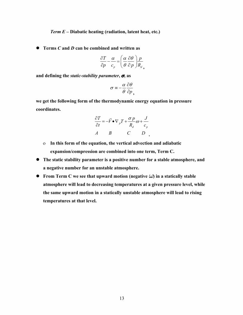
Term E – Diabatic heating (radiation, latent heat, etc.)

l Terms C and D can be combined and written as

,

and defining the static-stability parameter, s, as

,

we get the following form of the thermodynamic energy equation in pressure

coordinates.

.

o In this form of the equation, the vertical advection and adiabatic

expansion/compression are combined into one term, Term C.

l The static stability parameter is a positive number for a stable atmosphere, and

a negative number for an unstable atmosphere.

l From Term C we see that upward motion (negative ) in a statically stable

atmosphere will lead to decreasing temperatures at a given pressure level, while

the same upward motion in a statically unstable atmosphere will lead to rising

temperatures at that level.

p d

T pp c p R

a a qqæ ö¶ ¶

- = ç ÷¶ ¶è ø

p¶¶

-ºq

qas

pd p

T p JV Tt R cA B C D

s w¶= - •Ñ + +

¶

!

14

EXERCISES

1. If the atmosphere was incompressible (density constant at all altitudes), 100 km thick, and had a surface pressure of 1000 mb, at what altitude would the pressure be 250 mb? Sketch the graph of pressure vs. altitude for this case and discuss how it compares with the real atmosphere.

2. Find an expression for number density (molecules per m3) as a function of height

for a general atmosphere, and for an isothermal atmosphere.

3. Explain why airplane cabins are pressurized.

4. If the thickness of the 1000 – 500 mb layer is 5400 gpm, what is the layer average

temperature (in °C)?