Embed Size (px)
Citation preview

i
eSA-Marine - phase 1: the first step towards an operational now-cast/forecast ocean prediction
system for Southern Australia
John F. Middleton, Paul Sanderey, Charles James, Trent Mattner, Kirsten
Rough and Shane Roberts
October 2017
FRDC Project No. 2016/005
ii
© Year Fisheries Research and Development Corporation and South Australian Research and Development Institute. All rights reserved. ISBN: 978-1-876007-02-7
eSA-Marine - phase 1: the first step towards an operational now-cast/forecast ocean prediction system for Southern Australia
2016/005
2017
Ownership of Intellectual property rights Unless otherwise noted, copyright (and any other intellectual property rights, if any) in this publication is owned by the Fisheries Research and Development Corporation and the South Australian Research and Development Institute. This work is copyright. Apart from any use as permitted under the Copyright Act 1968 (Cth), no part may be reproduced by any process, electronic or otherwise, without the specific written permission of the copyright owner. Neither may information be stored electronically in any form whatsoever without such permission.
This publication (and any information sourced from it) should be attributed to Middleton, J. F., Sanderey, P., James, C., Mattner, T., Rough, K. and Roberts, S. South Australian Research and Development Institute (Aquatic Sciences) 2017. eSA-Marine - phase 1: the first step towards an operational now-cast/forecast ocean prediction system for Southern Australia. Adelaide, October.
Creative Commons licence All material in this publication is licensed under a Creative Commons Attribution 3.0 Australia Licence, save for content supplied by third parties, logos and the Commonwealth Coat of Arms.
Creative Commons Attribution 3.0 Australia Licence is a standard form licence agreement that allows you to copy, distribute, transmit and adapt this publication provided you attribute the work. A summary of the licence terms is available from creativecommons.org/licenses/by/3.0/au/deed.en. The full licence terms are available from creativecommons.org/licenses/by/3.0/au/legalcode.
Inquiries regarding the licence and any use of this document should be sent to: [email protected]
Disclaimer The authors warrant that they have taken all reasonable care in producing this report. The report has been through the SARDI internal review process, and has been formally approved for release by the Research Chief, Aquatic Sciences. Although all reasonable efforts have been made to ensure quality, SARDI does not warrant that the information in this report is free from errors or omissions. SARDI does not accept any liability for the contents of this report or for any consequences arising from its use or any reliance placed upon it. Material presented in these Administrative Reports may later be published in formal peer-reviewed scientific literature.
The information, opinions and advice contained in this document may not relate, or be relevant, to a readers particular circumstances. Opinions expressed by the authors are the individual opinions expressed by those persons and are not necessarily those of the publisher, research provider or the FRDC.
The Fisheries Research and Development Corporation plans, invests in and manages fisheries research and development throughout Australia. It is a statutory authority within the portfolio of the federal Minister for Agriculture, Fisheries and Forestry, jointly funded by the Australian Government and the fishing industry.
Researcher Contact Details FRDC Contact Details
Name:
Address:
Phone:
Fax:
Email:
John Middleton
2 Hamra Ave. West Beach, S.A. 5024
0400 037 130
08 8207 5406
Address:
Phone:
Fax:
Email: Web:
25 Geils Court
Deakin ACT 2600
02 6285 0400
02 6285 0499
www.frdc.com.au
In submitting this report, the researcher has agreed to FRDC publishing this material in its edited form.
iii
Table of Contents
Contents .............................................................................................................................. iii
Acknowledgments ............................................................................................................... v
Abbreviations ....................................................................................................................... v
The eSA-Marine web site and URL links ........................................................................... vi
Executive Summary ........................................................................................................... vii
1. Introduction .............................................................................................................. 1
1.1 Background ................................................................................................................ 1
1.2 Need .......................................................................................................................... 1
2. Objectives ................................................................................................................. 3
3. Methods - the nested approach ...................................................................................... 4
4. Results and Discussion ........................................................................................... 6
4.1 Accessing model results and the eSA-Marine web page ............................................ 6
4.2 Results: SAROM validated against observational data ............................................... 9
4.3 Results: addressing the needs of fisheries and aquaculture ....................................... 9
5. Conclusions ............................................................................................................ 11
6. Implications ............................................................................................................ 12
7. Recommendations and further development: Phase II ....................................... 13
8. Extension and Adoption ........................................................................................ 14
9. Project materials developed .................................................................................. 14
10. References .............................................................................................................. 15
Appendix A: TGM and SAROM model details. ................................................................. 16
Appendix B: Optimal ship routing .................................................................................... 18
Appendix C: eSA-Marine and web page survey ............................................................... 26
iv
Tables
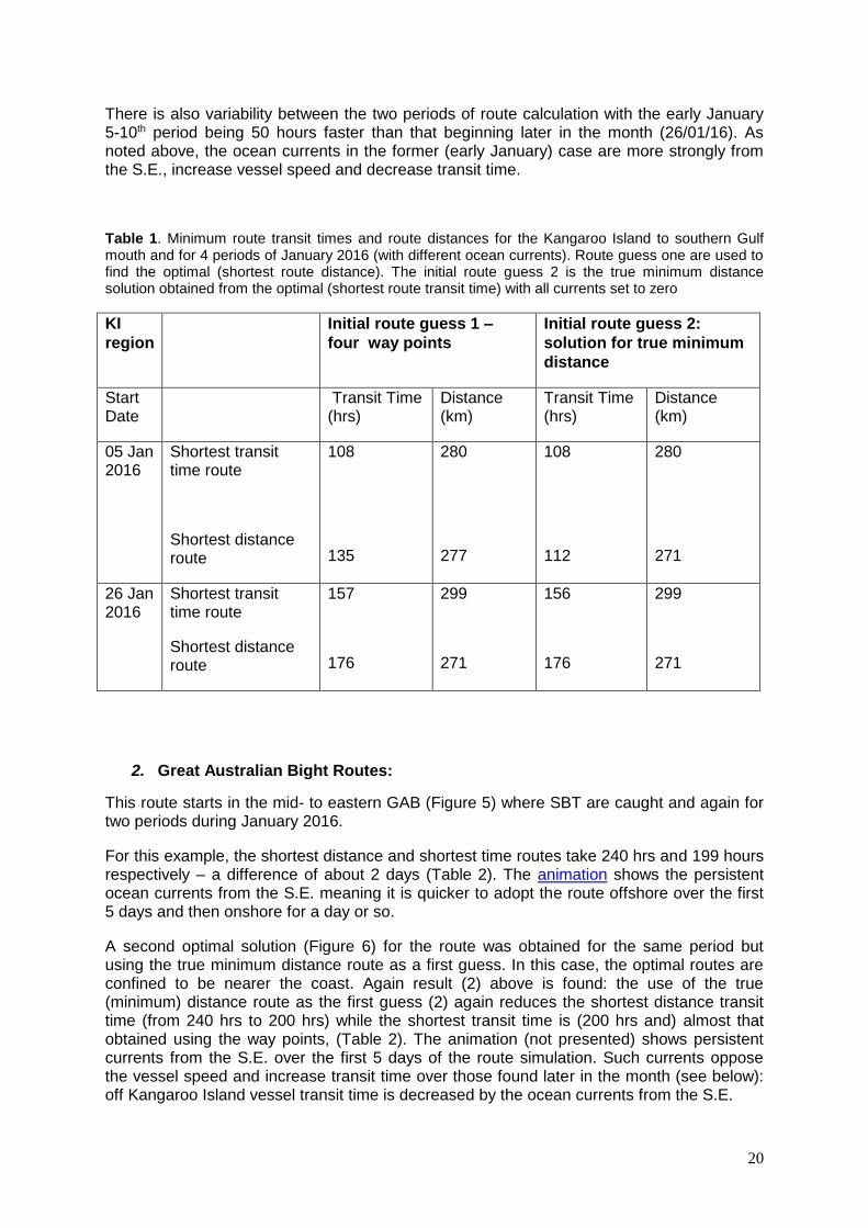
Table 1. Minimum route transit times and route distances for the Kangaroo Island to southern Gulf mouth and for 4 periods of January 2016 (with different ocean currents). Route guess one are used to find the optimal (shortest route distance). The initial route guess 2 is the true minimum distance solution obtained from the optimal (shortest route transit time) with all currents set to zero .............................................................................. 20
Table 2. Minimum route transit times and route distances for the eastern GAB to the southern Gulf mouth and for 2 periods of January 2016 (with different ocean currents). Initial route guess 1 (the way points) are used to find the optimal (shortest route distance). The initial route guess 2 is the true minimum distance solution obtained from the optimal (shortest route transit time) with all currents set to zero. ..................................................... 24
Figures
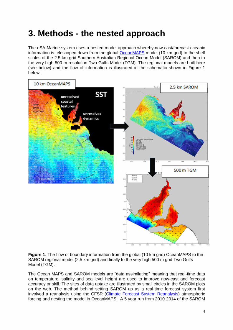
Figure 1. The above shows the flow of boundary information from the global (10 km grid) OceanMAPS to the SAROM regional model (2.5 km grid) and finally to the very high 500 m grid Two Gulfs Model (TGM). ................................................................................................ 4
Figure 2. SAROM SST and surface current now-cast on 15th September 2017. The colour bar refers to SST and a vector arrow of 50 cm/s provides a scale for currents in the figure. . 6
Figure 3. SAROM station site output at Flinders Island Outer. From the top, temperature, salinity, SSH, surface (10 m) winds and depth averaged current vectors are shown. The colour bars for T and S are self-scaling may change from figure to figure. The time axis is black for hind-casts and red for forecasts. ............................................................................ 8
Figure 4. The optimal (shortest) distance route (red) and time of passage route (green) for an initial position “A” to the mouth of the Gulf. The shortest distance and shortest time routes take 134 hrs and 108 hours respectively. The light arrows denote currents at the end of the transit and the 200 m isobath is indicated. .......................................................................... 19
Figure 5. The optimal (shortest) distance route (red) and time of passage route (green) for an initial position “A” in the GAB to the mouth of the Gulf beginning 05 January 2016 and ending 10 days later. The initial route guess is 4 way points. The light arrows denote currents at the end of the transit and the 200 m isobath is indicated. .................................. 21
Figure 6. The optimal (shortest) distance route (red) and time of passage route (green) for an initial position “A” in the GAB to the mouth of the Gulf beginning 05 January 2016 and ending 10 days later. The initial guess is the true minimum distance route. The shortest distance and shortest time routes take 201 hrs and 199 hours respectively and reflect the strong similarity of routes. The light arrows denote currents at the end of the transit and the 200 m isobath is indicated. .................................................................................................. 22
Figure 7. The optimal (shortest) distance route (red) and time of passage route (green) for an initial position “A” in the GAB to the mouth of the Gulf beginning 26th January and 2nd February 2016. The initial guess is the true minimum distance route. The shortest distance and shortest time routes take 131 hrs and 125 hrs respectively. The light arrows denote currents at the end of the transit and the 200 m isobath is indicated. .................................. 23

v
Acknowledgments
The authors thank the National Collaborative Research Infrastructure Strategy funded Integrated Marine Observing System for providing the data used in validating the eSA-Marine System and PIRSA ICT for development of the website.
Abbreviations
ACCESS-R: Australian Community Climate Earth-System Simulator Australian Bureau of Meteorology regional weather model.
ASBTIA: Australian Southern Bluefin Tuna Industry Association.
BoM: Australian Bureau of Meteorology.
BRAN 2015: Bluelink Re-Analysis (global re-analysis using OFAM) April 2009-July 2015
CSIRO: Commonwealth Scientific Industrial Research Organisation.
CTD: device to measure conductivity (salinity), depth and temperature.
NCI: National Computational Infrastructure
PIRSA: Primary Industries and Regions S.A.
POMS: Pacific Oyster Mortality Syndrome.
ROMS: Regional Ocean Modelling System.
S: ocean salinity.
SARDI: South Australian Research and Development Institute
SAROM: Southern Australian Regional Ocean Model.
SBT: Southern Bluefin Tuna.
SSH: sea surface height.
SST: sea surface temperature.
T: ocean temperature.
TGM: the Two Gulfs Model.
TPXO 8.1: Topex/Poseidon Ocean tide model.
UoA: University of Adelaide.

vi
The eSA-Marine website and URL links
The companion eSA-Marine System website is located at
http://www.pir.sa.gov.au/research/esa_marine
and should be browsed in conjunction with this report. In addition, the eSA-Marine website contains much explanatory material and is indicated by words with URL web links that are blue and underlined.

vii
Executive Summary
Background
The enhanced sustainability and profitability of fisheries and aquaculture depends on the successful management of threats that arise from toxins, viruses and harmful algal blooms. Trajectory forecasts of such hazards are needed to provide time for adequate management response (e.g., shifting tuna pens). A forecast of ocean weather (currents, waves and sea level) will also assist in the scheduling of maintenance of marine infrastructure (e.g., finfish pens) and be of use to professional and recreational divers and fishers, and mariners more generally.
Reducing vessel time costs to fisheries and aquaculture is also of importance and examples include a better knowledge of target fish habitat and optimal routing of vessels to take advantage of ocean currents.
What the report is about: aims and objectives
In all cases above, there is a need for accurate now-casts and forecasts of ocean currents, temperature and sea level. To this end, and for the first time, we aim to construct a high-resolution, now-cast/forecast system for ocean currents, temperature and sea level for Australia’s southern shelves and with a focus on the needs of fisheries and aquaculture. The system is meant as a “phase 1” system that can be used in both real-world applications, and to provide a demonstration product to explore further developments needed to support southern Australia’s fisheries and aquaculture.
Methodology
The eSA-Marine system adopts data assimilation, where real time satellite sea surface temperature (SST) and sea surface height (SSH) are used to improve the predictions of the system. An additional feature is that three models are used to telescope information down from a 10 km grid global model (OceanMAPS), to a 2.5 km grid shelf model [the Southern Australian Regional Ocean Model (SAROM)] and finally, to the 500 m scales of the Two Gulfs Model (TGM) needed to provide predictions at the scales of oyster leases and finfish pens. The system predictions are in good agreement with data from ocean moorings and field surveys.
Results - Implications
The eSA-Marine system now-casts and forecasts are available on the web at:
http://www.pir.sa.gov.au/research/esa_marine. The website contains several illustrations and scenario studies of how the results have and can be used to assist fisheries and aquaculture. It should be read in conjunction with this report. Two key results and implications are:
Pathogen trajectories: these have been determined for three scenarios using the TGM and are presented in the web site. It is planned that these will progress to simulate Pacific Oyster Mortality Syndrome (POMs) and Harmful Algal Blooms outbreaks in “trial” response exercises led by PIRSA Fisheries and Aquaculture: implication - allow for mitigation (e.g., move pens/shellfish leases).
Pelagic fish habitats: For Southern Bluefin Tuna (Thunnus maccoyii), the now-cast/forecasts of surface and bottom ocean temperature in the eastern Great Australian Bight have provided information to the Australian Southern Bluefin Tuna

viii
Industry Association (ASBTIA) for likely habitats (18 - 20 OC) during the December-March period of 2015-2016. Temperature and salinity now-casts/forecasts have also been used by industry for this period to assist with the likely locations of Australian Sardines (Sardinops sagax): implication - save fuel/time.
Other applications of the now-cast/forecast system are detailed in Section 4.3 and include origins of mass fish mortalities, lobster pot retrieval, ocean weather, optimal ship routing and fundamental fisheries and oceanographic research.
There are several other non-fisheries marine applications ranging from storm surge prediction to sea level effects on marine harbor usage and search and rescue.
Recommendations
A more accurate and useful phase II eSA-Marine System will involve several improvements of that presented here; a) further tests of model accuracy; b) on-time now-casts; c) inclusion of the effects of wind and waves in the optimal ship routing; d) inclusion of Coffin Bay (important to oyster aquaculture); and e) graphical output.
These and other recommendations are detailed in Section 7
Keywords
Ocean forecasting, now-cast/forecast systems, Australia’s southern shelves, Southern Bluefin Tuna (Thunnus maccoyii), Yellowtail Kingfish (Seriola lalandi), Australian Sardines
(Sardinops sagax), Pacific Oyster (Magallana gigas), Blacklip Abalone (Haliotis rubra),
Southern Rock Lobster (Jasus edwardsii), Western King Prawn (Penaeus [Melicertus] latisulcatus)
1
1. Introduction
1.1 Background
In this project, a pilot ("phase I") ocean forecasting system (eSA-Marine) was developed to describe the ocean state and currents both as now-casts (best estimate of the ocean conditions at the time) and forecasts (prediction of the future ocean conditions). Regional ocean forecast systems are being run in many regions of the world (e.g., Chesapeake Bay, Oregon) as they provide information to assist in the management of ports and harbours, ship routing, search and rescue, and oil spill/toxin trajectories. Because of their recognised importance to managing the marine environment, such systems form part of the Bureau of Meteorology (BoM) 2014 - 2019 marine strategy as well as the Australian National Marine Science Plan 2015-2025: driving the developments of Australia's blue economy (Recommendation 4), (Gunn, 2015).
At present, the BoM and the Commonwealth Scientific Industrial Research Organisation (CSIRO), maintain and develop the global now-cast/forecast version of BLUElink known as OceanMAPS (2015). This ocean model is 'operational', meaning it is supported 24/7 and all year round and in addition, is data assimilating: real time information on sea surface height (SSH) and sea surface temperature (SST) are used to obtain the highest skill possible for predictions. In turn, this relatively coarse grid model (~10 km), is being used to "drive" a finer resolution, now-cast/forecast regional model for the Great Barrier Reef (Sanderey et al., 2014; eReefs, 2015).
Uniquely, and in collaboration with the BoM, this project has developed a pilot now-cast/forecast ocean modelling system (eSA-Marine-phase 1) similar to eReefs but with a focus on the needs of fisheries and aquaculture for the southern Australian region. Two fine resolution coastal ocean models developed and tested by the South Australian Research and Development Institute (SARDI) are adopted here. The first is the Southern Australian Regional Ocean Model (SAROM), which is a 2.5 km grid coastal model suitable for the shelves. As part of this project, this model has been extended to include data assimilation. The second is a 500 m grid model of Spencer Gulf (Middleton et al., 2013), which has been extended to include Gulf St Vincent to form the Two Gulfs Model (TGM). These two regional models along with the global OceanMAPS model, form the basis of the eSA-Marine phase I system here. The forecast ocean system will complement that developed for winds and waves by the BoM (MetEye 2016).
It is noted that the BoM's operational seasonal forecasting system (the Predictive Ocean-Atmosphere Model for Australia) has been developed to assist in the planning and fishing operations of the ASBTIA (Eveson et al., 2015). The application of this system is over long, multi-week to seasonal time-scales with 100-200 km spatial scales that are unable to resolve important coastal physics such as upwelling events. The higher spatial resolution eSA-Marine system will provide more detailed forecasts of currents, temperature and SSH at 1 to 7 day time-scales and at 500 to 2500 m spatial scales. The two systems will thus function in a complementary manner, bridging the gap from shorter synoptic to longer seasonal time-scales.
1.2 Need
In consultation with industry, several key needs of fisheries and aquaculture may be summarised as:
2
1) Pathogen trajectories: The predicted trajectories of viruses, pollutants and harmful algal blooms that can threaten marine life as well as important aquaculture industries such as finfish, oysters, and abalone. A routinely operating prediction system with forecasting ability will allow for an improved emergency response capability such as moving finfish sea cages or oyster baskets to safer regions and better informed mitigation strategies.
2) Habitats: The distributions of important wild fish species (e.g., Australian Sardines, SBT) and their larvae are linked to biological and physical parameters (e.g., temperature/fronts). Forecasts of these parameters and thus likely wild fish habitat, will allow better directed and more economical and efficient fishing efforts. Temperature and salinity now-casts/forecasts may assist with identifying the likely locations of Australian Sardines (Doubell et al., 2015). Now-casts of temperature fronts and upwelling may also be important to tuna and other pelagic fish habitat, (Takano et al., 2009).
3) Mass fish mortalities: Information on possible origins of mass fish mortalities (anthropogenic or natural).
4) Ocean weather: Predictions of ocean weather including currents, waves and wind will enable better planning for activities such as aquaculture pen maintenance.
5) Fisheries research: Through storage of the reanalysis fields, the system will build a backlog of hind-casts that can be used to determine the likely impact of oceanographic conditions on fisheries such as the West Coast Prawns, Southern Rock Lobster (Jasus edwardsii), and/or larval dispersal of important species such as King George Whiting (Sillaginodes punctatus).
6) Optimal ship routing: The prediction of ocean currents will provide information to help optimise ship path routes (shortest time or distance) for the ASBTIA fleet when towing large pens of tuna from the shelf into Spencer Gulf and Port Lincoln.
How these needs can be addressed is outlined in Section 4.3 below. Other non-fisheries applications include ports and harbor management, search and rescue, and storm surge prediction.

3
2. Objectives
1) Develop a phase 1, demonstration now-cast/forecast system (including web delivery) for ocean currents, temperature and sea level for the southern Australian shelves, gulfs and bays that addresses the needs of industry (fisheries, aquaculture) and government.
2) Key stakeholders trained in the use and interpretation of now-casts/forecast results delivered by the investigators or website.
3) Determine and document future improvements to improve delivery of needs and model skill to provide a basis for a future Phase 2 of the now-cast/forecast system.
4) Build a hind-cast ocean circulation climatology that will be of future use in understanding the oceanographic influences on fisheries.
The achievement of these objectives is detailed below and in Section 5 (Conclusions).
4
3. Methods - the nested approach
The eSA-Marine system uses a nested model approach whereby now-cast/forecast oceanic information is telescoped down from the global OceanMAPS model (10 km grid) to the shelf scales of the 2.5 km grid Southern Australian Regional Ocean Model (SAROM) and then to the very high 500 m resolution Two Gulfs Model (TGM). The regional models are built here (see below) and the flow of information is illustrated in the schematic shown in Figure 1 below.
Figure 1. The flow of boundary information from the global (10 km grid) OceanMAPS to the SAROM regional model (2.5 km grid) and finally to the very high 500 m grid Two Gulfs Model (TGM).
The Ocean MAPS and SAROM models are “data assimilating” meaning that real-time data on temperature, salinity and sea level height are used to improve now-cast and forecast accuracy or skill. The sites of data uptake are illustrated by small circles in the SAROM plots on the web. The method behind setting SAROM up as a real-time forecast system first involved a reanalysis using the CFSR (Climate Forecast System Reanalysis) atmospheric forcing and nesting the model in OceanMAPS. A 5 year run from 2010-2014 of the SAROM
5
model was first carried out to generate a background ensemble of model error covariances. The reanalysis was then run over the same period using a sequential 3 day analysis-forecast cycle. Assimilated observations were the same as used in Bluelink ReANalysis (BRAN) 2015, which were satellite altimetry, satellite SST and in-situ temperature and salinity from Argo floats. The system was set up to use all forward independent observations for validation prior to assimilation in the next cycle in order to generate robust forecast error metrics for system performance. The system was then transferred to a scheduled real-time ‘research’ system, running at the BoM’s NCI supercomputer, by nesting it inside OceanMAPS, being forced by ACCESS-R and assimilating the real-time observations. Note the SAROM model was extended to be data assimilating as an additional in-kind contribution to this project. The SAROM real-time system runs a new forecast every 6 hours following the operational ACCESS-R schedule and takes advantage of the most recently available observations arriving at the BoM.
The SAROM model while adequate for the shelves, is used to provide open boundary information for the TGM so that features within the Gulfs (e.g., Boston Bay) are adequately resolved. Both the SAROM and TGM are forced with the best atmospheric now-cast/forecast (ACCESS-R) data available from the BoM (heating, evaporation, winds, atmospheric pressure) as well as the major tides from a global model (TPXO 8.1). The TGM is run for 4 days intervals only (due to lack of computational power), but is able to give a forecast that generally corresponds to a real-time now-cast.
Both SAROM and TGM use the hydrodynamic open source Regional Ocean Modelling System (ROMS) with 30 levels in the vertical. The TGM uses 680 X 790 cells in the horizontal while SAROM uses 439 X 270 cells. The TGM therefore takes much longer to run. Numerical model details of SAROM and the TGM are listed in Appendix A.
6
4. Results and Discussion
4.1 Accessing model results and the eSA-Marine web page
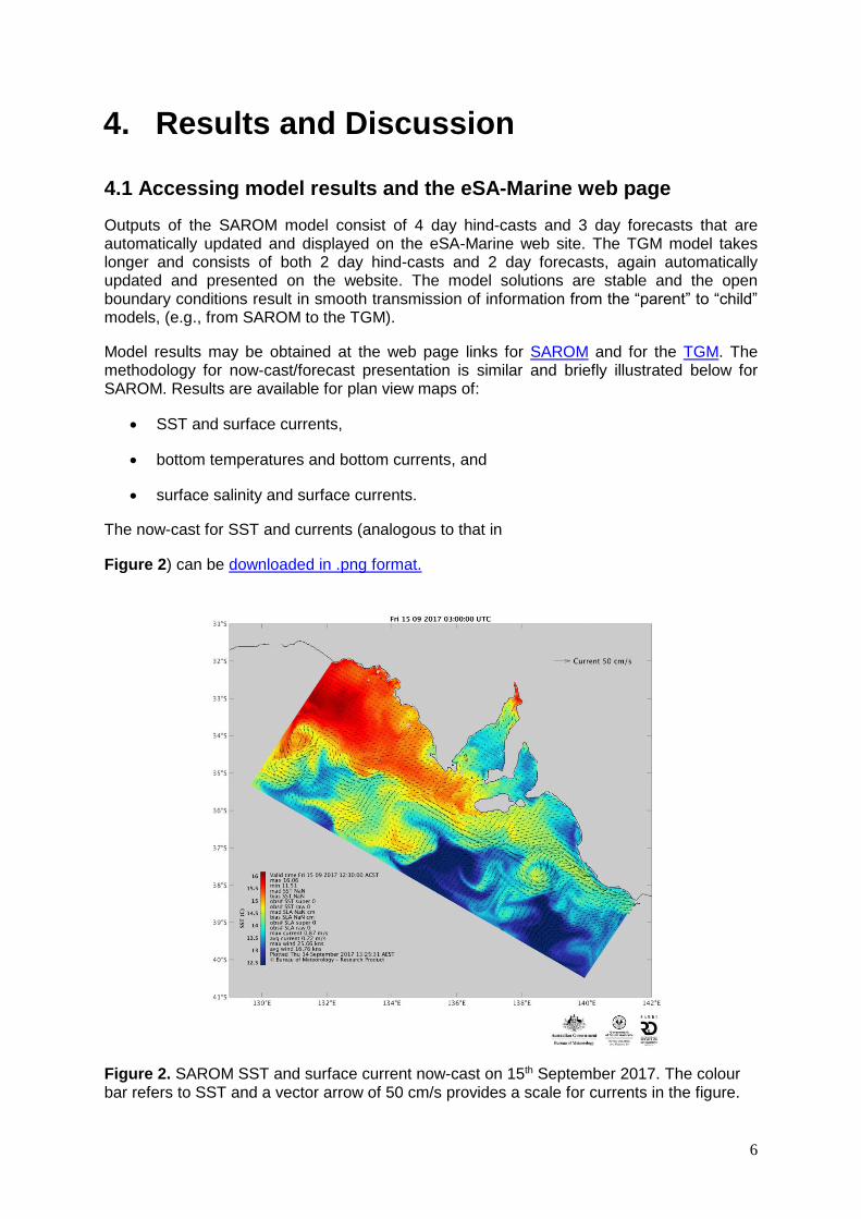
Outputs of the SAROM model consist of 4 day hind-casts and 3 day forecasts that are automatically updated and displayed on the eSA-Marine web site. The TGM model takes longer and consists of both 2 day hind-casts and 2 day forecasts, again automatically updated and presented on the website. The model solutions are stable and the open boundary conditions result in smooth transmission of information from the “parent” to “child” models, (e.g., from SAROM to the TGM).
Model results may be obtained at the web page links for SAROM and for the TGM. The methodology for now-cast/forecast presentation is similar and briefly illustrated below for SAROM. Results are available for plan view maps of:
SST and surface currents,
bottom temperatures and bottom currents, and
surface salinity and surface currents.
The now-cast for SST and currents (analogous to that in
Figure 2) can be downloaded in .png format.
Figure 2. SAROM SST and surface current now-cast on 15th September 2017. The colour bar refers to SST and a vector arrow of 50 cm/s provides a scale for currents in the figure.
7
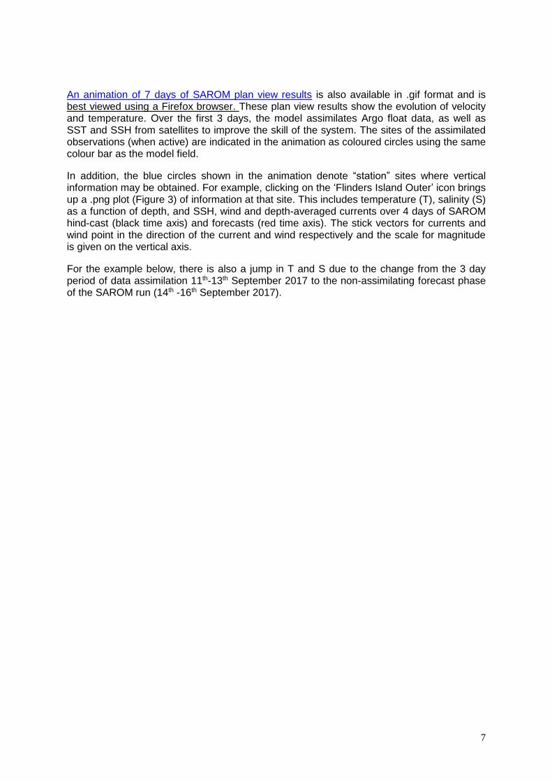
An animation of 7 days of SAROM plan view results is also available in .gif format and is best viewed using a Firefox browser. These plan view results show the evolution of velocity and temperature. Over the first 3 days, the model assimilates Argo float data, as well as SST and SSH from satellites to improve the skill of the system. The sites of the assimilated observations (when active) are indicated in the animation as coloured circles using the same colour bar as the model field.
In addition, the blue circles shown in the animation denote “station” sites where vertical information may be obtained. For example, clicking on the ‘Flinders Island Outer’ icon brings up a .png plot (Figure 3) of information at that site. This includes temperature (T), salinity (S) as a function of depth, and SSH, wind and depth-averaged currents over 4 days of SAROM hind-cast (black time axis) and forecasts (red time axis). The stick vectors for currents and wind point in the direction of the current and wind respectively and the scale for magnitude is given on the vertical axis.
For the example below, there is also a jump in T and S due to the change from the 3 day period of data assimilation 11th-13th September 2017 to the non-assimilating forecast phase of the SAROM run (14th -16th September 2017).
8
Figure 3. SAROM station site output at Flinders Island Outer. From the top, temperature, salinity, SSH, surface (10 m) winds and depth averaged current vectors are shown. The colour bars for T and S are self-scaling may change from figure to figure. The time axis is black for hind-casts and red for forecasts.

9
4.2 Results: SAROM validated against observational data
a) Satellite Data (SST and SSH):
A historical reanalysis was run over a 5 year period (2010-2014) on a three day assimilation cycle. This re-analysis represents the “best” solution for the estimated currents, temperature, salinity, etc. To obtain the re-analysis, the modelling system is run as a long time series of short forecasts where each forecast is compared to all available satellite observations (SST and SSH), prior to assimilation into the next analysis. This enables forecast statistics to be generated in order to assess overall system performance, check how well the model can be constrained to the observations and assess the stability and reliability of the system. The ocean forecasts have been shown to match the observations (after the fact) and therefore provide useful information about the future state of the ocean. The SAROM re-analysis was stored as daily averages so as to provide a climatological time series of the best available historical estimate of the ocean state. For the summary of forecast errors from the re-analysis refer to Figure 1 and Table 1 in the Model Validation section on the eSA-Marine website.
b) Comparison with IMOS and other data:
Velocity, temperature and salinity data were collected from the Southern Australian Integrated Marine Observing System (SAIMOS) including moorings and field surveys. Time series plots of the major axis current meter data and that obtained from the SAROM re-analysis data set were compared for several sites and the model output shown to be able to reproduce weather band currents and vertical shear. Monthly averaged model currents were found to over-estimate the data by up to 10 cm/s during winter but show good agreement during summer. Good agreement was found between snapshots of (T, S) data and model output, during both summer upwelling in February 2012 and winter downwelling in May 2014. This illustrates that the model is well able to reproduce the important processes of upwelling and downwelling.
c) Port Pirie Storm Surge:
Both the SAROM and the TWG in forecast mode were able to re-produce the tidal variability and the 29 September 2016 storm surge event at Port Pirie. The forecast was made 2 days prior to the storm surge and reproduced the observed tidal SSH and the 5 m amplitude and timing of the Port Pirie surge.
4.3 Results: addressing the needs of fisheries and aquaculture
1) Pathogen trajectories: these have been determined for three scenarios using the TGM and are presented in the website. It is planned that these will progress to simulated POMs and harmful algal blooms outbreaks in response exercises led by PIRSA Fisheries and Aquaculture.
2) Pelagic fish habitats: For SBT, the now-cast/forecasts of surface and bottom ocean temperature in the eastern Great Australian Bight have already provided information to the ASBTIA for likely habitats (18 - 20 OC; Eveson et al., 2015) during the December-March period of 2015-2016. Temperature and salinity now-casts/forecasts may also assist with identifying the likely locations of Australian Sardines (Doubell et al., 2015).

10
3) Mass fish mortalities: After such events, the models can be re-run to back track from locations of dead fish to see if a common spatial origin was likely, which could help ascertain possible cause.
4) Ocean weather: The now-cast/forecast of ocean currents of eSA-Marine complement the BoM's existing web based system for surface waves and marine winds (MetEye): these are easily accessible from the home page of the eSA-Marine web site. The net result is a now- cast/forecast model for ocean "weather" that will be of use for aquaculture maintenance, recreational and professional fishers/divers and a wide range of other marine activities.
5) Fisheries and Oceanographic research: the SAROM model re-analysis (daily averaged) outputs have been stored since 2010 and will be an invaluable resource for future fisheries and oceanographic research.
6) Optimal ship routing: Several scenario studies were undertaken using the SAROM reanalysis climatology of surface currents so as to minimise transit time from, for example, the west coast to Port Lincoln and subject to a constraint of a constant vessel speed through the water [e.g., 1 knot for SBT pen towing]. Several such studies are detailed in Appendix B and an example is given on the eSA-Marine website.
A second objective of the project was to ensure key stakeholders were trained in the use and interpretation of now-casts/forecasts and the website. This was achieved through presentations made to the ASBTIA and other fisheries associations (e.g., Rock Lobster). A formal survey was also undertaken after a presentation made at SARDI (18 July 2017) to evaluate industry and government needs and the utility of the web site. The results of the survey were positive and are presented in Appendix C.
11
5. Conclusions
In line with Objective 1, a stable (partially validated) now-cast/forecast system has been developed for Australia’s southern shelves and gulfs and is delivered through the eSA-Marine website:
http://pir.sa.gov.au/research/esa_marine
The system adopts data assimilation for the shelf scale SAROM model, which was not foreshadowed in the original proposal where a standard hydrodynamic model was to be used for SAROM. The use of assimilation in SAROM provides more accurate now-casts and forecasts and also boundary forcing for the TGM. Further model validation is however needed to determine where or when good model skill is or is not obtained and the reasons for this.
Objective 2 was to ensure adequate training of industry in the use and interpretation of eSA-Marine. Explanations of SAROM now-casts/forecasts were given to ASBTIA at their November 2016 research meeting and followed up by discussions on the use of SAROM output in tuna school spotting. A formal survey was undertaken in July 2017 and the summary report provided largely positive feedback (see Appendix C).
The third objective, outlining the improvements needed for the second phase of eSA-Marine, was achieved and these are detailed in Section 7.
Finally, the fourth objective was completed through the collation of the SAROM reanalysis output as daily averages for 2010 to 2016.
12
6. Implications
The eSA-Marine system and website should allow for better management of fisheries and aquaculture, as well as cost savings to industry.
This is particularly the case for the use of the now-casts/forecasts in the areas of pathogen/virus trajectory prediction, identification of likely pelagic fish habitats (e.g., SBT) and ocean weather prediction. The benefits are to industries, government management and professional and recreational divers and fishers.
Optimal ship routing for the towing of juvenile SBT pens has been identified as an area of potential importance. The inclusion of the effects of winds and waves is needed and further collaboration with ASBTIA to proof the utility of this application. For the scenario studies made (Appendix B), savings of 10-20% of transit time may lead to substantial cost savings to ASBTIA and other marine industry groups.
The climatology of the SAROM re-analysis fields should prove useful to further fisheries and oceanographic research.
Finally, the eSA-Marine products can be of benefit in non-fisheries applications including storm surge prediction, harbor management and search and rescue.

13
7. Recommendations and further
development: phase II
In this project, the first phase of a now-cast/forecast system was developed for the southern shelves with the aim to provide real-time information via the website to assist fisheries and aquaculture.
There are a number of limitations that require further development in a phase II system that will require additional funding.
1) Model accuracy:
a) This has only been demonstrated through limited comparisons with data and more extensive comparisons are required with oceanographic data.
b) This needs to be improved in the TGM by adoption of data assimilation.
2) On-time now-casts. The TGM take 9 hours to compute a 4 day run of the TGM model output. Therefore, the TGM now-cast is typically 24 hours late. This could be rectified by use of a computer that is 3 to 4 times faster than that currently used.
3) Model storage. The extensive SAROM re-analysis product is stored as daily averages by the BoM on its extensive super-computer system. Options for storing the TGM output need to be found. At present the TGM needs to be re-run to reproduce anything but the daily now-cast/forecasts.
4) An interactive website. Currently, the eSA-Marine web site is non-interactive meaning, only pre-loaded images and output can be accessed and the website cannot be used to interrogate the numerical model outputs. The extension to an interactive website remains a goal of phase II.
5) In the original proposal, a high-resolution model of Coffin Bay was to be included in eSA-Marine. However, due to the computational costs of the TGM, the Coffin Bay model (while developed) is not currently run. Moreover, further research is needed to derive the correct coupling of the very small mouth of Coffin Bay (1.5 km) to the 2.5 km grid of the SAROM model.
6) Graphical output. Software is needed to allow the user to determine (latitude, longitude) and variable values through a right click of the mouse on plan view figures (as done in Google Earth). This problem is under active consideration.
7) Consult with the broader fishing industry on further possible applications; e.g., allow lobster fishers to determine from the eSA-Marine website if their pot surface floats have been driven underwater by strong currents and when they will re-appear to retrieve lobster catch.
8) Extend the optimal ship routing to more accurately include forcing by winds and waves.
9) Include plots of bottom topography.

14
8. Extension and Adoption
Since November 2016, presentations and discussions have been made with South Australian industries including ASBTIA, the Sardine and Rock Lobster Industry Associations, and presentations given to the Australasian Aquatic Health Conference (July 2017) and the national Forum on Operational Oceanography (July 2017). A seminar was given at SARDI (18 July 2017) to local government, industry and scientists. Early SAROM results were adopted by ASBTIA and the Sardine industry in January-March this year.
9. Project materials developed
The URL of the eSA-Marine website is http://pir.sa.gov.au/research/esa_marine and should be referenced on the FRDC website.

15
10. References
Bijlsma, S. J. (2010). Optimal Ship Routing with Ocean Current Included. Journal of Navigation, 63(03), 565{568.doi:10.1017/S0373463310000159.
Chapman, D. C. (1985). Numerical treatment of cross-shelf open boundaries in a barotropic coastal ocean model, J. Phys. Oceanogr., 15, 1060 -1075. Doubell, M. J., et al., (2015). Optimising the size and quality of Sardines through real-time harvesting. Prepared by the SARDI Aquatic Sciences), Adelaide. CRC Project No. 2013/747. 47pp. Egbert, G.D., and S.Y. Erofeeva (2002). Efficient inverse modelling of barotropic ocean tides, J. Atmos. Oceanic Technol., 19(2), 183-204.
Gunn, J. and National Marine Science Committee (Australia) (2015). National Marine Science Plan 2015-2025: driving the development of Australia's blue economy. [Canberra]
eReef (2015). http://www.bom.gov.au/environment/activities/coastal-info.shtml Eveson, J. P., et al., (2015). Seasonal forecasting of tuna habitat in the Great Australian Bight (2015), Fisheries Res., 170, 39-49. Flather, R. A. (1976). A tidal model of the northwest European continental shelf, Memoires de la Societe Royale de Sciences de Liege, 6, 141-164. Large, W.G., J.C. McWilliams, and S.C. Doney (1994). A Review and model with a nonlocal boundary layer parameterization, Reviews of Geophysics, 32, 363-403. MetEye (2016). http://www.bom.gov.au/australia/meteye/ Middleton, J., et al. (2013). PIRSA Initiative II: carrying capacity of Spencer Gulf: hydrodynamic and biogeochemical measurement modelling and performance monitoring. Final Report for the FRDC. South Australian Research and Development Institute (Aquatic Sciences), Adelaide. SARDI Publication No. F2013/000311-1. SARDI Research Report Series No. 705. 97pp. OceanMAPS (2015). http:\www.bom.gov.au\oceanography\forecasts\index.shtml
Sandery P. A., P. Sakov and L. Majewski (2014). The impact of open boundary forcing on forecasting the East Australian Current using ensemble data assimilation, Ocean Modelling, 84, 1-11. Takano, A. et al., (2009). A method to estimate three-dimensional thermal structure from satellite altimetry data. J. Atmos. And Oceanic Tech .26, 2655-2664.

16
Appendix A: TGM and SAROM model
details.
Numerical component TGM SAROM
Now-cast/forecast interval 4 days 7 days
Name of grid grd_GULFS_500m.nc grd_eSAM_20160707.nc
Size of grid 680x790X30 439x270x30
~Horizontal grid cell size 500 m 2.5 km
Horizontal coordinate system
Spherical Orthogonal curvilinear grid
Vertical coordinate system Sigma terrain following Sigma terrain following
Bottom drag formulation Quadratic bottom stress Quadratic bottom stress
Vertical mixing parameterisation
LMD parameterisation,
Large et al. (1994)
K-Profile parameterisation,
Large et al. (1994)
Horizontal eddy viscosity coefficient
10 m2/s 2 m2/s
Horizontal mixing coefficient for temperature and salt
0 m2/s 0 m2/s – this is because the 3rd order upwind horizontal advection scheme in ROMS, which is the most robust high order one available, is still slightly diffusive.
Bathymetric data set Geosciences Australia Geosciences Australia
Initial conditions (T, S, u, v, U, V)
SAROM OceanMAPS T,S
Open boundary nesting:
T & S source
Width of nudging layer
Time scale at boundary
Time scale at interior
SAROM
N/A
1 day inflow, 360 days outflow
N/A
T,S,U,V,SSH
OceanMAPS
N/A: No nudge layer
1 day inflow, 360 days outflow
N.A.
Open boundary condition:
source
SAROM
17
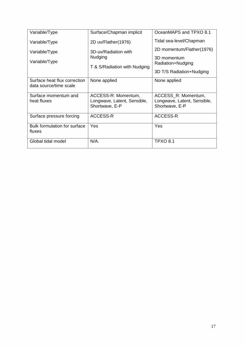
Variable/Type
Variable/Type
Variable/Type
Variable/Type
Surface/Chapman implicit
2D uv/Flather(1976)
3D-uv/Radiation with Nudging
T & S/Radiation with Nudging
OceanMAPS and TPXO 8.1
Tidal sea-level/Chapman
2D momentum/Flather(1976)
3D momentum Radiation+Nudging
3D T/S Radiation+Nudging
Surface heat flux correction data source/time scale
None applied None applied
Surface momentum and heat fluxes
ACCESS-R: Momentum, Longwave, Latent, Sensible, Shortwave, E-P
ACCESS_R: Momentum, Longwave, Latent, Sensible, Shortwave, E-P
Surface pressure forcing ACCESS-R ACCESS-R
Bulk formulation for surface fluxes
Yes Yes
Global tidal model N/A. TPXO 8.1

18
Appendix B: Optimal ship routing
Optimisation theory (e.g., Bijlsma 2010) allows estimates of the quickest and shortest routes for vessels to transit from points A to B in the presence (or absence) of ocean currents: the theory and application adopted here is well developed in the context of the effects of winds and waves on ocean vessel routes. Such routes may result in significant savings in fuel and time for the case of the Southern Bluefin Tuna (SBT) industry where large schools of juvenile SBT are caught on the shelf, penned, and then slowly towed back to the ranching areas near Port Lincoln to be grown and conditioned for the market.
Indeed, of particular interest here are the routes that can be determined for a vessel that is
constrained to move (no faster) than a speed V (1 knot or ~0.5 m/s) relative to the ocean currents. This case is important to the tuna industry as it seems to be a speed that the fish are comfortable to swim at for extended periods of time. Also towing at higher speeds relative to the ocean currents puts greater strain on vessels and nets, which increases fuel usage and reduces integrity and lifespan of infrastructure.
In the following, several illustrative (and hypothetical) examples are shown using the
SAROM re-analysis field for surface ocean currents (U) for the summer of 2016 when fish transit the Great Australian Bight (GAB). These fields are prescribed on a 2 km grid and at 3 – hourly intervals.
The vessel is assumed to move with these ocean currents, and combined with that relative
to the water V, the total vessel velocity u and path X (t) is
u = U + V(ϴ) (1a)
dX/dt = u(x,y,t) (1b)
where the user prescribed start and end point vessel positions are X(0) = A and X(T) = B, with T the transit time calculated for the given route. The heading angle of the vessel is ϴ(t) and is determined for each part of each route by the optimization procedure for both the minimum route distance and minimum route transit time. Sometimes, it is impossible for the vessel to travel along the minimum distance route due to excessive currents. In that case, the algorithm searches for the minimum feasible distance route, which is the minimum distance route subject to those currents. An additional constraint on the solutions is that the water depth must exceed 40 m so vessels cannot “run aground”.
Initial guesses of the entire route must be given which are then perturbed using the optimisation theory and constraints above to determine the minimal distance and transit time routes and associated transit times. As will be shown, the solutions are sensitive to these initial guesses and more than one optimal route may exist.
1. Kangaroo Island Routes:
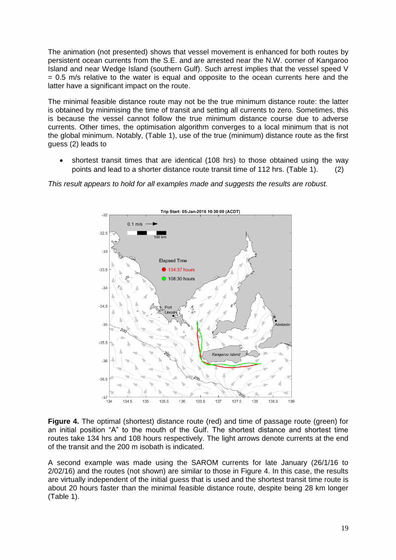
As an illustration consider the S.E. Kangaroo Island (A) to southern Spencer Gulf (B) routes shown in Figure 4. In this case, 4 way points were prescribed as a guess for the shortest route and, using the SAROM ocean currents, the “minimal feasible distance route” was determined using optimisation theory: the red route has a transit time of 135 hrs.
Minimising the transit time for the given ocean currents leads to the green route in Figure 4 with a transit time of 108 hours – a saving of 27 hours over the minimal feasible distance route.
19
The animation (not presented) shows that vessel movement is enhanced for both routes by persistent ocean currents from the S.E. and are arrested near the N.W. corner of Kangaroo Island and near Wedge Island (southern Gulf). Such arrest implies that the vessel speed V = 0.5 m/s relative to the water is equal and opposite to the ocean currents here and the latter have a significant impact on the route.
The minimal feasible distance route may not be the true minimum distance route: the latter is obtained by minimising the time of transit and setting all currents to zero. Sometimes, this is because the vessel cannot follow the true minimum distance course due to adverse currents. Other times, the optimisation algorithm converges to a local minimum that is not the global minimum. Notably, (Table 1), use of the true (minimum) distance route as the first guess (2) leads to
shortest transit times that are identical (108 hrs) to those obtained using the way
points and lead to a shorter distance route transit time of 112 hrs. (Table 1). (2)
This result appears to hold for all examples made and suggests the results are robust.
Figure 4. The optimal (shortest) distance route (red) and time of passage route (green) for an initial position “A” to the mouth of the Gulf. The shortest distance and shortest time routes take 134 hrs and 108 hours respectively. The light arrows denote currents at the end of the transit and the 200 m isobath is indicated.
A second example was made using the SAROM currents for late January (26/1/16 to 2/02/16) and the routes (not shown) are similar to those in Figure 4. In this case, the results are virtually independent of the initial guess that is used and the shortest transit time route is about 20 hours faster than the minimal feasible distance route, despite being 28 km longer (Table 1).
20
There is also variability between the two periods of route calculation with the early January 5-10th period being 50 hours faster than that beginning later in the month (26/01/16). As noted above, the ocean currents in the former (early January) case are more strongly from the S.E., increase vessel speed and decrease transit time.
Table 1. Minimum route transit times and route distances for the Kangaroo Island to southern Gulf mouth and for 4 periods of January 2016 (with different ocean currents). Route guess one are used to find the optimal (shortest route distance). The initial route guess 2 is the true minimum distance solution obtained from the optimal (shortest route transit time) with all currents set to zero
KI
region
Initial route guess 1 –
four way points
Initial route guess 2:
solution for true minimum
distance
Start Date
Transit Time (hrs)
Distance (km)
Transit Time (hrs)
Distance (km)
05 Jan 2016
Shortest transit time route
Shortest distance route
108
135
280
277
108
112
280
271
26 Jan 2016
Shortest transit time route
Shortest distance route
157
176
299
271
156
176
299
271
2. Great Australian Bight Routes:
This route starts in the mid- to eastern GAB (Figure 5) where SBT are caught and again for two periods during January 2016.
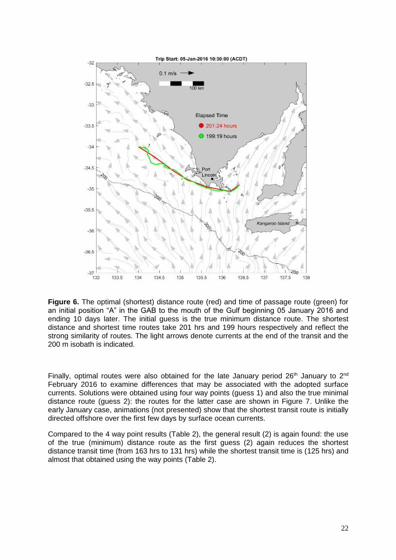
For this example, the shortest distance and shortest time routes take 240 hrs and 199 hours respectively – a difference of about 2 days (Table 2). The animation shows the persistent ocean currents from the S.E. meaning it is quicker to adopt the route offshore over the first 5 days and then onshore for a day or so.
A second optimal solution (Figure 6) for the route was obtained for the same period but using the true minimum distance route as a first guess. In this case, the optimal routes are confined to be nearer the coast. Again result (2) above is found: the use of the true (minimum) distance route as the first guess (2) again reduces the shortest distance transit time (from 240 hrs to 200 hrs) while the shortest transit time is (200 hrs and) almost that obtained using the way points, (Table 2). The animation (not presented) shows persistent currents from the S.E. over the first 5 days of the route simulation. Such currents oppose the vessel speed and increase transit time over those found later in the month (see below): off Kangaroo Island vessel transit time is decreased by the ocean currents from the S.E.

21
Figure 5. The optimal (shortest) distance route (red) and time of passage route (green) for an initial position “A” in the GAB to the mouth of the Gulf beginning 05 January 2016 and ending 10 days later. The initial route guess is 4 way points. The light arrows denote currents at the end of the transit and the 200 m isobath is indicated.
22
Figure 6. The optimal (shortest) distance route (red) and time of passage route (green) for an initial position “A” in the GAB to the mouth of the Gulf beginning 05 January 2016 and ending 10 days later. The initial guess is the true minimum distance route. The shortest distance and shortest time routes take 201 hrs and 199 hours respectively and reflect the strong similarity of routes. The light arrows denote currents at the end of the transit and the 200 m isobath is indicated.
Finally, optimal routes were also obtained for the late January period 26th January to 2nd February 2016 to examine differences that may be associated with the adopted surface currents. Solutions were obtained using four way points (guess 1) and also the true minimal distance route (guess 2): the routes for the latter case are shown in Figure 7. Unlike the early January case, animations (not presented) show that the shortest transit route is initially directed offshore over the first few days by surface ocean currents.
Compared to the 4 way point results (Table 2), the general result (2) is again found: the use of the true (minimum) distance route as the first guess (2) again reduces the shortest distance transit time (from 163 hrs to 131 hrs) while the shortest transit time is (125 hrs) and almost that obtained using the way points (Table 2).

23
Figure 7. The optimal (shortest) distance route (red) and time of passage route (green) for an initial position “A” in the GAB to the mouth of the Gulf beginning 26th January and 2nd February 2016. The initial guess is the true minimum distance route. The shortest distance and shortest time routes take 131 hrs and 125 hrs respectively. The light arrows denote currents at the end of the transit and the 200 m isobath is indicated.
24
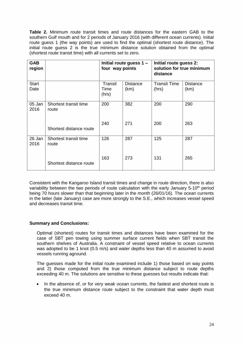
Table 2. Minimum route transit times and route distances for the eastern GAB to the southern Gulf mouth and for 2 periods of January 2016 (with different ocean currents). Initial route guess 1 (the way points) are used to find the optimal (shortest route distance). The initial route guess 2 is the true minimum distance solution obtained from the optimal (shortest route transit time) with all currents set to zero.
GAB
region
Initial route guess 1 –
four way points
Initial route guess 2:
solution for true minimum
distance
Start Date
Transit Time (hrs)
Distance (km)
Transit Time (hrs)
Distance (km)
05 Jan 2016
Shortest transit time route
Shortest distance route
200
240
382
271
200
200
290
263
26 Jan 2016
Shortest transit time route
Shortest distance route
126
163
287
273
125
131
287
265
Consistent with the Kangaroo Island transit times and change in route direction, there is also variability between the two periods of route calculation with the early January 5-10th period being 70 hours slower than that beginning later in the month (26/01/16). The ocean currents in the latter (late January) case are more strongly to the S.E., which increases vessel speed and decreases transit time.
Summary and Conclusions:
Optimal (shortest) routes for transit times and distances have been examined for the case of SBT pen towing using summer surface current fields when SBT transit the southern shelves of Australia. A constraint of vessel speed relative to ocean currents was adopted to be 1 knot (0.5 m/s) and water depths less than 40 m assumed to avoid vessels running aground.
The guesses made for the initial route examined include 1) those based on way points and 2) those computed from the true minimum distance subject to route depths exceeding 40 m. The solutions are sensitive to these guesses but results indicate that:
In the absence of, or for very weak ocean currents, the fastest and shortest route is
the true minimum distance route subject to the constraint that water depth must
exceed 40 m.
25
The use of the true (minimum) distance route as the first guess reduces the shortest
distance transit time while the shortest transit time is almost equal to that obtained
using the way points.
We conclude that the minimum transit times are robust and generally shorter than
that based on the minimum distance route.
In addition, we expect the minimum transit time routes to be increasingly shorter than
the minimum shortest distance routes for stronger and more variable ocean currents.
Ocean currents are important to determining optimal ship routes and can arrest total
vessel speed and change the transit times by 50%.
The effects of winds and waves were not examined but are known to be important and should be included in future studies. Indeed, though an extensive literature, the parameterization of the effects of winds and waves are known to depend on vessel and pen shape. The joint effects of currents, winds and waves will require further study and notably validation against observations of real vessel drift. There is much work to be done to progress this application of the eSA-Marine System.

26
Appendix C: eSA-Marine and website
survey
Informal input into improvements of the eSA-Marine system and website has been received
since development began and notably since November 2016 when the on-line SAROM now-
casts/forecasts were presented to the ASBTIA at their annual research meeting. A formal
survey (see below) was distributed and discussed in July 2017 and the responses
summarised.
Kirsten Rough (ASBTIA) discussed the system and website with key industry end users –
fishers, tuna spotters, tow skippers, tuna company managers and quota owners. Responses
are summarized below:
a) This has proven to be a very useful project that has delivered beyond the industries
expectations.
b) The individuals and companies (Executive, Management and staff at fishing and
spotter levels) are all extremely happy with how this project has delivered. Those
draft web links provided early in the project are continuing to be used by the SBT
fishers that fish for sardines for the remainder of the year – uptake has been terrific.
c) The ability to “right click” the plan view maps to get latitude and longitude would be
very useful and assist industry in getting GPS co-ordinates of regions of interest – a
feature found in Google Earth. This was not achieved in this project.
Survey Questions, Feedback and Our Response.
1) Web site easy to navigate?
Feedback: Generally yes, although “home” buttons to take one back to the home
page would help.
2) Any additional explanations needed –describe?
Feedback: The explanations are fine.
3) Additional station sites needed – pls state (latitude, longitude and short place-
name)?
Feedback: ASBTIA nominated 8 more site stations for SAROM and the TGM.
Our Response: these were adopted.
4) Any comments on the graphics - too small?
Feedback: Generally OK but one concern was the self-scaling colour bars for
temperature etc.
Our Response: these were chosen to highlight detail where large temperature
variations occur between seasons and depths. The website does indicate this
feature. We tried a fixed colour bar and at times, no detail could be found.
5) Would the ability to right click the maps to get latitude and longitude be useful?
Feedback: Yes
Our response: We have worked on the software needed but were unable to find a
solution for this phase I system.
27
6) Speed of loading of animations OK?
Feedback: OK
7) Any additional quantities to plot or overlay?
Feedback: Isotherms for 18 and 20oC were identified by ASBTIA
Our Response: incorporated.
Feedback: Sea floor topography would be desirable.
Our Response: to be an additional plot in Phase II.
8) Other likely sites for particle (toxin/HAB) dispersal?
Feedback: Would be good to have something along the shelf break for surface
currents
Our Response: Other key sites will be incorporated in some limited studies through
discussions/collaborations with PIRSA Biosecurity. Inclusion of any model site for
particle dispersion is easily made and can be initialised in any one 24 hr cycle.