Erwin Brüning School of Mathematical Sciences January 2011erwin/calovar2011.pdf · 6 CHAPTER 1. INTRODUCTION ≈ 800 B.C. Legend of Queen Dido; ﬁrst recorded solution of an isoperimetric

Calculus of Variations

An Introduction with Applications in Spectral Theory

Erwin BrüningSchool of Mathematical Sciences

January 2011

2

Contents

1 Introduction 5

1.1 History . . . . . . . . . . . . . . . . . . . . . . . . . 51.2 Classical approach and direct methods . . . . . . . 8

2 Direct methods in the calculus of variations 11

2.1 Outline of general strategy . . . . . . . . . . . . . . 132.2 General existence results . . . . . . . . . . . . . . . 162.3 Minimization in Banach spaces . . . . . . . . . . . 182.4 Minimization of special classes of functionals . . . 212.5 Exercises . . . . . . . . . . . . . . . . . . . . . . . . 23

3 Differential Calculus on Banach Spaces 25

3.1 The Fréchet derivative . . . . . . . . . . . . . . . . 263.2 Extrema of differentiable functions . . . . . . . . . 333.3 Convexity and monotonicity . . . . . . . . . . . . . 363.4 Gâteaux derivatives and variations . . . . . . . . . 393.5 Exercises . . . . . . . . . . . . . . . . . . . . . . . . 43

4 Constrained Minimization Problems 47

4.1 Geometrical interpretation of constrained mini-mization . . . . . . . . . . . . . . . . . . . . . . . . 48

4.2 Tangent spaces of level surfaces . . . . . . . . . . . 504.3 Existence of Lagrange multipliers . . . . . . . . . . 53

4.3.1 Comments on Dido’s problem . . . . . . . 554.4 Exercises . . . . . . . . . . . . . . . . . . . . . . . . 57

3

4 CONTENTS

5 Surjectivity of monotone coercive operators 59

5.1 The result of Browder and Minty . . . . . . . . . . 595.2 The proofs . . . . . . . . . . . . . . . . . . . . . . . 61

5.2.1 The proof of the Browder-Minty theorem . 615.2.2 Proof of Lemma ?? . . . . . . . . . . . . . . 635.2.3 Proof of Lemma ?? . . . . . . . . . . . . . . 64

5.3 An important variation of the Browder-Minty result 65

6 Sobolev spaces 67

6.1 Motivation . . . . . . . . . . . . . . . . . . . . . . . 676.2 Basic definitions . . . . . . . . . . . . . . . . . . . . 676.3 Morrey’s inequality . . . . . . . . . . . . . . . . . . 716.4 Gagliardo-Nirenberg-Sobolev inequality . . . . . . 74

6.4.1 Continuous Embeddings of Sobolev spaces 786.4.2 Compact Embeddings of Sobolev spaces . 80

7 Some Applications 85

7.1 Spectral Theory for compact Operators . . . . . . 857.2 Some linear boundary and eigenvalue problems . 88

7.2.1 The Dirichlet–Laplace operator . . . . . . 887.2.2 Linear elliptic differential operators . . . . 91

7.3 Some nonlinear boundary and eigenvalues prob-lems . . . . . . . . . . . . . . . . . . . . . . . . . . . 93

7.4 Generalized Dirichlet Forms and variational BVPs 1017.5 Some global problems . . . . . . . . . . . . . . . . 1037.6 Problems with critical growth . . . . . . . . . . . . 1047.7 Problems not treated here . . . . . . . . . . . . . . 104

Chapter 1

Introduction

Calculus of variations or ‘variational calculus’ is one of the old-est parts of mathematics and it has influenced the developmentof mathematics in many ways. The name for this theory goesback to L. Euler’s publication A method for finding curves enjoying

certain maximum or minimum properties in 1744. But the theoryis much older, due to its intimate relation to problems humansencountered from early days of existence, namely to find ‘opti-mal’ solutions to practical problems, for instance to “minimizelosses" and to “maximize benefits (profits)". In this wider senseof finding optimal solutions it is nearly 3000 years old (see nextsubsection).

1.1 History

Here we mention only the most important dates in the historyof variational calculus. For a concise account we recommendthe introduction to the book BB92 where one finds also furtherreferences. The following table presents some highlights:

5

6 CHAPTER 1. INTRODUCTION

≈ 800 B.C.

Legend of Queen Dido; first recordedsolution of an isoperimetric problem (i.e.,the problem of finding the curve whichencloses the largest area for a given length).

≈ 250 B.C.

ancient Greece; several extreme value prob-lems were solved, in particular it was shownthat the shortest path joining two points isthe straight line through the given points.

1662Fermat: Principle of least time for the propa-gation of light.

July 1696

birth of modern variational calculus: Johann

Bernoulli presented the brachystochrone prob-

lem in the Acta Eruditorum Lipsiae. Theproblem: A point mass glides without fric-tion along a curve joining a point A with alower point B. Which curve gives the short-est travel time if the point mass is movingonly under the influence of gravity (accord-

1.1. HISTORY 7

July 1696

ing to Newton’s law). Very soon many solu-tions were propoesed by well known math-ematicians, among them by Jakob Bernoulli,Newton, Leibniz, and l’Hopital.

1684

Leibniz - first publication on differential cal-culus: Nova methodus pro maximis et minimis

itemque tangentibus; beginning of a mathe-

matical theory of optimization.

1744

L. Euler: first textbook entitled A method

for finding curves enjoying certain maximum or

minimum properties.

1753L. Euler: Dissertatio de principio minimae

actionis.

1786

Legendre: How to distinguish stationarypoints? Second necessary condition for anextremum, in terms of ‘second variation.

1788 Lagrange: Mécanique analytique.

1837

Jacobi: Theory of variational calculus and differ-

ential equations; completed Legendre’s studyon the second variation.

≈ 1850

Dirichlet problem: Dirichlet and Riemanntook the existence of extreme value problemsfor granted, thus ‘solving’ the Dirichlet prob-

lem: Find a solution to the potential equation

u = 0 in G,

G ⊂ R2, with given values f on the smooth

boundary ∂G of G, i.e., u ∂G = f , by argu-ing that the potential equation is just the


≈ 1850

Euler-Lagrange equation of the Dirichlet inte-

gral

D(u) =∫

G

[

(∂u

∂x)2 + (

∂u

∂y)2]

dxdy

which has a minimum and this minimum u

solves the Euler-Lagrange equation.

1870

K. Weierstraß: Dirichlet, Gauß, Riemann. . . are wrong by producing examples show-ing that in general

inf 6= min .

1901

D. Hilbert: Talk On the Dirichlet Principle

at a DMV conference; proved correctness ofthis principle by establishing weak lower semi-

continuity arguments.

1935

Carathéodory, the ‘Isopérimaître incompara-ble’, further extension of variational methodsfor partial differential equations in his bookVariational Calculus and First-order Partial Dif-

ferential Equations.

≈ 1965

F. Browder: systematic theory by solving(systems of) nonlinear partial differentialequations by variational methods; mono-tonicity arguments, monotone operators.

1.2 Classical approach and direct methods

While the various solutions of the brachystochrone problem werebased on ad hoc methods a systematic approach to solving vari-

1.2. CLASSICAL APPROACH AND DIRECT METHODS 9

ational problems started with Euler and Lagrange. They con-sidered typically functionals of the form

f (u) =∫ b

aF(t, u(t), u′(t))dt (1.1)

and tried to find a real-valued function u on the interval [a, b]which minimizes this integral. (Recall that at Euler and La-grange times no integration theory had been developed andthus they worked with an approximation which we would callan approximating Riemann sum). They found that the functionu has to satisfy the well-known “Euler condition"

∂F

∂u− d

dt

∂F

∂u′ = 0.

In general, this is a nonlinear second order ordinary differentialequation for u and certainly some regularity has to be assumedabout the integrand F.

In the classical approach to this variational problem one triesto solve this Euler equation and uses additional arguments toshow that solutions of this equation indeed give a minimumof the functional f (u) by looking at the “second variation" (seelater) as started by Legendre. In contrast, the direct methodsof the calculus of variations use arguments of (infinite dimen-sional) nonlinear analysis, functional analysis and topology tofind minima (maxima) of the functional directly and show thatthese extremal points are solutions of the corresponding Eulerequation. In this way the direct methods of the calculus of vari-ations have been established as a very powerful method to solve(systems of) nonlinear partial differential equations. In this case,for second order partial differential equations, one studies func-tionals of the form

f (u) =∫

ΩF(x, u(x), Du(x))dx (1.2)

where Ω ⊂ Rn is an open nonempty subset and u is a real-

valued function on Ω.


Chapter 2

Direct methods in the calculus ofvariations

The basic problem one wants to solve is the following.

Given a nonempty set M and a real-valued function f :M −→ R one wants to know under which conditionson the pair (M, f ) there is at least one u ∈ M such that

f (u) = infv∈M

f (v) (2.1)

holds.

If such a point u ∈ M exists then the function f attains its mini-mal value at the point u and we say that u is a minimizer for f

on M; and the minimization problem has been solved.Clearly, when we know to solve minimization problems we

also know to solve maximization problems for (M, f ), i.e., prob-lems in which we are looking for points u ∈ M at which f at-tains its maximal possible value. Just note that the maximizationproblem for (M, f ) is the minimization problem for (M,− f ).

In order to get some idea what is involved in solving a mini-mization problem it helps to recall an old well-known result ofWeierstraß:

A continuous function f attains its minimum and itsmaximum on a closed and bounded interval [a, b].

11

12 CHAPTER 2. DIRECT METHODS IN THE CALCULUS OF VARIATIONS

We recommend that you have a careful look at the proof of thisfundamental result. Then you will see that the above result ‘con-tains’ the result

A lower semi-continuous function f attains its minimumon a closed and bounded interval [a, b].

And a straight forward inspection of the proof of this resultshows that one should expect the following statement to hold:

A lower semi-continuous real-valued function f attainsits minimum on a (sequentially) compact set M.

We recall the proof, assuming that the sequential characteriza-tion of lower semi-continuity is known.

In a first step one shows that f is bounded from below on M

so that f has a finite infimum. Assume that f is not boundedfrom below. Then there is a sequence of points xn ∈ M such thatf (xn) ≤ −n. Since M is sequentially compact there is a sub-sequence (xn(j))j∈N which converges to a point y ∈ M. Lowersemi-continuity of f implies

f (y) ≤ lim infj→∞

f (xn(j)).

By construction, f (xn(j)) ≤ −n(j) −→ −∞ as j −→ ∞, a contra-diction. Hence f has a finite infimum on M:

I = I( f , M) = infv∈M

f (v) > −∞.

In the next step one constructs a ‘minimizing sequence’ whichconverges to a point in M. By definition of the infimum there isa sequence of points xn ∈ M such that

limn−→∞

f (xn) = I.

Such a sequence is called a minimization sequence. (Note thatin general a minimizing sequence will not converge in M). As

2.1. OUTLINE OF GENERAL STRATEGY 13

above, by sequential compactness of M we can find a subse-quence (xn(j))j∈N which converges to some point y ∈ M.

In the final step step one shows that the limit y of the con-vergent minimizing sequence (xn(j))j∈N is the minimizer we arelooking for. Again lower semi-continuity of f implies

f (y) ≤ lim infj→∞

f (xn(j)).

Observe I ≤ f (y), since y ∈ M. For a subsequence of a mini-mizing sequence one knows

lim infj→∞

f (xn(j)) = limj→∞

f (xn(j)) = I,

and hence I ≤ f (y) ≤ I, i.e., f (y) = I, and y is a minimizer.

Remark 2.0.1 In this proof compactness of the set M played a decisive

role. It implied: (a) there is a finite infimum; (b) there are minimizing

sequences which are bounded; (c) there are convergent minimizing se-

quences; (d) the limit of a convergent minimizing sequences belongs to

the set M.

Nevertheless, as we will learn later, one can do without compactness

of the set if some additional restrictions are imposed on the function.

2.1 Outline of general strategy

As we had just seen compactness plays a decisive role in theproof of the minimization results given above. However thisresult is not useful in infinite dimensional minimization prob-lems since in an infinite dimensional Banach space for instancethere are nearly no compact sets as they occur in minimiza-tion problems (recall that in such a space compact sets have anempty interior). Therefore we need to develop a theory whichdoes not rely on compactness of the set M (for the norm topol-ogy).

Here are the basic steps of a minimization theory.


1. Suppose M is a subset of the domain of the functional f andwe want to find a minimum of f on M.

2. Through assumptions on f and/or M, assure that f has afinite infimum on M, i.e.,

infu∈M

f (u) = I( f , M) = I > −∞. (2.2)

Then there is a minimizing sequence (un)n∈N ⊂ M, i.e., a se-quence in M such that

limn→∞

f (un) = I. (2.3)

3. Suppose that we can find one minimizing sequence (un)n∈N ⊂M such that

u = limn→∞

un ∈ M, (2.4)

f (u) ≤ lim infn→∞

f (un); (2.5)

then the minimization problem is solved since then we have

I ≤ f (u) ≤ lim infn→∞

f (un) = I

where the first inequality holds because of u ∈ M and wherethe second identity holds because (un)n∈N is a minimizingsequence. Obviously, for equation (2.4) a topology has to bespecified on M.

4. Certainly, it is practically impossible to find one minimiz-ing sequence with the two properties given above. Thus inexplicit implementations of this strategy one works underconditions where the two properties hold for all convergentsequences, with respect to a suitable topology. If one looksat the proof of Weierstrass’ theorem one expects to get aconvergent minimizing sequence by taking a suitable subse-quence of a given minimizing sequence. Recall: The coarser

2.1. OUTLINE OF GENERAL STRATEGY 15

the topology is, the easier it is for a sequence to have a con-vergent subsequence and to have a limit point, i.e., to haveequation (2.4). On the other hand, the stronger the topologyis the easier it is to satisfy inequality (2.5) which is a condi-tion of lower semi-continuity.

5. The paradigmatic solution of this problem in infinite dimen-sional spaces is due to Hilbert who suggested using the weaktopology, the main reason being that in a Hilbert spacebounded sets are relatively sequentially compact for the weaktopology while for the norm topology there are not too manycompact sets of interest. Thus suppose that M is a weaklyclosed subset of a reflexive Banach space and that minimiz-ing sequences are bounded (with respect to the norm). Thenthere is a weakly convergent subsequence whose weak limitbelongs to M. Thus in order to conclude one verifies that in-equality (2.5) holds for all weakly convergent sequences, i.e.,that f is lower semi-continuous for the weak topology.

In the following sections the concepts and results which havebeen used above will be explained and some concrete existenceresults for extremal points will be formulated where the abovestrategy is implemented.

Suppose that with the direct methods of the calculus of vari-ations we managed to show the existence of a local minimumof the functional f and that this functional is differentiable (inthe sense of the classical methods). Then, if the local minimumoccurs at an interior point u0 of the domain of f , the Euler–Lagrange equation f ′(u0) = 0 holds and thus we have founda solution of this equation. If the functional f has the form (1.1)(or 1.2), then the equation f ′(u0) = 0 is a nonlinear ordinary(partial) differential equation and thus the direct methods be-come a powerful tool for solving nonlinear ordinary and partialdifferential equations. Some modern implementations of this


strategy with many new results on nonlinear (partial) differen-tial equations is described in good detail in the following books[Dac82, Dac89, BB92, JLJ98, Str00], in a variety of directions.

Note that a functional f can have other critical points thanlocal extrema. These other critical points are typically not ob-tained by the direct methods as described above. However thereare other, often topological methods of global analysis by whichthe existence of these other critical points can be established.We mention the minimax methods, index theory and moun-tain pass lemmas. These methods are developed and appliedin [Zei85, BB92, Str00].

2.2 General existence results

From the Introduction we know that semi-continuity plays afundamental role in direct methods in the calculus of variations.Accordingly we recall the definition and the basic characteriza-tion of lower semi-continuity. Upper semi-continuity of a func-tion f is just lower semi-continuity of − f .

Definition 2.2.1 Let M be a Hausdorff space. A function f : M →R ∪ +∞ is called lower semi-continuous at a point x0 ∈ M if,

and only if, x0 is an interior point of the set x ∈ M : f (x) > f (x0)− ǫfor every ǫ > 0. f is called lower semi-continuous on M if, and

only if, f is lower semi-continuous at every point x0 ∈ M.

Lemma 2.2.2 Let M be a Hausdorff space and f : M → R ∪ +∞a function on M.

a) If f is lower semi-continuous at x0 ∈ M, then for every sequence

(xn)n∈N ⊂ M converging to x0, one has

f (x0) ≤ lim infn→∞

f (xn). (2.6)

2.2. GENERAL EXISTENCE RESULTS 17

b) If M satisfies the first axiom of countability, i.e., if every point

of M has a countable neighborhood basis, then the converse of a)

holds.

Proof. For the simple proof we refer to the Exercises.

In the Introduction we also learned that compactness plays afundamental role too, more precisely, the direct methods use se-

quential compactness in a decisive way.

Definition 2.2.3 Let M be a Hausdorff space. A subset K ⊂ M is

called sequentially compact if, and only if, every infinite sequence

in K has a subsequence which converges in K.

The following fundamental results proves the existence of a min-imum. Replacing f by − f it can easily be translated into a resulton the existence of a maximum.

Theorem 2.2.4 (Existence of a minimizer) Let f : M → R∪+∞be a lower semi-continuous function on the Hausdorff space M. Sup-

pose that there is a real number r such that

a) [ f ≤ r] = x ∈ M : f (x) ≤ r 6= ∅ and

b) [ f ≤ r] is sequentially compact.

Then there is a minimizing point x0 for f on M:

f (x0) = infx∈M

f (x). (2.7)

Proof. We begin by showing indirectly that f is lower bounded. If f is not bounded from below there is asequence (xn)n∈N such that f (xn) < −n for all n ∈ N. For sufficiently large n the elements of the sequencebelong to the set [ f ≤ r], hence there is a subsequence yj = xn(j) which converges to a point y ∈ M. Since f

is lower semi-continuous we know f (y) ≤ lim infj→∞ f (yj), a contradiction since f (yj) < −n(j) → −∞. Weconclude that f is bounded from below and thus has a finite infimum:

−∞ < I = I( f , M) = infx∈M

f (x) ≤ r.

Therefore there is a minimizing sequence (xn)n∈N whose elements belong to [ f ≤ r] for all sufficiently largen. Since [ f ≤ r] is sequentially compact there is again a subsequence yj = xn(j) which converges to a uniquepoint x0 ∈ [ f ≤ r]. Since f is lower semi-continuous we conclude

I ≤ f (x0) ≤ lim infj→∞

f (yj) = limj→∞

f (yj) = I.


Sometimes one can prove

Theorem 2.2.5 (Uniqueness of minimizer) Suppose M is a con-

vex set in a vector space E and f : M → R is a strictly convex

function on M. Then f has at most one minimizing point in M.Proof. Suppose there are two different minimizing points x0 and y0 in M. Since M is convex all points x(t) =tx0 + (1 − t)y0, 0 < t < 1, belong to M and therefore f (x0) = f (y0) ≤ f (x(t)). Since f is strictly convex weknow f (x(t)) < t f (x0) + (1 − t) f (y0) = f (x0) and therefore the contradiction f (x0) < f (x0). Thus there is atmost one minimizing point.

2.3 Minimization in Banach spaces

In interesting minimization problems we typically have at ourdisposal much more information about the set M and the func-tion f than we have assumed in Theorem 2.2.4. If for instanceone is interested in minimizing the functional (1.2) one wouldprefer to work in a suitable Banach space of functions, usually aSobolev space. These function spaces and their properties are anessential input for applying them in the direct methods. A con-cise introduction to the most important of these function spacescan be found in [LL01].

Concerning the choice of a topology on Banach spaces whichis suitable for the direct methods (compare our discussion inthe Introduction) we begin by recalling the wellknown result ofRiesz: The closed unit ball of a normed space is compact (forthe norm topology) if, and only if, this space is finite dimen-sional. Thus, in infinite dimensional Banach spaces compact setshave an empty interior and therefore are not of much interest formust purposes of analysis, in particular not for the direct meth-ods. Which other topology can be used? Recall that Weierstrass’result on the existence of extrema of continuous functions onclosed and bounded sets uses in an essential way that in finitedimensional Euclidean spaces a set is compact if, and only if, itis closed and bounded. A topology with such a characterizationof closed and bounded sets is known for infinite dimensional

2.3. MINIMIZATION IN BANACH SPACES 19

Banach spaces too, the weak topology. Suppose E is a Banachspace and E′ is its topological dual space. Then the weak topol-ogy σ = σ(E, E′) on E is defined by the system qu(·) : u ∈ E′of semi-norms qu, qu(x) = |u(x)| for all x ∈ E. In most applica-tions one can actually use reflexive Banach spaces and there thefollowing important result is available.

Lemma 2.3.1 In a reflexive Banach space E every bounded set (for the

norm) is relatively compact for the weak topology σ(E, E′).

A fairly detailed discussion about compact and weakly compactsets in Banach spaces, as they are relevant for the direct meth-ods, is given in the Appendix of [BB92]. Prominent examplesof reflexive Banach spaces are Hilbert spaces (see Chapter 18),the Lebesgue spaces Lp for 1 < p < ∞, and the correspondingSobolev spaces Wm,p, m = 1, 2, . . ., 1 < p < ∞.

Accordingly we decide to use mainly reflexive Banach spacesfor the direct methods, whenever this is possible. Then, withthe help of Lemma 2.3.1, we always get weakly convergent min-imizing sequences whenever we can show that bounded mini-mizing sequences exist. Thus the problem of lower semi-continuityof the functional f for the weak topology remains. This is un-fortunately not a simple problem. Suppose we consider a func-tional of the form (1.2) and, according to the growth restric-tions on the integrand F, we decide to work in a Sobolev spaceE = W1,p(Ω) or in a closed subspace of this space, Ω ⊆ Rd open.Typically, the restrictions on F, which assure that f is well de-fined on E, imply that f is continuous (for the norm topology).However the question when such a functional is lower semi-continuous for the weak topology is quite involved, neverthe-less a fairly comprehensive answer is known (see [Dac82]). Un-der certain technical assumptions on the integrand F the func-tional f is lower semi-continuous for the weak topology on E =W1,p(Ω) if, and only if, for (almost) all (x, u) ∈ Ω × Rm the


function y 7→ F(x, u, y) is convex (if m = 1), respectively quasi-convex (if m > 1).

Though in general continuity of a functional for the normtopology does not imply its continuity for the weak topology,there is a large and much used class of functionals where thisimplication holds. This is the class of convex functionals andfor this reason convex minimization is relatively easy. We preparethe proof of this important result with a lemma.

Lemma 2.3.2 Let E be a Banach space and M a weakly (sequentially)

closed subset. A function f : M → R is (sequentially) lower semi-

continuous on M for the weak topology if, and only if, the sub-level

sets [ f ≤ r] are weakly (sequentially) closed for every r ∈ R.

Proof. We give the proof explicitly for the case of sequential convergence. For the general case one proceedsin the same way using nets.

Let f be weakly sequentially lower semi-continuous and for some r ∈ R let (xn)n∈N be a sequence in[ f ≤ r] which converges weakly to some point x ∈ M (since M is weakly sequentially closed). By Lemma 2.2.2we know f (x) ≤ lim infn→∞ f (xn) and therefore f (x) ≤ r, i.e., x ∈ [ f ≤ r]. Therefore [ f ≤ r] is closed.

Conversely assume that all the sub-level sets [ f ≤ r], r ∈ R, are weakly sequentially closed. Suppose f isnot weakly sequentially lower semi-continuous on M. Then there is a weakly convergent sequence (xn)n∈N ⊂M with limit x ∈ M such that lim infn→∞ f (xn) < f (x). Choose a real number r such that lim infn→∞ f (xn) <r < f (x). Then there is a subsequence yj = xn(j) ⊂ [ f ≤ r]. This subsequence too converges weakly to x

and, since [ f ≤ r] is weakly sequentially closed, we know x ∈ [ f ≤ r], a contradiction. We conclude that f issequentially lower semi-continuous for the weak topology.

Lemma 2.3.3 Let E be a Banach space, M a convex closed subset and

f : M → R a continuous convex function. Then f is lower semi-

continuous on M for the weak topology.

Proof. Because f is continuous (for the norm topology) the sub-level sets [ f ≤ r], r ∈ R, are all closed. Sincef is convex these sub-level sets are convex subsets of E (x, y ∈ [ f ≤ r], 0 ≤ t ≤ 1 ⇒ f (tx + (1 − t)y) ≤t f (x) + (1 − t) f (y) ≤ tr + (1 − t)r = r). As in Hilbert spaces one knows that a convex subset is closed if, andonly if, it is weakly closed. We deduce that all the sub-level sets are weakly closed and conclude by Lemma2.3.2.

As a conclusion to this section we present a summary of ourdiscussion in the form of two explicit results on the existence ofa minimizer in reflexive Banach spaces.

Theorem 2.3.4 (Generalized Weierstrass theorem I) A weakly se-

quentially lower semi-continuous function f attains its infimum on a

2.4. MINIMIZATION OF SPECIAL CLASSES OF FUNCTIONALS 21

bounded and weakly sequentially closed subset M of a real reflexive

Banach space E, i.e., there is x0 ∈ M such that

f (x0) = infx∈M

f (x).

Proof. All the sub-level sets [ f ≤ r], r ∈ R, are bounded and therefore relatively weakly compact since we arein a reflexive Banach space (see Lemma 2.3.1). Now Lemma 2.3.2 implies that all hypotheses of Theorem 2.2.4are satisfied. Thus we conclude by this theorem.

In Theorem 2.3.4 one can replace the assumption that the setM is bounded by an assumption on the function f which im-plies that the sub-level sets of f are bounded. Then one obtainsanother generalized Weierstrass theorem.

Theorem 2.3.5 (Generalized Weierstrass theorem II) Let E be a

reflexive Banach space, M ⊂ E a weakly (sequentially) closed subset,

and f : M → R a weakly (sequentially) lower semi-continuous func-

tion on M. If f is coercive , i.e., if ‖x‖ → ∞ implies f (x) → +∞,

then f has a finite minimum on M, i.e., there is a x0 ∈ M such that

f (x0) = infx∈M

f (x).

Proof. Since f is coercive the sub-level sets [ f ≤ r] are not empty for sufficiently large r and are bounded. Weconclude as in the previous result.

For other variants of generalized Weierstrass theorems we re-fer to [Zei85]. Detailed results on the minimization of function-als of the form (1.2) can be found in [Dac89, JLJ98, Str00].

2.4 Minimization of special classes of functionals

For a self-adjoint compact operator A in the complex Hilbertspace H consider the sesquilinear function Q : H×H → C de-fined by Q(x, y) = 〈x, Ay〉+ r〈x, y〉 for r = ‖A‖+ c for some c >

0. This function has the following properties: Q(x, x) ≥ c ‖x‖2

for all x ∈ H and for fixed x ∈ H the function y 7→ Q(x, y) isweakly continuous (since a compact operator maps weakly con-vergent sequences onto norm convergent ones). Then f (x) =


Q(x, x) is a concrete example of a quadratic functional on H whichhas a unique minimum on closed balls Br of H. This minimiza-tion is actually a special case of the following result on the min-imization of quadratic functionals on reflexive Banach spaces.

Theorem 2.4.1 (Minimization of quadratic forms) Let E be a re-

flexive Banach space and Q a symmetric sesquilinear form on E hav-

ing the following properties: There is a constant c > 0 such that

Q(x, x) ≥ c ‖x‖2 for all x ∈ E and for fixed x ∈ E the functional

y 7→ Q(x, y) is weakly continuous on E. Then, for every u ∈ E′ and

every r > 0, there is exactly one point x0 = x0(u, r) which minimizes

the functional

f (x) = Q(x, x)− Re u(x), x ∈ E

on the closed ball Br = x ∈ E : ‖x‖ ≤ r, i.e.,

f (x0) = infx∈Br

f (x).

Proof. Consider x, y ∈ E and 0 < t < 1, then a straightforward calculation gives

f (tx + (1 − t)y) = t f (x) + (1 − t) f (y)− t(1 − t)Q(x − y, x − y) < t f (x) + (1 − t) f (y).

for all x, y ∈ E, x 6= y, since then t(1 − t)Q(x − y, x − y) > 0, hence the functional f is strictly convex and thushas at most one minimizing point by Theorem 2.2.5.

Suppose a sequence (xn)n∈N in E converges weakly to x0 ∈ E. Since Q(xn, xn) = Q(x0, x0) + Q(x0, xn −x0) + Q(xn − x0, x0) + Q(xn − x0, xn − x0) and since Q is strictly positive it follows that

Q(xn, xn) ≥ Q(x0, x0) + Q(xn − x0, x0) + Q(x0, xn − x0)

for all n ∈ N. Since Q is symmetric and weakly continuous in the second argument the last two terms convergeto 0 as n → ∞ and this estimate implies

lim infn→∞

Q(xn, xn) ≥ Q(x0, x0).

Therefore the function x 7→ Q(x, x) is weakly lower semi-continuous, thus, for every u ∈ E′, x 7→ f (x) =Q(x, x)− Re u(x) is weakly lower semi-continuous on E and we conclude by Theorem 2.3.4 (Observe that theclosed balls Br are weakly closed, as closed convex sets).

Corollary 2.4.2 Let A be a bounded symmetric operator in complex

Hilbert space H which is strictly positive, i.e., there is a constant c > 0such that 〈x, Ax〉 ≥ c〈x, x〉 for all x ∈ H. Then, for every y ∈ H the

function x 7→ f (x) = 〈x, Ax〉 − Re 〈y, x〉 has a unique minimizing

point x0 = x0(y, r) on every closed ball Br, i.e., there is exactly one

x0 ∈ Br such that

f (x0) = infx∈Br

f (x).

2.5. EXERCISES 23

Proof. Using the introductory remark to this section one verifies easily that Q(x, y) = 〈x, Ay〉 satisfies thehypothesis of Theorem 2.4.1.

2.5 Exercises

1. Prove Lemma 2.2.2.

2. Show without the use of Lemma 2.3.2 that the norm ‖·‖ ona Banach space E is weakly lower semi-continuous.

Hints: Recall that ‖x0‖ = supu∈E′, ‖u‖′≤1 |u(x0)| for x0 ∈ E. Ifa sequence (xn)n∈N converges weakly to x0, then for everyu ∈ E′ one knows u(x0) = limn→∞ u(xn).

3. Prove: The functional

f (u) =∫ 1

0(tu′(t))2dt,

defined on all continuous functions on [0, 1] which have aweak derivative u′ ∈ L2(0, 1) and which satisfy u(0) = 0and u(1) = 1, has 0 as infimum and there is no function inthis class at which the infimum is attained.

4. On the space E = C1([−1, 1], R) define the functional

f (u) =∫ 1

−1(tu′(t))2dt

and show that it has no minimum under the boundary con-ditions u(±1) = ±1.

Hints: This variation of the previous problem is due to Weier-strass. Show first that on the class of functions uǫ, ǫ > 0,defined by

uǫ(x) =arctan x

ǫ

arctan 1ǫ

,

the infimum of f is zero.

Chapter 3

Differential Calculus on Banach Spaces

and extremal Points of differentiable Functions

As is well known from calculus on finite dimensional Euclideanspaces, the behavior of a sufficiently smooth function f in aneighborhood of some point x0 is determined by the first fewderivatives f (n)(x0), n ≤ m, of f at this point, m ∈ N depend-ing on f and the intended accuracy. For example, if f is a twicecontinuously differentiable real valued function on the open in-terval Ω ⊂ R and x0 ∈ Ω, the Taylor expansion of order 2

f (x) = f (x0) + f (1)(x0)(x − x0) +12!

f (2)(x0)(x − x0)2

+ (x − x0)2R2(x, x0) (3.1)

with limx→x0 R2(x, x0) = 0 is available, and on the basis of thisrepresentation the values of f (1)(x0) and f (2)(x0) determine whetherx0 is a critical point of the function f , or a local minimum, or alocal maximum, or an inflection point.

In variational problems too one has to determine whether afunction f has critical points, local minima or maxima or in-flection points, but in these problems the underlying spaces aretypically infinite dimensional Banach spaces. Accordingly anexpansion of the form (3.1) in this infinite dimensional case canbe expected to be an important tool too. Obviously one needsdifferential calculus on Banach spaces to achieve this goal.

25

26 CHAPTER 3. DIFFERENTIAL CALCULUS ON BANACH SPACES

Recall that differentiability of a real valued function f on anopen interval Ω at a point x0 ∈ Ω is equivalent to the existenceof a proper tangent to the graph of the function through thepoint (x0, f (x0)) ∈ R2. A proper tangent means that the dif-ference between the values of the tangent and of the functionf at a point x ∈ Ω is of higher order in x − x0 than the linearterm. Since the tangent has the equation y(x) = f (1)(x0)(x −x0) + f (x0) this approximation means

f (x)− y(x) = f (x)− f (1)(x0)(x− x0)− f (x0) = o(x− x0) (3.2)

where o is some function on R with the properties o(0) = o andlimh→0,h 6=0

o(h)h . In the case of a real valued function of several

variables the tangent plane takes the rôle of the tangent line. Aswe are going to show, this way to look at differentiability hasa natural counterpart for functions defined on infinite dimen-sional Banach spaces.

3.1 The Fréchet derivative

Let E, F be two real Banach spaces with norms ‖·‖E, respectively‖·‖F. As usual L(E, F) denotes the space of all continuous lin-ear operators from E into F. In Functional Analysis one showsthat the space L(E, F) is a real Banach space too. The symbol o

denotes any function E → F which is of higher than linear orderin its argument, i.e., any function satisfying

o(0) = 0, limh→0, h∈E\0

‖o(h)‖F

‖h‖E

= 0. (3.3)

Definition 3.1.1 Let U ⊂ E be a nonempty open subset of the real

Banach space E and f : U → F a function from U into the real Banach

space F. f is called Fréchet differentiable at a point x0 ∈ U if, and

only if, there is an ℓ ∈ L(E, F) such that

f (x) = f (x0) + ℓ(x − x0) + o(x0; x − x0) ∀ x ∈ U. (3.4)

3.1. THE FRÉCHET DERIVATIVE 27

If f is differentiable at x0 ∈ U the continuous linear operator ℓ ∈L(E, F) is called the derivative of f at x0 and is denoted by

f ′(x0) ≡ Dx0 f ≡ D f (x0) ≡ ℓ. (3.5)

If f is differentiable at every point x0 ∈ U, f is called differentiable

on U and the function D f : U → L(E, F) which assigns to every

point x0 ∈ U the derivative D f (x0) of f at x0 is called the derivative

of the function f .

If the derivative D f : U → L(E, F) is continuous, the function

f is called continuously differentiable on U or of class C1, also

denoted by f ∈ C1(U, F).

This definition is indeed meaningful because of the following

Lemma 3.1.2 Under the assumptions of Definition 3.1.1 there is at

most one ℓ ∈ L(E, F) satisfying equation (3.4).

Proof . Suppose there are ℓ1, ℓ2 ∈ L(E, F) satisfying equation (3.4). Then, for all h ∈ Br where Br denotes an

open ball in E with center 0 and radius r > 0 such that x0 + Br ⊂ U, we have f (x0) + ℓ1(h) + o1(x0, h) = f (x0 +

h) = f (x0) + ℓ2(h) + o2(x0, h) and hence the linear functional ℓ = ℓ2 − ℓ1 satisfies ℓ(h) = o1(x0, h)− o2(x0, h)

for all h ∈ Br. A continuous linear operator can be of higher than linear order on an open ball only if it is the

null operator (see Exercises). This proves ℓ = 0 and thus uniqueness.

Definition 3.1.1 is easy to apply. Suppose f : U → F is con-stant, i.e., for some a ∈ F we have f (x) = a for all x ∈ U ⊂ E.Then f (x) = f (x0) for all x, x0 ∈ U and with the choice ofℓ = 0 ∈ L(E, F) condition (3.4) is satisfied. Thus f is contin-uously Fréchet differentiable on U with derivative zero.

As another simple example consider the case were E is somereal Hilbert space with inner product 〈·, ·〉 and F = R. For a con-tinuous linear operator A : E → E define a function f : E → R

by f (x) = 〈x, Ax〉 for all x ∈ E. For x, h ∈ E we calculatef (x + h) = f (x) + 〈A∗x + Ax, h〉+ f (h). h 7→ 〈A∗x + Ax, h〉 iscertainly a continuous linear functional E → R and f (h) = o(h)is obviously of higher than linear order (actually second order)


in h. Hence f is Fréchet differentiable on E with derivativef ′(x) ∈ L(E, R) given by f ′(x)(h) = 〈A∗x + Ax, h〉 for all h ∈ E.

In the Exercises the reader will be invited to show that theabove definition of differentiability reproduces the wellknowndefinitions of differentiability for functions of finitely many vari-ables.

The Fréchet derivative has all the properties which are wellknown for the derivative of functions of one real variable. In-deed the following results hold.

Proposition 3.1.3 Let U ⊂ E be an open nonempty subset of the

Banach space E and F some other real Banach space.

a) The Fréchet derivative D is a linear mapping C1(U, F) → C(U, F),i.e., for all f , g ∈ C1(U, F) and all a, b ∈ R one has

D(a f + bg) = aD f + bDg.

b) The chain rule holds for the Fréchet derivative D: Let V ⊂ F

be an open set containing f (U) and G a third real Banach space.

Then for all f ∈ C1(U, F) and all g ∈ C1(V, G) we have g f ∈C1(U, G) and for all x ∈ U

D(g f )(x) = (Dg)( f (x)) (D f )(x).

Proof . The proof of the first part is left as an exercise.Since f is differentiable at x ∈ U we know

f (x + h)− f (x) = f ′(x)(h) + o1(h) ∀ h ∈ Br, x + Br ⊂ U

and similarly, since g is differentiable at y = f (x) ∈ V,

g(y + k)− g(y) = g′(y)(k) + o2(k) ∀ k ∈ Bρ, y + Bρ ⊂ V.

Since f is continuous one can find, for the radius ρ > 0 in the differentiability condition for g, a radius r > 0such that f (Br) ⊆ Bρ and such that the differentiability condition for f holds. Then, for all h ∈ Br, the followingchain of identities holds, taking the above differentiability conditions into account:

g f (x + h)− g f (x) = g[ f (x + h)]− g[ f (x)]

= g[ f (x) + f ′(x)(h) + o1(h)]− g[ f (x)]

= g′(y)( f ′(x)(h) + o1(h)) + o2( f ′(x)(h) + o1(h))

= g′(y)( f ′(x)(h)) + o(h)

whereo(h) = g′(y)(o1(h)) + o2( f ′(x)(h) + o1(h))


is indeed a higher order term as shown in the Exercises. Thus we conclude.

Higher order derivatives can be defined in the same way. Sup-pose E, F are two real Banach spaces and U ⊂ E is open andnonempty. Given a function f ∈ C1(U, F) we know that f ′ ∈C(U,L(E, F)), i.e., the derivative is a continuous function on U

with values in the Banach space L(E, F). If this function f ′ isdifferentiable at x0 ∈ U (on U), the function f is called twice

differentiable at x0 ∈ U (on U) and is denoted by

D2 f (x0) = f (2)(x0) = D2x0

f ≡ D( f ′)(x0). (3.6)

According to Definition 3.1.1 and equation (3.6) the second deri-vative of f : U → F is a continuous linear operator E → L(E, F),i.e., an element of the space L(E,L(E, F)). There is a naturalisomorphism of the space of continuous linear operators fromE into the space of continuous linear operators from E into F

and the space B(E × E, F) of continuous bilinear operators fromE × E into F,

L(E,L(E, F)) ∼= B(E × E, F). (3.7)

This natural isomorphism is defined and studied in the Exer-cises. Thus the second derivative D2 f (x0) at a point x0 ∈ U

is considered as a continuous bilinear map E × E → F. If thesecond derivative D2 f : U → B(E × E, F) exists on U and iscontinuous, the function f is said to be of class C2 and we writef ∈ C2(U, F).

The derivatives of higher order are defined in the same way.The derivative of order n ≥ 3 is the derivative of the derivativeof order n − 1, according to Definition 3.1.1:

Dn f (x0) = D(Dn−1 f )(x0). (3.8)

In order to describe Dn f (x0) conveniently we extend the iso-morphism (3.7) to higher orders. Denote by E×n = E × · · · × E


(n factors) and by B(E×n, F) the Banach space of all continu-ous n-linear operators E×n → F. In the Exercises one shows forn = 3, 4, . . .

L(E,B(E×n−1, F)) ∼= B(E×n, F). (3.9)

Under this isomorphism the third derivative at some point x0 ∈U is then a continuous 3-linear map E×3 → F, D3 f (x0) ∈ B(E×3, F).Using the isomorphisms (3.9) the higher order derivatives are

Dn f (x0) ∈ B(E×n, F) (3.10)

if they exist. If Dn f : U → B(E×n, F) is continuous the functionf is called n-times continuously differentiable or of class Cn. Thenwe write f ∈ Cn(U, F).

As an illustration we calculate the second derivative of thefunction f (x) = 〈x, Ax〉 on a real Hilbert space E with innerproduct 〈·, ·〉, A a bounded linear operator on E. The first Fréchetderivative has been calculated, f ′(x0)(y) = 〈(A + A∗)x0, y〉 forall y ∈ E. In order to determine the second derivative we evalu-ate f ′(x0 + h)− f ′(x0). For all y ∈ E one finds through a simplecalculation

( f ′(x0 + h)− f ′(x0))(y) = 〈(A + A∗)h, y〉.

Hence the second derivative of f exists and is given by the con-tinuous bilinear form (D2 f )(x0)(y1, y2) = 〈(A + A∗)y1, y2〉,y1, y2 ∈ E. We see in this example that the second derivative isactually a symmetric bilinear form. With some effort this can beshown for every twice differentiable function.

As we have mentioned, the first few derivatives of a differen-tiable function f : U → F at a point x0 ∈ U control the behaviorof the function in a sufficiently small neighborhood of this point.The key to this connection is the Taylor expansion with remain-der. In order to be able to prove this fundamental result in itsstrongest form we need the fundamental theorem of calculus


for functions with values in a Banach space. And this in turn re-quires the knowledge of the Riemann integral for functions onthe real line with values in a Banach space.

Suppose E is a real Banach space and u : [a, b] → E a con-tinuous function on the bounded interval [a, b]. Roughly, a par-tition Z of the interval [a, b] is an ordered family of points a =t0 < t1 < t2 < · · · < tn = b and of some points t′j ∈ (tj−1, tj],j = 1, . . . , n. For each partition we introduce the approximatingsums

Σ(u, Z) =n

∑j=1

u(t′j)(tj − tj−1).

By forming the joint refinement of two partitions one shows, thefollowing result: Given ǫ > 0 there is δ > 0 such that

‖Σ(u, Z)− Σ(u, Z′)‖E < ǫ

for all partitions Z, Z′ with |Z′|, |Z| < δ,

|Z| = max

tj − tj−1 : j = 1, . . . , n

.

This estimate implies that the approximating sums Σ(u, Z) havea limit with respect to partitions Z with |Z| → 0.

Theorem 3.1.4 Suppose E is a real Banach space and u : [a, b] → E

a continuous function. Then u has an integral over this finite interval,

defined by the following limit in E:∫ b

au(t)dt = lim

|Z|→0Σ(u, Z). (3.11)

This integral of functions with values in a Banach space has the stan-

dard properties, i.e., it is linear in the integrand, additive in the in-

terval of integration, and is bounded by the maximum of the function

multiplied by the length of the integration interval:∥

∥

∥

∥

∫ b

au(t)dt

∥

∥

∥

∥

E

≤ (b − a) maxa≤t≤b

‖u(t)‖E .


Proof . It is straightforward to verify that the approximating sums Σ(u, Z) are linear in u and additive inthe interval of integration. The basic rules of calculation for limits then prove the statements for the integral.For the estimate observe

‖Σ(u, Z)‖E ≤n

∑j=1

∥

∥

∥u(t′j)

∥

∥

∥

E(tj − tj−1) ≤ sup

a≤t≤b

‖u(t)‖E

n

∑j=1

(tj − tj−1)

which implies the above estimate for the approximating sums. Thus we conclude.

Corollary 3.1.5 (Fundamental theorem of calculus) Let E be a real

Banach space, [a, b] a finite interval and u : [a, b] → E a continuous

function. For some e ∈ E define a function v : [a, b] → E by

v(t) = e +∫ t

au(s)ds ∀ s ∈ [a, b]. (3.12)

Then v is continuously differentiable with derivative v′(t) = u(t) and

one thus has for all a ≤ c < d ≤ b,

v(d)− v(c) =∫ d

cv′(t)dt. (3.13)

Proof . We prove differentiability of v at some interior point t ∈ (a, b). At the end points of the interval theusual modifications apply. Suppose τ > 0 such that t + τ ∈ [a, b]. Then, by definition of v,

v(t + τ)− v(t) =∫ t+τ

au(s)ds −

∫ t

au(s)ds =

∫ t+τ

tu(s)ds

since∫ t+τ

au(s)ds =

∫ t

au(s)ds +

∫ t+τ

tu(s)ds.

The basic bound for integrals gives∥

∥

∥

∥

∫ t+τ

t[u(s)− u(t)]ds

∥

∥

∥

∥

E

≤ τ supt≤s≤t+τ

‖u(s)− u(t)‖E

and thus proves that this integral is of higher order in τ. We deduce v(t + τ) = v(t) + τu(t) + o(τ) and con-

clude that v is differentiable at t with derivative v′(t) = u(t). The rest of the proof is standard.

Theorem 3.1.6 (Taylor expansion with remainder) Suppose E, F

are real Banach spaces, U ⊂ E an open and nonempty subset, and

f ∈ Cn(U, F). Given x0 ∈ U choose r > 0 such that x0 + Br ⊂ U

where Br is the open ball in E with center 0 and radius r. Then for all

h ∈ Br we have, using the abbreviation (h)k = (h, . . . , h), k terms,

f (x0 + h) =n

∑k=0

1k!

f (k)(x0)(h)k + Rn(x0; h) (3.14)

3.2. EXTREMA OF DIFFERENTIABLE FUNCTIONS 33

where the remainder Rn has the form

Rn(x0; h) =1

(n − 1)!

∫ 1

0(1 − t)n−1[ f (n)(x0 + th)− f (n)(x0)](h)

ndt

(3.15)and thus is of order o((h)n), i.e.,

limh→0,h∈E\0

‖Rn(x0; h)‖F

‖h‖nE

= 0.

Proof . Basically the Taylor formula is obtained by applying the fundamental theorem of calculus repeat-edly (n times) and transforming the multiple integral which is generated in this process by a change of theintegration order into a one-dimensional integral.

However there is a simplification of the proof based on the following observation (see [YCB82]). Let v bea function on [0, 1] which is n times continuously differentiable, then

d

dt

n−1

∑k=0

(1 − t)k

k!v(k)(t) =

(1 − t)n−1

(n − 1)!v(n)(t) ∀ t ∈ [0, 1].

The proof of this identity follows simply by differentiation and grouping terms together appropriately.Integrate this identity for the function v(t) = f (x0 + th). Since f ∈ Cn(U, F) the application of the chain

rule yields for h ∈ Br,v(k)(t) = f (k)(x0 + th)(h)k

and thus the result of this integration is, using Equation 3.13,

f (x0 + h) =n−1

∑k=0

1k!

f (k)(x0)(h)k + R

with remainder

R =1

(n − 1)!

∫ 1

0(1 − t)n−1 f (n)(x0 + th)(h)ndt

which can be written as

R =1n!

f (n)(x0)(h)n +

1(n − 1)!

∫ 1

0(1 − t)n−1[ f (n)(x0 + th)− f (n)(x0)](h)

ndt.

The differentiability assumption for f implies that the function h 7→ f (n)(x0 + th) from Br into B(E×n, F) iscontinuous, hence

∥

∥

∥[ f (n)(x0 + th)− f (n)(x0)]

∥

∥

∥

B(E×n,F)→ 0

as h → 0. Thus we conclude.

3.2 Extrema of differentiable functions

Taylor’s formula (3.14) says that a function f : U → F of classCn is approximated at each point of a neighborhood of somepoint x0 ∈ U by a polynomial of degree n, and the error is of


order o((x − x0)n). We apply now this approximation for n = 2to characterize local extrema of a function of class C2 in terms ofthe first and second derivative of f . We begin with the necessarydefinitions.

Definition 3.2.1 Let E be a real Banach space, M ⊆ E a nonempty

subset, and f : M → R a real valued function on M. A point x0 ∈ M

is called a local minimum (maximum) of f on M if there is some

r > 0 such that

f (x0) ≤ f (x), ( f (x0) ≥ f (x)) ∀ x ∈ M ∩ (x0 + Br).

A local minimum (maximum) is strict if

f (x0) < f (x), ( f (x0) > f (x)) ∀ x ∈ M∩ (x0 + Br), x 6= x0.

If f (x0) ≤ f (x), ( f (x0) ≥ f (x)) holds for all x ∈ M, we call x0 a

global minimum (maximum).

Definition 3.2.2 Suppose E, F are two real Banach spaces, U ⊂ E

an open nonempty subset, and f : U → F a function of class C1. A

point x0 ∈ U is called a regular (critical) point of the function f if,

and only if, the Fréchet derivative D f (x0) of f at x0 is surjective (not

surjective).

Remark 3.2.3 For the case F = R the Fréchet derivative D f (x0) =f ′(x0) ∈ L(E, R) is not surjective, if and only if, f ′(x0) = 0; hence

the notion of a critical point introduced above is nothing else than the

generalization of the corresponding notion introduced in elementary

calculus.

For extremal points which are interior points of the domain M

of the function f a fairly detailed description can be given. Inthis situation we can assume that the domain M = U is an openset.

Theorem 3.2.4 (Necessary condition of Euler – Lagrange) Sup-

pose U is an open nonempty subset of the real Banach space E and

3.2. EXTREMA OF DIFFERENTIABLE FUNCTIONS 35

f ∈ C1(U, R). Then every extremal point (i.e., every local or global

minimum and every local or global maximum) is a critical point of f .

Proof . Suppose that x0 ∈ U is a local minimum of f . Then there is an r > 0 such that x0 + Br ⊂ U andf (x0) ≤ f (x0 + h) for all h ∈ Br. Since f ∈ C1(U, R) Taylor’s formula applies, thus

f (x0) ≤ f (x0 + h) = f (x0) + f ′(x0)(h) + R1(x0, h) ∀ h ∈ Br

or0 ≤ f ′(x0)(h) + R1(x0, h) ∀ h ∈ Br.

Choose any h ∈ Br, h 6= 0. Then all th ∈ Br, 0 < t ≤ 1 and therefore 0 ≤ f ′(x0)(th) + R1(x0, th). Sincelimt→0 t−1R1(x0, th) = 0 we can divide this inequality by t > 0 and take the limit t → 0. This gives 0 ≤f ′(x0)(h). This argument applies to any h ∈ Br, thus in particular to −h and therefore 0 ≤ f ′(x0)(−h) =− f ′(x0)(h). We conclude that 0 = f ′(x0)(h) for all h ∈ Br. The open nonempty ball Br absorbs the points of E,i.e., every point x ∈ E can be written as x = λh with some h ∈ Br and some λ ∈ R. It follows that 0 = f ′(x0)(x)for all x ∈ E and therefore f ′(x0) = 0 ∈ L(E, R) = E′.

If x0 ∈ U is a local maximum of f , then this point is a local minimum of − f and we conclude as above.

Theorem 3.2.5 (Nec. & suff. conditions for local extrema) Suppose

U ⊂ E is a nonempty open subset of the real Banach space E and

f ∈ C2(U, R).

a) If f has a local minimum at x0 ∈ U, then the first Fréchet deriva-

tive of f vanishes at x0, f ′(x0) = 0, and the second Fréchet deriva-

tive of f is nonnegative at x0, f (2)(x0)(h, h) ≥ 0 for all h ∈ E.

b) If conversely f ′(x0) = 0 and if the second Fréchet derivative of f

is strictly positive at x0, i.e., if

inf

f (2)(x0)(h, h) : h ∈ E, ‖h‖E = 1

= c > 0,

then f has a local minimum at x0.

Proof . Suppose x0 ∈ U is a local minimum of f . Then by Theorem 3.2.4 f ′(x0) = 0. Since f ∈ C2(U, R)Taylor’s formula implies

f (x0) ≤ f (x0 + h) = f (x0) +12!

f (2)(x0)(h, h) + R2(x0, h) ∀ h ∈ Br (3.16)

for some r > 0 such that x0 + Br ⊂ U. Choose any h ∈ Br. Then for all 0 < t ≤ 1 we know 0 ≤12! f (2)(x0)(th, th) + R2(x0, th) or, after division by t2 > 0.

0 ≤ f (2)(x0)(h, h) +2t2 R2(x0, th) ∀ 0 < t ≤ 1.

Since R2(x0, th) is a higher order term we know t−2R2(x0, th) → 0 as t → 0. This gives 0 ≤ f (2)(x0)(h, h) forall h ∈ Br and since open balls are absorbing, 0 ≤ f (2)(x0)(h, h) for all h ∈ E. This proves Part a).


Conversely assume that f ′(x0) = 0 and that f (2)(x0) is strictly positive. Choose r > 0 such that x0 + Br ⊂U. The second order Taylor expansion gives

f (x0 + h)− f (x0) =12!

f (2)(x0)(h, h) + R2(x0, h) ∀ h ∈ Br,

and thus for all h ∈ E with ‖h‖E = 1 and all 0 < s < r,

f (x0 + sh)− f (x0) =12!

f (2)(x0)(sh, sh) + R2(x0, sh)

= s2[12!

f (2)(x0)(h, h) + s−2R2(x0, sh)].

Since R2(x0, sh) is a higher order term there is an s0 ∈ (0, r) such that |s−2R2(x0, sh)| < c/2 for all 0 < s ≤ s0,

and since 12! f (2)(x0)(h, h) ≥ c/2 for all h ∈ E, ‖h‖E = 1, we get [ 1

2! f (2)(x0)(h, h) + s−2R2(x0, sh)] ≥ 0 for all

0 < s < s0 and all h ∈ E, ‖h‖E = 1. It follows that f (x0 + h) − f (x0) ≥ 0 for all h ∈ Bs0 and therefore the

function f has a local minimum at x0.

As we mentioned before a function f has a local maximum atsome point x0 if, and only if, the function − f has a local mini-mum at this point. Therefore Theorem 3.2.5 easily implies nec-essary and sufficient conditions for a local maximum.

3.3 Convexity and monotonicity

We begin with the discussion of an interesting connection be-tween convexity of a functional and monotonicity of its firstFréchet derivative which has far-reaching implications for op-timization problems. For differentiable real valued functions ofone real variable these results are well known.

The following theorem states this connection in detail andprovides the relevant definitions.

Theorem 3.3.1 (Convexity – Monotonicity) Let U be a convex open

subset of the real Banach space E and f ∈ C1(U, R). Then the follow-

ing statements are equivalent:

a) f is convex, i.e., for all x, y ∈ U and all 0 ≤ t ≤ 1 one has

f (tx + (1 − t)y) ≤ t f (x) + (1 − t) f (y); (3.17)

3.3. CONVEXITY AND MONOTONICITY 37

b) The Fréchet derivative f ′ : E → E′ is monotone, i.e., for all

x, y ∈ U one has

〈 f ′(x)− f ′(y), x − y〉 ≥ 0 (3.18)

where 〈·, ·〉 denotes the canonical bilinear form on E′ × E.

Proof . If f is convex inequality (3.17) implies, for x, y ∈ U and 0 < t ≤ 1,

f (y + t(x − y))− f (y) ≤ t f (x) + (1 − t) f (y)− f (y) = t( f (x)− f (y)).

If we divide this inequality by t > 0 and then take the limit t → 0 the result is

〈 f ′(y), x − y〉 ≤ f (x)− f (y).

If we exchange the rôles of x and y in this argument we obtain

〈 f ′(x), y − x〉 ≤ f (y)− f (x).

Now add the two inequalities to get

〈 f ′(y), x − y〉+ 〈 f ′(x), y − x〉 ≤ 0,

thus condition (3.18) follows and therefore f ′ is monotone.Suppose conversely that the Fréchet derivative f ′ : E → E′ is monotone. For x, y ∈ U and 0 ≤ t ≤ 1

consider the function p : [0, 1] → R defined by p(t) = f (tx + (1 − t)y)− t f (x)− (1 − t) f (y). This functionis differentiable with derivative p′(t) = 〈 f ′(x(t)), x − y〉 − f (x) + f (y), x(t) = tx + (1 − t)y, and satisfiesp(0) = 0 = p(1). The convexity condition is equivalent to the condition p(t) ≤ 0 for all t ∈ [0, 1]. We provethis condition indirectly. Thus we assume that there is some point in (0, 1) at which p is positive. Then there issome point t0 ∈ (0, 1) at which p attains its positive maximum. For t ∈ (0, 1) calculate

(t − t0)(p′(t)− p′(t0)) = (t − t0)〈 f ′(x(t))− f ′(x(t0)), x − y〉= 〈 f ′(x(t))− f ′(x(t0)), x(t)− x(t0)〉.

Since f ′ is monotone it follows that (t − t0)(p′(t)− p′(t0) ≥ 0. Since p attains its maximum at t0, p′(t0) = 0,

and thus (t − t0)p′(t) ≥ 0, hence p′(t) ≥ 0 for all t0 < t ≤ 1, a contradiction. We conclude p(t) ≤ 0 and thus

condition (3.17).

Corollary 3.3.2 Let U be a nonempty convex open subset of the real

Banach space E and f ∈ C1(U, R). If f is convex, then every critical

point of f is actually a minimizing point , i.e., a point at which f has

a local minimum.

Proof . If x0 ∈ U is a critical point, there is an r > 0 such that x0 + Br ⊂ U. Then for every h ∈ Br the pointsx(t) = x0 + th, 0 ≤ t ≤ 1, belong to x0 + Br. Since f is differentiable we find

f (x0 + h)− f (x0) =∫ 1

0

d

dtf (x(t))dt =

∫ 1

0〈 f ′(x(t)), h〉dt.

Since x(t)− x0 = th the last integral can be written as:

= limǫ↓0

∫ 1

ǫ〈 f ′(x(t))− f ′(x0), x(t)− x0〉

dt

t.


Theorem 3.3.1 implies that the integrand of this integral is non-negative, hence f (x0 + h)− f (x0) ≥ 0 for all

h ∈ Br and f has a local minimum at the critical point x0.


Banach space E and f ∈ C1(U, R). If f is convex, then f is weakly

lower semi-continuous.

Proof . Suppose that a sequence (xn)n∈N ⊂ U converges weakly to x0 ∈ U. Again differentiability of f

implies

f (xn)− f (x0) =∫ 1

0

d

dtf (x0 + t(xn − x0))dt =

∫ 1

0〈 f ′(x0 + t(xn − x0)), xn − x0〉dt

=∫ 1

0〈 f ′(x0 + t(xn − x0))− f ′(x0), xn − x0〉dt + 〈 f ′(x0), xn − x0〉.

As in the proof of the previous corollary, monotonicity of f ′ implies that the integral is not negative, hence

f (xn)− f (x0) ≥ 〈 f ′(x0), xn − x0〉.

As n → ∞ the righthand side of this estimate converges to 0 and thus lim infn→∞ f (xn) − f (x0) ≥ 0 or

lim infn→∞ f (xn) ≥ f (x0). This shows that f is weakly lower semi-continuous at x0. Since x0 ∈ U was ar-

bitrary, we conclude.


Banach space E and f ∈ C2(U, R). Then f is convex if, and only if,

f (2)(x0) is non-negative for all x0 ∈ U, i.e., f (2)(x0)(h, h) ≥ 0 for all

h ∈ E.

Proof . By Theorem 3.3.1 we know that f is convex if, and only if, its Fréchet derivative f ′ is monotone.Suppose f ′ is monotone and x0 ∈ U. Then there is an r > 0 such that x0 + Br ⊂ U and 〈 f ′(x0 + h)− f ′(x0), h〉 ≥0 for all h ∈ Br. Since f ∈ C2(U, R), Taylor’s Theorem implies that

〈 f ′(x0 + h)− f ′(x0), h〉 = f (2)(x0)(h, h) + R2(x0, h),

hence0 ≤ f (2)(x0)(h, h) + R2(x0, h) ∀ h ∈ Br.

Since R2(x0, h) = o((h)2) we deduce, as in the proof of Theorem 3.2.5, that 0 ≤ f (2)(x0)(h, h) for all h ∈ E.Thus f (2) is nonnegative at x0 ∈ U.

Conversely assume that f (2) is nonnegative on U. For x, y ∈ U we know

〈 f ′(x)− f ′(y), x − y〉 =∫ 1

0f (2)(y + t(x − y))(x − y, x − y)dt.

By assumption the integrand is nonnegative, and it follows that f ′ is monotone.

3.4. GÂTEAUX DERIVATIVES AND VARIATIONS 39

3.4 Gâteaux derivatives and variations

For functions f : Rn → R one has the concepts of the total dif-ferential and that of partial derivatives. The Fréchet derivativehas been introduced as the generalization of the total differen-tial to the case of infinite dimensional Banach spaces. Now weintroduce the Gâteaux derivatives as the counterpart of the par-tial derivatives.

Definition 3.4.1 Let E, F be two real Banach spaces, U ⊆ E a nonempty

open subset, and f : U → F a mapping from U into F. The Gâteaux

differential of f at a point x0 ∈ U is a mapping δ f (x0, ·) : E → F

such that, for all h ∈ E,

limt→0,t 6=0

1t( f (x0 + th)− f (x0)) = δ f (x0, h). (3.19)

δ f (x0, h) is called the Gâteaux differential of f at the point x0

in the direction h ∈ E. If the Gâteaux differential of f at x0 is a

continuous linear map E → F, one writes

δ f (x0, h) = δx0 f (h)

and calls δx0 f the Gâteaux derivative of f at the point x0.

Basic properties of the Gâteaux differential, respectively deriva-tive, are collected in the following

Lemma 3.4.2 Let E, F be two real Banach spaces, U ⊆ E a nonempty

open subset, and f : U → F a mapping from U into F.

a) If the Gâteaux differential of f exists at a point x0 ∈ U, it is a

homogeneous map E → F, i.e., δ f (x0, λh) = λδ f (x0, h) for all

λ ∈ R and all h ∈ E;

b) If the Gâteaux derivatives exist at a point x ∈ U, they are linear

in f , i.e., for f , g : U → F and α, β ∈ R one has δx(α f + βg) =αδx f + βδxg;


c) If f is Gâteaux differentiable at a point x ∈ U, then f is continu-

ous at x in every direction h ∈ E;

d) Suppose G is a third real Banach space, V ⊆ F a nonempty open

subset such that f (U) ⊆ V and g : V → G a mapping from

V into G. If f has a Gâteaux derivative at x ∈ U and g has

a Gâteaux derivative at y = f (x), then g f : U → G has a

Gâteaux derivative at x ∈ U and the chain rule

δx(g f ) = δyg δx f

holds.

Proof : Parts a) and b) follow easily from the basic rules of calculation for limits. Part c) is obvious from the

definitions. The proof of the chain rule is similar but easier than the proof of this rule for the Fréchet derivative

and thus we leave it as an exercise.

The following result establishes the important connection be-tween Fréchet and Gâteaux derivatives, as a counterpart of theconnection between total differential and partial derivatives forfunctions of finitely many variables.

Lemma 3.4.3 Let E, F be two real Banach spaces, U ⊆ E a nonempty

open subset, and f : U → F a mapping from U into F.

a) If f is Fréchet differentiable at a point x ∈ U, then f is Gâteaux

differentiable at x and both derivatives are equal: δx f = Dx f .

b) Suppose that f is Gâteaux differentiable at all points in a neigh-

borhood V of the point x0 ∈ U and that x 7→ δx f ∈ L(E, F)is continuous on V. Then f is Fréchet differentiable at x0 and

δx0 f = Dx0 f .

Proof . If f is Fréchet differentiable at x ∈ U we know, for all h ∈ E, f (x + th) = f (x) + (Dx f )(th) + o(th),hence

limt→0

1t( f (x + th)− f (x)) = (Dx f )(h) + lim

t→0

o(th)

t= (Dx f )(h),

and Part a) follows.

3.4. GÂTEAUX DERIVATIVES AND VARIATIONS 41

If f is Gâteaux differentiable in the neighborhood V of x0 ∈ U, there is an r > 0 such that f is Gâteauxdifferentiable at all points x0 + h, h ∈ Br. Given h ∈ Br it follows that g(t) = f (x0 + th) is differentiable at allpoints t ∈ [0, 1] and g′(t) = (δx0+th f )(h). This implies

g(1)− g(0) =∫ 1

0g′(t)dt =

∫ 1

0(δx0+th f )(h)dt

and thus

f (x0 + h)− f (x0)− (δx0 f )(h) = g(1)− g(0)− (δx0 f )(h) =∫ 1

0[(δx0+th f )(h)− (δx0 f )(h)]dt.

The integral can be estimated in norm by

sup0≤t≤1

∥

∥(δx0+th f )− (δx0 f )∥

∥

L(E,F) ‖h‖E

and therefore

‖ f (x0 + h)− f (x0)− (δx0 f )(h)‖F ≤ sup0≤t≤1

∥

∥(δx0+th f )− (δx0 f )∥

∥

L(E,F) ‖h‖E .

Continuity of (δx f ) in x ∈ x0 + Br implies f (x0 + h) − f (x0) − (δx0 f )(h) = o(h) and thus f is Fréchet

differentiable at x0 and (Dx0 f )(h) = (δx0 f )(h) for all h ∈ Br and therefore for all h ∈ E.

Lemma 3.4.3 can be very useful in finding the Fréchet deriva-tive of functions. We give a simple example. On the Banachspace E = Lp(Rn), 1 < p < 2, consider the functional

f (u) =∫

Rn|u(x)|pdx, ∀ u ∈ E.

To prove directly that f is continuously Fréchet differentiable onE is not so simple. If however Lemma 3.4.3 is used the proof be-comes a straightforward calculation. We only need to verify thehypotheses of this lemma. In the Exercises the reader is askedto show that there are constants 0 < c < C < ∞ such that

c|s|p ≤ |1 + s|p − 1 − ps ≤ C|s|p ∀ s ∈ R.

Insert s = t h(x)u(x) , for all points x ∈ Rn with u(x) 6= 0 and multiply

with |u(x)|p. The result is

c|th(x)|p ≤|u(x) + th(x)|p − |u(x)|p − pth(x)|u(x)|p−1sgn(u(x))

≤ C|th(x)|p.


Integration of this inequality gives

c|t|p f (h) ≤ f (u + th)− f (u)− pt∫

Rnh(x)v(x)dx ≤ C|t|p f (h)

wherev(x) = |u(x)|p−1sgn(u(x)).

Note that v ∈ Lq(Rn), 1q +

1p = 1 and that Lq(Rn) is (isomorphic

to) the topological dual of E = Lp(Rn). This estimate allows usto determine easily the Gâteaux derivative of f :

δ f (u, h) = limt→0

1t[ f (u + th)− f (u)] = p

∫

Rnv(x)h(x)dx.

Hölder’s inequality implies that the absolute value of this inte-gral is bounded by ‖v‖q ‖h‖p, hence h 7→ δ f (u, h) is a continu-ous linear functional on E and

‖δu f ‖L(E,R) = ‖v‖q = ‖u‖p/qp .

Therefore u 7→ δu f is a continuous map from E → L(E, R) andLemma 3.4.3 implies that f is Fréchet differentiable with deriva-tive Du f (h) = δu f (h).

Suppose that M is a nonempty subset of the real Banach spaceE which is not open, for instance M has a nonempty interiorand part of the boundary of M belongs to M. Suppose further-more that a function f : M → R attains a local minimum at theboundary point x0. Then we cannot investigate the behavior off in terms of the first few Fréchet or Gâteaux derivatives of f

at the point x0 as we did previously since this required that awhole neighborhood of x0 is contained in M. In such situationsthe variations of the function in suitable directions are a conve-nient tool to study the local behavior of f .

Assume that h ∈ E and that there is some r = rh > 0 suchthat x(t) = x0 + th ∈ M for all 0 ≤ t < r. Then we can study

3.5. EXERCISES 43

the function fh(t) = f (x(t)) on the interval [0, r). Certainly,if f has a local minimum at x0, then fh(0) ≤ fh(t) for all t ∈[0, r) (if necessary we can decrease the value of r) and this givesrestrictions on the first few derivatives of fh, if they exist. Thesederivatives are then called the variations of f .

Definition 3.4.4 Let M ⊂ E be a nonempty subset of the real Banach

space E and x0 ∈ M. For h ∈ E suppose that there is an r > 0 such

that x0 + th ∈ M for all 0 ≤ t < r. Then the nth variation of f in

the direction h is defined as

n f (x0, h) =dn

dtnf (x0 + th)|t=0 n = 1, 2, . . . (3.20)

if these derivatives exist.

In favorable situations obviously the first variation is just theGâteaux derivative:

Lemma 3.4.5 Suppose that M is a nonempty subset of the real Banach

space E, x0 an interior point of M, and f a real valued function on M.

Then the Gâteaux derivative δx0 f of f at x0 exists if, and only if, the

first variation f (x0, h) exists for all h ∈ E and h 7→ f (x0, h) is a

continuous linear functional on E.

In this case one has f (x0, h) = δx0 f .

Proof . A straightforward inspection of the respective definitions easily proves this lemma.

3.5 Exercises

1. Complete the proof of Lemma 3.1.2.

2. Let E and F be two real normed spaces and A : E → F

a continuous linear operator such that Ax = o(x) for allx ∈ E, ‖x‖ < 1. Prove: A = 0.


3. For a function f : U → Rm, U ⊂ Rn open, assume that itis differentiable at a point x0 ∈ U. Use Definition 3.1.1 todetermine the Fréchet derivative f ′(x0) of f at x0 and relateit to the Jabobi matrix ∂ f

∂x(x0) of f at x0.

4. Prove Part a) of Proposition 3.1.3.

5. Prove that o(h) = g′(y)(o1(h)) + o2( f ′(x)(h) + o1(h)) is ahigher order term, under the assumptions of Proposition3.1.3, Part b).

6. Let I = [a, b] be some finite closed interval. Equip the spaceE = C1(I, R) of all continuously differentiable real valuedfunctions (one-sided derivatives at the end points of the in-terval) with the norm

‖u‖I,1 = sup

|uj)(t)| : t ∈ I, j = 0, 1

.

Under this norm E = C1(I, R) is a Banach space. For a givencontinuously differentiable function F : I × R × R → R,define a function f : E → R by

f (u) =∫ b

aF(t, u(t), u′(t))dt

and show that f is Fréchet differentiable on E. Show in par-ticular

f ′(u)(v) =∫ b

a[F,u(t, u(t), u′(t))− d

dtF,u′(t, u(t), u′(t))]v(t)dt

+ F,u′(t, u(t), u′(t))v(t)|ba.

for all v ∈ E. F,u denotes the derivative of F with respect tothe second argument and similarly, F,u′ denotes the partialderivative with respect to the third argument.

Now consider M = u ∈ E : u(a) = c, u(b) = d for somegiven values c, d ∈ R and show that the derivative of the

3.5. EXERCISES 45

restriction of f to M is

f ′(u)(v) =∫ b

a[F,u(t, u(t), u′(t))− d

dtF,u′(t, u(t), u′(t))]v(t)dt

(3.21)for all v ∈ E, v(a) = 0 = v(b). Deduce the Euler – Lagrange

equation

F,u(t, u(t), u′(t))− d

dtF,u′(t, u(t), u′(t)) = 0 (3.22)

Hints: Use the Taylor expansion with remainder for F.

7. Suppose that E, F are two real Banach spaces. Prove the ex-istence of the natural isomorphism L(E,L(E, F)) ∼= B(E ×E, F).

Hints: For h ∈ L(E,L(E, F)) define h ∈ B(E × E, F) byh(e1, e2) = h(e1)(e2) for all e1.e2 ∈ E and for b ∈ B(E × E, F)define b ∈ L(E,L(E, F)) by b(e1)(e2) = b(e1, e2) and thenshow that these mappings are inverse to each other. Writedown the definition of the norms of the spaces L(E,L(E, F))and B(E × E, F) explicitly and show that the mappings h 7→h and b 7→ b both have a norm ≤ 1.

8. Prove the existence of the natural isomorphism (3.9) for n =2, 3, 4, . . ..

9. Prove the chain rule for the Gâteaux derivative.

10. Complete the proof of Part d) of Lemma 3.4.3.

11. Let V be a function R3 → R of class C1. Find the Euler –Lagrange equation (3.22) explicitly for the functional I(u) =∫ b

a(m

2 (u′(t))2−V(u(t)))dt on differentiable functions u : [a, b] →

R3, u(a) = x, u(b) = y for given points x, y ∈ R3.

12. Consider the function g(s) = |1+s|p−1−ps|s|p , s ∈ R\ 0, and

show g(s) → 1 as |s| → ∞, g(s) → 0 as s → 0. Conclude


that there are constants 0 < c < C < ∞ such that c|s|p ≤g(s)|s|p ≤ C|s|p for all s ∈ R.

Chapter 4

Constrained Minimization Problems

(Method of Lagrange Multipliers)

In the calculus of variations we have often to do with the fol-lowing problem: Given a real valued function f on a nonemptyopen subset U of a real Banach space E, find the minimum (max-imum) of f on all those points x in U which satisfy a certain re-striction or constraint. A very important example of such a con-straint is that the points have to belong to a level surface of somefunction g, i.e., have to satisfy g(x) = c where the constant c

distinguishes the various level surfaces of the function g. In ele-mentary situations, and typically also in Lagrangian mechanics,one introduces a so-called Lagrange multiplier λ as a new vari-able and proceeds to minimize the function f (·) + λ(g(·)− c)on the set U. In simple problems (typically finite dimensional)this strategy is successful. The problem is to prove the existenceof a Lagrange multiplier.

As numerous successful applications have shown the follow-ing setting is an appropriate framework for such constrainedminimization problems:

Let E, F be two real Banach spaces, U ⊆ E an opennonempty subset, g : U → F a mapping of class C1,f : U → R a function of class C1, and y0 some pointin F. The optimization problem for the function f under the

47

48 CHAPTER 4. CONSTRAINED MINIMIZATION PROBLEMS

constraint g(x) = y0 is the problem of finding extremalpoints of the function f|M : M → R where M = [g = y0]is the level surface of g through the point y0.

In this chapter we present a comprehensive solution for theinfinite dimensional case, mainly based on ideas of Ljusternik[Lju34]. A first section explains in a simple setting the geomet-rical interpretation of the existence of a Lagrange multiplier. Asan important preparation for the main results the existence oftangent spaces to level surfaces of C1-functions is shown in sub-stantial generality. Finally the existence of a Lagrange multiplieris proven and some simple applications are discussed.

In the following chapter, after the necessary preparations, wewill use the results on the existence of a Lagrange multiplierto solve eigenvalue problems, for linear and nonlinear partialdifferential operators.

4.1 Geometrical interpretation of constrained minimization

In order to develop some intuition about constrained minimiza-tion problems and the rôle of the Lagrange multiplier we con-sider such a problem first on a space of dimension two and dis-cuss heuristically in geometrical terms how to obtain the solu-tion. Let U ⊂ R2 be a nonempty open subset. Our goal is todetermine the minimum of a continuous function f : U → R

under the constraint g(x) = c where the constraint functiong : U → R is continuous. This means: Find x0 ∈ U satisfyingg(x0) = c and f (x0) ≤ f (x) for all x ∈ U such that g(x) = c. Inthis generality the problem does not have a solution. If howeverboth f and g are continuously differentiable on U, then the levelsurfaces of both functions have well-defined tangents, and thenwe expect a solution to exist, because of the following heuristicconsiderations.

4.1. GEOMETRICAL INTERPRETATION OF CONSTRAINED MINIMIZATION 49

Introduce the level surface

[g = c] = x ∈ U : g(x) = cand similarly the family of level surfaces [ f = d], d ∈ R, forthe function f . If a level surface [ f = d] does not intersect thelevel surface [g = c], then no point on this level surface of f

satisfies the constraint and is thus not relevant for our problem.If for a certain value of d the level surfaces [ f = d] and [g = c]intersect in exactly one point (at some finite angle), then for allvalues d′ close to d the level surfaces [g = c] and [ f = d′] alsointersect at exactly one point, and thus d is not the minimumof f under the constraint g(x) = c. Next consider a value of d

for which the level surfaces [g = c] and [ f = d] intersect in atleast two distinct points (at finite angles). Again for all valuesd′ sufficiently close to d the level surfaces [ f = d′] and [g = c]intersect in at least two distinct points and therefore d is not theminimum of f under the given constraint. Finally consider avalue d0 for which the level surfaces [g = c] and [ f = d0] ‘touch’in exactly one point x0, i.e., [g = c] ∩ [ f = d0] = x0 and thetangents to both level surfaces at this point coincide. In this sit-uation small changes of the value of d lead to an intersectionwhich is either empty or consists of at least two points, hencethese values d′ 6= d0 do not produce a minimum under the con-straint g(x) = c. We conclude that d0 is the minimum value of f

under the given constraint and that x0 is the minimizing point.The following figure shows in a two dimensional problem threeof the cases discussed above. Given the level surface [g = c]of the constraint function g, three different level surfaces of thefunction f are considered.Recall that the level surfaces [g = c] and [ f = d] are level sur-

faces of smooth functions over an open set U ⊂ R2. Assume(or prove under appropriate assumptions with the help of theimplicit function theorem) that in a neighborhood of the point


[g = c]

[ f = d1]

[g = c]

[ f = d0]

[g = c]

[ f = d2]

Figure 4.1: Level surface [g = c] and [ f = di], i = 0, 1, 2; d1 < d0 < d2; i = 1 two points ofintersection, i = 0 touching level surfaces; i = 2 no intersection.

x0 = (x01, x0

2) these level surfaces have the explicit representationx2 = y(x1), respectively x2 = ξ(x1). Under these assumptions itis shown in the Exercises that the tangent to these touching levelsurfaces coincide if, and only if,

(D f )(x0) = λ(Dg)(x0) (4.1)

for some λ ∈ R ∼= L(R, R).

4.2 Tangent spaces of level surfaces

In our setting a constraint minimization problem is a problemof analysis on level surfaces of C1 mappings. It requires thatwe can do differential calculus on these surfaces which in turnrelies on the condition that these level surfaces are differentialmanifolds. The following approach does not assume this butworks under the hypothesis that one has, at the points of inter-est on these level surfaces, the essential element of a differentialmanifold, namely a proper tangent space.

Recall that in infinite dimensional Banach spaces E a closedsubspace K does not always have a topological complement, i.e.,a closed subspace L such that E is the direct sum of these twosubspaces (see for instance [RR73]). Thus in our fundamentalresult on the existence of a proper tangent space this property isassumed but later we will show when and how it holds.

Theorem 4.2.1 (Existence of a tangent space) Let E, F be real Ba-

nach spaces, U ⊆ E a nonempty open subset, and g : U → F a map-

ping of class C1. Suppose that x0 is a point of the level surface [g = y0]

4.2. TANGENT SPACES OF LEVEL SURFACES 51

of the mapping g. If x0 is a regular point of g at which the null-space

N(g′(x0)) of the derivative of g has a topological complement in E,

then the set

Tx0[g = y0] = x ∈ E : ∃u ∈ N(g′(x0)), x = x0 + u= x0 + N(g′(x0)) (4.2)

is a proper tangent space of the level surface [g = y0] at the point

x0, i.e., there is a homeomorphism χ of a neighborhood U′ of x0 in

Tx0[g = y0] onto a neighborhood V of x0 in [g = y0] with the follow-

ing properties:

a) χ(x0 + u) = x0 + u + ϕ(u) for all x0 + u ∈ U′;

b) ϕ is continuous and of higher than linear order in u, ϕ(u) = o(h).

Proof. Since x0 is a regular point of g, the derivative g′(x0) is a surjective continuous linear mapping from Eonto F. By assumption the null-space K = N(g′(x0)) of the mapping has a topological complement L in E sothat the Banach space E is the direct sum of these two closed subspaces, E = K + L. It follows (see [RR73])that there are continuous linear mappings p and q of E onto K and L, respectively, which have the followingproperties: K = ran p = N(q), L = N(p) = ran q, p2 = p, q2 = q, p + q = id.

Since U is open there is r > 0 such that the open ball Br in E with center 0 and radius r satisfies x0 + Br +Br ⊂ U. Now define a mapping ψ : K ∩ Br × L ∩ Br → F by

ψ(u, v) = g(x0 + u + v) ∀ u ∈ K ∩ Br, ∀ v ∈ L ∩ Br. (4.3)

By the choice of the radius r this map is well defined. The chain rule implies that it has the following properties:ψ(0, 0) = g(x0) = y0, ψ is continuously differentiable and

ψ,u(0, 0) = g′(x0)|K = 0 ∈ L(K, F), ψ,v(0, 0 = g′(x0)|L ∈ L(L, F).

On the complement L of its null-space the surjective mapping g′(x0) : E → F is bijective, thus ψ,v(0, 0) is abijective continuous linear mapping of the Banach space L onto the Banach space F. The inverse mappingtheorem (see Appendix 34.5) implies that the inverse ψ,v(0, 0)−1 : F → L is a continuous linear operator too.Thus all hypotheses of the implicit function theorem (see, for example, [Die69]) are satisfied for the problem

ψ(u, v) = y0.

This theorem implies that there is 0 < δ < r and a unique function ϕ : K ∩ Bδ → L which is continuouslydifferentiable such that

y0 = ψ(u, ϕ(u)) ∀ u ∈ K ∩ Bδ and ϕ(0) = 0.

Since in general ϕ′(0) = −ψ,v(0, 0)−1 ψ,u(0, 0) we have here ϕ′(0) = 0 and thus ϕ(u) = o(u).Define a mapping χ : x0 + K ∩ Bδ → M by χ(x0 + u) = x0 + u + ϕ(u). Clearly χ is continuous. By

construction, y0 = ψ(u, ϕ(u)) = g(x0 + u + ϕ(u)), hence χ maps into M = [g = y0]. By construction, u andϕ(u) belong to complementary subspaces of E, therefore χ is injective and thus invertible on

V = x0 + u + ϕ(u) : u ∈ K ∩ Bδ ⊂ M.

Its inverse is χ−1(x0 + u + ϕ(u)) = x0 + u. Since ran p = K and N(p) = L the inverse can be represented as

χ−1(x0 + u + ϕ(u)) = x0 + p(u + ϕ(u))

and this shows that χ−1 is continuous too. Therefore χ is a homeomorphism from U′ = x0 + K ∩ Bδ ontoV ⊂ M. This concludes the proof.


Apart from the natural assumption about the regularity of thepoint x0 this theorem uses the technical assumption that thenullspace K = N(g′(x0)) of g′(x0) ∈ L(E, F) has a topolog-ical complement in E. We show now that this assumption isquite adequate for the general setting by proving that it is auto-matically satisfied for three large and frequent classes of specialcases.

Proposition 4.2.2 Let E, F be real Banach spaces and A : E → F a

surjective continuous linear operator. The nullspace K = N(A) has a

topological complement in E , in the following three cases:

a) E is a Hilbert space;

b) F is a finite dimensional Banach space;

c) N(A) is finite dimensional, for instance A : E → F is a Fredholm

operator (i.e., an operator with finite dimensional null-space and

closed range of finite codimension).

Proof. If K is a closed subspace of the Hilbert space E, the projection theorem guarantees existence of thetopological complement L = K⊥ and thus proves Part a).

If F is a finite dimensional Banach space, there exist linearly independent vectors e1, . . . , em ∈ E such that f1 = Ae1, . . . , fm = Aem is a basis of F. The vectors e1, . . . , em generate a linear subspace V of E of dimensionm and it follows that A now is represented by Ax = ∑

mj=1 aj(x) f j with continuous linear functionals aj : E → R.

Define px = ∑mj=1 aj(x)ej and qx = x − px. One proves easily that p2 = p, q2 = q, p + q = id, V = pE and that

both maps are continuous. Thus V = pE is the topological complement of N(A) = qE. This proves b).Suppose e1, . . . , em is a basis of N(A). There are continuous linear functionals aj on E such that ai(ej) =

δij for i, j = 1, . . . , m. (Use the Hahn–Banach theorem). As above define px = ∑mj=1 aj(x)ej and qx = x − px for

all x ∈ E. Now we conclude as in Part b). (See the Exercises)

Corollary 4.2.3 Suppose that E, F are real Banach spaces, U ⊂ E a

nonempty open set and g : U → F a map of class C1. In each of the

three cases mentioned in Proposition 4.2.2 for A = g′(x0) the tangent

space of the level surface [g = y0] at every regular point x0 ∈ [g = y0]of g is given by equation (4.2).

Proof. Proposition 4.2.2 ensures the hypotheses of Theorem 4.2.1.

4.3. EXISTENCE OF LAGRANGE MULTIPLIERS 53

4.3 Existence of Lagrange multipliers

The results on the existence of the tangent spaces of level sur-faces allow us to translate the heuristic considerations on theexistence of a Lagrange multiplier into precise statements. Theresult which we present now is primarily useful for the explicitcalculation of the extremal points once their existence has beenestablished, say as a consequence of the direct methods dis-cussed earlier.

Theorem 4.3.1 (Existence of Lagrange multipliers) Let E, F be real

Banach spaces, U ⊂ E open and nonempty, g : U → F and f : U →R of class C1. Suppose that f has a local extremum at the point x0 ∈ U

subject to the constraint g(x) = y0 = g(x0). If x0 is a regular point

of the map g and if the null-space K = N(g′(x0)) of g′(x0) has a

topological complement L in E, then there exists a continuous linear

functional ℓ : F → R such that x0 is a critical point of the function

F = f − ℓ g : U → R, that is

f ′(x0) = ℓ g′(x0). (4.4)Proof. The restriction H of g′(x0) to the topological complement L of its kernel K is a continuous injectivelinear map from the Banach space L onto the Banach space F since x0 is a regular point of g. The inversemapping theorem (see Appendix) implies that H has an inverse H−1 which is a continuous linear operatorF → L.

According to Theorem 4.2.1 the level surface [g = y0] has a proper tangent space at x0. Thus the points xof this level surface, in a neighborhood V of x0, are given by x = x0 + u + ϕ(u), u ∈ K ∩ Bδ where δ > 0 ischosen as in the proof of Theorem 4.2.1. Suppose that f has a local minimum at x0 (otherwise consider − f ).Then there is an r ∈ (0, δ) such that f (x0) ≤ f (x0 + u + ϕ(u)) for all u ∈ K ∩ Br, hence by Taylor’s theorem

0 ≤ f ′(x0)(u) + f ′(x0)(ϕ(u)) + o(u + ϕ(u)) ∀ u ∈ K ∩ Br.

Since we know that ϕ(u) = o(u), this implies f ′(x0)(u) = 0 for all u ∈ K ∩ Br. But u ∈ K ∩ Br is absorbing inK, therefore f ′(x0)(u) = 0 for all u ∈ K, i.e.,

K = N(g′(x0)) ⊆ N( f ′(x0)). (4.5)

By assumption, E is the direct sum of the closed subspaces K, L, E = K + L. Denote the canonical projec-tions onto K and L by p respectively q. If x1, x2 ∈ E satisfy q(x1) = q(x2), then x1 − x2 ∈ K and thus equation(4.5) implies f ′(x0)(x1) = f ′(x0)(x2). Therefore a continuous linear functional f ′(x0) : L → R is well definedby f ′(x0)(qx) = f ′(x0)(x) for all x ∈ E. This functional is used to define

ℓ = f ′(x0) H−1 : F → R

as a continuous linear functional on the Banach space F which satisfies equation (4.4), since for every x ∈ E

ℓ g′(x0)(x) = ℓ g′(x0)(qx) = ℓ H(qx) = f ′(x0)(qx) = f ′(x0)(x).

We conclude that x0 is a critical point of the function F = f − ℓ g, by using the chain rule.


To illustrate some of the strengths of this theorem we considera simple example. Suppose E is a real Hilbert space with innerproduct 〈·, ·〉 and A a bounded self-adjoint operator on E. Theproblem is to minimize the function f (x) = 〈x, Ax〉 under theconstraint g(x) = 〈x, x〉 = 1. Obviously both functions are ofclass C1. Their derivatives are given by f ′(x)(u) = 2〈Ax, u〉, re-spectively by g′(x)(u) = 2〈x, u〉 for all u ∈ E. It follows thatall points of the level surface [g = 1] are regular points of g.Corollary 4.2.3 implies that Theorem 4.3.1 can be used to inferthe existence of a Lagrange multiplier λ ∈ R if x0 is a minimiz-ing point of f under the constraint g(x) = 1: f ′(x0) = λg′(x0) orAx0 = λx0, i.e., the Lagrange multiplier λ is an eigenvalue of theoperator A and x0 is the corresponding normalized eigenvector.This simple example suggests a strategy to determine eigenval-ues of operators. Later we will explain this powerful strategy insome detail, not only for linear operators.

In the case of finite dimensional Banach spaces we know thatthe technical assumptions of Theorem 4.3.1 are naturally satis-fied. In this theorem assume that E = Rn and F = Rm. Everycontinuously linear functional ℓ on Rm is characterized uniquelyby some m-tuple (λ1, . . . , λm) of real numbers. Explicitly Theo-rem 4.3.1 takes now the form

Corollary 4.3.2 Suppose that U ⊂ Rn is open and nonempty, and

consider two mappings f : U → R and g : U → Rm of class C1.

Furthermore assume that the function f attains a local extremum at a

regular point x0 ∈ U of the mapping g (i.e., the Jacobi matrix g′(x0)has maximal rank m) under the constraint g(x) = y0 ∈ R

m. Then

there exist real numbers λ1, . . . , λm such that

∂ f

∂xi(x0) =

m

∑j=1

λj

∂gj

∂xi(x0), i = 1, . . . , n. (4.6)

Note that equation (4.6) of Corollary 4.3.2 and the equationg(x0) = y0 ∈ Rm give us exactly n + m equations to determine

4.3. EXISTENCE OF LAGRANGE MULTIPLIERS 55

the n + m unknowns (λ, x0) ∈ Rm × U.

Theorem 4.3.1 can also be used to derive necessary and suffi-cient conditions for extremal points under constraints. For moredetails we have to refer to chapter 4 of the book [BB92].

4.3.1 Comments on Dido’s problem

According to the brief discussion in the introduction to PartC Dido’s original problem is a paradigmatic example of con-strained minimization. Though intuitively the solution is clear(a circle where the radius is determined by the given length)a rigorous proof is not very simple even with the help of theabstract results which we have developed in this section. Natu-rally Dido’s problem and its solution have been discussed muchin the history of the calculus of variations (see [Gol80]). Weier-strass solved this problem in his lectures in 1872 and 1879. Thereis also an elegant geometrical solution based on symmetry con-siderations due to Steiner.

In the Exercises we invite the reader to find the solution bytwo different methods. The first method suggests parametrizingthe curve we are looking for by its arc length and using Parse-val’s relation in the Hilbert space H = L2([0, 2π]). This meansthat we assume that this curve is given in parametric form bya parametrization (x(t), y(t)) ∈ R2, 0 ≤ t ≤ 2π where x, y

are differentiable functions satisfying x(t)2 + y(t)2 = 1 for allt ∈ [0, 2π]. With this normalization and parametrization the to-tal length of the curve is L =

∫ 2π

0

√

x(t)2 + y(t)2dt = 2π and thearea enclosed by this curve is

A =∫ 2π

0x(t)y(t)dt.

Proposition 4.3.3 For all parametrizations of the form described above

one has A ≤ π. Furthermore, A = π if, and only if, the curve is a


circle of radius 1.

Proof. See the Exercises.

The second approach uses the Lagrange multiplier methodas explained above. Suppose that the curve is to have the totallength 2L0. Choose a parameter a such that 2a < L0. In a suitablecoordinate system the curve we are looking for is given as y =u(x), −a ≤ x ≤ a, and u(x) ≥ 0, u(±a) = 0 with a function u

of class C1. Its length is∫ a

−a

√

1 + u′(x)2dx = L(u) and the areaenclosed by the x-axis and this curve is A(u) =

∫ a

−au(x)dx. The

problem then is to determine u such that A(u) is maximal underthe constraint L(u) = L0.

Proposition 4.3.4 For the constrained minimization problem for A(u)under the constraint L(u) = L0 there is a Lagrange multiplier λ satis-

fying s√1+s2 =

aλ for some s ∈ R and a solution u(x) = λ[

√

1 − ( xλ)

2 −√

1 − ( aλ)

2], −a ≤ x ≤ a. One has L0 = 2λθ(a) with θ(a) =

arcsin aλ ∈ [0, π

2 ]. For this curve the area is

A(u) = λ2θ(a)− a√

λ2 − a2.Proof. See the Exercises.

Since L0 = 2λθ(a) the Lagrange multiplier λ is a function ofa and hence one can consider A(u) as a function of a. Now itis not difficult to determine a so that the enclosed area A(u) ismaximal. For a = λ = L0

π this area is maximal and is givenby A(u) = a2π/2. This is the area enclosed by a half-circle ofradius a = L0

π .

Remark 4.3.5 There is an interesting variation of Dido’s problem which

has found important applications in modern probability theory (see

[LT91]) and which we mention briefly. Let A ⊂ Rn be a bounded do-

main with a sufficiently smooth boundary and for t > 0 consider the

set

At = x ∈ Rn\A : ‖x − y‖ ≤ t, ∀ y ∈ A .

4.4. EXERCISES 57

Now minimize the volume |At| of the set At under the constraint that

the volume |A| of A is fixed. The answer is known: This minimum

is attained when A is a ball in Rn. This is of particular interest in

the case of very high dimensions n → ∞ since then it is known that

practically the volume of At ∪ A is equal to the volume of At. For the

proof of this result we refer to the book [BZ88] and the article [Oss78].

4.4 Exercises

1. Let U ⊂ R2 be open and nonempty. Suppose f , g ∈ C1(U, R)have level surfaces [g = c] and [ f = d] which touch in apoint x0 ∈ U in which the functions f , g have nonvanish-ing derivatives with respect to the second argument. ProveEquation 4.1.

2. Prove in detail: A finite dimensional subspace V of a Banachspace E has a topological complement.

3. Prove Corollary 4.3.2.

4. Prove Proposition 4.3.3.

Hints: Use the Fourier expansion for x, y:

x(t) =a0

2+

∞

∑k=1

(ak cos kt + bk sin kt)

y(t) =α0

2+

∞

∑k=1

(αk cos kt + βk sin kt).

Calculate x(t), y(t) and calculate∫ 2π

0 [x(t)2 + y(t)2]dt as

〈x(t), x(t)〉2 + 〈y(t), y(t)〉2

using 〈cos kt, sin jt〉2 = 0 and 〈cos kt, cos kt〉2 = 〈sin kt, sin kt〉2 =π. Similarly one can calculate A = 〈x, y〉2 = π ∑

∞k=1 k(akβk −


bkαk). This gives

2π − 2A = π∞

∑k=1

(k2 − k)[a2k + b2

k + α2k + β2

k]+

+π∞

∑k=1

k[(ak − βk)2 + (αk + bk)

2].

Now it is straightforward to conclude.

5. Prove Proposition 4.3.4.

Hints: 1. Calculate the Fréchet derivative of the constraintfunctional L(u) and show that all points of a level surface[L = L0] are regular points of the mapping L, for 2a < L0.2. Prove that |u(x)| ≤ L(u) for all x ∈ [−a, a] and henceA(u) ≤ 2aL(u) = 2aL0. 3. Prove that A(u) is (upper semi-) continuous for the weak topology on E = H1

0(−a, a). 4.Conclude that a maximizing element u ∈ E and a Lagrangemultiplier λ exist. 5. Solve the differential equation A′(u) =λL′(u) under the boundary condition u(−a) = u(a) = 0. 6.Calculate L(u) for this solution and equate the result to L0.7. Calculate the area A(u) for this solution.

Chapter 5

Surjectivity of monotone coerciveoperators

In the theory of linear operators on Hilbert spaces there is a fa-mous result by Lax-Milgram which says that strictly positivecontinuous sesquilinear forms are given by continuous surjec-tive linear operators. This results reads

Theorem 5.0.1 (Lemma of Lax-Milgram) Let a be a continuous ses-

quilinear form on a (complex) Hilbert space H which is positive in the

sense that for some c > 0 one has

a(u, u) ≥ c ‖u‖2 for all u ∈ H.

Then there is exactly one bounded linear operator A on H such that

a(u, v) = 〈Au, v〉 for all u, v ∈ H.

The operator A is bijective and has a continuous inverse A−1.

5.1 The result of Browder and Minty

Around 1963 this result has been extended considerably to non-linear operators by F. E. Browder and independently by G. Mintyand is known as the surjectivity of coercive monotone operatorsin real Banach spaces. We discuss here only the case of separableBanach spaces

59

60 CHAPTER 5. SURJECTIVITY OF MONOTONE COERCIVE OPERATORS

Definition 5.1.1 Let E be a real Banach space and E′ its topological

dual. A (not necessarily linear) map T : E −→ E′ is called monotone

if, and only if, for all u, v ∈ E one has

〈T(u)− T(v), u − v〉 ≥ 0. (5.1)

Here 〈·, ·〉 denotes the duality between E′ and E.

Definition 5.1.2 Let E be a real Banach space and E′ its topological

dual. A (not necessarily linear) map T : E −→ E′ is called coercive

if, and only if, for all u ∈ E one has

〈T(u), u〉 ≥ C(‖u‖) ‖u‖ (5.2)

for some function C : [0, ∞) −→ R with the property C(s) −→ ∞ as

s −→ ∞.

With these definitions the surjectivity of continuous coercivemonotone maps follows.

Theorem 5.1.3 (Browder-Minty) Let E be a separable reflexive Ba-

nach space with topological dual E′ and let T : E −→ E′ be a contin-

uous, coercive, monotone mapping. Then T is surjective, i.e.,

T(E) = E′.

For fixed f ∈ E′ the solution set T−1( f ) is a bounded, convex, closed

subset of E.

Remark: The proof of this important result relies mainly onthree facts:

a) Continuous coercive operators on finite dimensional Banachspaces are coercive (this follows from Brouwer’s fixed pointtheorem as we will see);

b) a convenient characterization of the solution set T−1( f ) forgiven f ∈ E′;

5.2. THE PROOFS 61

c) as a result of monotonicity a generalized Galerkin approxi-mation converges.

Accordingly we prepare the proof of the Theorem of Browder-Minty by the following lemmas.

Lemma 5.1.4 Let T : F −→ F′ be a continuous coercive mapping on

the finite-dimensional Banach space F. Then T is surjective: T(F) =F′.

Lemma 5.1.5 Let E be a Banach space and T : E −→ E′ be a mono-

tone mapping.

a) If T is continuous, then for given f ∈ E′, every solution u of

T(u) = f is characterized by the inequality

〈T(v)− f , v − u〉 ≥ 0 for all v ∈ E. (5.3)

The set of solutions T−1( f ) = u ∈ E : T(u) = f is closed and

convex.

b) If T is coercive, then the solution set T−1( f ) is bounded for every

f ∈ E′:T−1( f ) ⊆

u ∈ E : ‖u‖ ≤ C(‖ f ‖′)

,

where C(s) = sup r ∈ [0, ∞) : C(r) ≤ s.

5.2 The proofs

5.2.1 The proof of the Browder-Minty theorem

a) In order to show that a given continuous, monotone, and co-ercive functional T0 : E −→ E′ is surjective, we proceed as fol-lows: Given f ∈ E′ consider the functional T(·) = T0(·)− f andshow that 0 ∈ E′ belongs to the range of T, i.e., there is u0 ∈ E

such that T(u) = 0. Then obviously T0(u0) = f .It is straightforward to see that with T0 also the functional T

is continuous, monotone, and coercive. Thus in order to prove


the theorem we proceed to show that 0 ∈ T(E).

b) Definition of a suitable Galerkin approximation: Since E isseparable, there is an increasing sequence of finite-dimensionalsubspaces En whose union is dense in E. Let Φn : En −→ E

denote the identical embedding and let Φ′n : E′ −→ E′

n denoteadjoint projection. Then for given T : E −→ E′ introduce thesequence Tn : En −→ E′

n of auxiliary mappings by

Tn = Φ′n T Φn. (5.4)

Clearly, all the mappings Tn are continuous. A straightforwardcalculation shows that they are monotone: For arbitrary u, v ∈En we have

〈Tn(u)− Tn(v), u − v〉 = 〈Φ′n(T Φn(u)− T Φn(v)), u − v〉

= 〈T(Φn(u))− T(Φn(v)), Φn(u)− Φn(v)〉 ≥ 0.

Coerciveness of T implies uniform coerciveness of the mappingsTn: For all u ∈ En the following estimate holds:

〈Tn(u), u〉 = 〈T(Φn(u)), Φn(u)〉≥ C(‖Φn(u)‖) ‖Φn(u)‖ = C(‖u‖) ‖u‖ .

c) Proof of surjectivity of the auxiliary mappings: For every n ∈N Tn : En −→ E′

n is a continuous coercive mapping on thefinite-dimensional Banach space En. Hence Lemma 5.1.4 appliesand proves that Tn is surjective, i.e., there is un ∈ En such thatTn(un) = 0. Part b) of Lemma 5.1.5 gives the uniform estimate

‖un‖ ≤ M ≡ C(0).

d) Passage to the limit: Since E is a reflexive Banach space thebounded sequence of the solutions un has a weakly convergentsubsequence which we denote in the same way. Thus there isu0 ∈ E such that w − limn→∞ un = u0. We claim T(u0) = 0.

5.2. THE PROOFS 63

To prove this take any v ∈ Em, m ∈ N, arbitrary but fixed. Byconstruction, for all n ≥ m we know Em ⊆ En, and thus, becauseof monotonicity of Tn on En,

0 ≤ 〈Tn(v)− Tn(un), v − un〉 = 〈Tn(v), v − un〉 = 〈T(v), v − un〉.Taking the limit gives 0 ≤ 〈T(v), v − u0〉, and since v was arbi-trary, we conclude

0 ≤ 〈T(v), v − u0〉 for all v ∈ ∪m∈NEm.

Since T is continuous and ∪m∈NEm is dense in E, we can extendthis estimate by continuity to all of E and thus get

0 ≤ 〈T(v), v − u0〉 for all v ∈ E.

Now we apply Part a) of Lemma 5.1.5 to conclude T(u0) = 0,i.e., 0 ∈ T(E) and therefore T(E) = E′.

5.2.2 Proof of Lemma 5.1.4

a) As discussed above it suffices to show 0 ∈ T(F). Note further-more that the hypotheses of this lemma remain true if we passto an equivalent Banach space (the function C of the coercivityhypothesis might change but not its properties). In particularwe can assume that F is a finite-dimensional Hilbert space sothat F and its dual F′ can be identified.

b) For sufficiently large R > 0 we know C(R) > 0. For such anumber R we thus have, for s(u) = u − T(u),

〈s(u), u〉 < ‖u‖2 for all u ∈ F, ‖u‖ = R.

The radial retraction r of the space F to the closed ball BR =u ∈ F : ‖u‖ ≤ r is defined by

r(v) =

v for v ∈ BR,R‖v‖v for v 6∈ BR.


It follows that r(BcR) ⊆ ∂BR and that f (u) = r s(u) is a con-

tinuous mapping from BR into BR. By Brouwer’s fixed pointtheorem, f has a fixed point u0 in BR.

If ‖u0‖ < R then the definition of the retraction map r and thefixed point property f (u0) = u0 show that f (u0) = s(u0) = u0

since then it follows s(u0) ∈ BR. The last identity s(u0) = u0

implies T(u0) = 0 and thus proves the lemma for this case.The case ‖u0‖ = R can be excluded: If

‖u0‖ = R

then u0 = f (u0) implies that s(u0) ∈ BcR ∪ ∂BR and thus ρ =

‖s(u0)‖ ≥ R. The definition of the retraction then says f (u0) =r(s(u0)) =

Rρ s(u0) and therefore, by choice of R,

R2 = ‖u0‖2 = 〈 f (u0), u0〉 =R

ρ〈s(u0), u0〉 <

R

ρ‖u0‖2

< R2,

a contradiction.

5.2.3 Proof of Lemma 5.1.5

a) Suppose T(u) = f holds; then by monotonicity of T we getfor all v ∈ E

〈T(v)− f , v − u〉 = 〈T(v)− T(u), v − u〉 ≥ 0,

hence condition (5.3) holds. Conversely assume that (5.3) holds.Apply it for v = u + tz, z ∈ E arbitrary. It follows

0 ≤ 〈T(u + tz)− f , tz〉.Divide by t > 0 to get 0 ≤ 〈T(u + tz)− f , z〉 and take the limitt −→ 0. Continuity of T implies 0 ≤ 〈T(u)− f , z〉. Since z ∈ E

is arbitrary, we conclude T(u)− f = 0.By condition (5.3) the solution set has the representation

T−1( f ) = ∩v∈E u ∈ E : 〈T(v)− f , v − u〉 ≥ 0 .

5.3. AN IMPORTANT VARIATION OF THE BROWDER-MINTY RESULT 65

This represents T−1( f ) as an intersection of closed half-spacesand therefore T−1( f ) is closed and convex.

b) Suppose u ∈ T−1( f ); coerciveness of T implies

‖u‖C(‖u‖) ≤ 〈T(u), u〉 = 〈 f , u〉 ≤ ‖ f ‖′ ‖u‖ ;

hence C(‖u‖) ≤ ‖ f ‖′ or ‖u‖ ≤ C(‖ f ‖′).

5.3 An important variation of the Browder-Minty result

Note that in the proof of the Browder-Minty Theorem mono-tonicity of T was used only in the last step of the proof, to con-clude that u0 = w − limn−→∞ un implies T(u0) = limn−→∞ T(un).Accordingly one expects that every other property of T whichallows to reach this conclusion also implies surjectivity of co-ercive continuous maps T. We present such a result which isbased on the Smale condition.

Definition 5.3.1 Let E be a Banach space with topological dual E′ and

T a mapping from E into E′. T is said to satisfy the Smale condition

if, and only if, for every sequence (un)n∈N ⊂ E the two conditions

u = w − limn−→∞

un and limn−→∞

〈T(un)− T(u), un − u〉 = 0

imply

u = limn−→∞

un.

Remark: If a mapping T satisfies the Smale condition then weakconvergence of a sequence implies strong convergence underthe hypothesis limn−→∞〈T(un)− T(u), un − u〉 = 0. Accordinglyit is a kind of compactness condition. This additional hypothesiscan be viewed as a generalized monotonicity condition.

Theorem 5.3.2 Let E be a reflexive separable Banach space and T :E −→ E′ a continuous coercive mapping which is bounded (i.e., T

maps bounded sets into bounded sets) and which satisfies the Smale

condition. Then T is surjective: T(E) = E′


Proof. Similar to the proof of the previous result. For details see [BB92].

Chapter 6

Sobolev spaces

6.1 Motivation

As we explained in the Introduction all major developmentsin the calculus of variations were driven by concrete problems,mainly in Physics. In these applications the underlying Banachspace is a suitable function space, depending on the contextas we are going to see explicitly later. Major parts of the ex-istence theory of solutions of nonlinear partial differential usevariational methods (some are treated in Chapter 7). Here thefunction spaces which are used are often the so-called Sobolev

spaces and the successful application of variational methodsrests on various types of embeddings for these spaces. Ac-cordingly we present here the classical aspects of the theory ofSobolev spaces as they are used in later applications. We assumethat the reader is familiar with the basics aspects of the theoryof Lebesgue spaces.

6.2 Basic definitions

Let Ω ⊂ Rn be a nonempty open subset, and for k = 0, 1, 2, . . .and 1 ≤ p ≤ ∞ introduce the vector space

Ck,p(Ω) =

u ∈ Ck(Ω) : Dαu ∈ Lp(Ω), |α| ≤ k

.

67

68 CHAPTER 6. SOBOLEV SPACES

Here α = (α1, . . . , αn) is an n-tuple of number αi = 0, 1, 2, . . . and|α| = ∑i=1 αi, and Dαu = ∂|α|u

∂α1x1···∂αn

xn

. On this vector space define a

norm for 1 ≤ p < ∞ by

‖u‖k,p =

(

∑|α|≤k

‖Dαu‖pp

)1/p

. (6.1)

and for p = ∞ by

‖ f ‖k,∞ = ∑|α|≤k

‖Dα f ‖L∞(Ω) . (6.2)

The Sobolev space Wk,p(Ω) is by definition the completion of Ck,p(Ω)with respect to this norm. These Banach spaces are naturallyembedded into each other according to

Wk,p(Ω) ⊂ Wk−1,p(Ω) · · · ⊂ W0,p(Ω) = Lp(Ω).

Since the Lebesgue spaces Lp(Ω) are separable for 1 ≤ p < ∞

one can show that these Sobolev spaces are separable too. For1 < p < ∞ the spaces Lp(Ω) are reflexive, and it follows that for1 < p < ∞ the Sobolev spaces Wk,p(Ω) are separable reflexiveBanach spaces.

There is another equivalent definition of the Sobolev spaces interm of weak (or distributional) derivatives due to Meyers andSerrin (1964):

Wk,p(Ω) = f ∈ Lp(Ω) : Dα f ∈ Lp(Ω) (weakly) for all |α| ≤ k .(6.3)

Here Dα f stands for the weak derivative of f , i.e. for all φ ∈C∞

c (Ω) one has in the sense of Schwartz distributions on Ω

〈Dα f , φ〉 = (−1)|α|∫

f (x)Dαφ(x)dx .

6.2. BASIC DEFINITIONS 69

Theorem 6.2.1 Equipped with (6.1) respectively (6.2) the set Wk,p(Ω)is a Banach space. In the case p = 2 the space Wk,2(Ω) = Hk(Ω) is

actually a Hilbert space with the inner product

〈 f , g〉Hk(Ω) = ∑|α|≤k

∫

Ω

Dα f · Dαgdx. (6.4)

The spaces Wk,p(Ω) are called Sobolev spaces of order (k,p).

Proof. Since the space Lp(Ω) is a vector space, the set Wk,p(Ω) is a vector space too, as a subspace of Lp(Ω).The norm properties of ‖·‖Lp(Ω) easily imply that ‖·‖Wk,p(Ω) is also a norm.

The local Sobolev spaces Wk,ploc (Ω) are obtained when in the above

construction the Lebesgue space Lp(Ω) is replaced by the localLebesgue space L

ploc(Ω). Elements in a Sobolev space can be ap-

proximated by smooth functions, i.e., these spaces allow molli-

fication. In details one has the following result.

Theorem 6.2.2 Let Ω be an open subset of Rn, k ∈ N0 = N ∪ 0and 1 ≤ p < ∞. Then the following holds:

a) For u ∈ Wk,ploc (Ω) there exists a sequence um ∈ C∞

c (Ω) of C∞

functions on Ω which have a compact support such that um → u

in Wk,ploc (Ω).

b) C∞(Ω) ∩ Wk,p(Ω) is dense in Wk,p(Ω).

c) C∞c (Rn) is dense in Wk,p(Rn).

Proof. Here we have to refer to the literature, for instance [Ada75] or the PDE lecture notes by B. Driver (seehis home page at www.math.ucsd.edu).

Naturally, the space C∞c (Ω) is contained in Wk,p(Ω) for all k =

0, 1, 2, . . . and all 1 ≤ p < ∞. The closure of this space in Wk,p(Ω)

is denoted Wk,p0 (Ω). In general W

k,p0 (Ω) is a proper subspace of

Wk,p(Ω). For Ω = Rn however equality holds.The fact that W

k,p0 (Ω) is, in general, a proper subspace of Wk,p(Ω)

plays a decisive role in the formulation of boundary value prob-lems. Roughly one can say the following: If the boundary Γ =


∂Ω is sufficiently smooth, then elements u ∈ Wk,p(Ω) togetherwith their normal derivatives of order ≤ k − 1 can be restrictedto Γ. And elements in W

k,p0 (Ω) can then be characterized by the

fact that this restriction vanishes. (There is a fairly technical the-ory involved here). A concrete example of a result of this type isthe following theorem.

Theorem 6.2.3 Let Ω ⊂ Rn be a bounded open subset whose bound-

ary Γ = ∂Ω is piecewise C1. Then the following holds:

(a) every u ∈ H1(Ω) has a restriction γ0u = u|Γ to the boundary;

(b) H10(Ω) = ker γ0 =

u ∈ H1(Ω) : γ0(u) = 0

.

Obviously, the Sobolev space Wk,p(Ω) embeds naturally intothe Lebesgue space Lp(Ω). Depending on the value of the ex-ponent p in relation to the dimension n of the underlying spaceRn it embeds also into various other functions spaces, express-ing various degrees of smoothness of elements in Wk,p(Ω). Thefollowing few sections present a number of (classical) estimatesfor elements in Wk,p(Ω) which then allow to prove the mainSobolev embeddings.

A simple example indicates what can be expected. Take ψ ∈C∞

c (Rn) such that ψ(x) = 1 for all |x| ≤ 1 and define f (x) =|x|qψ(x) for x ∈ Rn, for some q ∈ R. Then ∇ f ∈ Lp(Rn) re-quires n + (q − 1)p ≥ 0, or

q ≥ 1 − n

p.

Therefore, if 1 ≤ p < n then q < 0 is allowed and thus f canhave a singularity (at x = 0). If however p ≥ n, then onlyexponents q ≥ 0 are allowed, and then f is continuous at x =0. The following estimates give a much more accurate picture.These estimates imply first that we get continuous embeddingsand at a later stage we will show that for exponents 1 ≤ p < n

these embeddings are actually compact.

6.3. MORREY’S INEQUALITY 71

We start with the case n < p ≤ +∞.

6.3 Morrey’s inequality

Denote the unit sphere in Rn by S and introduce for a measur-able set Γ ⊂ S with σ(S) > 0 (σ(S) denotes the surface measureof S) the sets

Γx,r = x + tω : ω ∈ Γ, 0 ≤ t ≤ r , x ∈ Rn, r > 0.

Note that for measurable functions f one has∫

Γx,r

f (y)dy =∫ r

0dttn−1

∫

Γf (x + tω)dσ(ω). (6.5)

Choosing f = 1 we find for the Lebesgue measure of Γx,r:

|Γx,r| = rnσ(Γ)/n. (6.6)

Lemma 6.3.1 If S, x, r are as above and u ∈ C1(Γx,r) then∫

Γx,r

|u(y)− u(x)|dy ≤ rn

n

∫

Γx,r

|∇u(y)||x − y|n−1dy. (6.7)

Proof. For y = x + tω, 0 ≤ t ≤ r and ω ∈ Γ one has

u(x + tω)− u(x) =∫ t

0ω · ∇u(x + sω)ds,

thus integration over Γ yields∫

Γ|u(x + tω)− u(x)|dσ(ω) ≤

∫ t

0

∫

Γ|∇u(x + sω)|dσ(ω)ds

=∫ t

0sn−1

∫

Γ

|∇u(x + sω)||x + sω − x|n−1 dσ(ω)ds

=∫

Γx,t

|∇u(y)||y − x|n−1 dy ≤

∫

Γx,r

|∇u(y)||y − x|n−1 dy

If we multiply this inequality with tn−1 and integrate from 0 to r and observe Equation (6.5) we get (6.7).

Corollary 6.3.2 For any n < p ≤ +∞, any 0 < r < ∞, any x ∈ Rn

and any Borel measurable subset Γ ⊂ S such that σ(Γ) > 0, one has,

for all u ∈ C1(Γx,r)

|u(x)| ≤ C(σ(Γ), r, n, p) ‖u‖W1,p(Γx,r)(6.8)


with

C(σ(Γ), r, n, p) =r1−n/p

σ(Γ)1/pmax

n−1/p

r,(

p − 1p − n

)1−1/p

.

Proof. Clearly, |u(x)| ≤ |u(y)|+ |u(x)− u(y)|, for any y ∈ Γx,r; integration over Γx,r and application of (6.7)gives

|Γx,r||u(x)| =∫

Γx,r|u(x)|dy ≤

∫

Γx,r|u(y)|dy +

rn

n

∫

Γx,r

|∇u(y)||x − y|n−1 dy.

Now apply Hölder’s inequality to get

≤ ‖u‖Lp(Γx,r)‖1‖Lq(Γx,r)

+rn

n‖∇u‖Lp(Γx,r)

∥

∥

∥

∥

1|x − ·|n−1

∥

∥

∥

∥

Lp(Γx,r)

(6.9)

where q is the Hölder conjugate exponent of p, i.e., q = pp−1 . Calculate

∥

∥

∥

∥

1| · |n−1

∥

∥

∥

∥

Lq(Γ0,r)

= r1−n/p

(

σ(Γ)p − 1p − n

)

p−1p

(6.10)

and insert the result into (6.9). A rearrangement and a simple estimate finally gives (6.8).

Corollary 6.3.3 Consider n ∈ N and p ∈ (n,+∞]. There are con-

stants A = An and B = Bn such that for any u ∈ C1(Rn) and any

x, y ∈ Rn one has (r = |x − y|, B(x, r) is the ball with center x and

radius r)

|u(y)−u(x)| ≤ 2BA1/p

(

p − 1p − n

)

p−1p

‖∇u‖Lp(B(x,r)∩B(y,r)) |x− y|1−np .

(6.11)

Proof. Certainly, the intersection V = B(x, r) ∩ B(y, r) of the two balls is not empty. Introduce the followingsubsets of the unit sphere in Rn: Γ = 1

r (∂B(x, r))∩ B(y, r) and Λ = 1r (∂B(y, r))∩ B(x, r) = −Γ so that we have

x + rΓ = (∂B(x, r)) ∩ B(y, r) and y + rΛ = (∂B(y, r)) ∩ B(x, r). It is instructive to draw a picture of the setsintroduced above and of the related sets Γx,r and Λy,r.

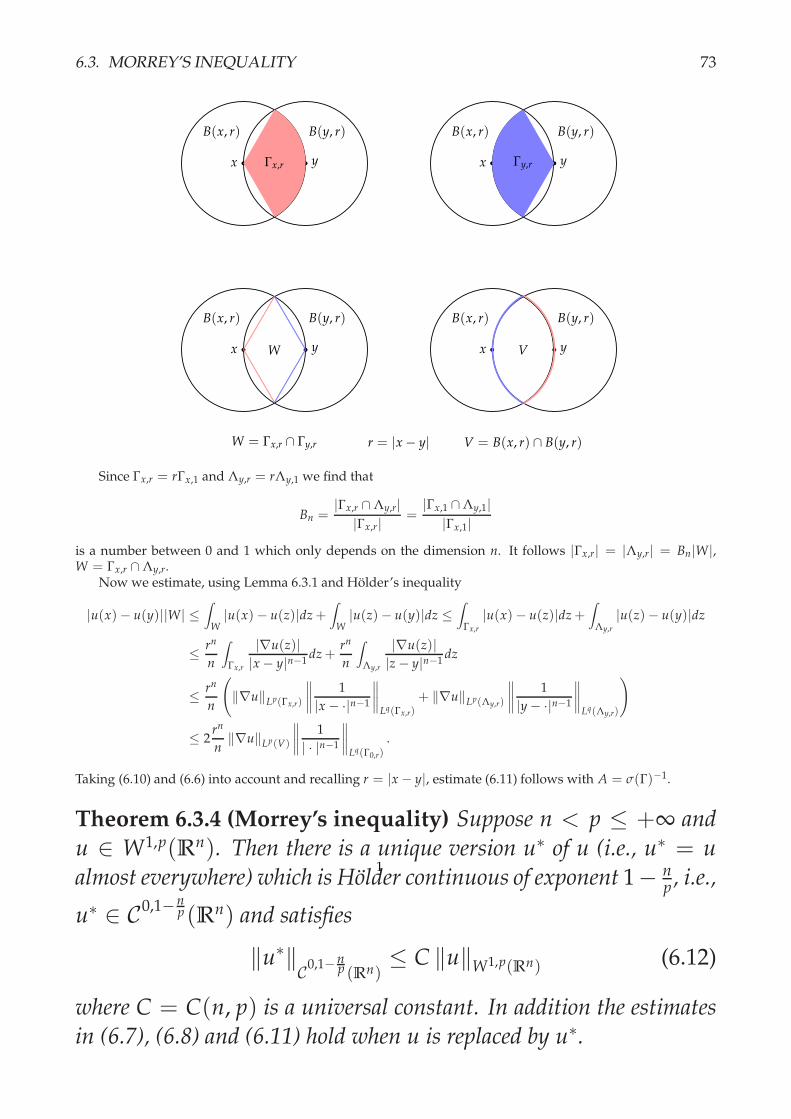
6.3. MORREY’S INEQUALITY 73

b b bbx y yxΓx,r Γy,r

B(x, r) B(y, r) B(x, r) B(y, r)

b b bbW V

B(x, r) B(y, r) B(x, r) B(y, r)

x y yx

W = Γx,r ∩ Γy,r r = |x − y| V = B(x, r) ∩ B(y, r)

1

Since Γx,r = rΓx,1 and Λy,r = rΛy,1 we find that

Bn =|Γx,r ∩ Λy,r|

|Γx,r|=

|Γx,1 ∩ Λy,1||Γx,1|

is a number between 0 and 1 which only depends on the dimension n. It follows |Γx,r| = |Λy,r| = Bn|W|,W = Γx,r ∩ Λy,r.

Now we estimate, using Lemma 6.3.1 and Hölder’s inequality

|u(x)− u(y)||W| ≤∫

W|u(x)− u(z)|dz +

∫

W|u(z)− u(y)|dz ≤

∫

Γx,r

|u(x)− u(z)|dz +∫

Λy,r

|u(z)− u(y)|dz

≤ rn

n

∫

Γx,r

|∇u(z)||x − y|n−1 dz +

rn

n

∫

Λy,r

|∇u(z)||z − y|n−1 dz

≤ rn

n

(

‖∇u‖Lp(Γx,r)

∥

∥

∥

∥

1|x − ·|n−1

∥

∥

∥

∥

Lq(Γx,r)

+ ‖∇u‖Lp(Λy,r)

∥

∥

∥

∥

1|y − ·|n−1

∥

∥

∥

∥

Lq(Λy,r)

)

≤ 2rn

n‖∇u‖Lp(V)

∥

∥

∥

∥

1| · |n−1

∥

∥

∥

∥

Lq(Γ0,r)

.

Taking (6.10) and (6.6) into account and recalling r = |x − y|, estimate (6.11) follows with A = σ(Γ)−1.

Theorem 6.3.4 (Morrey’s inequality) Suppose n < p ≤ +∞ and

u ∈ W1,p(Rn). Then there is a unique version u∗ of u (i.e., u∗ = u

almost everywhere) which is Hölder continuous of exponent 1− np , i.e.,

u∗ ∈ C0,1−np(Rn) and satisfies

‖u∗‖C0,1−n

p (Rn)≤ C ‖u‖W1,p(Rn) (6.12)

where C = C(n, p) is a universal constant. In addition the estimates

in (6.7), (6.8) and (6.11) hold when u is replaced by u∗.


Proof. At first consider the case n < p < ∞. For u ∈ C1c (R

n) Corollaries 6.3.2 and 6.3.3 imply (BC(Rn) denotesthe spaces of bounded continuous functions on Rn)

‖u‖BC(Rn) ≤ C ‖u‖W1,p(Rn) and|u(y)− u(x)||y − x|1−

np

≤ C ‖∇u‖Lp(Rn) .

This implies‖u‖

C0,1− np (Rn)

≤ C ‖u‖W1,p(Rn) . (6.13)

If u ∈ W1,p(Rn) is given, there is a sequence of functions uj ∈ C1c (R

n) such that uj → u in W1,p(Rn). Estimate

(6.13) implies that this sequence is also a Cauchy sequence in C0,1− np (Rn) and thus converges to a unique

element u∗ in this space. Clearly Estimate (6.12) holds for this limit element u∗ and u∗ = u almost everywhere.The case p = ∞ and u ∈ W1,p(Rn) can be proven via a similar approximation argument.

Corollary 6.3.5 [Morrey’s inequality] Let Ω be an open bounded sub-

set of Rn with smooth boundary (C1) and n < p ≤ ∞. Then for every

u ∈ W1,p(Ω) there exists a unique version u∗ in C0,1−np(Ω) satisfying

‖u∗‖C0,1−n

p (Ω)≤ C ‖u‖W1,p(Ω) . (6.14)

with a universal constant C = C(n, p, Ω).

Proof. Under the assumptions of the corollary there exists a continuous extension operator J : W1,p(Ω) →W1,p(Rn). Then, given u ∈ W1,p(Ω), Theorem 6.3.4 implies that there is a continuous version U∗ ∈ C0,1− n

p (Rn)of Ju which satisfies (6.12). Now define u∗ = U∗|Ω. It follows

‖u∗‖C0,1− n

p (Ω)≤ ‖U∗‖

C0,1− np (Rn)

≤ C ‖Ju‖W1,p(Rn) ≤ C ‖u‖W1,p(Ω) .

6.4 Gagliardo-Nirenberg-Sobolev inequality

This very important inequality is of the form

‖u‖Lq ≤ C ‖∇u‖Lp , u ∈ C1c (R

n) (6.15)

for a suitable exponent q for a given exponent p, 1 ≤ p ≤ n.This exponent is easily determined through the scale covarianceof the quantities in this inequality. For λ > 0 introduce uλ bysetting uλ(x) = u(λx). A simple calculation shows ‖uλ‖Lq =λ−n/q ‖u‖Lq and ‖∇uλ‖Lp = λ1−n/p ‖∇u‖Lp. Thus inserting uλ

into (6.15 gives

λ−n/q ‖u‖Lq ≤ Cλ1−n/p ‖∇u‖Lp

6.4. GAGLIARDO-NIRENBERG-SOBOLEV INEQUALITY 75

for all λ > 0. This is possible for all u ∈ C1c (R

n) only if

1 − n/p + n/q = 0, i.e.,1p=

1n+

1q

. (6.16)

It is a standard notation to denote the exponent q which solves(6.16) by p∗, i.e.,

p∗ =np

n − p

with the understanding that p∗ = ∞ if p = n.Since the case 1 < p < n can easily be reduced to the case p =

1, we have to prove this inequality for p = 1, i.e., p∗ = 1∗ = nn−1 .

Theorem 6.4.1 For all u ∈ W1,1(Rn) one has

‖u‖1∗ = ‖u‖ nn−1

≤n

∏i=1

(

∫

Rn|∂iu(x)|dx

)1n

≤ n−12 ‖∇u‖1 (6.17)

Proof. According to Theorem 6.2.2 every element u ∈ W1,1(Rn) is the limit of a sequence of elements uj ∈C1

c (Rn). Hence is suffices to prove this inequality for u ∈ C1

c (Rn), and this is done by induction on the dimen-

sion n.We suggest that the reader proves the GNS inequality for n = 1 and n = 2. Here we present first the case

n = 3 before we come to the general case.Suppose that u ∈ C1

c (R3) is given. Observe that now 1∗ = 3/2. Introduce the notation x1 = (y1, x2, x3),

x2 = (x1, y2, x3), and x3 = (x1, x2, y3). The fundamental theorem of calculus implies for i = 1, 2, 3

|u(x)| ≤∫ xi

−∞|∂iu(xi)|dyi ≤

∫ ∞

−∞|∂iu(xi)|dyi,

hence multiplication of these three inequalities gives

|u(x)| 32 ≤

3

∏i=1

(

∫ ∞

−∞|∂iu(xi)|dyi

) 12

.

Now integrate this inequality with respect to x1 and note that the first factor on the right does not depend onx1:

∫

R

|u(x)| 32 dx1 ≤

(

∫ ∞

−∞|∂1u(x1)|dy1

)12∫

R

3

∏i=2

(

∫ ∞

−∞|∂iu(xi)|dyi

)12

dx1

Apply Hölder’s inequality (for p = q = 2) to the second integral, this gives the estimate

≤(

∫ ∞

−∞|∂1u(x)|dx1

)12 3

∏i=2

(

∫ ∞

−∞|∂iu(xi)|dx1dyi

)12

.

Next we integrate this inequality with respect to x2 and apply again Hölder’s inequality to get

∫

R2|u(x)| 3

2 dx1dx2 ≤(

∫

R2|∂2u(x)dx1dx2

)12∫

R

(

∫ ∞

−∞|∂1u(x1)|dx1

)12(

∫ ∞

−∞|∂3u(x3)|dx1dy3

)12

dx2

≤(

∫

R2|∂2u(x)dx1dx2

) 12(

∫

R2|∂1u(x1)|dx1dx2

) 12(

∫

R3|∂3u(x)|dx1dx2dx3

) 12


A final integration with respect to x3 and applying Hölder’s inequality as above implies

∫

R3|u(x)| 3

2 dx1dx2dx3 ≤3

∏i=1

(

∫

R3|∂iu(x)|dx1dx2dx3

)12≤(

∫

R3|∇u(x)|dx1dx2dx3

)12

which is the GNS inequality for n = 3.The general case uses the same strategy. Naturally some more steps are necessary. Now we have 1∗ = n

n−1 .For x = (x1, . . . , xn) ∈ Rn introduce the variables xi = (x1, . . . , xi−1, yi, xi+1, . . . , xn). The fundamental theoremof calculus implies for i = 1, . . . , n

|u(x)| ≤∫

R

|∂iu(xi)|dyi

and thus

|u(x)| nn−1 ≤

n

∏i=1

(

∫

R

|∂iu(xi)|dyi

)1

n−1. (6.18)

Recall Hölder’s inequality for the product of n − 1 functions in the form∥

∥

∥

∥

∥

n

∏i=2

fi

∥

∥

∥

∥

∥

1

≤n

∏i=2

‖ fi‖n−1 (6.19)

and integrate (6.18) with respect to x1 to get

∫

R

|u(x)| nn−1 dx1 ≤

(

∫

R

|∂1u(x)|dx1

) 1n−1

∫

R

n

∏i=2

(

∫

R

|∂iu(xi)|dyi

) 1n−1

dx1

≤(

∫

R

|∂1u(x)|dx1

) 1n−1 n

∏i=2

(

∫

R2|∂iu(xi)|dx1dyi

) 1n−1

≤(

∫

R

|∂1u(x)|dx1

)1

n−1(

∫

R2|∂2u(x)|dx1dx2

)1

n−1 n

∏i=3

(

∫

R2|∂iu(xi)|dx1dyi

)1

n−1

Now integrate this inequality with respect to x2 and apply (6.19) again. This implies

∫

R

|u(x)| nn−1 dx1dx2 ≤

(

∫

R2|∂2u(x)|dx1dx2

)1

n−1∫

R

(

∫

R

|∂1u(x)|dx1

)1

n−1 n

∏i=3

(

∫

R2|∂iu(xi)|dx1dyi

)1

n−1dx2

≤(

∫

R2|∂2u(x)|dx1dx2

)1

n−1(

∫

R2|∂1u(x)|dx1dx2

)1

n−1 n

∏i=3

(

∫

R3|∂iu(xi)|dx1dx2dyi

)1

n−1.

Obviously one can repeat these steps successively for x3, . . . , xn and one proves by induction that for k ∈1, . . . , n we get the estimate

∫

Rk|u(x)| n

n−1 dx1dx2 · · · dxk ≤k

∏i=1

(

∫

Rk|∂iu(x)|dx1dx2 · · · dxk

)n

n−1

×n

∏i=k+1

(

∫

Rk+1|∂iu(x)|dx1dx2 · · · dxkdyi

)n

n−1

where naturally for k = n the second product does not occur. Thus for k = n one has∫

Rn|u(x)| n

n−1 dx1dx2 · · · dxn ≤n

∏i=1

(

∫

Rn|∂iu(x)|dx1dx2 · · · dxn

)n

n−1

≤n

∏i=1

(

∫

Rn|∇u(x)|dx

) nn−1

. (6.20)

In order to improve this estimate recall Young’s inequality in the elementary form ∏ni=1 Ai ≤ 1

n ∑ni=1 An

i , whereAi ≥ 0. Thus we get

‖u‖ nn−1

≤n

∏i=1

(

∫

Rn|∂iu(x)|dx

)1n

≤ 1n

n

∑i=1

∫

Rn|∂iu(x)|dx

and by Hölder’s inequality one knows ∑ni=1 |∂iu(x)| ≤ √

n |∇u(x)|, hence ‖u‖ nn−1

≤ 1√n‖∇u‖1.


Remark 6.4.2 The starting point of our estimates was the identity

u(x) =∫ xi

−∞∂iu(xi)dyi and the resulting estimate

|u(x)| ≤∫

R

|∂iu(xi)|dyi, i = 1, . . . , n.

If we write

u(x) =12

(

∫ xi

−∞

∂iu(xi)dyi −∫ ∞

xi

∂iu(xi)dyi

)

,

we can improve this estimate to

|u(x)| ≤ 12

∫

R

|∂iu(xi)|dyi, i = 1, . . . , n.

Next we look at the case 1 < p < n. As we will see it can easilybe reduced to the case p = 1.

Theorem 6.4.3 If 1 ≤ p < n then, for all u ∈ W1,p(Rn), with

p∗ = npn−p ,

‖u‖p∗ ≤1√n

p(n − 1)n − p

‖∇u‖p . (6.21)

Proof. Since elements in W1,p(Rn) can be approximated by elements in C1c (R

n) it suffices to prove Estimate(6.21) for u ∈ C1

c (Rn). For such a function u consider the function v = |u|s ∈ C1

c (Rn) for an exponent s > 1 to

be determined later. We have ∇v = s|u|s−1sgn(u)∇u and thus by applying (6.17) to v we get

‖|u|s‖1∗ ≤1√n‖∇|u|s‖1 =

s√n

∥

∥

∥|u|s−1∇u

∥

∥

∥

1≤ s√

n

∥

∥

∥|u|s−1

∥

∥

∥

q‖∇u‖p (6.22)

where q is the Hölder conjugate exponent of p. Note that this estimate can be written as

‖u‖ss1∗ ≤

s√n‖u‖s−1

(s−1)q ‖∇u‖p .

Now choose s such that s1∗ = (s − 1)q. This gives s = qq−1∗ = p∗

1∗ and accordingly the last estimate can bewritten as

‖u‖sp∗ ≤

s√n‖u‖s−1

p∗ ‖∇u‖p .

Inserting the value s = p(n−1n−p of s now yields (6.21).

Corollary 6.4.4 Suppose that Ω ⊂ Rn is a bounded open set with C1-

boundary. Then for all p ∈ [1, n) and 1 ≤ q ≤ p∗ there is a constant

C = C(Ω, p, q) such that for all u ∈ W1,p(Ω)

‖u‖q ≤ C ‖u‖1,p .


Proof. Under the given conditions on Ω one can show that every u ∈ W1,p(Ω) has an extension to Ju ∈W1,p(Rn) (i.e., Ju|Ω = u and J : W1,p(Ω) → W1,p(Rn) is continuous). Then for u ∈ C1(Ω) ∩ W1,p(Ω)

‖u‖Lp∗ (Ω) ≤ C ‖Ju‖Lp∗ (Rn) ≤ C ‖∇(Ju)‖Lp(Rn) ≤ C ‖u‖W1,p(Ω) . (6.23)

Since C1(Ω) is dense in W1,p(Ω), this estimate holds for all u ∈ W1,p(Ω). If now 1 ≤ q < p∗ a simpleapplication of Hölder’s inequality gives

‖u‖Lq(Ω) ≤ ‖u‖Lp∗ (Ω) ‖1‖Ls(Ω) = ‖u‖Lp∗ (Ω) |Ω|1/s ≤ C|Ω|1/s ‖u‖W1,p(Ω)

where 1s +

1p∗ = 1

q .

6.4.1 Continuous Embeddings of Sobolev spaces

In this short review of the classical theory of Sobolev spaces wecan only discuss the main embeddings results. In the literatureone finds many additional cases.

For convenience of notation let us introduce, for a given num-ber r ≥ 0,

r+ =

r if r /∈ N0

r + δ if r ∈ N0

where δ > 0 is some arbitrary small number.

Lemma 6.4.5 For i ∈ N and p ≥ n and i > n/p (i.e., i ≥ 1 if p > n

and i ≥ 2 if p = n) one has

W i,p(Ω) → C i−(n/p)+(Ω)

and there is a constant C > 0 such that for all u ∈ W i,p(Ω)

‖u‖C i−(n/p)+(Ω)≤ C ‖u‖i,p (6.24)

Proof. For a number r = k + α with k ∈ N0 and 0 ≤ α < 1 we write Cr(Ω) for Ck,α. As earlier it suffices toprove (6.24) for u ∈ C∞(Ω). For such u and p > n and |α| ≤ i − 1 apply Morrey’s inequality to get

‖Dαu‖C0,1−n/p(Ω) ≤ C ‖Dαu‖i,p

and therefore with C i−n/p(Ω) ≡ C i−1,1−n/p(Ω), we get (6.24).If p = n (and thus i ≥ 2) choose q ∈ (1, n) close to n so that i > n/q and q∗ = qn

n−q > n. Then, by the firstpart of Theorem (6.4.6) and what we have just shown

W i,n(Ω) → W i,q(Ω) → W i−1,q∗(Ω) → C i−2,1−n/q∗(Ω).

As q ↑ n implies n/q∗ ↓ 0, we conclude W i,n(Ω) → C i−2,α(Ω) for any α ∈ (0, 1) which is written as

W i,n(Ω) → C i−(n/n)+(Ω).


Theorem 6.4.6 (Sobolev Embedding Theorems) Assume that Ω =Rn or that Ω is a bounded open subset of Rn with a C1-boundary; fur-

thermore assume that 1 ≤ p < ∞ and k, m ∈ N with m ≤ k. Then

one has:

(1) If p < n/m, then Wk,p(Ω) → Wk−m,q(Ω) for q = npn−pm or

1q = 1

p − mn > 0, and there is a constant C > 0 such that

‖u‖k−m,q ≤ C ‖u‖k,p for all u ∈ Wk,p(Ω). (6.25)

(2) If p > n/k, then Wk,p(Ω) → Ck−(n/p)+(Ω) and there is a con-

stant C > 0 such that

‖u‖Ck−(n/p)+(Ω)≤ C ‖u‖k,p for all u ∈ Wk,p(Ω). (6.26)

Proof. Suppose p < n/m and u ∈ Wk,p(Ω); then Dαu ∈ W1,p(Ω) for all |α| ≤ k − 1. Corollary 6.4.4 impliesDαu ∈ Lp∗(Ω) for all |α| ≤ k − 1 and therefore Wk,p(Ω) → Wk−1,p∗(Ω) and there is a constant C1 > 0 suchthat

‖u‖k−1,p1≤ C1 ‖u‖k,p (6.27)

for all u ∈ Wk,p(Ω), with p1 = p∗. Next define pj, j ≥ 2, inductively by pj = p∗j−1. Thus 1p j

= 1p j−1

− 1n

and since p < n/m we have 1pm

= 1p − m

n > 0. Therefore we can (6.27 repeatedly and find that the followinginclusion maps are all bounded:

Wk,p(Ω) → Wk−1,p1(Ω) → Wk−2,p2(Ω) · · · → Wk−m,pm(Ω)

and part (1) follows.In order to prove part (2) consider p > n/k. For p ≥ n the statement follows from Lemma 6.4.5. Now

consider the case n > p > n/k and choose the largest m such that 1 ≤ m < k and n/m > p. Define q ≥ n byq = np

n−mp (i.e., 1q = 1

p − mn > 0). Then, by what we have established above, the following inclusion maps are

all bounded:

Wk,p(Ω) → Wk−m,q(Ω) → Ck−m−(n/q)+(Ω) = Ck−m−( np−m)+(Ω) = Ck−(n/p)+(Ω)

which is the estimate of Part (2).

In the case p = 2 and Ω = Rn one has the Fourier transformF available as a unitary operator on L2(Rn). This allows to givea convenient characterization of the Sobolev space Hk(Rn) =Wk,2(Rn) and to prove a useful embedding result.

Recall that for u ∈ Hk(Rn) one has F (Dαu)(p) = i|α|pαF (u)(p).Hence we can characterize this space as

Hk(Rn) =

u ∈ L2(Rn) : pαF (u) ∈ L2(Rn), |α| ≤ k

=

u ∈ L2(Rn) : (1 + p2)k/2F (u) ∈ L2(Rn)

.


This definition can be extended to arbitrary s ∈ R and thus wecan introduce the spaces

Hs(Rn) =

u ∈ L2(Rn) : (1 + p2)s/2F (u) ∈ L2(Rn)

.

As we are going to show this space can be continuously embed-ded into the space

Ckb(R

n) =

f ∈ Ck(Rn) : ‖ f ‖k,∞ = sup|α|≤k

supx∈Rn

|Dα f (x)| < ∞

.

Theorem 6.4.7 For k ∈ N and s > k + n/2 the Sobolev space

Hs(Rn) is continuously embedded into the space Ckb(R

n) and one has

for all u ∈ Hs(Rn)

‖u‖k,∞ ≤ C ‖u‖s,2 , lim|x|→∞

|Dαu(x)| = 0, |α| ≤ k.

Proof. Recall that the Lemma of Riemann-Lebesgue says that the Fourier transform of an L1(Rn) function iscontinuous and vanishes at infinity. For |α| ≤ k and s > k + n/2 one knows

∫

Rn

|p2α|(1 + p2)s

dp = C2α < ∞.

Thus, for u ∈ Hs(Rn) we can estimate

∫

Rn|pα(Fu)(p)|dp ≤ Cα

(

∫

Rn(1 + p2)s|Fu(p)|2dp

)1/2

= Cα ‖u‖s,2

and therefore for all x ∈ Rn

|Dαu(x)| = |∫

Rneipx pα(Fu)(p)dp| ≤ Cα ‖u‖s,2 .

It follows ‖u‖k,∞ ≤ ‖u‖s,2. By applying the Lemma of Riemann-Lebesgue we conclude.

6.4.2 Compact Embeddings of Sobolev spaces

Here we show that some of the continuous embeddings estab-lished above are actually compact, that is they map boundedsubsets into precompact sets. There are various ways to provethese compactness results. We present a proof which is basedon the characterization of compact subsets M ⊂ Lq(Rn), due toKolmogorov and Riesz [Kol31, Rie33].


Theorem 6.4.8 (Kolmogorov-Riesz compactness criterion) Suppose

1 ≤ q < ∞. Then a subset M ⊂ Lq(Rn) is precompact if, and only if

M satisfies the following threes conditions:

(a) M is bounded, i.e.,

∃C<∞ ∀ f∈M ‖ f ‖ ≤ C;

(b)

∀ǫ>0 ∃R<∞ ∀ f∈M

∥

∥π⊥R f∥

∥

q< ǫ;

(c)

∀ǫ>0 ∃r>0 ∀ f∈M ∀y∈Rn

|y|<r

∥

∥τy( f )− f∥

∥

q< ǫ.

Here the following notation is used: π⊥R is the operator of multi-

plication with the characteristic function of the set x ∈ Rn : |x| > Rand τy denotes the operator of translation by y ∈ Rn, i.e., τy( f )(x) =f (x + y).

Remark 6.4.9 If Ω ⊂ Rn is an open bounded subset we can consider

Lq(Ω) as a subset of Lq(Rn) by extending all elements f ∈ Lq(Ω)by 0 to all of Rn. Then the above characterization provides also a

characterization of precompact subset M ⊂ Lq(Ω) where naturally

condition (b) is satisfied always and where in condition (c) we have to

use these extensions.

There are several versions of compact embedding results de-pending on the assumptions on the domain Ω ⊂ Rn whichare used. The following version is already quite comprehensivethough there are several newer results of this type.

Theorem 6.4.10 (Rellich-Kondrachov compactness theorem) Let

Ω ⊂ Rn be a bounded domain. Assume that the boundary of Ω is suf-

ficiently smooth and that 1 ≤ p < ∞ and k = 1, 2, . . .. Then the

following holds:

(a) The following embeddings are compact:


(i) kp < n: Wk,p(Ω) → Lq(Ω), 1 ≤ q < p∗ = npn−kp ;

(ii) kp = n: Wk,p(Ω) → Lq(Ω), 1 ≤ q < ∞;

(iii) kp > n: Wk,p(Ω) → C0b(Ω).

(b) For the subspaces Wk,p0 (Ω) the embeddings (i) - (iii) are compact

for arbitrary open sets Ω.

Proof. Because of time constraints we discuss here only the proof of embedding (i) of part (a) for k = 1.According to Corollary 6.4.4 the inclusion mapping Wk,p(Ω) → Lq(Ω) is continuous for 1 ≤ q ≤ p∗. We haveto show that every bounded subset M ⊂ Wk,p(Ω) is precompact in Lq(Ω) for 1 ≤ q < p∗. This is done bythe Kolmogorov-Riesz compactness criterion. By Remark 6.4.9 only conditions (a) and (c) have to be verifiedfor M considered as a subset of Lq(Ω). Since we know that this inclusion map is continuous, it follows that Mis bounded in Lq(Ω) too and thus Condition (a) of the Kolmogorov-Riesz criterion is verified and we are leftwith verifying Condition (c).

Observe that for 1 ≤ q < p∗ Hölder’s inequality implies

‖u‖q ≤ ‖u‖α1 ‖u‖1−α

p∗ , α =1q

p∗ − q

p∗ − 1∈ (0, 1).

Now let M ⊂ W1,p(Ω) be bounded; then this set is bounded in Lp∗(Ω) and hence there is a constant C < ∞

such that for all u ∈ M we have‖u‖q ≤ C ‖u‖α

1

and it follows∥

∥τyu − u∥

∥

q≤ 2C

∥

∥τyu − u∥

∥

α1 , ∀ u ∈ M. (6.28)

Therefore it suffices to verify condition (c) of Theorem 6.4.8 for the norm ‖·‖1. For i = 1, 2, . . . introduce thesets

Ωi = x ∈ Ω : d(x, ∂Ω) > 2/i ,

where d(x, ∂Ω) denotes the distance of the point x from the boundary ∂Ω of Ω. Another application of Hölder’sinequality gives, for all u ∈ M,

∫

Ω\Ωi

|u(x)|dx ≤(

∫

Ω\Ωi

|u(x)|p∗dx

)1/p∗ (∫

Ω\Ωi

dx

)1− 1p∗

≤ ‖u‖p∗ |Ω\Ωi|1− 1

p∗ ≤ CM|Ω\Ωi|1− 1

p∗

where CM is a bound for M in Lp∗(Ω). Given ǫ > 0 we can therefore find i0 = i0(ǫ) such that∫

Ω\Ωi

|u(x)|dx < ǫ/4

holds for all u ∈ M. Extend u ∈ M outside Ω by 0 to get

u(x) =

u(x), x ∈ Ω,0, otherwise.

For a fixed i ≥ i0 and y ∈ Rn, |y| < 1/i, we estimate

∥

∥τyu − u∥

∥

1 =∫

Ωi

|u(x + y)− u(x)|dx +∫

Ω\Ωi

|u(x + y)− u(x)|dx

≤∫

Ωi

|u(x + y)− u(x)|dx + ǫ/2


And the integral is estimated as follows:

=∫

Ωi

|∫ 1

0

d

dtu(x + ty)dt|dx =

∫

Ωi

|∫ 1

0y · ∇u(x + ty)dt|dx ≤ |y|

∫

Ω2i

|∇u(x)|dx

≤ |y||Ω2i|1p′ ‖∇u‖Lp(Ω2i)

≤ |y||Ω2i|1p′ C ≤ |y||Ω|

1p′ C

It follows that there is r0 > 0 such that∥

∥τyu − u∥

∥

1 < ǫ for all |y| < r0. By estimate (6.28) we conclude thatCondition (c) of Theorem 6.4.8 holds and therefore by this theorem M ⊂ W1,p(Ω) is precompact in Lq(Ω).

Remark 6.4.11 The general case of Wk,p(Ω) with k > 1 follows from

the following observation which can be proven similarly.

For m ≥ 1 and 1q >

1p − m

n > 0 the inclusion of Wk,p(Ω) into

Wk−m,q(Ω) is compact.

In the proof of compactness of the Sobolev embeddings thefact that the underlying set Ω ⊂ R

n is bounded entered in an im-portant way. We now mention a result for the pre-compactnessin Lq(Rn) of certain bounded sets M ⊂ W1,p(Rn).

Theorem 6.4.12 Let M ⊂ W1,p(Rn) be bounded and suppose that

∀ǫ>0 ∃R<∞ ∀u∈M

∥

∥π⊥R u∥

∥

1,p < ǫ (6.29)

holds. Then M is pre-compact in Lq(Rn) provided

n

p− 1 <

n

q≤ n

p.


Chapter 7

Some Applications

7.1 Spectral Theory for compact Operators

This chapter serves to illustrate how the variational methodscan be used in a variety of mathematical problems. Naturally,in this introduction on we only consider those which are typicaland technically not too involved. We begin with two classical re-sults. Then we proceed to solve partial differential equations byvariational methods. Here we distinguish between linear andnonlinear problems and between those which are defined overbounded and unbounded domains Ω ⊂ Rn.

Theorem 7.1.1 (Spectral Theorem for compact self-adjoint Ops.)

Let H be a separable Hilbert space and A 6= 0 a compact self-adjoint

operator on H. Then there are an orthonormal system ej : j ∈ Nof eigenvectors and a system of real eigenvalues λj : j ∈ N, i.e.,

Aej = λjej, with the following properties.

a) The eigenvalues are arranged in descending order of magnitude,

i.e., |λ1| ≥ · · · |λj| ≥ |λj+1| ≥ · · · .

b) Either finitely many of the eigenvalues are nonzero, or all eigen-

values are nonzero, and limj→∞ λj = 0, i.e., 0 is the only cluster

point of the eigenvalues.

c) The multiplicity of each nonzero eigenvalues is finite:

dim ker(A − λjI) < ∞ for all j ∈ N.

85

86 CHAPTER 7. SOME APPLICATIONS

d) The orthonormal system of eigenvectors ej : j ∈ N is complete

if, and only if, A is injective.

Proof. Naturally we discuss here only the ‘variational part’ of the proof. In a first step we collect some basicfacts about operators on Hilbert spaces. Recall that a compact operator in a separable Hilbert space H is char-acterized by the property that, for every weakly convergent sequence (xn)n∈N in H, the sequence of images(Axn)n∈N converges strongly. This fact implies immediately that the functions

x → ‖Ax‖ and x → 〈x, Ax〉

are weakly continuous on H.Recall furthermore that the norm of an operator A can be calculated as follows:

‖A‖ = supu∈B1(H)

‖Au‖ = supu∈S1(H)

‖Au‖ = ‖A‖B(H) ,

B1(H) = x ∈ H : ‖x‖ ≤ 1, S1(H) = x ∈ H : ‖x‖ = 1.

In the second step we determine the largest (in absolute value) eigenvalue of A. Since the closed unit ballB1(H) of a Hilbert space is weakly (sequentially) compact and the functions u → ‖Au‖ and u → |〈u, Au〉| areweakly continuous, Theorem 2.3.4 can be applied. Hence there is e1 ∈ B1(H) such that

‖Ae1‖ = supu∈B1(H)

‖Au‖ = ‖A‖ .

A 6= 0 implies e1 6= 0, and so ‖e1‖ = 1, since if 0 < ‖e1‖ < 1 then

‖Ae1‖ <‖Ae1‖‖e1‖

= ‖Ae1‖ ,

a contradiction to e1 = 1‖e1‖ e1 ∈ S1(H).

In the third step it is shown that the maximizing element e1 ∈ S1(H) is an eigenvalue of A. To this endwe note that the function x → Q(x) = 〈x, Ax〉 is differentiable on H with the Fréchet derivative Q′(x)(h) =2〈Ax, h〉 for all h ∈ H (here we use self-adjointness A∗ = A of A) and, as we had mentioned above,

supx∈S1(H)

Q(x) = ±‖A‖ .

The constraint φ(x) = 〈x, x〉 − 1 = 0 is defined by a mapping φ which is regular at all points of the level surfaceφ−1(0) = S1(H), since φ′(x)(h) = 2〈x, h〉 for all h ∈ H.

Since we know that e1 ∈ φ−1(0) is an extremal point of the functional Q, Theorem 4.3.1 (existence of aLagrange multiplier) assures that there is λ1 ∈ R such that

Q′(e1) = λ1φ′(e1).

It follows Ae1 = λ1e1 and |λ1| = ‖A‖.In a fourth step a reduction of the problem to a ‘smaller’ space H1 = e1⊥ ⊂ H is done. Since A is

self-adjoint, it maps the space H1 into itself. Thus the restriction A1 = A H1 of A to the subspace H1 iswell defined. It also is self-adjoint and compact. Its norm is not larger than that of A: ‖A1‖B(H1)

≤ ‖A‖B(H).If A1 6= 0, then our considerations from above apply to the compact self-adjoint operator A1 in the reducedHilbert space H1. Hence there are a normalized eigenvector e2 ∈ H1 of A1 for an eigenvalue λ2, such that

|λ2| = ‖A1‖B(H1)≤ ‖A‖B(H) = |λ1| and 〈e2, e1〉 = 0

hold. This reduction can be iterated and produces a sequence of subspaces Hj =

ej−1⊥ ⊂ Hj−1 and oper-

ators Aj = A Hj. Obviously this iteration stops for j when Aj = 0; otherwise it continues. The rest of theproof does not use anymore variational arguments is omitted.

The above result establishes the existence and some of the prop-erties of eigenvalues of a compact self-adjoint operator. The

7.1. SPECTRAL THEORY FOR COMPACT OPERATORS 87

question arises whether there is some method to calculate theseeigenvalues. And indeed such a method has been worked outlong ago and is known as the classical minimax principle of Courant–

Weyl–Fischer–Poincaré–Rayleigh–Ritz.

Theorem 7.1.2 (Minimax Principle) Let H be a real separable Hilbert

space and A ≥ 0 a self-adjoint operator on H with spectrum σ(A) =λm : m ∈ N ordered according to size, λm ≤ λm+1. For m =1, 2, . . . denote by Em the family of all m-dimensional subspaces Em

of H. Then the eigenvalue λm can be calculated as

λm = minEm∈Em

maxv∈Em

〈v, Av〉〈v, v〉 . (7.1)

Proof. The proof is obtained by determining the lower bound for the values of the Rayleigh quotient R(v) =〈v,Av〉〈v,v〉 . In order to do this we expand every v ∈ H in terms of eigenvectors ej of A. This gives v = ∑

∞i=1 aiei and

〈v, v〉 = ∑∞i=1 a2

i . In this form the Rayleigh quotient reads

R(v) =∑

∞i=1 λia

2i

∑∞i=1 a2

i

.

Denote by Vm the linear subspace generated by the first m eigenvectors of A. It follows that

maxv∈Vm

R(v) = max(a1,...,am)∈Rm

∑mi=1 λia

2i

∑mi=1 a2

i

= λm = R(em),

and thus we are left with showing maxv∈Em R(v) ≥ λm for every other subspace Em ∈ Em. Let Em 6= Vm besuch a subspace; then Em ∩ V⊥

m 6= 0 and therefore

maxv∈Em

R(v) ≥ maxv∈Em∩V⊥

m

R(v).

Every v ∈ Em ∩ V⊥m is of the form v = ∑i≥m+1 aiei and for such vectors we have

R(v) =∑i≥m+1 λia

2i

∑i≥m+1 a2i

≥ λm+1 ≥ λm.

This then completes the proof.

Theorem 7.1.2 implies for the smallest eigenvalue of the oper-ator A the simple formula

λ1 = minv∈E, v 6=0

〈v, Av〉〈v, v〉 . (7.2)


7.2 Some linear boundary and eigenvalue problems

7.2.1 The Dirichlet–Laplace operator

The goal of this section is to illustrate the application of the gen-eral strategy and the results developed thus far. This is doneby solving several relatively simple linear boundary and eigen-value problems. The typical example is the Laplace operatorwith Dirichlet boundary conditions on a bounded domain Ω.Naturally, for these concrete problems we have to use concretefunction spaces, and we need to know a number of basic factsabout them. In this brief introduction we have to refer the readerto the literature for the proof of these facts. We recommend thebooks [LL01, JLJ98, BB92].

For a bounded domain Ω ⊂ Rn with smooth boundary ∂Ω

consider the real Hilbert space L2(Ω) with inner product 〈·, ·〉2.Then define a space H1(Ω) as

H1(Ω) =

u ∈ L2(Ω) : ∂ju ∈ L2(Ω), j = 1, . . . , n

. (7.3)

Here naturally the partial derivatives ∂ju are understood in theweak (distributional) sense. One shows that H1(Ω) is a Hilbertspace with the inner product

〈u, v〉 = 〈u, v〉2 + 〈Du, Dv〉2 ∀ u, v ∈ H1(Ω) (7.4)

where Du = (∂1u, . . . , ∂nu) and where in the second term thenatural inner product of L2(Ω)×n is used. This space is theSobolev space W1,2(Ω) as introduced in Chapter 6. Next define asubspace H1

0(Ω) of this space as the closure of the space D(Ω)of C∞-functions on Ω with compact support:

H10(Ω) = closure of D(Ω) in H1(Ω). (7.5)

Intuitively, H10(Ω) is the subspace of those u ∈ H1(Ω) whose

restriction to the boundary ∂Ω vanishes, u|∂Ω = 0.

7.2. SOME LINEAR BOUNDARY AND EIGENVALUE PROBLEMS 89

The Sobolev space H1(Ω) is by definition contained in theHilbert space L2(Ω), however for us of much greater impor-tance is the fact that the following embeddings for 2 ≤ n,

H1(Ω) → Lq(Ω), 1 ≤ q < 2∗ =2n

n − 2, 2 < n (7.6)

andH1(Ω) → Lq(Ω), 1 ≤ q < ∞, 2 = n (7.7)

are compact (see Theorem 6.4.10). This means that every weaklyconvergent sequence in H1(Ω) converges strongly in Lq(Ω). Inaddition we are going to use the important Sobolev inequality

‖u‖q ≤ S ‖Du‖p = S(n

∑j=1

∥

∥∂ju∥

∥

p

p)1/p ∀ u ∈ H1(Ω), (7.8)

where S is the Sobolev constant depending on q, n and whereq is in the range indicated in (7.6) respectively (7.7) (compareCorollary 6.4.4) .

Now we are in the position to show that the famous Dirichletproblem has a solution.

Theorem 7.2.1 (Dirichlet problem) Let Ω ⊂ Rn be a bounded open

set with smooth boundary and v0 ∈ H1(Ω) some given element. Then

the Dirichlet integral

f (v) =∫

Ω

|Dv(x)|2dx =∫

Ω

n

∑j=1

|∂jv(x)|2dx (7.9)

is minimized on M = v0 + H10(Ω) by an element v ∈ M satisfying

v = 0 in Ω and v|∂Ω = v0|∂Ω. (7.10)

Proof. Observe that f (u) = Q(u, u) with the quadratic functional Q(u, v) = 〈Du, Dv〉2. This quadratic formsatisfies, because of inequality (7.8), the estimate

c ‖u‖2 ≤ Q(u, u) ≤ ‖u‖2

for some c > 0. It follows that Q is a strictly positive continuous quadratic form on H1(Ω) and thus f is astrictly convex continuous function on this space (see the proof of Theorem 2.4.1). We conclude, by Lemma2.3.2 or Theorem 2.4.1, that f is weakly lower semi-continuous on H1(Ω).


As a Hilbert space, H10(Ω) is weakly complete and thus the set M = v0 + H1

0(Ω) is weakly closed. There-fore Theorem 2.3.5 applies and we conclude that there is a minimizing element v for the functional f on M.

Since the minimizing element v = v0 + u ∈ M satisfies f (v) = f (v0 + u) ≤ f (v0 + w) for all w ∈ H10(Ω)

we deduce as earlier that f ′(v)(w) = 0 for all w ∈ H10(Ω) and thus

0 = f ′(v)(w) =∫

ΩDv(x) · Dw(x)dx ∀w ∈ D(Ω).

Recalling the definition of differentiation in the sense of distributions, this means −v = 0 in the sense ofD′(Ω). Now the Lemma of Weyl (see [JLJ98, BB92]) implies that −v = 0 also holds in the classical sense, i.e.,as an identity for functions of class C2.

Because for u ∈ H10(Ω) one has u|∂Ω = 0 the minimizer v satisfies the boundary condition too. Thus we

conclude.

As a simple application of the theory of constrained mini-mization we solve the eigenvalue problem for the Laplace op-erator on an open bounded domain Ω with Dirichlet boundaryconditions, i.e., the problem is to find a number λ and a functionu 6= 0 satisfying

−u = λu in Ω, u|∂Ω = 0. (7.11)

The strategy is simple. On the Hilbert space H10(Ω) we min-

imize the functional f (u) = 12〈Du, Du〉2 under the constraint

g(u) = 12 for the constraint functional g(u) = 1

2〈u, u〉2. Thederivative of g is easily calculated; it is g′(u)(v) = 〈u, v〉2 forall v ∈ H1

0(Ω) and thus the level surface [g = 12] consists only of

regular points of the mapping g.Since we know that f is weakly lower semi-continuous and

coercive on H10(Ω) we can prove the existence of a minimizer for

the functional f on [g = 12] by verifying that [g = 1

2] is weaklyclosed and then to apply Theorem 2.3.5.

Suppose a sequence (uj)j∈N converges to u weakly in H10(Ω).

According to the Sobolev embedding (7.6) the space H10(Ω) is

compactly embedded into the space L2(Ω) and thus this se-quence converges strongly in L2(Ω) to u. It follows that g(uj) →g(u) as j → ∞, i.e., g is weakly continuous on H1

0(Ω) and itslevel surfaces are weakly closed.

Theorem 2.3.5 implies the existence of a minimizer of f un-der the constraint g(u) = 1/2. Using Corollary 4.2.3 and Theo-rem 4.3.1 we deduce that there is a Lagrange multiplier λ ∈ R

7.2. SOME LINEAR BOUNDARY AND EIGENVALUE PROBLEMS 91

for this constrained minimization problem, i.e., a real number λ

satisfying f ′(u) = λg′(u). In detail this identity reads∫

Ω

Du(x) · Dv(x)dx = λ∫

Ω

u(x)v(x)dx ∀ v ∈ H10(Ω),

and in particular for all v ∈ D(Ω), thus −u = λu in D′(Ω);and by elliptic regularity theory (see for instance Section 9.3of [BB92]) we conclude that this identity holds in the classicalsense. Since the solution u belongs to the space H1

0(Ω) it satis-fies the boundary condition u|∂Ω = 0. This proves

Theorem 7.2.2 (Dirichlet Laplacian) Let Ω ⊂ Rn be a bounded

open set with smooth boundary ∂Ω. Then the eigenvalue problem for

the Laplace operator with Dirichlet boundary conditions (7.11) has a

solution.

The above argument which proved the existence of the lowesteigenvalue λ1 of the Dirichlet–Laplace operator can be repeatedon the orthogonal complement of the eigenfunction u1 of thefirst eigenvalue and thus gives an eigenvalue λ2 ≥ λ1 (some ad-ditional arguments show λ2 > λ1). In this way one proves actu-ally the existence of an infinite sequence of eigenvalues for theDirichlet–Laplace operator. By involving some refined methodsof the theory of Hilbert space operators it can be shown thatthese eigenvalues are of the order λk ≈ constant ( k

|Ω|)2n (see for

instance [LL01]).

7.2.2 Linear elliptic differential operators

Next we consider more generally the following class of secondorder linear partial differential operators A defined on suffi-ciently smooth functions u by

Au = A0u −n

∑j=1

∂j(n

∑i=1

aji∂iu). (7.12)


The matrix a of coefficient functions aji = aij ∈ L∞(Ω) satisfiesfor almost all x ∈ Ω and all ξ ∈ Rn,

mn

∑j=1

ξ2j ≤

n

∑i,j=1

ξ jaji(x)ξi ≤ Mn

∑j=1

ξ2j (7.13)

for some constants 0 < m < M. A0 is a bounded symmetricoperator in L2(Ω) which is bounded from below, 〈u, A0u〉2 ≥−r ‖u‖2

2 for some positive number r satisfying 0 ≤ r <mc2 . Here

m is the constant in condition (7.13) and c is the smallest con-stant for which ‖u‖2 ≤ c ‖Du‖2 holds for all u ∈ H1

0(Ω).As we are going to show, under these assumptions, the ar-

guments used for the study of the Dirichlet problem and theeigenvalue problem for the Dirichlet–Laplace operator still ap-ply. The associated quadratic form

Q(u, v) = 〈u, A0v〉2 +n

∑i,j=1

〈∂jv, aji∂iu〉2 ∀ u, v ∈ H10(Ω)

is strictly positive since the ellipticity condition (7.13) and thelower bound for A0 imply

Q(u, u) = 〈u, A0u〉2 +∫

Ω

n

∑i,j=1

∂jv(x)aji(x)∂iu(x)dx

≥ −r ‖u‖22 +

∫

Ωm

n

∑j=1

(∂ju(x))2dx = −r ‖u‖22 + m ‖Du‖2

2

≥ (−rc2 + m) ‖Du‖22 = c0 ‖Du‖2

2 , c0 = −rc2 + m > 0.

As earlier we deduce that the functional f (u) = Q(u, u) is coer-cive and weakly lower semi-continuous on H1(Ω). Hence Theo-rem 2.3.5 allows us to minimize f on M = v0 + H1

0(Ω) and thusto solve the boundary value problem for a given v0 ∈ H1(Ω) oron the level surface [g = 1

2] for the constraint function g(u) =12〈u, u〉2 on H1

0(Ω). The conclusion is that the linear elliptic par-

tial differential operator (7.12) with Dirichlet boundary conditions

7.3. SOME NONLINEAR BOUNDARY AND EIGENVALUES PROBLEMS 93

has an increasing sequence of eigenvalues, as it is the case forthe Laplace operator.

7.3 Some nonlinear boundary and eigenvalues problems

In order to be able to minimize functionals of the general form(1.2) we first have to find a suitable domain of definition andthen to have enough information about it. We begin with the de-scription of several important aspects from the theory of Lebesguespaces. A good reference for this are paragraphs 18–20 of [Vai64].

Let Ω ⊂ Rn be a nonempty open set and h : Ω × R → R afunction such that h(·, y) is measurable on Ω for every y ∈ R

and y 7→ h(x, y) is continuous for almost every x ∈ Ω. Suchfunctions are often called Carathéodory functions. If now u : Ω →R is (Lebesgue) measurable, define h(u) : Ω → R by h(u)(x) =h(x, u(x)) for almost every x ∈ Ω. Then h(u) is measurable too.For our purposes it is enough to consider h on Lebesgue inte-grable functions u ∈ Lp(Ω) and we need that the image h(u) isLebesgue integrable too, for instance h(u) ∈ Lq(Ω) for some ex-ponents 1 ≤ p, q. Therefore the following lemma will be useful.

Lemma 7.3.1 Suppose that Ω ⊂ Rn is a bounded open set and h :Ω × R → R a Carathéodory function. Then h maps Lp(Ω) into

Lq(Ω) if, and only if, there are 0 ≤ a ∈ Lq(Ω) and b ≥ 0 such that

for almost all x ∈ Ω and all y ∈ R,

|h(x, y)| ≤ a(x) + b|y|p/q. (7.14)

If this condition holds the map h : Lp(Ω) → Lq(Ω) is continuous.

This result extends naturally to Carathéodory functions h :Ω × Rn+1 → R. For uj ∈ Lpj(Ω), j = 0, 1, . . . , n define

h(u0, . . . , un)(x) = h(x, u0(x), . . . , un(x))


for almost every x ∈ Ω. Then h : Lp0(Ω) × · · · × Lpn(Ω) →Lq(Ω) if, and only if, there are 0 ≤ a ∈ Lq(Ω) and b ≥ 0 suchthat

|h(x, y0, . . . , yn)| ≤ a(x) + bn

∑j=0

|yj|pj/q. (7.15)

And h is continuous if this condition holds.As a last preparation define, for every u ∈ W1,p(Ω), the func-

tions y(u) = (y0(u), y1(u), . . . , yn(u))where y0(u) = u and yj(u) =∂ju for j = 1, . . . , n. By definition of the Sobolev space W1,p(Ω)we know that

y : W1,p(Ω) → Lp(Ω)× · · · × Lp(Ω) = Lp(Ω)×(n+1)

is a continuous linear map.Now suppose that the integrand in formula (1.2) is a Carathé-

odory function and satisfies the bound

|F(x, y)| ≤ a(x) + bn

∑j=0

|yj|p, (7.16)

for all y ∈ Rn+1 and almost all x ∈ Ω, for some 0 ≤ a ∈L1(Ω) and some constant b ≥ 0. Then, as a composition of con-tinuous mappings, F y is a well-defined continuous mappingW1,p(Ω) → L1(Ω). We conclude that under the growth restric-tion (7.16) the Sobolev space W1,p(Ω) is a suitable domain forthe functional

f (u) =∫

Ω

F(x, u(x), Du(x))dx. (7.17)

For 1 < p < ∞ the Sobolev spaces W1,p(Ω) are known to beseparable reflexive Banach spaces, and thus well suited for thedirect methods ([LL01]).

Proposition 7.3.2 Let Ω ⊂ Rn be a bounded open set and F : Ω ×Rn+1 → R a Carathéodory function.


a) If F satisfies the growth restriction (7.16), then a functional f :W1,p(Ω) → R is well defined by (7.17). It is polynomially bounded

according to

| f (u)| ≤ ‖a‖1 + b ‖u‖pp + b ‖Du‖p

p ∀u ∈ W1,p(Ω).(7.18)

b) If F satisfies a lower bound of the form

F(x, y) ≥ −α(x)− β|y0|r + c|y|p (7.19)

for all y = (y0, y) ∈ Rn+1 and almost all x ∈ Ω, for some

0 ≤ α ∈ L1(Ω), β ≥ 0, c > 0 and 0 ≤ r < p, then the

functional f is coercive.

c) If y 7→ F(x, y) is convex for almost all x ∈ Ω, then f is lower

semi-continuous for the weak topology on W1,p(Ω).

Proof. To complete the proof of Part a) we note that the assumed bound for F implies that |F y(u)(x)| ≤a(x) + b ∑

nj=0 |yj(u)(x)|p and thus by integration the polynomial bound follows.

Integration of the lower bound F(x, u(x), Du(x)) ≥ −α(x) − β|u(x)|r + c|Du(x)|p for almost all x ∈ Ω

gives f (u) ≥ −‖α‖1 − β ‖u‖rr + c ‖Du‖p

p. By inequality (7.8), ‖u‖rr ≤ Sr ‖Du‖r

p, hence f (u) → ∞ as ‖Du‖p →∞ since r < p and c > 0.

For any u, v ∈ W1,p(Ω) and 0 ≤ t ≤ 1 we have F(y(tu+ (1 − t)v)) = F(ty(u) + (1 − t)y(v)) ≤ tF(y(u)) +(1 − t)F(y(v)) since F is assumed to be convex with respect to y. Hence integration over Ω gives f (tu + (1 −t)v) ≤ t f (u) + (1 − t) f (v). This shows that f is a convex functional. According to Part a), f is continuous onW1,p(Ω), therefore Lemma 2.3.2 implies that f is weakly lower semi-continuous on W1,p(Ω).

Let us remark that the results presented in Part c) of Proposi-tion 7.3.2 are not optimal (see for instance [Dac82, JLJ98, Str00]).But certainly the result given above has the advantage of a verysimple proof. The above result uses stronger assumptions inso-far as convexity with respect to u and Du is used whereas in factconvexity with respect to Du is sufficient.

Suppose we are given a functional f of the form (7.17) forwhich parts a) and c) of Proposition 7.3.2 apply. Then, by The-orem 2.3.4 we can minimize f on any bounded weakly closedsubset M ⊂ W1,p(Ω). If in addition f is coercive, i.e., if Part b)of Proposition 7.3.2 applies too, then we can minimize f on anyweakly closed subset M ⊂ W1,p(Ω).


In order to relate these minimizing points to solutions of non-linear partial differential operators we need differentiability ofthe functional f . For this we will not consider the most gen-eral case but make assumptions which are typical and allow asimple proof.

Let us assume that the integrand F of the functional f is ofclass C1 and that all derivatives Fj =

∂F∂yj

are again Carathéodoryfunctions. Assume furthermore that there are functions 0 ≤ aj ∈Lp′(Ω) and constants bj > 0 such that for all y ∈ Rn+1 and al-most all x ∈ Ω,

|Fj(x, y)| ≤ aj(x) + bj

n

∑j=0

|yj|p−1, j = 0, 1, . . . , n (7.20)

where p′ denotes the Hölder conjugate exponent, 1p +

1p′ = 1.

Since (p − 1)p′ = p we get for all u ∈ W1,p(Ω) the simple iden-

tity∥

∥yj(u)∥

∥

p′

p′ =∥

∥yj(u)∥

∥

p

pand it follows that Fj(y(u)) ∈ Lp′(Ω)

for all u ∈ W1,p(Ω) and j = 0, 1, . . . , n. This implies the esti-mates, for all u, v ∈ W1,p(Ω),∥

∥Fj(y(u))yj(v)∥

∥

1 ≤∥

∥Fj(y(u))∥

∥

p′∥

∥yj(v)∥

∥

p, j = 0, 1, . . . , n

and thus

v 7→∫

Ω

n

∑j=0

Fj(x, y(u)(x))yj(v)(x)dx (7.21)

is a continuous linear functional on W1,p(Ω), for every u ∈ W1,p(Ω).Now it is straightforward (see Exercises) to calculate the deriva-tive of the functional f , by using Taylor’s Theorem. The resultis the functional

f ′(u)(v) =∫

Ω

n

∑j=0

Fj(x, y(u)(x))yj(v)(x)dx ∀ u, v ∈ W1,p(Ω).

(7.22)As further preparation for the solution of nonlinear eigen-

value problems we specify the relevant properties of the class


of constraint functionals

g(u) =∫

Ω

G(x, u(x))dx, u ∈ W1,p(Ω) (7.23)

which we are going to use. Here G is a Carathéodory functionwhich has a derivative G0 = ∂G

∂u which itself is a Carathéodoryfunction. Since we are working on the space W1,p(Ω) we assumethe following growth restrictions. There are functions 0 ≤ α ∈L1(Ω) and 0 ≤ α0 ∈ Lp′(Ω) and constants 0 ≤ β, β0 such thatfor all u ∈ R and almost all x ∈ Ω,

|G(x, u)| ≤ α(x) + β|u|q, |G0(x, u)| ≤ α0(x) + β0|u|q−1

(7.24)with an exponent q satisfying 2 ≤ q < p∗. Because of Sobolev’sinequality (7.8) the functional g is well defined and continuouson W1,p(Ω) and its absolute values are bounded by |g(u)| ≤‖α‖1 + β ‖u‖q

q.Since 2 ≤ q < p∗ there is an exponent 1 ≤ r < p∗ such that

(q − 1)r′ < p∗ (in the Exercises the reader is asked to show thatany choice of r with p∗

p∗+1−q < r < p∗ satisfies this requirement).Then Hölder’s inequality implies

∥

∥ |u|q−1v∥

∥

1 ≤∥

∥ |u|q−1∥

∥

r′ ‖v‖r.Therefore the bound for G0 shows that for every u ∈ W1,p(Ω)the functional v 7→

∫

ΩG0(x, u(x))v(x)dx is well defined and

continuous on W1,p(Ω). Now it is straightforward to show thatthe functional g is Fréchet differentiable on W1,p(Ω) with deriva-tive

g′(u)(v) =∫

Ω

G0(x, u(x))v(x)dx ∀ u, v ∈ W1,p(Ω). (7.25)

Finally we assume that g has a level surface [g = c] with theproperty that g′(u) 6= 0 for all u ∈ [g = c].

A simple example of a function G for which all the assump-tions formulated above are easily verified is G(x, u) = au2 forsome constant a > 0. Then all level surfaces [g = c], c > 0, onlycontain regular points of g.


The nonlinear eigenvalue problems which can be solved bythe strategy indicated above are those of divergence type , i.e.,those which are of the form (7.26) below.

Theorem 7.3.3 (Nonlinear eigenvalue problem) Let Ω ⊂ Rn be

a bounded open set with smooth boundary ∂Ω and F : Ω × Rn+1 →R a Carathéodory function which satisfies all the hypotheses of Propo-

sition 7.3.2 and in addition the growth restrictions (7.20) for its deriva-

tives Fj. Furthermore let G : Ω ×R → R be a Carathéodory function

with derivative G0 which satisfies the growth conditions (7.24). Fi-

nally assume that the constraint functional g defined by G has a level

surface [g = c] which consists of regular points of g. Then the nonlin-

ear eigenvalue problem

F0(x, u(x), Du(x))−n

∑j=1

∂jFj(x, u(x), Du(x)) = λG0(x, u(x))

(7.26)with Dirichlet boundary conditions has a nontrivial solution u ∈W

1,p0 (Ω).

Proof. Because of the Dirichlet boundary conditions we consider the functionals f and g on the closed sub-space

E = W1,p0 (Ω) = closure of D(Ω) in W1,p(Ω). (7.27)

Proposition 7.3.2 implies that f is a coercive continuous and weakly lower semi-continuous functional on E.The derivative of f is given by the restriction of the identity (7.22) to E.

Similarly, the functional g is defined and continuous on E and its derivative is given by the restriction ofthe identity (7.25) to E. Furthermore the bound (7.24) implies that g is defined and thus continuous on Lq(Ω).

Now consider a level surface [g = c] consisting of regular points of g. Suppose (un)n∈N is a weaklyconvergent sequence in E, with limit u. Because of the compact embedding of E into Lq(Ω) this sequenceconverges strongly in Lq(Ω). Since g is continuous on Lq(Ω) we conclude that (g(un))n∈N converges to g(u),thus g is weakly continuous on E. Therefore all level surface of g are weakly closed.

Theorem 2.3.5 implies that the functional f has a minimizing element u ∈ [g = c] on the level surface[g = c]. By assumption, u is a regular point of g, hence Theorem 4.3.1 on the existence of a Lagrange multiplierapplies and assures the existence of a number λ ∈ R such that

f ′(u) = λg′(u). (7.28)

In detail this equations reads: f ′(u)(v) = λg′(u)(v) for all v ∈ E and thus for all v in the dense subspace D(Ω)

of E = W1,p0 (Ω).


For v ∈ D(Ω) we calculate

f ′(u)(v) =∫

ΩF0(x, u(x), Du(x))v(x)dx+

∫

Ω

n

∑j=1

Fj(x, u(x), Du(x))∂jv(x)dx

=∫

ΩF0(x, u(x), Du(x))v(x)dx+

∫

Ω

n

∑j=1

∂j[Fj(x, u(x), Du(x))v(x)]dx

−∫

Ω

n

∑j=1

(∂jFj(x, u(x), Du(x)))v(x)dx

=∫

Ω[F0(x, u(x), Du(x))−

n

∑j=1

(∂jFj(x, u(x), Du(x))]v(x)dx

since the second integral vanishes because of the Gauss divergence theorem and v ∈ D(Ω). Hence equation(7.28) implies

∫

Ω[F0(x, u(x), Du(x))−

n

∑j=1

(∂jFj(x, u(x), Du(x))− λG0(x, u(x)]v(x)dx = 0

for all v ∈ D(Ω). We conclude that u solves the eigenvalue equation (7.26).

Remark 7.3.4 1. A very important assumption in the problems we

solved in this section was that the domain Ω ⊂ Rn on which we

studied differential operators is bounded so that compact Sobolev

embeddings can be used. Certainly, this strategy breaks down if

Ω is not bounded. Nevertheless there are many important prob-

lems on unbounded domains Ω and one has to modify the strategy

presented above. In the last twenty years considerable progress

has been made in solving these global problems. The interested

reader is referred to the books [BB92, LL01] and in particular to the

book [Str00] for a comprehensive presentation of the new strate-

gies used for the global problems.

2. As is well known, a differentiable function can have other criti-

cal points than minima or maxima for which we have developed

a method to prove their existence and in favorable situations to

calculate them.For these other critical points of functionals (sad-

dle points or mountain passes) a number of other, mainly topo-

logical methods have been shown to be quite effective in proving

their existence, such as index theories, mountain pass lemmas,

perturbation theory). Modern books which treat these topics are

[Str00, JLJ98] where one also finds many references to original

articles.


3. The well-known mountain pass lemma of Ambrosetti and Rabi-

nowitz is a beautiful example of results in variational calculus

where elementary intuitive considerations have lead to a power-

ful analytical tool for finding critical points of functionals f on

infinite dimensional Banach spaces E.

To explain this lemma in intuitive terms consider the case of a

function f on E = R2 which has only positive values. We can

imagine that f gives the height of the surface of the earth over a

certain reference plane. Imagine further a town T0 which is sur-

rounded by a mountain chain. Then, in order to get to another

town T1 beyond this mountain chain, we have to cross the moun-

tain chain at some point S. Certainly we want to climb as little

as possible, i.e., at a point S with minimal height f (S). Such

a point is a mountain pass of minimal height which is a saddle

point of the function f . All other mountain passes M have a

height f (M) ≥ f (S). Furthermore we know f (T0) < f (S) and

f (T1) < f (S). In order to get from town T0 to town T1 we go

along a continuous path γ which has to wind through the moun-

tain chain, γ(0) = T0 and γ(1) = T1. As described above we

know sup0≤t≤1 f (γ(t)) ≥ f (S) and for one path γ0 we know

sup0≤t≤1 f (γ0(t)) = f (S). Thus, if we denote by Γ the set of all

continuous paths γ from T0 to T1 we get

f (S) = infγ∈Γ

sup0≤t≤1

f (γ(t)),

i.e., the saddle point S of f is determined by a ‘minimax’ principle.

4. If u ∈ E is a critical point of a differentiable functional f of the

form (7.17) on a Banach space E, then this means that u satisfies

f ′(u)(v) = 0 for all v ∈ E. This means that u is a weak so-

lution of the (nonlinear) differential equation f ′(u) = 0. But in

most cases we are actually interested in a strong solution of this

equation, i.e., a solution which satisfies the equation f ′(u) = 0 at

least point-wise almost everywhere. For a classical solution this

7.4. GENERALIZED DIRICHLET FORMS AND VARIATIONAL BVPS 101

equation should be satisfied in the sense of functions of class C2.

For the linear problems which we have discussed in some detail

we have used the special form of the differential operator to argue

that for these problems a weak solution is automatically a classical

solution. The underlying theory is the theory of elliptic regular-

ity. The basic results of this theory are presented in the books

[BB92, JLJ98].

7.4 Generalized Dirichlet Forms and variational BVPs

Suppose we want to solve a quasi-linear differential equation indivergence form, i.e., an equation of the form

A(u)(x) ≡ A0(x, u(x), Du(x))−n

∑j=1

∂jAj(x, u(x), Du(x)) = f (x)

(7.29)using variational methods over an open subset G ⊂ Rn un-der suitable growth restrictions on the coefficient functions Aj

and the inhomogeneous term f . According to these growth re-strictions we determine an exponent p and work in the Sobolevspace E ≡ W1,p(G). Using the map y : W1,p(G) −→ Lp(G)n+1

defined by y(u) = (u, ∂1u, . . . , ∂nu) we introduce the general-

ized Dirichlet form on W1,p(G) by

a(u, v) = 〈A0(·, y(u)), v〉2 +n

∑j=1

〈Aj(·, y(u)), ∂jv〉2 (7.30)

with the abbreviation

〈 f , g〉2 =∫

Gf (x)g(x)dnx,

assuming real valued functions.Under suitable growth restrictions on the coefficient functions

one can establish an estimate of the form

|a(u, v)| ≤ h(‖u‖1,p) ‖v‖1,p for all u, v ∈ E (7.31)


with the norm

‖u‖1,p =

(

∑|α|≤1

∫

G|Dαu(x)|pdnx

)1/p

on E, for some bounded function h : R+ −→ R+. If (7.31) holds,then for fixed u ∈ E, v −→ a(u, v) is a continuous linear formon E which thus can be written as

〈T(u), v〉 = a(u, v) for all u, v ∈ E, (7.32)

where T is a (nonlinear) operator E −→ E′ and where 〈·, ·〉 indi-cates the canonical duality between E′ and E.

Boundary conditions are introduced in an abstract way by us-ing a closed subspace V of E = W1,p(G) satisfying

W1,p0 (G) ⊆ V ⊆ W1,p(G) (7.33)

and the form (7.30) is restricted to V, equipped with its naturalrelative topology. Then the operator T maps from V into V′.

Definition 7.4.1 (Variational boundary value problem) Given a

generalized Dirichlet form a under boundary conditions expressed by

a Banach space V satisfying (7.33) and an element f ∈ V′, determine

all u ∈ V which satisfy

a(u, v) = 〈 f , v〉 for all v ∈ V. (7.34)

Next we formulate a set (H1), (H2), (H3) of hypotheses on thecoefficient functions Aj under which the variational boundaryvalue problem can be solved.

(H1) Growth restrictions. The coefficient functions Aj are Carathéodoryfunctions on G × Rn+1 having polynomials bounds in thevariables y with exponents ≤ p − 1 (for details see page 180of [BB92]).

7.5. SOME GLOBAL PROBLEMS 103

(H2) Monotonicity. For almost all x ∈ G and all y, y′ ∈ Rn+1 wehave

n

∑j=0

[Aj(x, y)− Aj(x, y′)][yj − y′j] ≥ 0. (7.35)

(H3) Coerciveness. There are a constant α > 0 and there are non-negative functions gj ∈ Lp/(p−rj)(G), 0 ≤ rj < p, such thatfor almost all x ∈ G and all y ∈ R

n+1 we haven

∑j=0

Aj(x, y)yj ≥ αn

∑j=0

|yj|p −n

∑j=0

gj(x)|yj|rj. (7.36)

Theorem 7.4.2 (Solution of variational bvp’s) Let G ⊂ Rn be a

nonempty open subset and V a closed subspace satisfying condition

(7.33). Suppose that the coefficient functions Aj in (7.30) satisfy the

hypotheses (Hi), i = 1, 2, 3. Then the variational boundary value

problem (7.34) has a solution for every f ∈ V′. For fixed f ∈ V′ the

family of all solutions is a closed convex and bounded subset of V.

Proof. For details we refer to pages 182ff of [BB92]. Here we just give some comments. This result followsfrom the Browder-Minty Theorem and the proof consists in showing that the hypotheses (Hi), i = 1, 2, 3 implythe hypotheses of the Browder-Minty Theorem. The growth hypothesis (H1) implies that T : V −→ V′ is abounded continuous mapping. Hypothesis (H2) implies that T is monotone while hypothesis (H3) guaranteescoerciveness of T.

7.5 Some global problems

The problems we discussed thus far relied in an essential wayon at least one of the following assumptions:

1. The domain Ω ⊂ Rd over which the problem is studied, isbounded.2. The exponents which are used in the bounds for the nonlin-ear terms are strictly smaller than the critical Sobolev exponent p∗

defined by1p∗ =

1p− 1

dor p∗ =

dpd − p

(7.37)


when one looks for solutions in the Sobolev space W1,p(Ω), 1 ≤p < d.

Recall that the reason for this restriction was that in the proofswe wanted to be able to use compact Sobolev embeddings. Inthis section we are discussing problems where the underlyingdomain Ω is not assumed to be bounded. Naturally this re-quires some new tools some of which will be presented here.

Depending on time which is available more details will be

discussed.

7.6 Problems with critical growth

7.7 Problems not treated here

Bibliography

[Ada75] R.A. Adams. Sobolev spaces. Academic Press, NewYork, 1975.

[BB92] Ph. Blanchard and E. Brüning. Variational Methods

in Mathematical Physics. A unified approach. Texts andMonographs in Physics. Springer-Verlag, Berlin Hei-delberg New York London Paris Tokyo Hong KongBarcelona Budapest, 1992.

[BZ88] Y. D. Burago and V. A. Zalgaller. Geometric inequali-

ties, volume 285 of Die Grundlehren der mathematischen

Wissenschaften in Einzeldarstellungen. Springer-Verlag,Berlin, 1988.

[Dac82] B. Dacorogna. Weak continuity and weak lower semicon-

tinuity of non-linear functionals, volume 922 of Lecture

Notes in Mathematics. Springer-Verlag, Berlin, 1982.

[Dac89] B. Dacorogna. Direct methods in the calculus of variations,volume 78 of Applied mathematical sciences. Springer-Verlag, Berlin, 1989.

[Die69] J. A. Dieudonné. Foundations of modern analysis. Aca-demic Press, New York, 1969.

[Gol80] H. H. Goldstine. A history of the calculus of variations

from the 17th through the 19th century, volume 5 of Stud-

ies in the history of mathematics and physical sciences.Springer-Verlag, New York, 1980.

105

106 BIBLIOGRAPHY

[JLJ98] J. Jost and X. Li-Jost. Calculus of variations, volume 64 ofCambridge Studies in advanced mathematics. CambridgeUniversity Press, 1998.

[Kol31] A. N. Kolmorov. über kompaktheit der funktionen-mengen bei der konvergenz im mittel. Nachr. Ges. Wiss.

Göttingen, 9:60–63, 1931.

[Lju34] L. A. Ljusternik. On conditional extrema of functions.Mat. Sbornik, 41(3), 1934.

[LL01] E. Lieb and M. Loss. Analysis, volume 14 of Graduate

Studies in Mathematics. AMS, 2nd edition, 2001.

[LT91] M. Ledoux and M. Talagrand. Probability in Banach

spaces : isoperimetry and processes, volume 23 of Ergeb-

nisse der Mathematik und ihrer Grenzgebiete ; Folge 3.Springer-Verlag, Berlin, 1991.

[Oss78] R. Osserman. The isoperimetric inequality. Bull. Amer.

Math. Soc., 84:1182–1238, 1978.

[Rie33] M. Riesz. Sur les ensembles compacts de fonctionssommable. Acta Szeged Sect. Math., 6:136–142, 1933.

[RR73] A. P. Robertson and W. J. Robertson. Topological vector

spaces. Cambridge University Press, Cambridge, 1973.

[Str00] M. Struwe. Variational methods : applications to nonlin-

ear partial differential equations and Hamiltonian systems,volume 34 of Ergebnisse der Mathematik und ihrer Gren-

zgebiete, Folge 3. Springer-Verlag, Berlin, 3rd edition,2000.

[Vai64] M. M. Vainberg. Variational methods for the study of non-

linear operators. Holden Day, London, 1964.

BIBLIOGRAPHY 107

[YCB82] C. Dewitt-Morette with M. Dillard-Bleick Y. Choquet-Bruhat. Analysis, manifolds and physics. North HollandPubl. Comp., 1982.

[Zei85] E. Zeidler. Variational methods and optimization, vol-ume 3 of Nonlinear functional analysis and its applications.Springer-Verlag, New York, 1985.

Documents

Erwin Brüning School of Mathematical Sciences January 2011erwin/calovar2011.pdf · 6 CHAPTER 1. INTRODUCTION ≈ 800 B.C. Legend of Queen Dido; ﬁrst recorded solution of an isoperimetric