ERTH 4121

Gravity and Magnetic Exploration

Session 5

Gravity forward modelling

Lecture schedule (subject to change)

Minimum 10 x 3 hour lecture sessions: 1:30pm Tuesdays

Aug 2 : 1. Introduction to gravity method 1

9: 2. Introduction to gravity method 2

16: 3. Introduction to magnetics method 1

23: 4. Introduction to magnetics method 2

[1st assignment]

Sept 13 : 5. Gravity forward modelling

20: 6. Magnetics forward modelling

[Term break]

Oct 4: 7. Introduction to inversion 1

Oct 7?: 8. Introduction to inversion 2

Oct 11: 9. Gravity inversion

Oct 18: 10. Magnetics inversion

ERTH4121 Assignment #1

Due next class: Sept 22nd

Any questions?

• Introduction to Forward Modelling

• Principle of Superposition

• Gravity of spherical shell

• Gravity inside spherical shell

• Gravity inside homogeneous sphere

• Model parameterisation

• Terrain modelling

• VPmg gravity algorithm

• Some modelling considerations

• Introduction to VPmg files

• Introduction to VPview

Topics – Gravity Fwd Modelling

Brownfields Exploration Day3 - Lecture 3 5

The Forward Problem

Given: Estimates or values of the Earth System (model parameters)

Determine: The theoretical responses (data)

Physics of the System

(Forward Theory)

operator

Computed Response

(magnetic, seismic or

electrical data etc…)

output

Model Parameters

(size, shape, contrast)

input

The Forward Process

Forward modelling Calculate the synthetic data for a given model Prime considerations:

Model parameterisation: resolution/speed trade-off

range of shapes

Physical approximations: true TMI

remanence self-demagnetisation (BV problem)

cavity correction (downhole magnetics)

Numerical approximations: accuracy/speed trade-off

Filtering: airborne gradient data

Brownfields Exploration Day3 - Lecture 3 7

Forward Modelling

2D/2.5D polygonal models 3D laminae models

3D polyhedral models 3D block models

KEA300 Geophysical Mapping

– Lecture 1 – Dr. M. Roach –

University of Tasmania 8

Principle of superposition

Gravity due to several masses is the sum of their individual gravity. Therefore, total potential from a density distribution throughout volume V is the sum of the individual point mass potentials:

VVrr

dvrG

rr

dmGrU

'

)'(

')(

O

r

'r

P

dm

'rr

Gravity due to spherical shell: external point

Blakely, 1995, pp49-51

dr

aGr

dsG

r

dmGU

SV

P 0

2 sin2

r

P

cos2222 aRaRr

a

R

aR

rdrd sin

R

mG

R

Gadr

R

aGU

aR

aR

P

24

2

Spherical shell gravity is identical to that for point mass at its centre

where is the surface density (mass/unit area). Using the Cosine Rule, Hence, Substituting, and converting to an integral w.r.t. r, where m is the total mass of the spherical shell.

http://appliedgeophysics.lbl.gov/gravity/index.html

Gravity response of a sphere

Gravity due to spherical shell: internal point

(Blakely, 1995, pp49-51)

dr

aGr

dsG

r

dmGU

SV

P 0

2 sin2

r

P cos2222 aRaRr

a

R aR

rdrd sin

Potential inside spherical shell is constant, therefore gravity is ?

z

Ra

Ra

P aGdrR

aGU

4

2

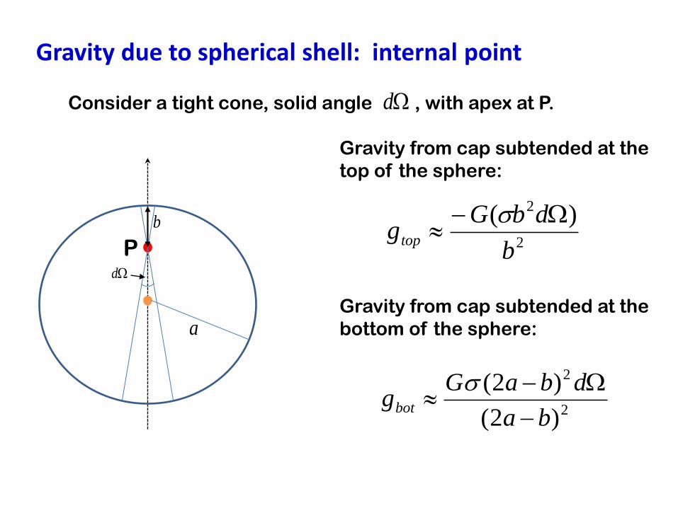
Gravity due to spherical shell: internal point

2

2 )(

b

dbGgtop

P d

a

b

dConsider a tight cone, solid angle , with apex at P.

Gravity from cap subtended at the

top of the sphere:

Gravity from cap subtended at the

bottom of the sphere:

2

2

)2(

)2(

ba

dbaGgbot

Gravity inside a homogeneous sphere

(Blakely, 1995, pp51-53)

z

P

aR

Contribution from material at radii > R

Integrate concentric spherical shells:

where areal density has been replaced

by

a

R

Rr RaGrdrGU 222)(4

dr

Gravity inside a homogeneous sphere (cont’d)

z

P

aR

Contribution from material at radii < R is

Mass of sphere with radius R is ?

Combining contributions from r > R

and r < R:

Therefore gravity varies in ?? fashion with depth

R

GMU Rr

2233

2Ra

GUP

Earth model parameterisation

Geometry, geology, rock properties • “Reduces” non-uniqueness - exclude certain model types • Imposes desired/ achievable resolution. • Defines model volume: 3D spatial extent, relevant data coverage

• Implications for separation of local and regional effects. Prismatic body inversion: cast interpretation in terms of simple geometrical shapes, small number of params => over-determined

“Traditional” quantitative interpretation

For example, use a simple dipping slab model to site an

exploration drill hole. Define 7 parameters: dip,

strike,

density,

depth-to-top,

strike extent,

dip extent, true thickness.

Various formulae: Telford et al., 1990, pp35-46

http://appliedgeophysics.lbl.gov/gravity/index.html

2D Earth model parameterisation: Bosch

Joint inversion of gravity & magnetics

triangular cells, variable in size

stratigraphic => reduce number of property parameters, retain topological significance of contacts

allows heterogeneity within each lithology

finite lateral & vertical extent

parameters are physically different: properties of cells, positions of nodes

geo-statistical characterisation of rock properties for each lithology

Impose geological & petrophysical constraints (as well as geophysical data constraints)

2D parameterisation (Bosch)

(after Bosch & McGaughey, 2001)

property

property

lithology

Physical Property Considerations • Models should honour all geological control (outcrop positions, drillhole

intersections) and petrophysical control (core measurements, borehole logs).

• Physical properties should preferably be measured (on core, or downhole) but

in many cases starting values must be inferred from published tabulations.

• Ideally, define the statistical distribution of physical property for each

geological unit.

• Honour physical property measurements, i.e. assign measured values in their

true 3D locations. In practice, the model cells are usually much larger in volume

than the hand sample (or downhole ‘excitation volume’). Therefore, assignment

of an appropriate value to the model cell enclosing the measurement is not

always straightforward.

• If spatial density of physical property measurements is adequate, the physical

property distribution can be modelled. Options range from simple 3D

interpolation to sophisticated geostatistical modelling. The measured gravity or

other data can serve as constraints on the geostatistical modelling.

Brownfields Exploration Day3 - Lecture 3 22

• The gravitational attraction of a prism at

the origin is:

3D Forward Problem

• Most 3D gravity and magnetic modelling

and inversion codes are based on

discretisation of space into a large number of

prismatic elements:

• There is a linear relationship between Fz and .

Lateral Discretisation

Illustration of a rectangular mesh used to discretise a model (mesh is „floating‟ above the model in this illustration)

3D Earth model parameterisation quantitative property models

UBC-GIF GRAV3D & MAG3D parameterisation: • uniform 3D cell size (over sub-volumes)

• limited (“quantised”) vertical resolution • finite model extents, laterally & vertically • padding cells to reduce edge effects • non-stratigraphic • active parameters are all physically identical: properties of (fixed-size) cells

• numerical inverse problem under-determined

University of British Columbia and some other software developers use a rectangular mesh, regular over sub-volumes if not the entire model volume

3D Earth model parameterisation: VPmg

VPmg parameterisation • uniform cell size in plan • arbitrary size vertically • extends to infinity laterally • extends to arbitrarily large depth • stratigraphic =>

reduce number of property parameters, retain topological significance of contacts

• different styles of inversion: homog. property, heterogeneous property, & geometry • parameters can be different: properties of units & of basement cells, elevations of contacts • numerical inverse problem over- or under-determined or “well-posed”

geological models:

rock type + property

Original rationale for VPmg

• Allow geometry of contacts to adjust in response to the data, but explicitly honour drill hole “pierce points” during inversion

• Generate a model acceptable to both geologists and geophysicists

Distinguishing characteristics of “VP suite”

• Cell boundaries can have geological significance, as contacts, alteration fronts, or structures - no longer arbitrary and artificial

• Cells belong to geological entities

• Therefore, the VP inversion model is a geological model

Geological models

• Geologically constrained inversion comes naturally when inversion

models are … geological

• Geological models are comprised of rock type domains, their

properties, and the boundaries which enclose them

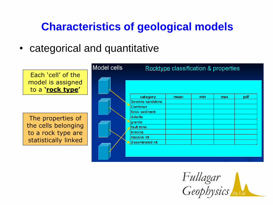
Characteristics of geological models

• categorical and quantitative

Each ‘cell’ of the model is assigned to a ‘rock type’

The properties of the cells belonging to a rock type are statistically linked

VPmg model parameterisation

30

• Vertical rectangular prisms with internal boundaries

• Cells have arbitrary vertical dimension

• Topography incorporated implicitly in model

• Cell boundaries fixed, free, or bounded

• Homogeneous or heterogeneous geological units

• Property bounds assigned to each geological unit

• Heterogeneous basement (extending to great depth)

VP models – Additional Features

Sub-cells for detailed property modelling

Schematic cross-section

31

• Cell thickness arbitrary

• The absence of vertical quantisation permits efficient

representation of thick and thin units and subtle changes in

elevation from prism to prism (left).

• Further sub-division of vertical prisms can occur for detailed

property modelling (right).

Constrained 3D Potential Fields Inversion

Individual vertical prism in a VPmg model

Simple layered model. Green surface represents

topography and the pink-brown surface represents a

geological interface between two units

Close up view of a single

vertical prism; a single elevation

and physical property are stored

for each interface that cuts the

prism

Illustration of all

prisms constituting the

model

1

2

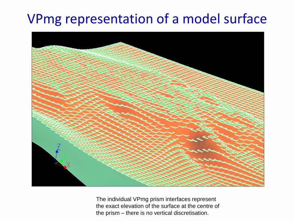
VPmg representation of a model surface

The individual VPmg prism interfaces represent

the exact elevation of the surface at the centre of

the prism – there is no vertical discretisation.

VP model structure supports full 3D complexity

up

Truly 3D body

Cross section through a simple 3D example

…. and permits a variety of model options

Accounting for Regional Effects

• VPmg models are incised into a half space (model does not

abruptly terminate => reduced edge effects)

• VPmg models can be incised into a regional model which is in turn

incised into the half space

• Regional model may be pure basement (apparent density/susc)

• VPmg permits inversion of measured = regional + local (not limited

to local = measured - regional)

Enclo

sing u

nifo

rm h

alf-space

Regional model

Local model

Enclosing uniform half-space

Enclosing uniform half-space

Encl

osi

ng

un

ifo

rm h

alf-

spac

e

Section

Plan

Local model

Regional model

Enclosing uniform half-space

Terrain effects

The accuracy with which the terrain is modelled can be important for gravity interpretation and critical for gravity gradient interpretation.

Terrain correction versus terrain modelling. Terrain models can involve more than one density. VPmg is well suited to terrain modelling & correction: • vertical dimension of cells arbitrary: “unlimited” vertical resolution

• no independent topographic surface: model DTM grid files directly

• no restriction to positive density or susceptibility

• fewer cells in model: faster computation

Regional Terrain

Local Terrain

Regional terrain using same colour scheme as adjacent

image

Local Free Air Gravity Data

Regional terrain for comparison

Regional (surrounding) terrain dominates the survey gravity response

Gravity response of alluvium A layer of alluvium also exists beneath the terrain in the

valley with a density significantly less than other material.

Colour depicts the alluvium thickness (m) in both graphics

3D perspective representation of the terrain. Alluvium thickness is illustrated as a coloured

property on the topography surface

V.A. = 5

Computed gravity response of alluvium + terrain model

Regional terrain for comparison

As expected, the regional terrain dominates the computed gravity response

Terrain-corrected local gravity data

Corrected gravity data reveals anomalies that relate to known geology

Detailed terrain modelling

If < 2*DX

and relief appreciable,

perform detailed terrain correction prior to inversion

topography

= actual measurement station

= topographic wavelength = model cell dimension DX

discretised ground surface

Constrained 3D Potential Fields Inversion

SOG Environs Infrastructure

SOG Pit : ~ 800m x 600m x 270m

Tower Hill Pit: ~ 500m x 150m x 70m

Main waste Dumps: Up to 1000m x 700m x50m

Tailing Dams: up to 1000m x 1000m x 20m

Mt Leonora

WD

TH

WD

WD

WD

TD

TD

SOG

Looking to the North

(Jackson et al., 2004)

Constrained 3D Potential Fields Inversion

Waste/Tails corrected data

0 1 2 3 40.5

Kilometers

-38-37-36-35-33-32-31-30-28-27-26-25-23-22-21-20-18-17-16

Gravitymgal

0 1 2 3 40.5

Kilometers

-37.1-35.9-34.7-33.6-32.5-31.1-30.0-28.9-27.8-26.9-25.6-24.2-22.8-21.6-20.1-19.0-18.2-16.9-15.8

mgal

FREE AIR W/T Corrected FA

VPmg forward algorithm for gravity

Volume integral

Surface integral

Line integral

Gauss’ Theorem

Green’s Theorem

Gravity of a homogeneous rectangular prism The gravity vector outside an arbitrary body of uniform density, , can be written as an integral over the body volume (Coggon, 1976) (1) where G is the universal constant of gravitation, represents the gradient with respect to the observation point, and is the distance between the observation point and a point within the body. The component, , in the z-direction is then given by (2) where is the unit vector in that (arbitrary) direction.

||

0r

dvGg

||

ˆ0

r

dvzGg z

0

|| r

zg

z

The volume integral can be converted to a surface integral by noting that (3) where represents the gradient with respect to the internal (body) point. Substituting from (3) into (2) and invoking Gauss’ Theorem, (4) where denotes the outward unit normal vector to the body surface. The expression in (4) is completely general. However, if represents the vertical direction vector, it follows that the vertical gravity due to any vertically-sided generalised cylinder can be computed as surface integrals over its top and bottom. If, furthermore, the top and bottom are planar, the surface integrals can be reduced to line integrals around the edges.

||

ˆ

||

1ˆ

0r

z

rz

dsr

nzGg z

||

ˆˆ

z

Gravity of a homogeneous rectangular prism: cont’d

n

According to Green’s Theorem in the plane (e.g. Kreyszig, 1967, p313), (5) for a differentiable function f(x,y). Therefore, (4) can be evaluated as a contour integral if a function f can be found with x-derivative (6)

The required function is (7) f x y n x x x x y y z z( , ) ( ) ( ) ( ) 0 0

2

0

2

0

f

xdxdy fdy

CS

f

x r x x y y z z

1 1

0

2

0

2

0

2| | ( ) ( ) ( )

Gravity of a homogeneous rectangular prism: cont’d

If we limit attention to a vertical rectangular prism, with sides oriented parallel to the x- and y-axes, its vertical gravity anomaly reduces to a summation of four definite integrals of the form (8) where (for an observation point at the origin) (9) An analytic expression for F was derived by Fullagar (1975), viz. (10) where the branch of the arctangent function must be chosen to ensure that (11)

),,(),,( 12

2

1

yzxFyzxFdyrxnG

y

y

222 zyxr

z

yrxzrynxyrxnyGyzxF 1tan.2..),,(

sgn tan ... sgn 2 1

2 11

2

z y yy

y

Gravity of a homogeneous rectangular prism: cont’d

VPmg forward algorithm for gravity

Thus, calculation of gravity for homogeneous rectangular prism reduces to eight evaluations of function F at the vertices. For the rectangular cells comprising a “vertical prism” in a VPmg model, only 4 evaluations of function F are required for each additional cell. The function evaluations for a particular horizontal face are “weighted” by the density contrast across the face.

1. Effect of prism size 2. Relationship between prism size and data spacing 3. Effect of data placement: collinear with prism edges; near prism corners 4. Effect of data height

Some modelling considerations

Discretisation effects in forward modelling

= actual measurement station

= gridded upward continued measurement station

Small computational errors can arise, depending on exact placement of data points on stepped model surface. Minimised by gridding to cell centres (and by detailed terrain correction)

VPmg forward algorithm for gravity

Volume integral

Surface integral

Line integral

Gauss’ Theorem

Green’s Theorem

Useful approximation at large distances: approximate as point mass at cell centre

Useful approximation at medium distances: combine contributions from face centres

Exact calculation

3

0

0

3

0

00

||

)(

||

)()(

rr

zzVG

rr

dvzzGrg

c

cz

If a cell is far from the observation point, then where V is the volume of the cell and where is the position vector of the cell centre. If a cell is a moderate distance from the observation point, then where A is the area of the cell top or bottom, and where is the position vector of the cell face.

cr

Volume integral approximation at far offset

0||

ˆˆ

rr

AGds

r

nzGg

s

z

Surface integral approximation at intermediate offset

sr

Introduction to VPmg Files

VPmg File Types

3 or 4 Files required: 1. Control file: define model files and inversion parameters

2. Data file: column ASCII (X,Y,Z,value)

3. Model file: starting model inverted model + calculated responses

4. Par file: define data file and its format specify components for multi-channel cases

1 -3 -58 50000 0 !IGRAV, DEC, INC, AMB, IDH

0 1 2 !IREGNL, ILOCAL, IDL

DUMMY !Local model file

P_rev_6.den !Regional model file

8 0.1 !ITMAX, ERR

0.025 0.02 !PERT, DELD

grav_200.dat !Data file

P_rev_6.008 !Output model file

VPmg control file

PERT = maximum fractional change in contact depths per iteration

DELD = maximum absolute change in unit properties per iteration

constrain size of perturbation

Model parameters: cell size, areal extent, unit properties & bounds, etc.

VPmg model file structure

Geological unit geometry & elevation constraints: east, north, topo_RL, flag, {contact_RL, flag}

Basement topography & properties:

east, north, basement_RL, property

Heterogeneous unit properties & constraints

east, north, ncell, {unit, property, flag}

Observed data & calculated responses: data_east, data_north, data_RL, observed, calculated, background

Start of VPmg model file

Introduction to VPview

(VPmg user interface)

VPview

written by John Paine, Scientific Computing & Applications, Adelaide

Define inversion files & parameters

Create simple layered models Define model parameters

Defining rock properties for geological units

Magnetic model

Density model bounds

remanent properties

VPview display options:

Vertical section

VPview display options:

Horizontal fliche

References Blakely, R.J., 1995, Potential Theory in Gravity & Magnetic Applications: Cambridge University Press, 441p.

Bosch, M., and McGaughey, W.J., 2001, The Leading Edge, 877-881.

Coggon, J.H., 1976, Magnetic and gravity anomalies of polyhedra: Geoexploration, 14, 93-105.

Fullagar, P.K., 1975, Interpretation of underground gravity profiles from the North Broken Hill Mine: B.Sc.(Hons) thesis, Monash University.

Fullagar, P.K., 1998, Program graVP Technical Documentation: Fullagar Geophysics Pty Ltd Memorandum FGR01-01.

Kreyszig, E., 1967, Advanced Engineering Mathematics, 2nd Edition: John Wiley & Sons, 898p.

Telford, W.M., Geldart, L.P., and Sheriff, R.E., 1990, Applied Geophysics: Cambridge University Press, 770p.