Embed Size (px)
Citation preview

Page 1
Errors in Oct 2012 print run (last updated 16 December 2015) NOTE: All of the errors listed here (apart from those
highlighted in yellow) have been fixed in the print run that is due to start selling from early 2016
Page 14, Fig 1.14: There should be a link from "Height" to "Intelligence" in
the lower model. (fixed in Dec 2012 print run) Page 22, Fig 1.21: There should be no link from "Sex" to "Drug taken" in the
middle model of Fig 1.21. (apparently the Dec 2012 print run attempted to fix this but changed the wrong part of the figure). The correct figures are:
Page 32, Fig 2.1 should be the same as Fig 1.13. Specifically, the formula
should say "N=2.144 x T + 243.55" not "N=2.144 > T + 243.55" (thanks to Chris Hobbs for noticing that)
Page 44, Figure 2.13b: Replace the bubble text “Loss of life” with “Loss of
Capital”. (thanks to Fredrik Bökman for noticing that)
Page 45: Second bullet at the bottom of the page, should be “So a ‘Law suit’
or ‘Flood’ is obviously a worse outcome” rather than the current reading of “better outcome”.
(thanks to Richard Austin for noticing that)
Page 53: Box 3.1 Point 7. Replace “..experiment of O.J. Simpson being tried for murder” with “..experiment of observing the death of O.J.Simpson’s ex-wife” Page 53: Box 3.1 Point 8. Replace “..testing you for cancer” with “..testing you for cancer (assuming a perfectly accurate test)”
(thanks to Fredrik Bökman for noticing that) Page 71, box 4.1 last 2 lines: Replace:
“..the bookmaker will only have to pay out on average $80 for each $100 gambled, yielding a profit margin of 20%."
with
Page 2
“..the bookmaker will only have to pay out on average $90 for each $100 gambled, yielding a profit margin of 10% (profit margin is defined as: profit as percentage of selling price or revenue, i.e. 10/100) "
(thanks to PD and Andrew Rattray for noticing that)
Page 75: line -4 "..is shorthand for the sum of the terms..." should be
replaced by "...is shorthand for the product of the terms...." (thanks to Teresa Zigh for noticing that)
Page 78, Theorem 4.2: Should be:
𝑃(𝐴 ∪ 𝐵) = 𝑃(𝐴) + 𝑃(𝐵) − 𝑃(𝐴 ∩ 𝐵)
(fixed in Dec 2012 print run) (thanks to Mark Blackburn for noticing that)
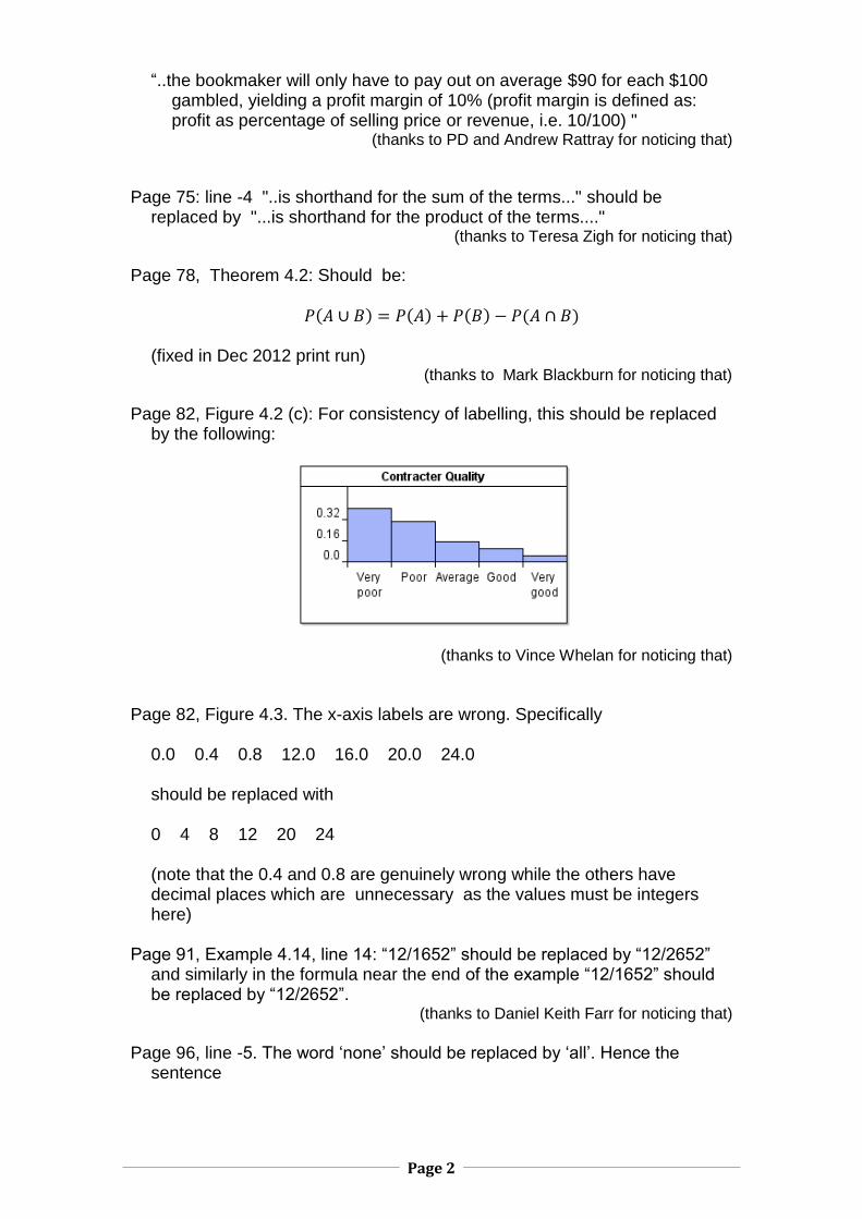
Page 82, Figure 4.2 (c): For consistency of labelling, this should be replaced
by the following:
(thanks to Vince Whelan for noticing that)
Page 82, Figure 4.3. The x-axis labels are wrong. Specifically
0.0 0.4 0.8 12.0 16.0 20.0 24.0 should be replaced with 0 4 8 12 20 24 (note that the 0.4 and 0.8 are genuinely wrong while the others have decimal places which are unnecessary as the values must be integers here)
Page 91, Example 4.14, line 14: “12/1652” should be replaced by “12/2652”
and similarly in the formula near the end of the example “12/1652” should be replaced by “12/2652”.
(thanks to Daniel Keith Farr for noticing that)
Page 96, line -5. The word ‘none’ should be replaced by ‘all’. Hence the
sentence
Page 3
“It is just as easy to calculate P(5), the probability that none of the five components fails..”
Should say “It is just as easy to calculate P(5), the probability that all of the five
components fails..” (thanks to Hashmat Mastin for noticing that)
Page 100. The last two lines above Box 4.11. Replace
"..so in this case the mean number of bugs remaining is 1.8" with "..so in this case the mean number of bugs found is 18, and the mean
number of bugs remaining is 2". (thanks to Teresa Zigh for noticing that)
Page 101, Box 4.12, line 2. There are two errors here: “without replacement”
should be “with replacement”; and 35623 should be 36523. (thanks to Yun Wang for noticing that)
The same error (where the number 365 was wrongly written as 356) actually occurs in three other places in the box. Here is the correct version of the 4
th
and 5th sentences (with the change shown in bold):
So any specific assignment of birthdays has a probability of 1/365
23. That
means, for example, that the probability that every child was born on January 1 is 1/365
23 and the probability that 10 were born on May 18 and
13 were born on September 30 is also 1/36523
.
Page 101, line under first formula: Replace ”where sampling is not allowed”,
with ”replacement”. (thanks to Fredrik Bökman for noticing that)
Page 101, Box 4.12.
Page 105, line 7, replace
"But it is usually the case that the probability of such events is much lower than stated.” with "But it is usually the case that the probability of such events is much higher than stated.”
(thanks to Ian McDavid for noticing that) Page 106 (Example 4.23) has a number of errors, the most serious arising
from the simple arithmetic error in the final equation where the answer given is 0.9423 instead of 1-0.9423 = 0.0577 (thanks to Mark Woolley for alerting us to the problems in this example). The full set of changes needed are:
Line 1. Replace:
Page 4
“In fact, even this apparently amazing event is not at all unlikely. Over a 20-year period it is almost certain that at least one of the 300 national lotteries will have two consecutive draws with the same numbers.”
with “In fact, even this apparently amazing event is not so unusual when we
consider, say, a 20-year period and the fact that there are about 300 different national lotteries (some countries have several).”
Line 6: Replace
“Chapter 3, Example 3.7” with “Chapter 3, Example 3.6”
Line 7:
Replace “1/5247785” with “1/5245786”
Line 14: In the formula, replace “5245785” with “5245786” Line 22 (last line of formula). Replace
“=0.9423” with “=1 – 0.9423 = 0.0577”
Line 23 (last line of Example 4.23). Replace:
“So, the probability of this happening is very high” with “So, the probability of this happening is just under 6%”
Page 122-123. Example 5.6. There are several errors in here and in the
sidebar. In the sidebar, replace “It turns out that the 99th percentile in this case is 62. This means the
probability of at least 62 heads in 100 tosses of a fair coin is 0.01” with “It turns out that the 99th percentile in this case is between 62 and 63. The
probability of at least 62 heads in 100 tosses of a fair coin is approximately 0.0105 and the probability of at least 63 heads is 0.006”
Replace the main text of Example 5.6 (starting at the beginning “Suppose
we have…” on page 122 up to and including the formula on page 123) with the following
Suppose that we have 999 fair coins and one coin that is known to be biased toward ‘heads’. We assume that the probability of tossing a ‘head’ is 0.5 for a fair coin and 0.9 for a biased coin. We select a coin randomly. We now wish to test the null hypothesis that the coin is not biased. To do this we toss the coin 100 times and record the number of heads, X. As good experimenters we set a significance level in advance at a value of 0.01. What this means is that if we observe a p-value less
Page 5
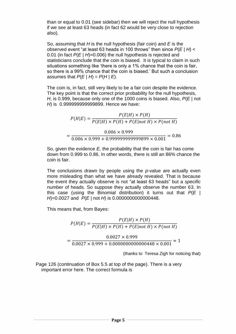
than or equal to 0.01 (see sidebar) then we will reject the null hypothesis if we see at least 63 heads (in fact 62 would be very close to rejection also). So, assuming that H is the null hypothesis (fair coin) and E is the observed event “at least 63 heads in 100 throws” then since P(E | H) < 0.01 (in fact P(E | H)=0.006) the null hypothesis is rejected and statisticians conclude that the coin is biased. It is typical to claim in such situations something like ‘there is only a 1% chance that the coin is fair, so there is a 99% chance that the coin is biased.’ But such a conclusion assumes that P(E | H) = P(H | E). The coin is, in fact, still very likely to be a fair coin despite the evidence. The key point is that the correct prior probability for the null hypothesis, H, is 0.999, because only one of the 1000 coins is biased. Also, P(E | not H) is 0.999999999999899. Hence we have:
𝑃(𝐻|𝐸) =𝑃(𝐸|𝐻) × 𝑃(𝐻)
𝑃(𝐸|𝐻) × 𝑃(𝐻) + 𝑃(𝐸|𝑛𝑜𝑡 𝐻) × 𝑃(𝑛𝑜𝑡 𝐻)
=0.006 × 0.999
0.006 × 0.999 + 0.999999999999899 × 0.001= 0.86
So, given the evidence E, the probability that the coin is fair has come down from 0.999 to 0.86. In other words, there is still an 86% chance the coin is fair. The conclusions drawn by people using the p-value are actually even more misleading than what we have already revealed. That is because the event they actually observe is not “at least 63 heads” but a specific number of heads. So suppose they actually observe the number 63. In this case (using the Binomial distribution) it turns out that P(E | H)=0.0027 and P(E | not H) is 0.0000000000000448. This means that, from Bayes:
𝑃(𝐻|𝐸) =𝑃(𝐸|𝐻) × 𝑃(𝐻)
𝑃(𝐸|𝐻) × 𝑃(𝐻) + 𝑃(𝐸|𝑛𝑜𝑡 𝐻) × 𝑃(𝑛𝑜𝑡 𝐻)
=0.0027 × 0.999
0.0027 × 0.999 + 0.0000000000000448 × 0.001≈ 1
(thanks to Teresa Zigh for noticing that)
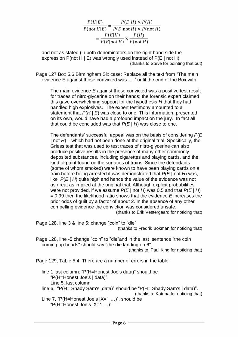
Page 126 (continuation of Box 5.5 at top of the page). There is a very
important error here. The correct formula is
Page 6
𝑃(𝐻|𝐸)
𝑃(not 𝐻|𝐸)=
𝑃(𝐸|𝐻) × 𝑃(𝐻)
𝑃(𝐸|not 𝐻) × 𝑃(not 𝐻)
=𝑃(𝐸|𝐻)
𝑃(𝐸|not 𝐻)×
𝑃(𝐻)
𝑃(not 𝐻)
and not as stated (in both denominators on the right hand side the expression P(not H | E) was wrongly used instead of P(E | not H).
(thanks to Steve for pointing that out)
Page 127 Box 5.6 Birmingham Six case: Replace all the text from “The main
evidence E against those convicted was ….” until the end of the Box with:
The main evidence E against those convicted was a positive test result for traces of nitro-glycerine on their hands; the forensic expert claimed this gave overwhelming support for the hypothesis H that they had handled high explosives. The expert testimony amounted to a statement that P(H | E) was close to one. This information, presented on its own, would have had a profound impact on the jury. In fact all that could be concluded was that P(E | H) was close to one.
The defendants’ successful appeal was on the basis of considering P(E | not H) – which had not been done at the original trial. Specifically, the Griess test that was used to test traces of nitro-glycerine can also produce positive results in the presence of many other commonly deposited substances, including cigarettes and playing cards, and the kind of paint found on the surfaces of trains. Since the defendants (some of whom smoked) were known to have been playing cards on a train before being arrested it was demonstrated that P(E | not H) was, like P(E | H) quite high and hence the value of the evidence was not as great as implied at the original trial. Although explicit probabilities were not provided, if we assume P(E | not H) was 0.5 and that P(E | H) = 0.99 then the likelihood ratio shows that the evidence E increases the prior odds of guilt by a factor of about 2. In the absence of any other compelling evidence the conviction was considered unsafe.
(thanks to Erik Vestergaard for noticing that)
Page 128, line 3 & line 5: change ”coin” to ”die”
(thanks to Fredrik Bökman for noticing that) Page 128, line -5 change ”coin” to ”die”and in the last sentence "the coin
coming up heads" should say "the die landing on 6". (thanks to Paul King for noticing that)
Page 129, Table 5.4: There are a number of errors in the table:
line 1 last column: “P(H=Honest Joe's data)” should be “P(H=Honest Joe's | data)”. Line 5, last column
line 6, “P(H= Shady Sam's data)” should be “P(H= Shady Sam's | data)”. (thanks to Katrina for noticing that)
Line 7, “P(H=Honest Joe’s |X=1 …)”, should be “P(H=Honest Joe’s |X=1 …)”
Page 7
(thanks to Fredrik Bökman for noticing that)
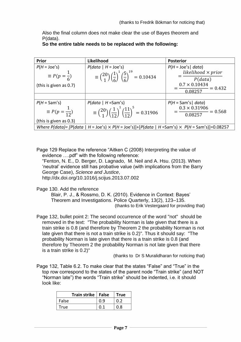
Also the final column does not make clear the use of Bayes theorem and P(data). So the entire table needs to be replaced with the following:
Prior Likelihood Posterior
P(H = Joe’s) P(data | H = Joe’s) P(H = Joe’s| data)
≡ 𝑃(𝑝 =1
6) ≡ (
201
) (1
6)
1
(5
6)
19
= 0.10434 =𝑙𝑖𝑘𝑒𝑙𝑖ℎ𝑜𝑜𝑑 × 𝑝𝑟𝑖𝑜𝑟
𝑃(𝑑𝑎𝑡𝑎)
(this is given as 0.7) =
0.7 × 0.10434
0.08257= 0.432
P(H = Sam’s) P(data | H =Sam’s) P(H = Sam’s| data)
≡ 𝑃(𝑝 =1
12) ≡ (
201
) (1
12)
1
(11
12)
5
= 0.31906 =0.3 × 0.31906
0.08257= 0.568
(this is given as 0.3)
Where P(data)= [P(data | H = Joe’s) × P(H = Joe’s)]+[P(data | H =Sam’s) × P(H = Sam’s)]=0.08257
Page 129 Replace the reference “Aitken C (2008) Interpreting the value of evidence ….pdf” with the following reference: “Fenton, N. E., D. Berger, D. Lagnado, M. Neil and A. Hsu. (2013). When ‘neutral’ evidence still has probative value (with implications from the Barry George Case), Science and Justice, http://dx.doi.org/10.1016/j.scijus.2013.07.002
Page 130. Add the reference
Blair, P. J., & Rossmo, D. K. (2010). Evidence in Context: Bayes’ Theorem and Investigations. Police Quarterly, 13(2), 123–135.
(thanks to Erik Vestergaard for providing that)
Page 132, bullet point 2: The second occurrence of the word "not" should be
removed in the text: "The probability Norman is late given that there is a train strike is 0.8 (and therefore by Theorem 2 the probability Norman is not late given that there is not a train strike is 0.2)". Thus it should say: "The probability Norman is late given that there is a train strike is 0.8 (and therefore by Theorem 2 the probability Norman is not late given that there is a train strike is 0.2)"
(thanks to Dr S Muralidharan for noticing that)
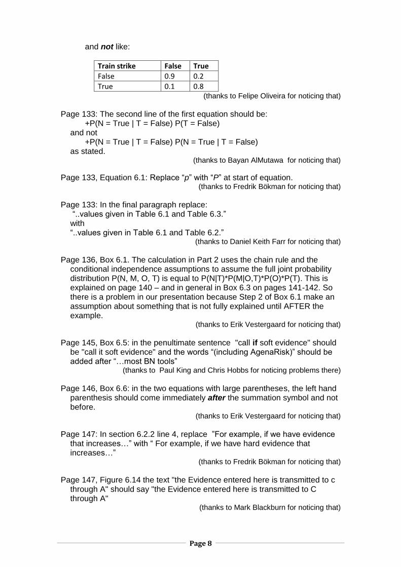
Page 132, Table 6.2. To make clear that the states “False” and “True” in the top row correspond to the states of the parent node “Train strike” (and NOT “Norman late”) the words “Train strike” should be indented, i.e. it should look like:
Train strike False True
False 0.9 0.2
True 0.1 0.8
Page 8
and not like:
Train strike False True
False 0.9 0.2
True 0.1 0.8 (thanks to Felipe Oliveira for noticing that)
Page 133: The second line of the first equation should be:
+P(N = True | T = False) P(T = False) and not
+P(N = True | T = False) P(N = True | T = False) as stated.
(thanks to Bayan AlMutawa for noticing that)
Page 133, Equation 6.1: Replace “p” with “P” at start of equation. (thanks to Fredrik Bökman for noticing that)
Page 133: In the final paragraph replace:
“..values given in Table 6.1 and Table 6.3.” with “..values given in Table 6.1 and Table 6.2.”
(thanks to Daniel Keith Farr for noticing that)
Page 136, Box 6.1. The calculation in Part 2 uses the chain rule and the
conditional independence assumptions to assume the full joint probability distribution P(N, M, O, T) is equal to P(N|T)*P(M|O,T)*P(O)*P(T). This is explained on page 140 – and in general in Box 6.3 on pages 141-142. So there is a problem in our presentation because Step 2 of Box 6.1 make an assumption about something that is not fully explained until AFTER the example.
(thanks to Erik Vestergaard for noticing that)
Page 145, Box 6.5: in the penultimate sentence "call if soft evidence" should
be "call it soft evidence" and the words “(including AgenaRisk)” should be added after “…most BN tools”
(thanks to Paul King and Chris Hobbs for noticing problems there)
Page 146, Box 6.6: in the two equations with large parentheses, the left hand
parenthesis should come immediately after the summation symbol and not before.
(thanks to Erik Vestergaard for noticing that)
Page 147: In section 6.2.2 line 4, replace ”For example, if we have evidence
that increases…” with “ For example, if we have hard evidence that increases…”
(thanks to Fredrik Bökman for noticing that)
Page 147, Figure 6.14 the text "the Evidence entered here is transmitted to c
through A" should say "the Evidence entered here is transmitted to C through A"
(thanks to Mark Blackburn for noticing that)
Page 9
Page 148, Box 6.7: Second line of the formula should have the brackets
inside, i.e. should be:
= ∑ (𝑃(𝐶|𝐴 = 𝑎) (∑ 𝑃(𝐵|𝐴 = 𝑎)
𝐵
) 𝑃(𝐴 = 𝑎))
𝐴
(thanks to Fredrik Bökman for noticing that)
Page 149, Box 6.7: Second line of the formula should have the brackets inside (i.e. similar change as above)
(thanks to Fredrik Bökman for noticing that)
Page 153, Box 6.10 “Mathematical Notation for Independence”. The text
inside this box should be replaced with the following:
For compactness, some other books use a special mathematical symbol ⊥ to specify whether variables are conditionally or marginally independent of one another. Specifically:
1. (X ⊥Y) | Z=z means that X is independent of Y given hard evidence z for Z. For example, in Figure 6.9 and in Figure 6.12 we have (B⊥C)|A=a because in the former we have a serial d-connection through A and in the latter we have a diverging d-connection from A.
2. (X⊥Y) | Z means that X is independent of Y given no evidence in Z. For example, in Figure 6.16 (where there is converging connection on A) we
would write (B⊥C) | A (thanks toJaime Villalpando for noticing that)
Page. 158, Table 6.6: In columns 3, 11, 19 (corresponding to “Red, Red,
Stick”, “Green, Green, Stick”, “Blue, Blue, Stick”) all the numbers should all be set to 0.33 (as in the columns to their left). Although it makes no difference to the result this is to be consistent with the comment in the sidebar on page 159
(thanks to Robbie Hearmans for noticing that) Page 161 In bullet describing Model b, replace “This has three two nodes …”
with “This has three nodes …” (thanks to Andrew Steckley for noticing that)
Page 162, line 7: ”Figures 6.30 and 6.35” should be ”Figures 6.30 and 6.31”
(thanks to Fredrik Bökman for noticing that)
Page 167, line 3 in Box 6.11: “Section 6.5.1” should be “Section 6.6.1”
(thanks to Fredrik Bökman for noticing that)
Page 168, line 2: “Box 6.6” should be “Box 6.5”
(thanks to Fredrik Bökman for noticing that)
Page 189: Figure 7.31b: Apparently in some print-runs the word ”project” has
turned into a box, a non-character. (thanks to Fredrik Bökman for noticing that)
Page 10
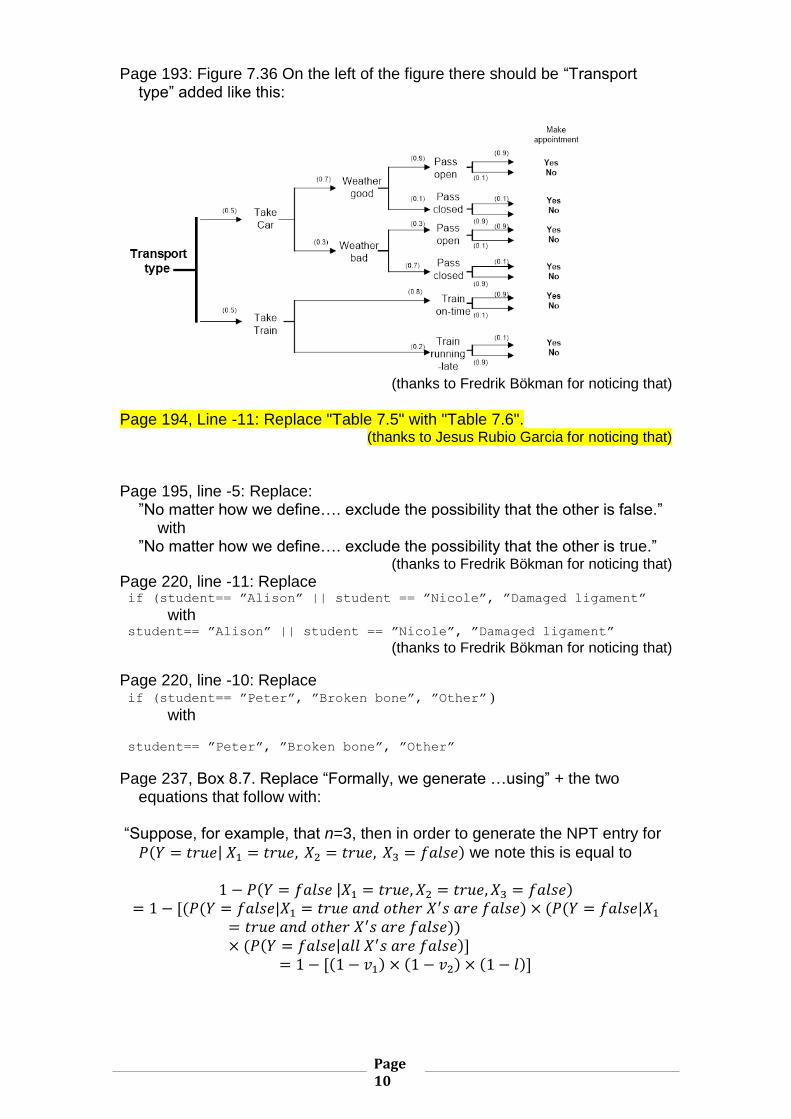
Page 193: Figure 7.36 On the left of the figure there should be “Transport type” added like this:
(thanks to Fredrik Bökman for noticing that)
Page 194, Line -11: Replace "Table 7.5" with "Table 7.6".
(thanks to Jesus Rubio Garcia for noticing that)
Page 195, line -5: Replace:
”No matter how we define…. exclude the possibility that the other is false.” with
”No matter how we define…. exclude the possibility that the other is true.” (thanks to Fredrik Bökman for noticing that)
Page 220, line -11: Replace if (student== ”Alison” || student == ”Nicole”, ”Damaged ligament”
with student== ”Alison” || student == ”Nicole”, ”Damaged ligament”
(thanks to Fredrik Bökman for noticing that)
Page 220, line -10: Replace if (student== ”Peter”, ”Broken bone”, ”Other” )
with
student== ”Peter”, ”Broken bone”, ”Other”
Page 237, Box 8.7. Replace “Formally, we generate …using” + the two equations that follow with:
“Suppose, for example, that n=3, then in order to generate the NPT entry for
𝑃(𝑌 = 𝑡𝑟𝑢𝑒| 𝑋1 = 𝑡𝑟𝑢𝑒, 𝑋2 = 𝑡𝑟𝑢𝑒, 𝑋3 = 𝑓𝑎𝑙𝑠𝑒) we note this is equal to
1 − 𝑃(𝑌 = 𝑓𝑎𝑙𝑠𝑒 |𝑋1 = 𝑡𝑟𝑢𝑒, 𝑋2 = 𝑡𝑟𝑢𝑒, 𝑋3 = 𝑓𝑎𝑙𝑠𝑒) = 1 − [(𝑃(𝑌 = 𝑓𝑎𝑙𝑠𝑒|𝑋1 = 𝑡𝑟𝑢𝑒 𝑎𝑛𝑑 𝑜𝑡ℎ𝑒𝑟 𝑋′𝑠 𝑎𝑟𝑒 𝑓𝑎𝑙𝑠𝑒) × (𝑃(𝑌 = 𝑓𝑎𝑙𝑠𝑒|𝑋1
= 𝑡𝑟𝑢𝑒 𝑎𝑛𝑑 𝑜𝑡ℎ𝑒𝑟 𝑋′𝑠 𝑎𝑟𝑒 𝑓𝑎𝑙𝑠𝑒))× (𝑃(𝑌 = 𝑓𝑎𝑙𝑠𝑒|𝑎𝑙𝑙 𝑋′𝑠 𝑎𝑟𝑒 𝑓𝑎𝑙𝑠𝑒)]
= 1 − [(1 − 𝑣1) × (1 − 𝑣2) × (1 − 𝑙)]
Page 11
Page 240, line -4: Remove the text "which is 90%" at the end of the sentence.
(thanks to Jesus Rubio Garcia for noticing that)
Page 247, last line of Tabel 8.10: Repalce “State n-1” with “State n”. Page 248, Figure 8.31 The two examples in the first column, rows 2 and 3
should be TNormal(0.5, 0.1) and TNormal (0.5, 0.01) (thanks to Mark Blackburn for noticing that)
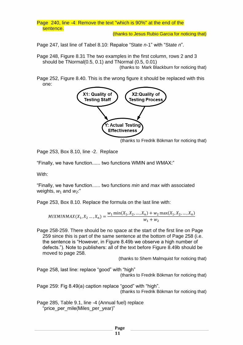
Page 252, Figure 8.40. This is the wrong figure it should be replaced with this
one:
(thanks to Fredrik Bökman for noticing that)
Page 253, Box 8.10, line -2. Replace “Finally, we have function...... two functions WMIN and WMAX:” With:
“Finally, we have function...... two functions min and max with associated weights, w1 and w2:”
Page 253, Box 8.10. Replace the formula on the last line with:
𝑀𝐼𝑋𝑀𝐼𝑁𝑀𝐴𝑋(𝑋1, 𝑋2 … , 𝑋𝑛) =𝑤1 min(𝑋1, 𝑋2, … , 𝑋𝑛) + 𝑤2 max(𝑋1, 𝑋2, … , 𝑋𝑛)
𝑤1 + 𝑤2
Page 258-259. There should be no space at the start of the first line on Page
259 since this is part of the same sentence at the bottom of Page 258 (i.e. the sentence is “However, in Figure 8.49b we observe a high number of defects.”). Note to publishers: all of the text before Figure 8.49b should be moved to page 258.
(thanks to Shem Malmquist for noticing that)
Page 258, last line: replace “good” with “high”
(thanks to Fredrik Bökman for noticing that)
Page 259: Fig 8.49(a) caption replace “good” with “high”.
(thanks to Fredrik Bökman for noticing that)
Page 285, Table 9.1, line -4 (Annual fuel) replace
“price_per_mile(Miles_per_year)”
Page 12
with price_per_mile × Miles_per_year
(thanks to Fredrik Bökman for noticing that)
Page 287, Line -4 "..standard deviation of 0.25" should say "..standard
deviation of 0.5" Also, in formula on last line "0.25" should say "0.5". (thanks to Thomas Barnett for noticing that)
Page 289-299 (Section 9.5.3): There are a number of issues in this section
that we are currently reviewing and which will result in a significant rewrite. (thanks to Ernest Lever for noticing that)
Page 290, Result of variance formula at the bottom of page should be 0.0347
rather than 0.0344 as stated.
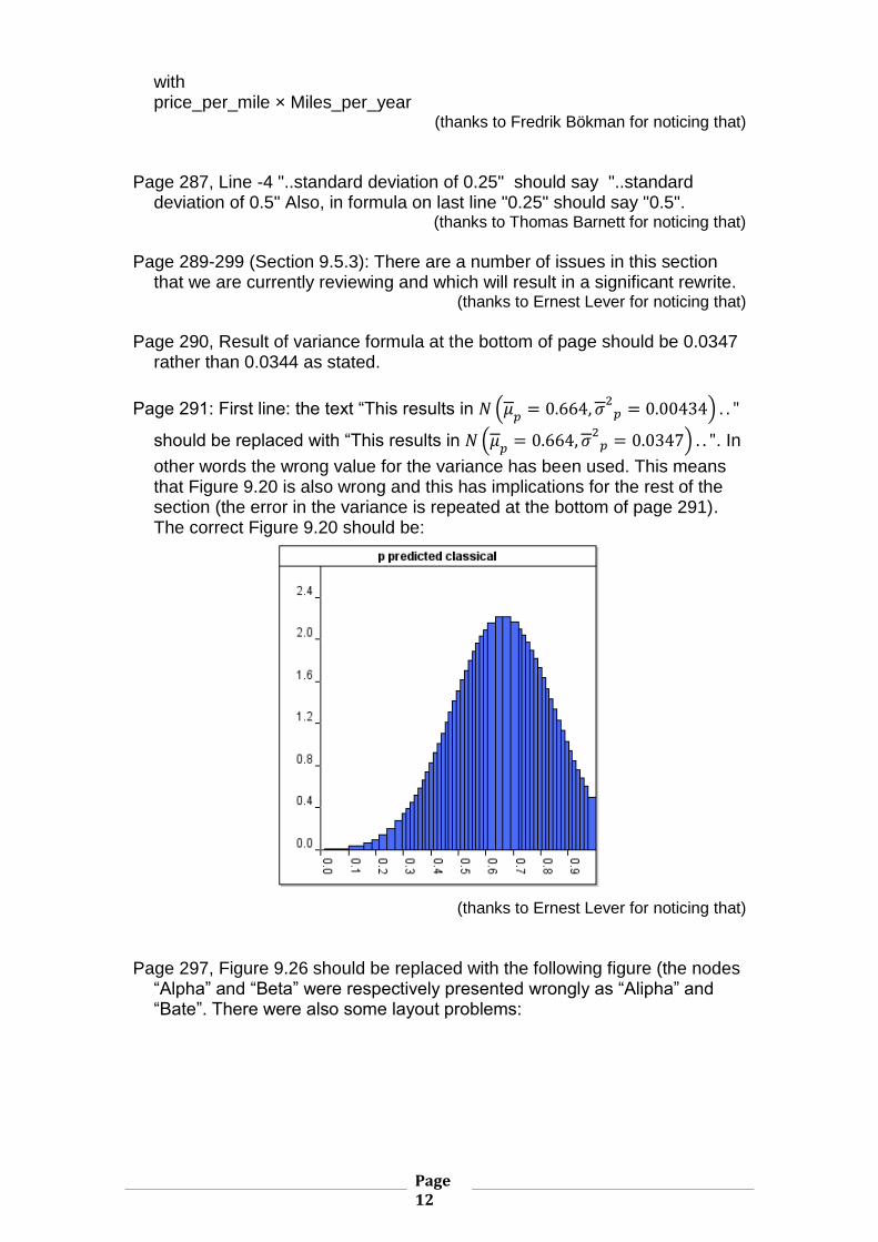
Page 291: First line: the text “This results in 𝑁 (𝜇𝑝
= 0.664, 𝜎2
𝑝 = 0.00434) . . "
should be replaced with “This results in 𝑁 (𝜇𝑝
= 0.664, 𝜎2
𝑝 = 0.0347) . . ". In
other words the wrong value for the variance has been used. This means that Figure 9.20 is also wrong and this has implications for the rest of the section (the error in the variance is repeated at the bottom of page 291). The correct Figure 9.20 should be:
(thanks to Ernest Lever for noticing that)
Page 297, Figure 9.26 should be replaced with the following figure (the nodes
“Alpha” and “Beta” were respectively presented wrongly as “Alipha” and “Bate”. There were also some layout problems:
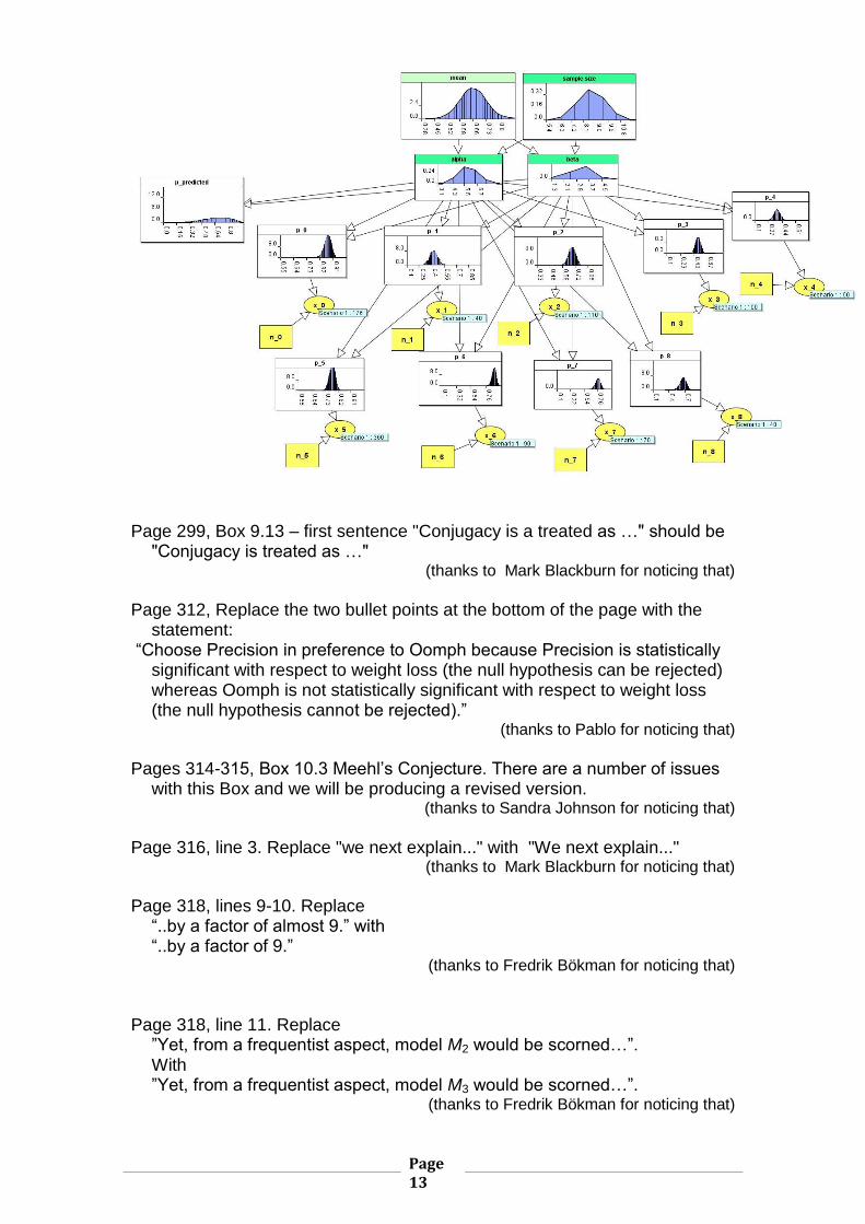
Page 13
Page 299, Box 9.13 – first sentence "Conjugacy is a treated as …" should be
"Conjugacy is treated as …" (thanks to Mark Blackburn for noticing that)
Page 312, Replace the two bullet points at the bottom of the page with the
statement: “Choose Precision in preference to Oomph because Precision is statistically
significant with respect to weight loss (the null hypothesis can be rejected) whereas Oomph is not statistically significant with respect to weight loss (the null hypothesis cannot be rejected).”
(thanks to Pablo for noticing that)
Pages 314-315, Box 10.3 Meehl’s Conjecture. There are a number of issues
with this Box and we will be producing a revised version. (thanks to Sandra Johnson for noticing that)
Page 316, line 3. Replace "we next explain..." with "We next explain..."
(thanks to Mark Blackburn for noticing that)
Page 318, lines 9-10. Replace
“..by a factor of almost 9.” with “..by a factor of 9.”
(thanks to Fredrik Bökman for noticing that)
Page 318, line 11. Replace ”Yet, from a frequentist aspect, model M2 would be scorned…”. With ”Yet, from a frequentist aspect, model M3 would be scorned…”.
(thanks to Fredrik Bökman for noticing that)
Page 14
Page 321, line -8. Replace “(written 𝑑𝐿
𝑑𝑃)” with “(written
𝑑𝐿
𝑑𝑝)” (i.e. small p not P)
(thanks to Fredrik Bökman for noticing that)
Page 321, line -9. First line of the formula should be replaced with
𝑑𝐿
𝑑𝑝=
𝑑
𝑑𝑝𝐾𝑝𝑥(1 − 𝑝)𝑛−𝑥 = ⋯
(there are 2 errors a P which should be p and a missing 𝑑/𝑑𝑝) (thanks to Fredrik Bökman for noticing that)
Page 329 (instruction to publishers): Figure 10.8 is supposed to span the
page. Page 329, immediately before Box 10.9. Replace the sentence “However, you
can get these results by simply running the AgenaRisk model.” With ““All of the detailed results can be obtained simply by running the relevant components of the AgenaRisk model.”
Page 330, Step 2 line 3: Replace “S dependent of V and D” with “S
independent of V and D” (thanks to Jun Wang for noticing that)
Page 331, line 3. Replace “4.26E-06” with ““4.26E-06”
(this is to make it consistent with the scientific notation used elsewhere in the box)
Page 331, line 7. Replace “S dependent on V” with “S dependent on D”
(thanks to Jun Wang for noticing that)
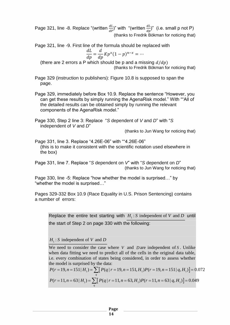
Page 330, line -5: Replace “how whether the model is surprised…” by “whether the model is surprised…” Pages 329-332 Box 10.9 (Race Equality in U.S. Prison Sentencing) contains a number of errors:
Replace the entire text starting with 1 : independent of and H S V D until
the start of Step 2 on page 330 with the following:
1 : independent of and H S V D
We need to consider the case where V and D are independent of S . Unlike
when data fitting we need to predict all of the cells in the original data table,
i.e. every combination of states being considered, in order to assess whether
the model is surprised by the data:
1 1 1( 19, 151| ) ( | 19, 151, ) ( 19, 151| , ) 0.072q
P r n H P q r n H P r n q H
1 1 1( 11, 63 | ) ( | 11, 63, ) ( 11, 63 | , ) 0.049q
P r n H P q r n H P r n q H
Page 15
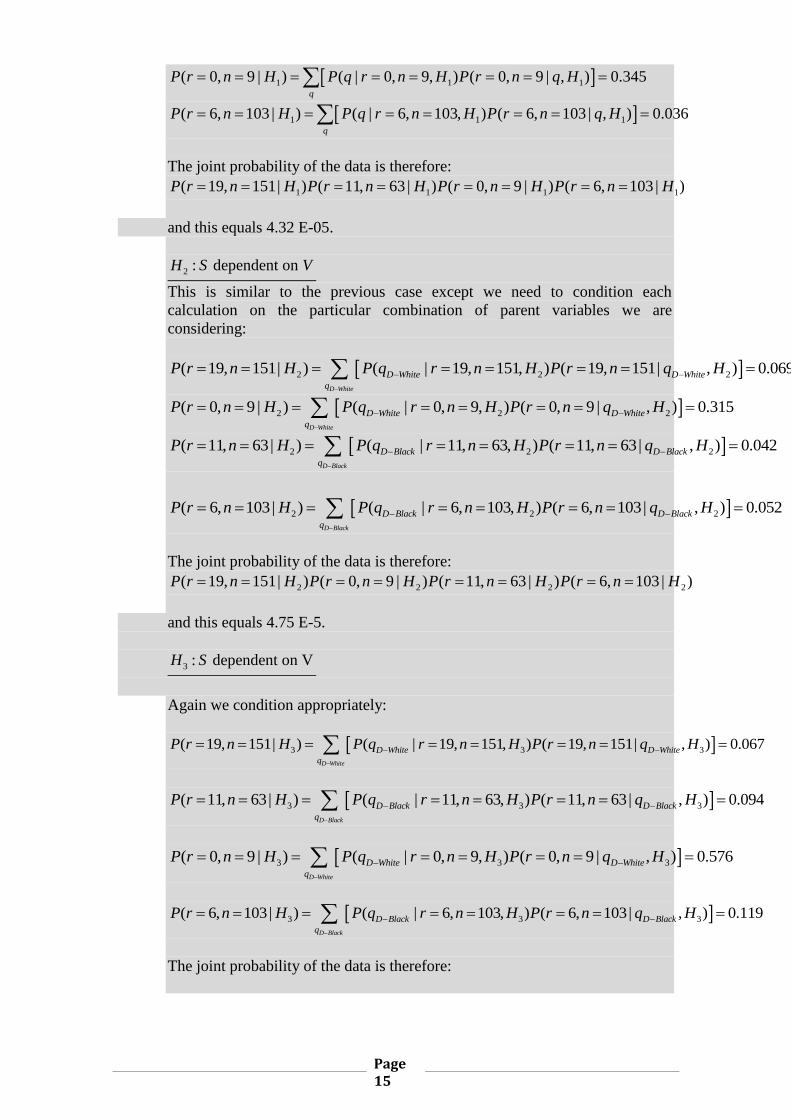
1 1 1( 0, 9 | ) ( | 0, 9, ) ( 0, 9 | , ) 0.345q
P r n H P q r n H P r n q H
1 1 1( 6, 103 | ) ( | 6, 103, ) ( 6, 103 | , ) 0.036q
P r n H P q r n H P r n q H
The joint probability of the data is therefore:
1 1 1 1( 19, 151| ) ( 11, 63 | ) ( 0, 9 | ) ( 6, 103 | )P r n H P r n H P r n H P r n H
and this equals 4.32 E-05.
2 : dependent on H S V
This is similar to the previous case except we need to condition each
calculation on the particular combination of parent variables we are
considering:
2 2 2( 19, 151| ) ( | 19, 151, ) ( 19, 151| , ) 0.069D White
D White D White
q
P r n H P q r n H P r n q H
2 2 2( 0, 9 | ) ( | 0, 9, ) ( 0, 9 | , ) 0.315D White
D White D White
q
P r n H P q r n H P r n q H
2 2 2( 11, 63 | ) ( | 11, 63, ) ( 11, 63 | , ) 0.042D Black
D Black D Black
q
P r n H P q r n H P r n q H
2 2 2( 6, 103| ) ( | 6, 103, ) ( 6, 103| , ) 0.052D Black
D Black D Black
q
P r n H P q r n H P r n q H
The joint probability of the data is therefore:
2 2 2 2( 19, 151| ) ( 0, 9 | ) ( 11, 63 | ) ( 6, 103 | )P r n H P r n H P r n H P r n H
and this equals 4.75 E-5.
3 : dependent on VH S
Again we condition appropriately:
3 3 3( 19, 151| ) ( | 19, 151, ) ( 19, 151| , ) 0.067D White
D White D White
q
P r n H P q r n H P r n q H
3 3 3( 11, 63 | ) ( | 11, 63, ) ( 11, 63 | , ) 0.094D Black
D Black D Black
q
P r n H P q r n H P r n q H
3 3 3( 0, 9 | ) ( | 0, 9, ) ( 0, 9 | , ) 0.576D White
D White D White
q
P r n H P q r n H P r n q H
3 3 3( 6, 103| ) ( | 6, 103, ) ( 6, 103| , ) 0.119D Black
D Black D Black
q
P r n H P q r n H P r n q H
The joint probability of the data is therefore:
Page 16
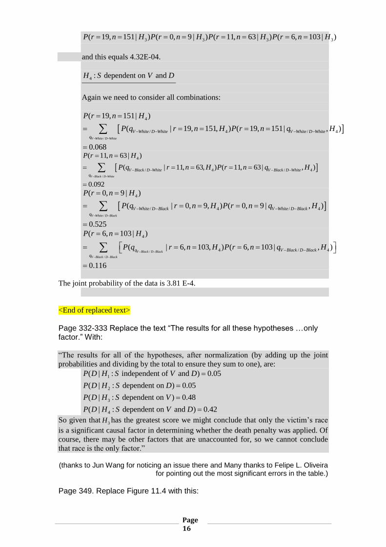
3 3 3 3( 19, 151| ) ( 0, 9 | ) ( 11, 63 | ) ( 6, 103 | )P r n H P r n H P r n H P r n H
and this equals 4.32E-04.
4 : dependent on and H S V D
Again we need to consider all combinations:
/
4
/ 4 / 4
( 19, 151| )
( | 19, 151, ) ( 19, 151| , )
0.068
V White D White
V White D White V White D White
q
P r n H
P q r n H P r n q H
/
4
/ 4 / 4
( 11, 63 | )
( | 11, 63, ) ( 11, 63 | , )
0.092
V Black D White
V Black D White V Black D White
q
P r n H
P q r n H P r n q H
/
4
/ 4 / 4
( 0, 9 | )
( | 0, 9, ) ( 0, 9 | , )
0.525
V White D Black
V White D Black V White D Black
q
P r n H
P q r n H P r n q H
/
/
4
4 / 4
( 6, 103 | )
( | 6, 103, ) ( 6, 103 | , )
0.116
V Black D Black
V Black D Black
q V Black D Black
q
P r n H
P q r n H P r n q H
The joint probability of the data is 3.81 E-4.
<End of replaced text>
Page 332-333 Replace the text “The results for all these hypotheses …only factor.” With:
“The results for all of the hypotheses, after normalization (by adding up the joint
probabilities and dividing by the total to ensure they sum to one), are:
1
2
3
4
( | : independent of and ) 0.05
( | : dependent on ) 0.05
( | : dependent on ) 0.48
( | : dependent on and ) 0.42
P D H S V D
P D H S D
P D H S V
P D H S V D
So given that3H has the greatest score we might conclude that only the victim’s race
is a significant causal factor in determining whether the death penalty was applied. Of
course, there may be other factors that are unaccounted for, so we cannot conclude
that race is the only factor.”
(thanks to Jun Wang for noticing an issue there and Many thanks to Felipe L. Oliveira for pointing out the most significant errors in the table.)
Page 349. Replace Figure 11.4 with this:
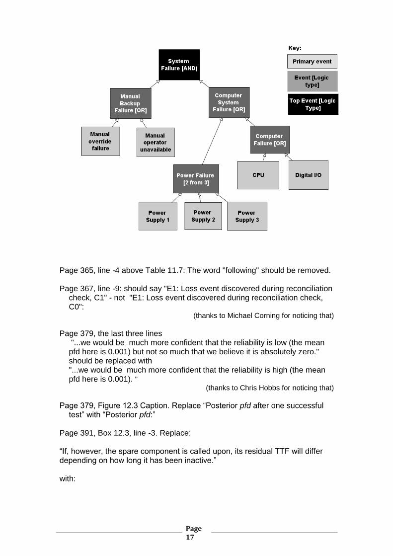
Page 17
Page 365, line -4 above Table 11.7: The word "following" should be removed. Page 367, line -9: should say "E1: Loss event discovered during reconciliation
check, C1" - not "E1: Loss event discovered during reconciliation check, C0":
(thanks to Michael Corning for noticing that)
Page 379, the last three lines
"...we would be much more confident that the reliability is low (the mean pfd here is 0.001) but not so much that we believe it is absolutely zero." should be replaced with "...we would be much more confident that the reliability is high (the mean pfd here is 0.001). "
(thanks to Chris Hobbs for noticing that)
Page 379, Figure 12.3 Caption. Replace “Posterior pfd after one successful
test” with “Posterior pfd:” Page 391, Box 12.3, line -3. Replace: “If, however, the spare component is called upon, its residual TTF will differ depending on how long it has been inactive.” with:
Page 18
“If, however, the spare component is called upon, its residual TTF will differ depending on how long it has been inactive, which is the equivalent operating
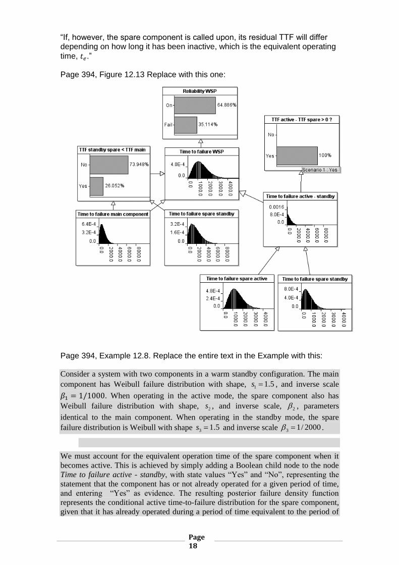
time, 𝑡𝑒.” Page 394, Figure 12.13 Replace with this one:
Page 394, Example 12.8. Replace the entire text in the Example with this:
Consider a system with two components in a warm standby configuration. The main
component has Weibull failure distribution with shape, 1 1.5s , and inverse scale
𝛽1 = 1/1000. When operating in the active mode, the spare component also has
Weibull failure distribution with shape, 2s , and inverse scale, 2 , parameters
identical to the main component. When operating in the standby mode, the spare
failure distribution is Weibull with shape 3 1.5s and inverse scale 3 1/ 2000 .
We must account for the equivalent operation time of the spare component when it
becomes active. This is achieved by simply adding a Boolean child node to the node
Time to failure active - standby, with state values “Yes” and “No”, representing the
statement that the component has or not already operated for a given period of time,
and entering “Yes” as evidence. The resulting posterior failure density function
represents the conditional active time-to-failure distribution for the spare component,
given that it has already operated during a period of time equivalent to the period of
Page 19
operation in standby mode. The resulting BN is depicted in Figure 12.13, with
marginal and conditional distributions superimposed on the graph. The reliability of
the system at a mission time 1000t hours is also shown in the graph in node
Reliability WSP.
The reliability of the WSP system is 0.649 and the MTTF is 1358.
Page 426, sidebar (setting soft evidence). Replace “Cause 1: 1/p1” with
“Cause 2: 1/p1” (thanks to Robbie Heremans for noticing that)
Page 426, Figure 13.22. The table is wrong. It should be replaced with this
one
(thanks to Robbie Heremans for noticing that)
Page 446, Example A.11. Answer should be 10 NOT 30.
(thanks to Dave Palmer for noticing that)
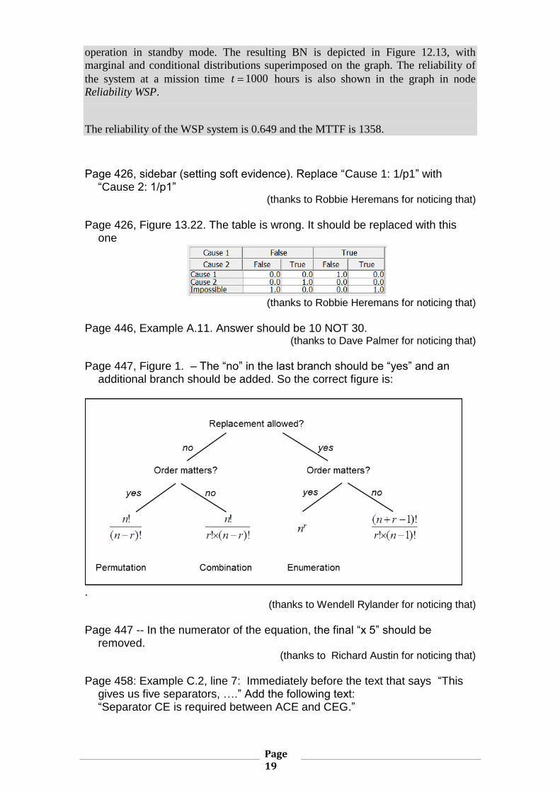
Page 447, Figure 1. – The “no” in the last branch should be “yes” and an
additional branch should be added. So the correct figure is:
.
(thanks to Wendell Rylander for noticing that)
Page 447 -- In the numerator of the equation, the final “x 5” should be
removed. (thanks to Richard Austin for noticing that)
Page 458: Example C.2, line 7: Immediately before the text that says “This
gives us five separators, ….” Add the following text: “Separator CE is required between ACE and CEG.”
Page 20
(thanks to Hashmat Mastan for noticing that)
Page 496 index entry "Bookmakers odds, see Odds" should be replaced with
"Bookmakers odds, 70-71" (the item does not appear currently under Odds)
Page 497 index entry "Discretization, static, 280, 465" should be replaced
with "Discretization, static, 273-280, 465" Page 497 index entry "Discretization, state domain notation, 273" should be
moved to an entry on its own, i.e. "state domain notation, 273" Page 498 index entry "Evidence, likelihood ratio, 122" should be replaced
with "Evidence, likelihood ratio, 125-128, 409-410" Page 499 index entry "Marginalization by variable elimination, 142" should be
replaced with "Marginalization, 58-59, 85-88, 142-144, 450-451" Page 499 index entry "Evidence, likelihood ratio, 122" should be replaced
with "Evidence, likelihood ratio, 125-128, 409-410" Page 500 index entry "node, SPAM filters, 232" should be moved to an entry
on its own, i.e. "SPAM filters, 232" Page 502 index entry “Simpson’s paradox”: add “161-162” after “18, 21-23”.
Also add 161-162 after the subentry “causal model, 22” Back Cover, line -2 "..PowerPoint slides" should be removed. The following
sentence should be added: "A full set of PowerPoint slides is freely available to teachers adopting the book on their course".