Applied Acoustics 15 (1982) 263 274

ERROR INVESTIGATION FOR THE RAY TRACING TECHNIQUE*

A. KULOWSKI~"

Laboratory of Architectural Design, University of Thessaloniki, Thessalonika (Greece)

(Received: 10 August, 1981)

SUMMARY

This paper presents a method o f determining a quantitative measure o f the ray tracing technique error. This error results f rom replacing a wave structure of an acoustical f ield by a grain one. A standard deviation is used as a credibility parameter of the calculation result. Other kinds o f credibility parameters are also considered.

INTRODUCTION

A convenient means of investigating acoustical fields in rooms is the geometrical method. In this method, a wave propagation phenomenon occurring in a limited space is described by the wave reflection rule. Wave phenomena occurring in a field are neglected.

There are two forms of geometrical method currently in use--the image method and the ray tracing technique. The main difference between them arises from a choice of initial wave fronts being traced.

In the image method only those directions are considered which run, after an assumed number of reflections, to an observation place. Sound intensity is calculated along those directions. If the place of observation is assumed to be a point, the image method is an exact representation of a wave propagation from a source to that point. In such a case, sound intensity at an observation point is of deterministic value.

In the tracing technique, when an omnidirectional sound source is being

* Part of this work was presented at the First Meeting of the Hellenic Acoustical Society in Volos, Greece, In June, 1980. t On leave from the Institute of Telecommunication, Technical University of Gdafisk, 80-952 Gdafisk, Majakowskiego ll/12, Poland.

263 Applied Acoustics 0003-682X/82/0015-0263/$02-75 © Applied Science Publishers Ltd, England, 1982 Printed in Great Britain

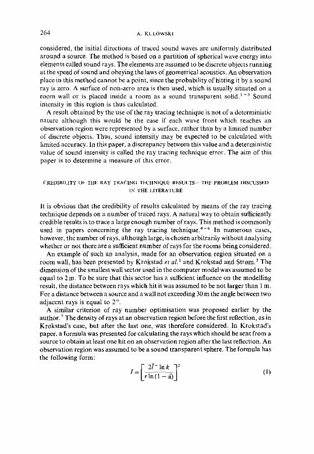
264 A. KULOWSKI

considered, the initial directions of traced sound waves are uniformly distributed around a source. The method is based on a partition of spherical wave energy into elements called sound rays. The elements are assumed to be discrete objects running at the speed of sound and obeying the laws of geometrical acoustics. An observation place in this method cannot be a point, since the probability of hitting it by a sound ray is zero. A surface of non-zero area is then used, which is usually situated on a room wall or is placed inside a room as a sound transparent solid. ~-3 Sound intensity in this region is thus calculated.

A result obtained by the use of the ray tracing technique is not of a deterministic nature although this would be the case if each wave front which reaches an observation region were represented by a surface, rather than by a limited number of discrete objects. Thus, sound intensity may be expected to be calculated with limited accuracy. In this paper, a discrepancy between this value and a deterministic value of sound intensity is called the ray tracing technique error. The aim of this paper is to determine a measure of this error.

CREDIBILITY OF THE RAY TRACING TECHNIQUE RESULTS--THE PROBLEM DISCUSSED

IN THE LITERATURE

It is obvious that the credibility of results calculated by means of the ray tracing technique depends on a number of traced rays. A natural way to obtain sufficiently credible results is to trace a large enough number of rays. This method is commonly used in papers concerning the ray tracing technique. 4-6 In numerous cases, however, the number of rays, although large, is chosen arbitrarily without analysing whether or not there are a sufficient number of rays for the rooms being considered.

An example of such an analysis, made for an observation region situated on a room wall, has been presented by Krokstad et al.1 and Krokstad and Strom. 3 The dimension of the smallest wall sector used in the computer model was assumed to be equal to 2 m. To be sure that this sector has a sufficient influence on the modelling result, the distance between rays which hit it was assumed to be not larger than 1 m. For a distance between a source and awall not exceeding 30 m the angle between two adjacent rays is equal to 2 °.

A similar criterion of ray number optimisation was proposed earlier by the author, v The density of rays at an observation region before the first reflection, as in Krokstad's case, but after the last one, was therefore considered. In Krokstad's paper, a formula was presented for calculating the rays which should be sent from a source to obtain at least one hit on an observation region after the last reflection. An observation region was assumed to be a sound transparent sphere. The formula has the following form:

i=ir2-[-ln k ]2 mTi-~jJ (i)

ERROR INVESTIGATION FOR THE RAY TRACING TECHNIQUE 265

where I = number of rays sent from the source, T= mean free path, k = factor of energy decay range where each ray is being traced (for example, k = 1 0 6 corresponds to 60dB), r = radius of the observation sphere and c~ = mean sound absorption coefficient.

Another method of checking the credibility of results is an anlysis not of ray numbers, but of the results themselves. In this method, result fluctuations are investigated and are determined as a difference between two forms of result which are obtained in two successive stages of modelling. Fluctuations arise from the statistical nature of the ray tracing t¢chnique. Calculations are continued until the magnitude of such fluctuations decreases below an assumed value. Lamoral and Sauvet-Goichon 8 proposed investigating fluctuations by comparing the results obtained with two ray populations which differ twice. Mathiez and Santon 4 investigated fluctuations not directly, but by testing a result repeatability. For this purpose, the calculations have been repeated with another ray population of the same magnitude.

The methods described permit one to determine an appropriate number of rays for a particular case, according to a chosen criterion. Although, in general, such numbers of rays differ between different rooms, the credibilities of the results obtained may be treated as comparative. Credibility should, however, be considered here merely as a qualitative term, as none of the discussed methods make possible the determination of the magnitude of the ray tracing technique error.

MODEL DESCRIPTION

The form of ray tracing technique considered here is that in which, of the whole population of rays, only those which penetrate a sphere of given radius and centre position compose a sound decay curve. 2'4'9'1° Because of the limitations of a computer memory space, the time axis of a curve is quantised. The graphical form of the calculations result is then a histogram.

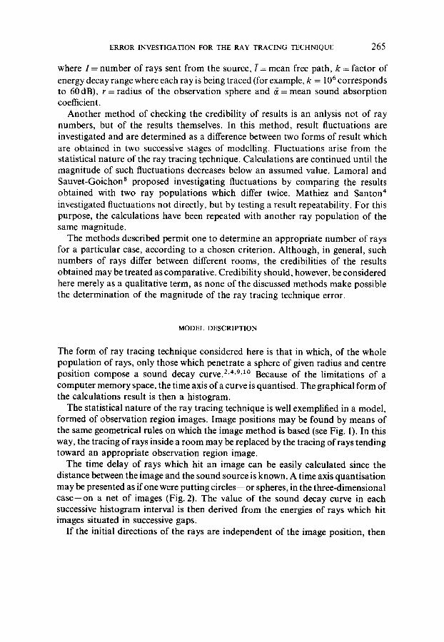
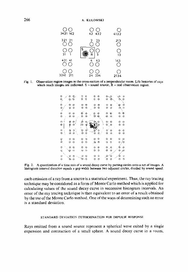
The statistical nature of the ray tracing technique is well exemplified in a model, formed of observation region images. Image positions may be found by means of the same geometrical rules on which the image method is based (see Fig. 1). In this way, the tracing of rays inside a room may be replaced by the tracing of rays tending toward an appropriate observation region image.

The time delay of rays which hit an image can be easily calculated since the distance between the image and the sound source is known. A time axis quantisation may be presented as if one were putting circles--or spheres, in the three-dimensional case--on a net of images (Fig. 2). The value of the sound decay curve in each successive histogram interval is then derived from the energies of rays which hit images situated in successive gaps.

If the initial directions of the rays are independent of the image position, then

2 6 6 A. K U L O W S K I

F i g . 1.

O 0 O 0 0 3 4 2 1 142 4 2 4 3 2 4 1 3 2

3 2 1 21 2 2 3 2 1 3

O 0 O 0 0 O 0 0 31 I 3 13

4 3 1 41 4 4 3 1 4 3

O 0 O 0 0 O 0 O 0 0

3 2 4 1 211 2 4 2 3 4 2 1 3 4

Observation region images in the cross-section o f a p e r p e n d i c u l a r r o o m . Life histories of rays which reach images are indicated. S = sound source; R = real observation region.

0 j "

0 ,/ 0 ,/ / 0 / 0 /'

o/ 0

o 0

o q

o o

0 0 0 0

0 o O O 0 0 o 0 0 0 0 0 0 0 o 0

0 o ~ 0 0 0 o 0 o , o o o o ~ 0 0 o

o ~ o o 0 o ' 0 0 0 o ' 0 o

0 0 O o 0 o o 0 0 o 0 o O 0 0 0

0 0 0 0 0 0 0 0 "~() 0 0 0

0 - 0 0 0 " ~ 0 - 0

0

0 0

0 0

0 o o//o ,d o

o o 0 0 0

~ ° o x\

0 © O

o 0

o o

0 0 0 0 / ' / 0

o o zo~o o o o o o o

F i g . 2. A quantisation o f a time axis o f a sound decay curve by putting circles o n t o a n e t o f images. A histogram interval duration equals a gap width between two adjacent circles, divided by sound speed.

each emission of a ray from a source is a statistical experiment. Thus, the ray tracing technique may be considered as a form of Monte Carlo method which is applied for calculating values of the sound decay curve in successive histogram intervals. An error of the ray tracing technique is then equivalent to an error of a result obtained by the use of the Monte Carlo method. One of the ways of determining such an error is a standard deviation.

STANDARD DEVIATION DETERMINATION FOR IMPULSE RESPONSE

Rays emitted from a sound source represent a spherical wave exited by a single expansion and contraction of a small sphere. A sound decay curve in a room,

E R R O R INVESTIGATION FOR THE RAY T R A C I N G T E C H N I Q U E 267

calculated by means of the ray tracing technique, may then be interpreted as its impulse response.

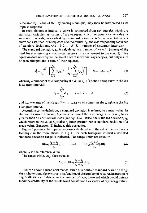
In each histogram interval a curve is composed from ray energies which are statistical variables. A scatter of ray energies, which compose a curve value in successive intervals, is described by a standard deviation. A full representation of a curve consists, then, of a sequence of curve values, e k, and a corresponding sequence of standard deviations, $ k ( k - ~ 1 , 2 . . . . . K; K = number of histogram intervals).

The standard deviation, Sk, is calculated in a number of ways. 11 Because of the need for economising in computer memory, it is convenient to use eqn. (2). This equation does not require the use of a set of individual ray energies, but only a sum of such energies and a sum of their squares.

nk nk

2 n k ( e l , k ) 2 - - el, k k = 1,2, K (2) S k - - n k - - 1 " " " '

i = 1 i = 1

where n k = number of rays composing the value, gk, of a sound decay curve in the kth histogram interval:

nk

e k = ) ' , e i , k k = l, 2 . . . . . K (3)

i = 1

and el, k = energy of the ith r a y ( / = l . . . . . r/k) which comprises the gk value in the kth

histogram interval. According to the definition, a standard deviation is referred to a mean value. In

the case discussed, however, E k equals the sum of the rays' energies, i.e. it is/7 k times greater than an arithmetical mean (see eqn. (3)). Hence, the standard deviation, Sk,

which refers to the value E k is also n k times greater than a standard deviation of a mean value. Equation (2) includes this correction.

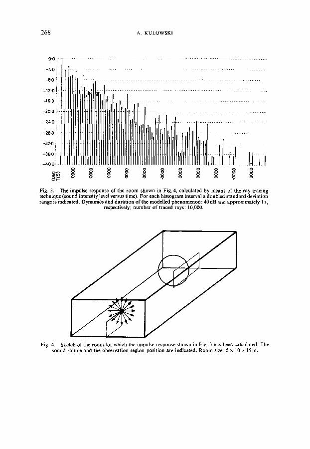
Figure 3 presents the impulse response calculated with the aid of the ray tracing technique in the room shown in Fig. 4. For each histogram interval a doubled standard deviation range is indicated. The range limits are equal to:

10 log ek + sk (dB) and 10 log 6k + Sk (dB) (4) 13 0 6 0

where 6 o is the reference value. The range width, Aek, then equals:

Ae k = l0 log 6k + sk (dB) (5) •k - - Sk

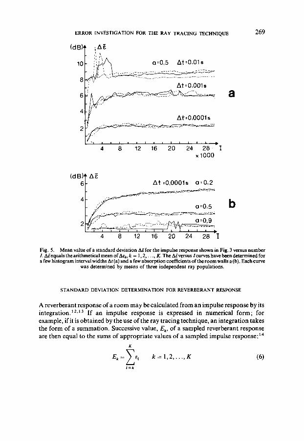
Figure 5 shows a mean arithmetical value of a doubled~standard deviation range for a whole sound decay curve, as a function of the number of rays. An inspection of Fig. 5 allows one to determine the number of rays, to exceed which would detract from the credibility of the results when considered as a scatter of ray energy values.

268 A. KULOWSKI

0'0 !-

-4"0 1

- °il -12"0

-16.0 i--

-20"0 i- !

-24"O i--,

_28.0!1

-32"0 1

-36.o ;

~o.oi

9 ~ oO g oO

• O o

Fig. 3. The impulse response of the room shown in Fig. 4, calculated by means of the ray tracing technique (sound intensity level versus time). For each histogram interval a doubled standard deviation range is indicated. Dynamics and duration of the modelled phenomenon: 40 dB and approximately I s,

respectively; number of traced rays: 10,000.

Fig. 4. Sketch of the room for which the impulse response shown in Fig. 3 has been calculated• The sound source and the observation region position are indicated. Room size: 5 x 10 x 15 m.

ERROR INVESTIGATION FOR TIlE RAY TRACING TECHNIQUE

(dB) T ii ~e

At : 0,001 s

4

2

Af :0 ,0001s

-' ' ' ; ' 1 ; ' . . . . ' 4 24 28 " I

x 1000

a

269

(dB) ' 6

4

2

AE At:O,OOOls a=0,2

a:O,5

,, a:O,9

I I I I I I I I I I I i J ,

4 8 12 16 20 24 28 I

b

Fig. 5. Mean value of a standard deviation Ai for the impulse response shown in Fig. 3 versus number 1. Agequals the arithmetical mean of Aek, k = 1 ,2 , . . . , K. The Agversus /curves have been determined for a few histogram interval widths At (a) and a few absorption coefficients of the room walls ,, (b). Each curve

was determined by means of three independent ray populations.

STANDARD DEVIATION DETERMINATION FOR REVERBERANT RESPONSE

A reverberant response of a room may be calculated from an impulse response by its integration. 12,13 I f an impulse response is expressed in numerical form; for example, if it is obtained by the use of the ray tracing technique, an integration takes the form of a summation. Successive value, Ek, of a sampled reverberant response are then equal to the sums of appropriate values of a sampled impulse response: 14

K

) ' e t k = 1,2 . . . . . K (6) E~ l = k

270 A. KULOWSKI

" i~h

Q

Iss"ili,~,.~ 1 :m,

-. . . . , . , ; : ; . . . . . . . . . . . .

iii'??!<i.i i ii -,.,,

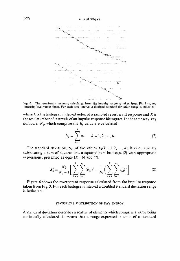
Fig. 6. The reverberant response calculated from the impulse response taken from Fig. 3 (sound intensity level versus time). For each time interval a doubled standard deviation range is indicated.

where k is the histogram interval index of a sampled reverberant response and K is the total number of intervals of an impulse response histogram. In the same way, ray numbers, Nk, which comprise the E k value are calculated:

K

N k= ~ n l k = l , 2 . . . . . K (7)

l = k

The standard deviation, Sk, of the values Ek(k = 1 ,2 , . . . , K) is calculated by substituting a sum of squares and a squared sum into eqn. (2) with appropriate expressions, presented as eqns (3), (6) and (7).

K n k K n k

l = k i = 1 l = k i = 1

(8)

Figure 6 shows the reverberant response calculated from the impulse response taken from Fig. 3. For each histogram interval a doubled standard deviation range is indicated.

STATISTICAL DISTRIBUTION OF RAY ENERGY

A standard deviation describes a scatter of elements which comprise a value being statistically calculated. It means that a range expressed in units o f a standard

ERROR INVESTIGATION FOR THE RAY TRACING TECHNIQUE 271

deviation may be determined in which a given percentage of elements is contained. To calculate this range, a statistical distribution of elements should be known. For example, in the case of Gaussian distribution, 68,239 elements are contained in the range of 2s width, 95.45 per cent-- in the range of 4s width, etc., where s is the standard deviation.11 A range width may then be interpreted as a measure of an error being made when a value is being statistically determined.

A sound decay curve in successive histogram intervals is composed of energies of those rays which penetrate observation region images situated in successive gaps of the image model. Assuming that the sound absorption in the air is neglected, the rays' energy, which is emitted in the ruth direction, penetrating an ith order image, may be expressed as follows:

ea = eo(1 - ~Xm,1)(1 - - ~ m , 2 ) " " ' (1 - O~m,i) (9)

where ea, e 0 are actual and initial energy of a ray, respectively, ~tm, 1 . . . . . Ctm, i are sound absorption coefficients of walls, from which a ray would be reflected on its way to a real observation region and i is the number of reflections.

The statistical distribution of ray energies may be determined by a presumption of possible values of the product (1 - gm.~)'"" (1 - gin,i) or, equivalently, by an analysis of the life histories of rays. This kind of analysis may easily be made by an investigation of image indexes in a gap corresponding to a histogram interval being analysed (see Figs I and 2). An inspection of Figs 1 and 2 shows, however, that such an analysis may be made only in a specific case. In a general case there is no way of performing it since both images net and there is no fixed gap width.

INVESTIGATION OF FLUCTUATIONS IN FUNCTION OF NUMBER OF RAYS

The use of a standard deviation as a result credibility parameter is convenient for credibility investigation because it helps to control a result in a continuous manner, i.e. ray by ray. For large ray populations, however, a standard deviation depends weakly on a traced ray number (Fig. 5).

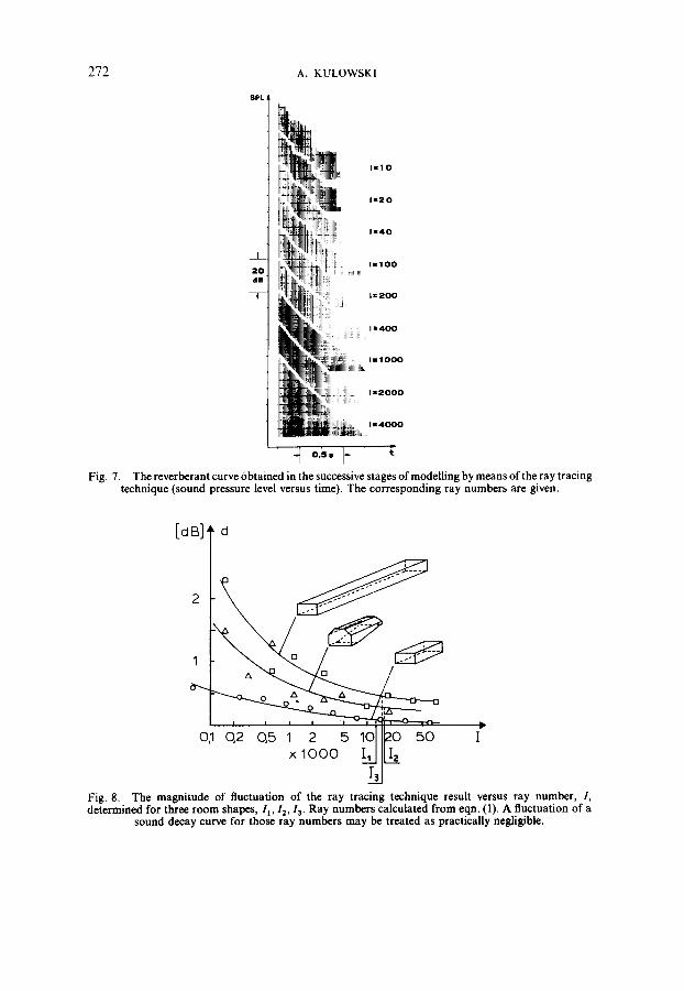
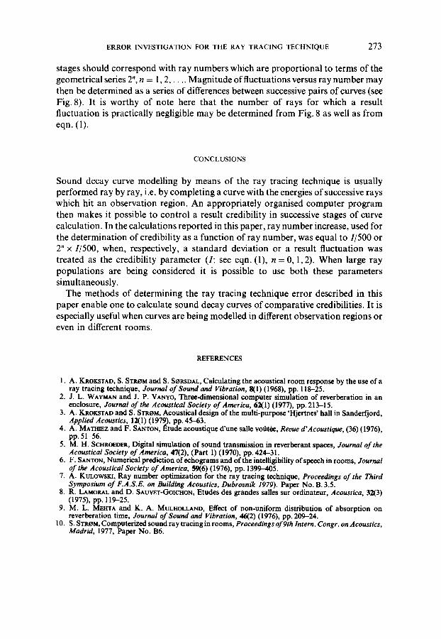
Another situation occurs when the magnitude of result fluctuations is used as a credibility parameter. In this paper, the magnitude of fluctuations is determined as an arithmetical mean of absolute differences between two sound decay curves obtained at two successive stages of calculation (see Fig. 7). A noticeable influence of ray number on a curve shape shows that the magnitude of fluctuations, when used as a credibility parameter, may be expected to be more efficient than a standard deviation, especially for large ray populations. On the other hand, the magnitude of fluctuations, when considered as a function of ray number, may only be determined for a fixed number of rays. For example, Lamoral and Sauvet-Goichon 8 considered two sound decay curves, calculated for ray numbers differing twice. According to this, to investigate fluctuations as a function of ray number, successive calculation

272 A. KULOWSKI

$PL

2 0 dB

7 - -

~llii *II o

J]tt~ I I 2 0

l~iliL~i ,.,,o it~i ....

. ]]i!iIiii , ,.,oo lll!~;lillill;ii!i;iiild~ 1

i!ii!;i!![!!ii!i:!::i:i 1 = 2 0 0

:li!Hi:i,~: !!~!!!!i~!!!i!!iii:ii!ii~ I B 4 0 0 ~%;i~iiiiiiiiiiiiiiiiiiiill;,,, i

ii~'ii~iiliiiiiiiii~' I I 1 0 0 0 :iiiiijliiiiillillii~iiiiii!]i,,,

o,5. I-

1 1 2 0 0 0

I I 4 0 0 0

Fig. 7. The reverberant curve obtained in the successive stages of modelling by means of the ray tracing technique (sound pressure level versus time). The corresponding ray numbers are given.

[d B]' d

1 A [] o

111

50 I

× 1 o o o III, N

Fig. 8. The magnitude of fluctuation of the ray tracing technique result versus ray number, I, determined for three room shapes, 11,12,13. Ray numbers calculated from eqn. (1). A fluctuation of a

sound decay curve for those ray numbers may be treated as practically negligible.

ERROR INVESTIGATION FOR THE RAY TRACING TECHNIQUE 273

stages should co r re spond with ray numbers which are p r o p o r t i o n a l to terms o f the geometr ica l series 2", n = 1,2 . . . . . M a g n i t u d e of f luctuat ions versus ray number m a y then be de te rmined as a series o f differences between successive pairs o f curves (see Fig. 8). I t is wor thy o f note here tha t the number o f rays for which a resul t f luctuat ion is prac t ica l ly negligible m a y be de te rmined f rom Fig. 8 as well as f rom eqn. (1).

CONCLUSIONS

Sound decay curve model l ing by means of the ray t rac ing technique is usual ly pe r fo rmed ray by ray, i.e. by comple t ing a curve with the energies o f successive rays which hit an observa t ion region. A n app rop r i a t e ly organised compute r p r o g r a m then makes it poss ible to con t ro l a result c redibi l i ty in successive stages o f curve calcula t ion. In the ca lcula t ions r epor t ed in this paper , r ay number increase, used for the de te rmina t ion o f credibi l i ty as a funct ion o f ray number , was equal to •/500 or 2" x •/500, when, respectively, a s t anda rd devia t ion or a result f luctuat ion was t rea ted as the credibi l i ty p a r a m e t e r ( I : see eqn. (1), n = 0, 1,2). When large ray popu la t ions are being cons idered it is poss ible to use bo th these pa rame te r s s imul taneously .

The me thods o f de te rmin ing the ray t rac ing technique e r ror descr ibed in this paper enable one to calculate sound decay curves o f compara t ive credibil i t ies. I t is especial ly useful when curves are being model led in different observa t ion regions or even in different rooms.

REFERENCES

1. A. KROKSTAD, S. STROM and S. SORSDAL, Calculating the acoustical room response by the use of a ray tracing technique, Journal of Soand and Vibration, 8(1) (1968), pp. 118-25.

2. J. L. W^YMAN and J. P. VANYO, Three-dimensional computer simulation of reverberation in an enclosure, Journal of the Acoustical Society of America, 62(1) (1977), pp. 213-15.

3. A. KROKSTAD and S. STRUM, Acoustical design of the multi-purpose 'Hjertnes' hall in Sanderfjord, Applied Acoustics, 12(1) (1979), pp. 45-63.

4. A. MATmEZ and F. SANTOS, Etude acoustique d'une salle vofit~e, Revue d'Acoustique, (36) (1976), pp. 51-56.

5. M. H. SCHRO~DeR, Digital simulation of sound transmission in reverberant spaces, Journal of the Acoustical Society of America, 47(2), (Part 1) (1970), pp. 424-31.

6. F. SANTON, Numerical prediction ofechograms and of the intelligibility of speech in rooms, Journal of the Acoustical Society of America, 59(6) (1976), pp. 1399--405.

7. A. KULOWSKI, Ray number optimization for the ray tracing technique, Proceedings of the Third Symposium of F.A.S.E. on Building Acoustics, Dubrovnik 1979). Paper No. B. 3.5.

8. R. LAMORAL and D. SAUVET-GOICHON, Etudes des grandes salles sur ordinateur, Acoustica, 32(3) (1975), pp. 119-25.

9. M. L. MEHTA and K. A. MULHOLLAND, Effect of non-uniform distribution of absorption on reverberation time, Journal of Sound and Vibration, 46(2) (1976), pp. 209-24.

10. S. STROM, Computerized sound ray tracing in rooms, Proceedings of 9th Intern. Congr. on Acoustics, Madrid, 1977, Paper No. B6.

274 A. KULOWSKI

11. R. ZmUNSrd, Metody Monte Carlo, WNT, Warszawa 1970. (In Polish). 12. M. R. SCHrtOEDEI~, New method of measuring reverberation time, Journal of the Acoustical Society

of America, 37(3) (1965), pp. 409-12. 13. L. CP, EMER and H. A. MOLLER, Die wissenshaftlichen Grundlagen der Raumakustik, I, (2), S. Hirzel

Verlag, 1978. 14. A. KULOWSK1, Relationship between impulse response and other types of room acoustical responses,

Applied Acoustics 15(1) (1981), pp. 3-10.