Error discounting 1

Running head: ERROR DISCOUNTING

Error Discounting in Probabilistic Category Learning

Stewart Craig and Stephan Lewandowsky

School of Psychology

The University of Western Australia

Daniel R. Little

The University of Western Australia, Indiana University, and The University of Melbourne

Keywords: categorization, learning, error, relevance shifts

School of Psychology

University of Western Australia

Crawley, W.A. 6009, AUSTRALIA

lewan@psy.uwa.edu.au

URL: http://www.cogsciwa.com/

Error discounting 2

Abstract

Some current theories of probabilistic categorization assume that people gradually

attenuate their learning in response to unavoidable error. However, existing evidence for

this error discounting is sparse and open to alternative interpretations. We report two

probabilistic-categorization experiments that investigated error discounting by shifting

feedback probabilities to new values after different amounts of training. In both

experiments, responding gradually became less responsive to errors, and learning was

slowed for some time after the feedback shift. Both results are indicative of error

discounting. Quantitative modeling of the data revealed that adding a mechanism for

error discounting significantly improved the fits of an exemplar-based and a rule-based

associative learning model, as well as of a recency-based model of categorization. We

conclude that error discounting is an important component of probabilistic learning.

Error discounting 3

Error Discounting in Probabilistic Category Learning

Throughout daily life, people make decisions based on uncertain cues that predict

multiple outcomes: Doctors make diagnoses based on symptoms that are indicative of

several potential diseases; dark clouds do not always bring rain, yet an overcast day is

more likely to be associated with precipitation than sunshine; and despite injuries, trades,

and home-field advantages, we learn to predict which teams are likely to win on the

weekend. Accurate prediction requires learning probabilistic relationships between cues

and uncertain outcomes (Kruschke & Johansen, 1999). Probabilistic categorization is one

form of probability learning in which the to-be-predicted outcomes are discrete categorical

values. Unlike its deterministic counterpart, in probabilistic categorization the same

stimuli belong to multiple categories albeit with differing probabilities. In consequence,

the same response to an identical stimulus can be reinforced as either correct or incorrect

on a probabilistic basis (Kruschke & Johansen, 1999). This corrective feedback is often

believed to drive category learning (Gluck & Bower, 1988a, 1988b; Rumelhart, Hinton, &

Williams, 1986).

In deterministic category learning, people often perform sufficiently well to eliminate

error completely. In probabilistic categorization, by contrast, avoiding errors and

achieving perfect accuracy is by definition impossible. On that basis, Kruschke and

Johansen (1999) proposed that during probabilistic categorization, people may eventually

accept a certain level of unavoidable error and progressively slow their learning, a

phenomenon known as error discounting. Kruschke and Johansen (1999) instantiated

error discounting within a computational model, called RASHNL (Rapid Attention SHifts

’N’ Learning). RASHNL includes an error discounting mechanism based on an

“annealing” process, which works by reducing learning rates across time (e.g., Amari,

1967; Heskes & Kappen, 1991; Murata, Kawanabe, Ziehe, Muller, & Amari, 2002). This

decline in learning rates causes a gradual decrease in the rate at which RASHNL updates

Error discounting 4

associations. Thus, as learning progresses, errors are increasingly discounted because they

contribute less and less to learning. The annealed learning provides the model with

various advantages over a fixed learning rate: For example, annealing allows for large

response shifts early in training, to quickly adapt to the environment, while the slowing of

learning later in training permits the fine-tuning of probabilistic responding (e.g., Amari,

1967; Heskes & Kappen, 1991; Murata et al., 2002).

This article critically examines the notion of error discounting and seeks supporting

evidence for its operation in probabilistic categorization. We start by examining existing

evidence for discounting and find it to be surprisingly sparse. We next present two

probabilistic categorization experiments in which the reinforcement probabilities for all

stimuli were shifted during training, with the abruptness and timing of the shift varying

between experiments and conditions. We present two forms of analysis to confirm the

presence of error discounting. First, we examine decisional-recency effects in

categorization. The analysis of decisional recency, as developed by Jones, Love, and

Maddox (2006), pinpoints how people adjust their behavior in response to feedback from

the immediately preceding trial. Using an extension of Jones et al. (2006)’s original

analysis, we show that participants gradually come to ignore error feedback when making

category decisions, and their sensitivity to feedback is only gradually restored after

reinforcement probabilities change. Second, we applied four models of categorization to

the results: An exemplar model without an associative-learning mechanism that bases

decisions on a similarity comparison to all previously stored exemplars (the Generalized

Context Model, GCM; Nosofsky, 1986), a model that utilizes only recency information

(the Memory and Context model, MAC; Stewart, Brown, & Chater, 2002), a second

exemplar model based on associative learning (RASHNL; Kruschke & Johansen, 1999),

and a rule-based model that also included associative learning (derived from the hybrid

Attention to Rules and Instances in a Unified Model, ATRIUM; Erickson & Kruschke,

Error discounting 5

1998, 2002). We find that only the associative-learning models provide an accurate

account of the data. Additionally, the MAC, RASHNL, and ATRIUM models provide a

significantly better account if they incorporate an error-discounting mechanism. We

conclude that error discounting deserves to be given a prominent theoretical role in

probabilistic categorization.

Error Discounting in Probabilistic Environments

Examination of the applied literature on performance in complex environments

indicates that ignoring unreliable cues is a common risk in industrial settings (Lorenz &

Parasuraman, 2007; Moray, 2007) and aviation (Wickens, 2007). However, the existing

evidence for error discounting is equivocal. Empirical support for error discounting

involves the finding that the delayed introduction of cues reduces their utilization (Edgell,

1983; Edgell & Morrissey, 1987). If cues suddenly become relevant after an initial period

of non-relevance, people use them less than equivalent cues that were relevant from the

outset. That is, people fail to notice a change in the environment and fail to learn (much)

about a highly relevant but new cue (Kruschke & Johansen, 1999). Although this finding

is suggestive of error discounting, other explanations, such as those for conventional

blocking (Kamin, 1969; Rescorla & Wagner, 1972), cannot be ruled out. Blocking occurs

when a previously learned association between a cue, A, and an outcome, X, prevents

learning of a new association between a second cue, B, and X, when trained in the

presence of A (Kruschke & Blair, 2000). For example, after learning to associate a beep

with an electric shock, further training with the conjunction of (the same) beep and a

(novel) light (i.e., both the beep and the light now predict the ensuing shock) does not

lead to any learning about the light. The light on its own will show little if any evidence

of having been learned on a final test. Newly-relevant cues in probabilistic learning may

be under-utilized because learning about the new cue may have been blocked by the

Error discounting 6

association between the already-predictive cue(s) and the outcome. It is preferable to seek

evidence for error discounting in situations in which there is only one stimulus dimension

present: with a single cue, blocking cannot occur. The single-cue approach recognizes that

if error discounting is present, people should be insensitive to shifts in reinforcement

probabilities. For example, if a stimulus is initially placed in category A with 80%

probability, and this suddenly shifts to 20% at some point during learning, error

discounting implies that people might continue to predominantly assign that stimulus to

category A, at least for some time.

Relevance Shifts in Probabilistic Environments

Research on the effects of shifts in reinforcement probabilities dates back several

decades (Estes, 1984; Estes & Straughn, 1954; M. P. Friedman et al., 1964; Yelen & Yelen,

1969). However, upon closer inspection, those data turn out to be either ambivalent or of

little relevance to the error-discounting notion. In a series of early studies (e.g., Estes &

Straughn, 1954; M. P. Friedman et al., 1964; Yelen & Yelen, 1969) participants learned to

predict which of two lights would be illuminated on the next trial. The actual

probabilities with which the lights were illuminated differed from chance, and by

associating the actual outcome (identity of the illuminated light) with their prediction,

people’s responses gradually came to track the actual event probabilities. Most relevant

here is the fact that in all studies those probabilities changed during the experiment. For

example, in the study by Yelen and Yelen (1969), one light might be illuminated on 90%

of the first 100 trials (and the other light during the remaining 10%), with those

probabilities suddenly reversing for the next 100 trials. In virtually all cases, participants

were found to adapt to those changes with remarkable speed. At first glance, this outcome

might seem to compromise the notion of error discounting. Upon closer inspection,

however, the data arguably have little bearing on probabilistic categorization processes

Error discounting 7

because people never associated distinct outcomes to different stimuli: The only

“stimulus” in those early studies was the signal that denoted the beginning of a trial, and

consequently any observed learning did not necessarily involve the formation of

associations between stimuli and outcomes but simple awareness of base-rates of

reinforcement. The data of Estes and Straughn (1954), M. P. Friedman et al. (1964), and

Yelen and Yelen (1969) thus confirm that people remain sensitive to base-rates even after

more than 1,000 trials with varying probabilities (M. P. Friedman et al., 1964); however,

they tell us little about error discounting.

More recently, in a closer analogue to probabilistic categorization, Estes (1984)

asked participants to choose between two alternatives on each trial. Each alternative, in

turn, was associated with two outcomes (success or failure) that were reinforced with some

varying probability. For one of the alternatives, the probability of success remained

constant at .5 throughout. For the other alternative, the probability of success increased

and decreased throughout training following a sine pattern. The results were intriguing:

On the one hand, Estes found that participants were generally aware of the changing

probability structure for one of the outcomes and responded accordingly (i.e., following

the cyclical sine pattern, preferring that alternative whenever its probability of success

exceeded .5 and rejecting it whenever it fell below .5). On the other hand, during a final

transfer block involving a uniform probability of success of .5 for both alternatives, people

persisted with the cyclical pattern and showed little evidence of adaptation.

On balance, the existing data involving relevance shifts are, at best, ambivalent with

respect to error discounting. The study that most closely resembled probabilistic

categorization (Estes, 1984), simultaneously found evidence both for people’s ability to

track changing probabilities and against their ability to adapt after prolonged training.

The latter outcome is suggestive of error discounting but remains inconclusive.

Error discounting 8

Present Experiments

The present experiments used a single, quasi-continuous cue that could take on four

values; each value was probabilistically associated with two categories. The use of a single

cue precluded the possibility of blocking. The principal manipulation in the experiments

involved switching the reinforcement probabilities of the two categories part-way through

training. Between experiments, we varied the rate at which the reinforcement probabilities

were shifted, which was either sudden (Experiment 1) or gradual (Experiment 2). If the

reinforcement probabilities are shifted gradually, the increase in error at any point during

the shift is limited. That limited increase, in turn, might be more likely to be discounted.

By contrast, a sudden shift in the reinforcement contingencies would lead to a large

increase in the error signal, potentially alerting participants to the new environment.

Within each experiment, we varied the point at which the shift occurred.

Experiment 1

The first experiment used a single sudden shift in reinforcement. Depending on

condition, the shift occurred either early, near the middle, or late in the training sequence.

Method

Participants. Sixty-four members of the University of Western Australia campus

community participated in the experiment. Participants were randomly assigned to one of

three conditions; early, mid, or late. The number of participants in the three conditions

was 21, 21, and 22, for the early, mid, and late conditions respectively. Participants

received either course credit or A$10 remuneration.

Stimuli and apparatus. The experiment was controlled by a Windows computer

using a MATLAB program created with the aid of the Psychophysics toolbox (Brainard,

1997; Pelli, 1991). The task was a single-cue binary choice task that required participants

Error discounting 9

to classify a set of 4 unique items into one of two categories, A or B. To control for

potential idiosyncrasies of the stimuli, two different types of stimuli were used, either

squares of varying size, or circles with a radial line at varying angles. Within each

condition, participants were randomly assigned to stimulus type. For the squares, the 4

training items were of linearly increasing sizes of 44, 66, 88, and 110 mm edge length. The

circles were all approximately 115 mm in diameter. The radial line within the circle was

presented at increasing angles of 36, 72, 108, and 144 degrees (measured from the

vertical). For some participants the radial line was presented in the left hemisphere of the

circle whereas for others it was shown in the right hemisphere.

Stimuli were presented in black on a white background. The category membership

of each stimulus was determined on a probabilistic basis, with the probability of an item

belonging to category A at the outset of training equaling .2, .4, .6, and .8 in increasing

order of size (or angle), respectively. Category B probabilities were 1− P (A). Part-way

through the experiment, those probabilities were shifted instantaneously, such that the

probability of the items belonging to category A changed to .8, .6, .4, and .2. Category B

probabilities also shifted, and remained at 1− P (A). The point at which this shift

occurred varied between conditions: The shift occurred at the beginning of training block

2, 11, or 16 for the early, mid, and late conditions, respectively.

Procedure. Each trial commenced with a fixation symbol (“+”) in the center of the

screen for 500 ms. The “+” was replaced by the stimulus, which was presented in the

center of the screen along with the response options (i.e., Category A or Category B)

underneath. The stimulus and response options remained visible until a response was

made. Responses were made by pressing the “F” or “J” keys. Mappings of the two

response keys to categories (A or B) were randomly determined for each participant. After

each response, feedback (“CORRECT” or “WRONG”) was presented on the screen, below

the item, for 1,300 ms.

Error discounting 10

Items were randomly presented in blocks of 40 trials, with each stimulus presented

10 times per block. Participants were trained for 18 blocks altogether. Self-timed breaks,

lasting a minimum of 30 seconds, were presented after every four blocks.

Results and Discussion

In probabilistic categorization, above-chance performance can involve one of two

primary behaviors, known as probability-matching and maximizing, respectively (Fantino

& Esfandiari, 2002; Shanks, Tunney, & McCarthy, 2002). Probability matching is said to

occur if people place items into particular categories with a frequency approximately

equivalent to the probability of reinforcement: For example, if stimulus j is assigned to

category A on 80% of all trials, then people probability match if they respond A with

probability .8. By contrast, maximizing is said to occur if people always place an item into

the category to which it is most likely to belong. Thus, for the above item j, maximizing

implies that instead of responding with A 80% of the time, people would respond with A

on all trials. In most situations, people tend to probability match rather than maximize

(Fantino & Esfandiari, 2002; Shanks et al., 2002), although people’s performance may lie

anywhere along that continuum.

To characterize performance, we computed probability-matching (PM) scores for the

participants’ mean responses during the last pre-shift block(s); Block 1 for the early

condition, Blocks 9 and 10 for the mid condition, and Blocks 14 and 15 for the late

condition. PM scores were computed based on the following formula:

PMij = (Ri(A|j)− P (A|j)) ∗ SIj , (1)

where P (A|j) is the training probability for item j, and Ri(A|j) is the probability of

participant i responding with category A in response to item j. SIj is a sign indicator for

item j, such that SIj = −1 if P (A|j) < .5 and SIj = 1 if P (A|j) > .5 (D. Friedman &

Error discounting 11

Massaro, 1998; Little & Lewandowsky, 2009b). Each participant’s PM score was based on

the average score across the four items.

For ease of interpretation, the PM scores were then transformed to a scale ranging

from 0 (chance responding) to 1 (full maximizing). For the present probability structure, a

score of .4 indicates perfect probability matching. (Scores below 0 indicate reversed

responding.) To ensure that only participants who learned the probability structures were

included, participants with PM scores of less than 0 were removed from consideration

(N = 3, 4, and 5 in the early, mid, and late conditions, respectively).

Trials with a response time (RT) of less than 150 ms or an RT more than 4 SDs

above the participant’s mean RT were removed from the analysis. Additionally, any

participant who scored more than 10% of all RTs beyond these cutoffs was excluded from

further analysis. Based on these criteria, an additional 3 participants were removed from

each of the early, mid, and late conditions.

After the removal of all outliers, the mean PM scores for the remaining participants

were 0.44 (SD = 0.33), 0.58 (SD = 0.27), and 0.50 (SD = 0.26), for the early, mid, and

late conditions, respectively. These scores were significantly above chance (early:

t(14) = 5.21, p < .001; mid: t(13) = 8.12, p < .001; late: t(13) = 7.37, p < .001).

To check whether there was an impact of stimulus type on responding, PM scores

were next calculated for each of the 18 blocks. A three-way between-within subjects

ANOVA (Condition × Stimulus type × Block), with the block PM scores as the dependent

variable, uncovered no significant main effect of stimulus type, F (1, 37) = 0.44, p > .1. For

the remainder of the analysis, the data were collapsed across stimulus type.

Mean response probabilities for each of the three conditions for each of the items

across the 18 training blocks are presented in Figure 1. The figure makes two points: First,

it shows that participants were able to adapt to the change in the probability structure in

all three conditions. Second, it shows that people approximately probability-matched to

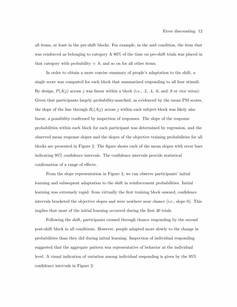
Error discounting 12

all items, at least in the pre-shift blocks. For example, in the mid condition, the item that

was reinforced as belonging to category A 80% of the time on pre-shift trials was placed in

that category with probability ' .8, and so on for all other items.

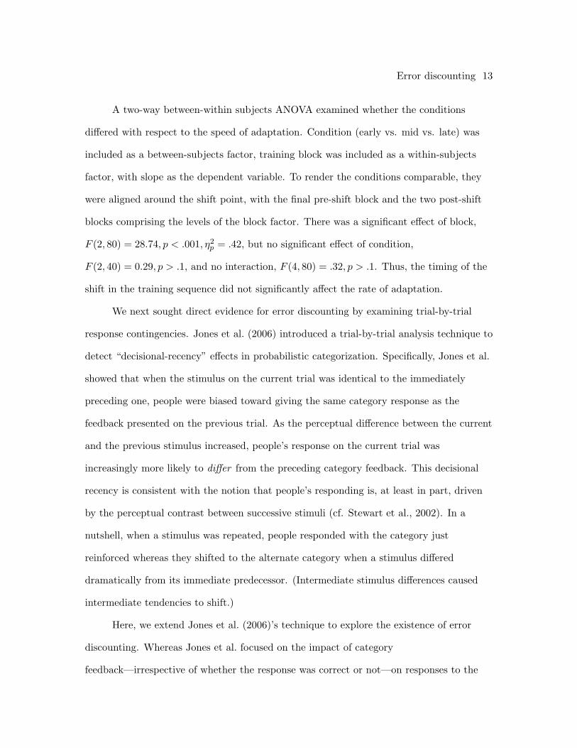
In order to obtain a more concise summary of people’s adaptation to the shift, a

single score was computed for each block that summarized responding to all four stimuli.

By design, P (A|j) across j was linear within a block (i.e., .2, .4, .6, and .8 or vice versa):

Given that participants largely probability-matched, as evidenced by the mean PM scores,

the slope of the line through Ri(A|j) across j within each subject-block was likely also

linear, a possibility confirmed by inspection of responses. The slope of the response

probabilities within each block for each participant was determined by regression, and the

observed mean response slopes and the slopes of the objective training probabilities for all

blocks are presented in Figure 2. The figure shows each of the mean slopes with error bars

indicating 95% confidence intervals. The confidence intervals provide statistical

confirmation of a range of effects.

From the slope representation in Figure 2, we can observe participants’ initial

learning and subsequent adaptation to the shift in reinforcement probabilities. Initial

learning was extremely rapid: from virtually the first training block onward, confidence

intervals bracketed the objective slopes and were nowhere near chance (i.e., slope 0). This

implies that most of the initial learning occurred during the first 40 trials.

Following the shift, participants crossed through chance responding by the second

post-shift block in all conditions. However, people adapted more slowly to the change in

probabilities than they did during initial learning. Inspection of individual responding

suggested that the aggregate pattern was representative of behavior at the individual

level. A visual indication of variation among individual responding is given by the 95%

confidence intervals in Figure 2.

Error discounting 13

A two-way between-within subjects ANOVA examined whether the conditions

differed with respect to the speed of adaptation. Condition (early vs. mid vs. late) was

included as a between-subjects factor, training block was included as a within-subjects

factor, with slope as the dependent variable. To render the conditions comparable, they

were aligned around the shift point, with the final pre-shift block and the two post-shift

blocks comprising the levels of the block factor. There was a significant effect of block,

F (2, 80) = 28.74, p < .001, η2p = .42, but no significant effect of condition,

F (2, 40) = 0.29, p > .1, and no interaction, F (4, 80) = .32, p > .1. Thus, the timing of the

shift in the training sequence did not significantly affect the rate of adaptation.

We next sought direct evidence for error discounting by examining trial-by-trial

response contingencies. Jones et al. (2006) introduced a trial-by-trial analysis technique to

detect “decisional-recency” effects in probabilistic categorization. Specifically, Jones et al.

showed that when the stimulus on the current trial was identical to the immediately

preceding one, people were biased toward giving the same category response as the

feedback presented on the previous trial. As the perceptual difference between the current

and the previous stimulus increased, people’s response on the current trial was

increasingly more likely to differ from the preceding category feedback. This decisional

recency is consistent with the notion that people’s responding is, at least in part, driven

by the perceptual contrast between successive stimuli (cf. Stewart et al., 2002). In a

nutshell, when a stimulus was repeated, people responded with the category just

reinforced whereas they shifted to the alternate category when a stimulus differed

dramatically from its immediate predecessor. (Intermediate stimulus differences caused

intermediate tendencies to shift.)

Here, we extend Jones et al. (2006)’s technique to explore the existence of error

discounting. Whereas Jones et al. focused on the impact of category

feedback—irrespective of whether the response was correct or not—on responses to the

Error discounting 14

following stimulus, we examined whether people’s response on trial n was affected by

whether or not their response on trial n− 1 was correct. That is, whereas Jones et al.

considered only the nature of the feedback on trial n− 1, we additionally determined

whether or not the probabilistic feedback n− 1 was identical to the response n− 1.

If people’s responding is subject to decisional recency, then the following

contingencies should be observed. If the same stimulus is repeated on two successive

trials, people should repeat their response if it was correct on the first trial but they

should shift to the alternate response following an error. Conversely, if the stimuli on two

successive trials are maximally different, then an error should be followed by the same

response whereas a correct response should be followed by a shift. (Intermediate stimulus

differences should again give rise to intermediate response tendencies.) If people gradually

come to discount errors, then those response contingencies should decrease across training

at least up to the shift in reinforcement probabilities. After the shift, those response

contingencies might re-emerge, albeit perhaps slowly.

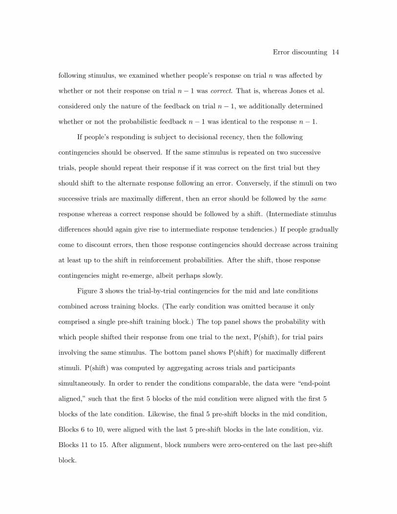
Figure 3 shows the trial-by-trial contingencies for the mid and late conditions

combined across training blocks. (The early condition was omitted because it only

comprised a single pre-shift training block.) The top panel shows the probability with

which people shifted their response from one trial to the next, P(shift), for trial pairs

involving the same stimulus. The bottom panel shows P(shift) for maximally different

stimuli. P(shift) was computed by aggregating across trials and participants

simultaneously. In order to render the conditions comparable, the data were “end-point

aligned,” such that the first 5 blocks of the mid condition were aligned with the first 5

blocks of the late condition. Likewise, the final 5 pre-shift blocks in the mid condition,

Blocks 6 to 10, were aligned with the last 5 pre-shift blocks in the late condition, viz.

Blocks 11 to 15. After alignment, block numbers were zero-centered on the last pre-shift

block.

Error discounting 15

The figure permits several conclusions: First, there is clear evidence for decisional

recency because for an identical stimulus (top panel), people tend to shift to the alternate

category following an error but they repeat the same category after a correct response.

Those response tendencies are reversed for the maximally different stimuli (bottom panel).

Second, there is evidence for error discounting because during the pre-shift blocks, P(shift)

gradually decreases following an error when the items are the same, and increases for

items that are different. That gradual process is reversed once reinforcement probabilities

are experimentally shifted and people become more sensitive to errors. We provide

statistical confirmation of this pattern in a joint analysis of both experiments once all data

have been presented.

Experiment 2

In Experiment 1, we focused on the consequences of sudden shifts in the

probabilistic environment. The purpose of Experiment 2 was to explore how people

respond to more gradual changes in the probabilistic structure. The consequences of error

discounting may be more pronounced and more prolonged when the probabilistic

environment shifts more gradually.

Method

Participants. The participants were 38 members of the University of Western

Australia community. Participants were randomly assigned to the two conditions, early

(n = 18) and late (n = 20). Of these participants, 9 were presented with square stimuli,

and 29 were presented with the circle and radial line stimuli. Participants received either

course credit or A$10 remuneration.

Stimuli and apparatus. The stimuli and apparatus were almost identical to that in

Experiment 1, with the following exceptions. As in Experiment 1, the feedback was given

Error discounting 16

on a probabilistic basis. Initially, the probability of an item belonging to category A was

.2, .4, .6, and .8, respectively, in increasing order of square size or radial line position.

Category B probabilities were 1− P (A). In the early condition, the probabilities shifted

from their starting values at the beginning of Block 7, viz. to .35, .45, .55, and .65,

respectively, for the four items. At the beginning of Block 9, the probabilities shifted

through chance to .65, .55, .45, and .35, before finally settling at .8, .6, .4, and .2 from the

beginning of Block 11. The probability of an item being in category B was always equal to

1− P (A). In the late condition, the probabilities shifted under the same schedule, except

that the shift occurred later in the sequence, beginning with Block 11 and finishing with

Block 15. The procedure was identical to Experiment 1.

Results and Discussion

PM scores were calculated over Blocks 5 and 6 for the Early condition, and 9 and 10

for the Late condition. Two and five participants were excluded from the early and late

conditions respectively, as their PM scores were below chance. As in Experiment 1, trials

with an RT of less than 150 ms or an RT of more than 4 SD above a participant’s mean

RT were removed from further analysis. Participants were removed if more than 10% of

their responses exceeded the RT criterions. Based on this criterion, an additional four

participants were removed from the early condition, and five from the late condition. The

mean PM scores for the remaining participants in the early and late conditions were 0.64

(SD = 0.27) and 0.65 (SD = 0.22). The mean scores for the early (t(11) = 8.18, p < .001)

and late (t(9) = 9.33, p < .001) conditions were significantly greater than chance. One

additional participant was removed from the late condition for the slope plots and for the

stimulus check. After removing trials with extreme reactions times, this participant had

no responses for two items in the final block, thus response slopes and PM scores could

Error discounting 17

not be calculated for the final block. This participant was retained for all other analyses

(unless otherwise specified).

As in Experiment 1, PM scores were next calculated for each of the 18 blocks. A

three-way between-within ANOVA (Condition × Stimulus type × Block) was run with

these PM scores as the dependent variable. The ANOVA uncovered no significant main

effect of stimulus type, F (1, 17) = 0.20, p > .1. Data were collapsed across stimulus type

for the remaining analysis.

Response slopes were computed in the same manner as for Experiment 1, and are

shown in Figure 4. In both conditions, participants adapted to the shift. There was,

however, notably little change in responding after the first partial shift in training

probabilities (i.e., in Blocks 7 and 8 in the early condition and in Blocks 11 and 12 in the

late condition). Participants appeared to adapt more to the second shift, with mean

slopes crossing through chance responding by Blocks 12 and 15 for the early and late

conditions respectively.

Participants appeared to learn more slowly after the shift than they did during

initial learning. The contrast in learning speeds between the pre- and post-shift learning

was more evident than in Experiment 1. In both conditions, pre-shift response slopes were

above the objective response slopes by Block 1. However, after the shift, the mean

response slopes do reach the objective training probabilities in either conditions.

A two-way between-within subjects ANOVA was conducted on the slope estimates.

The between-subjects factor was condition (early vs. late). The within-subjects factor was

blocks. Due to the gradual-shift design of the present experiment, the training-block

factor had 8 levels: these ranged from the two final pre-shift blocks to the second block

following the final shift. Thus, for the early condition, the 8 blocks were Blocks 4 to 12,

and for the late condition, they were Blocks 8 to 16. A Huynh-Feldt correction was used

to correct for violations of sphericity. The change in slope across blocks was significant,

Error discounting 18

F (3.72, 74.39) = 23.35, p < .001, η2p = .54, but there was no significant effect of condition,

F (1, 20) = 0.57, p > .1, and no interaction, F (3.72, 74.39) = 0.75, p > .1.

A decisional-recency analysis was conducted as in Experiment 1. The results of this

analysis are shown in Figure 5, with the upper and lower panels showing the P(shift) for

identical and maximally different pairs of stimuli, respectively. As for the first study, data

were simultaneously aligned on the first block and the block at which the training

probabilities shifted; that is, Block 6 for the early condition and Block 10 for the late

condition. As in Experiment 1, the P(shift) can be seen to decrease for identical items and

increase for the maximally dissimilar items with training.

Statistical confirmation of the apparent error discounting revealed by the

decisional-recency analysis in both Experiments 1 and 2 was provided by a multilevel

generalized linear model (Baayen, Davidson, & Bates, 2007). To maximize power of the

analysis, the mid and late conditions of Experiment 1 were analyzed together with the

mid and late condition from Experiment 2. The early condition of Experiment 1 was

excluded from the analysis as it had only one pre-shift block. Because the

decisional-recency analysis pointed to the gradual discounting of errors before

reinforcement probabilities were shifted, only pre-shift blocks were considered for each of

the conditions. Thus, from Experiment 1, the analysis included Blocks 1 to 10 and 1 to 15

for the mid and late conditions respectively. From Experiment 2, the analysis included

Blocks 1 to 6 and 1 to 10 for the early and late conditions respectively. To minimize the

influence of the less diagnostic trial-pair transitions involving moderately dissimilar pairs

of stimuli, only perceptual differences 0 (identity) and 3 (maximally dissimilar) were

considered. The dependent variable was whether or not the response on the current trial

differed from the preceding response (coded as 1 or 0). The perceptual difference between

the two consecutive stimuli (0 or 3) was entered as a fixed-effect factor and was fully

Error discounting 19

crossed with block and with a factor called ‘error-before’ which captured whether or not

an error had been made on the previous trial.

The results are summarized in Table 1 and confirm the pattern in Figures 3 and 5.

We highlight four effects: (a) The greater the perceptual difference between two successive

stimuli, the more likely people were to switch their response category. (b) An error was

more likely to be followed by a switch than a correct response. (c) Those two variables

interacted such that a switch became less likely with increasing perceptual difference if an

error had just been committed (compare the two panels of Figure 3 for a particularly clear

illustration of this interaction). (d) Crucially, the role of an error declined with blocks (EB

× block interaction), thus attesting to the presence of error discounting.

In summary, the trial-by-trial contingency data from both experiments replicated

the decisional recency previously reported by Jones et al. (2006). We additionally

established the presence of error discounting: People gradually adjusted the probability

with which they shifted their response on trials following errors.

Computational Modeling

Both experiments provided multiple indications for the presence of error discounting.

First, there was evidence for slower post-shift learning than during the initial learning; this

was particularly evident in Experiment 2. Second, in Experiment 2, there was a notable

delay in adaptation to the new reinforcement probabilities. Third, the decisional-recency

analysis showed that at a trial-by-trial level, people gradually came to ignore errors as

training progressed, even before reinforcement probabilities were shifted. We next turn to

quantitative modeling to investigate further the existence of error discounting. The aim of

using quantitative modeling was twofold. First, to verify whether an error-discounting

mechanism could improve the ability of computational models to account for the data.

Second, to pursue a theoretical exploration of the processes underlying error discounting.

Error discounting 20

We applied four models to the data. One model, the GCM (Nosofsky, 1986), was

used to explore a potential alternative explanation for error discounting based on sample

size. The other three models were the MAC model (Stewart et al., 2002), RASHNL

(Kruschke & Johansen, 1999), and ATRIUM (Erickson & Kruschke, 1998). In each of the

latter three models we instantiated a computational error-discounting mechanism. The

aim of including an error-discounting mechanism was to determine whether, after

controlling for the number of parameters, theories of categorization with an

error-discounting mechanism were able to better account for the data than theories

without error discounting. We give a brief summary of each model and the modeling

results below. Full details of the models, model fitting procedures, and model performance

can be found in the Appendix.

GCM. The GCM is an exemplar-based model that stores representations of all

previously encountered stimuli. The model categorizes new stimuli by making a similarity

comparison between the new stimulus and all stored exemplar representations. The GCM

was used to explore an alternative explanation for error discounting based on sample size.

It is possible that shifts in the feedback probabilities might have a small impact on

behavior simply due to the large number of stored exemplars consistent with the initial

training probabilities which “drown out” the later (and fewer) exemplars stored with the

revised training probabilities. Due to its exemplar-based architecture, the GCM was a

fitting choice to explore this sample-size explanation. The GCM contains two free

parameters. The first is a specificity parameter, c. The specificity parameter controls the

rate at which the psychological similarity to a stored exemplar decreases with increasing

perceptual distance from a given stimulus. The second parameter is a scaling parameter,

γ, that controls the decisional criterion of the model. The γ parameter can control

whether the model responds at chance, probability matches, or maximizes.

Error discounting 21

MAC. Unlike most of its rivals, the MAC model uses only feedback and perceptual

information from the previous trial (or limited set of trials) to make a category decisions.

If the previous item was categorized correctly, then the MAC is more likely to give the

same response to a perceptually similar item on the following trial. Conversely, the model

is more likely to give an alternative response to a perceptually different item. This

utilization of information from the immediately preceding trial(s) only makes the MAC

model a prime candidate for exploring the impact of error discounting at the level of

trial-by-trial decisional recency. Here we use the original MAC (Stewart et al., 2002), as

opposed to an extended version of the model (Stewart & Brown, 2004). As noted by

Stewart and Brown (2004), with greater trial memory, the MAC approaches the behavior

of the GCM. Thus, the original MAC (with a single-trial memory) can provide greater

comparative contrast to the GCM than can the extended MAC.

The MAC has a single parameter, b, which controls the rate at which the

psychological similarity to the previous stimuli decreases with greater perceptual

similarity between the current and previous items. We instantiated an error-discounting

mechanism in the MAC by gradually attenuating the role of the previous stimulus for

trials following an error. Specifically, we used two separate values of b following correct

and following incorrect responses, respectively, and the value of b following incorrect

responses was reduced by a factor r on each trial, given by:

r = 1/(1 + ρ), (2)

where ρ was a free parameter that controlled the rate at which the similarity parameter, b,

was reduced.

RASHNL. RASHNL is an exemplar-based model of associative learning. The model

is an extension of the exemplar model ALCOVE (Kruschke, 1992). Like the GCM,

Error discounting 22

RASHNL makes categorization decisions on the basis of a similarity comparison between

the present stimulus and all stored exemplar stimuli. Unlike the GCM, RASHNL includes

an error-based, associative-learning mechanism that controls the strength of association

weights between exemplars and categories. The standard version of RASHNL can also

learn to distribute its attention across stimulus dimensions. Due to the use of a

single-dimension task, the attention features of RASHNL were not required for the present

simulations.

RASHNL was chosen for its built-in error-discounting mechanism. The mechanism

in RASHNL works by decreasing, or “annealing,” the rate at which the model learns the

associations between exemplars and categories. On each trial, an association learning rate,

λ, is multiplied by the factor r, given in (2). As before, ρ is a free parameter controlling

the rate at which the learning rate is reduced across trials. Higher value of ρ lead to fast

annealing. As RASHNL uses errors to learn, by annealing the learning rates, as training

progresses, RASHNL effectively ignores errors. RASHNL has two additional parameters,

c, and ϕ, that are equivalent to the GCM’s specificity parameter, c, and the decision

criterion parameter, γ, as outlined above.

rATRIUM. To extend the potential generality of our conclusions beyond exemplar-

and recency-based models, we also included a rule-based variant of ATRIUM (Erickson &

Kruschke, 1998). At present both rule and exemplar models are popular within the

probabilistic categorization literature, with prior research providing conflicting support for

each type of model (Juslin, Jones, Olsson, & Winman, 2003; Kalish & Kruschke, 1997;

McKinley & Nosofsky, 1995; Rouder & Ratcliff, 2004). As the present study is not

designed to distinguish between these models types, we included a rule-based model to

ensure that any results were not specific to a particular type of theory. The full version of

ATRIUM is a hybrid rule and exemplar model. For present purposes we used only the

rule module, which we term, rATRIUM. rATRIUM categorizes items by dividing the

Error discounting 23

category space by a rule boundary. Each side of this boundary is associated with a

particular category. The further a new item falls on one side of the boundary, the more

likely it is that the item will be placed in the associated category. Like RASHNL,

rATRIUM has an associative-learning mechanism. This associative learning mechanism

allows rATRIUM to learn associations between categories and each side of the category

boundary. To explore error discounting, we implemented the same error-discounting

mechanism in rATRIUM as in RASHNL. As in RASHNL, rATRIUM’s learning-rate

parameter, λ, was annealed across training. The parameter, λ, controls the rate at which

rATRIUM learns associations between categories and each side of the category boundary.

The annealing rate was controlled by the free parameter ρ, as given in (2). rATRIUM

includes two additional free parameters, a noise parameter, µ, which controls the standard

deviation of perceptual noise around the rule boundary. Greater values of µ, decrease the

ability of the model to distinguish an item’s location relative to the rule boundary. The

final parameter, ϕ, is a decision criterion parameter, equivalent to the γ and ϕ parameters

in the GCM and RASHNL, respectively.

Model Fitting Procedures and Modeling Results

For the three models with an error-discounting mechanism, the MAC, RASHNL,

and rATRIUM, we ran two sets of fits, one with the error-discounting mechanism

functioning, and one with it switched off. The models were fit at the level of individuals

by maximizing the binomial log-likelihood.

Table 2 summarizes the fit statistics (i.e., negative log-likelihoods, Akaike

information criterion, AICc, and Bayesian information criterion, BIC) for each of the

models (figures of the model predictions can be found in the Appendix). From the table,

the GCM provided a poor account of the results, with relatively high AICc and BIC

values than compared to RASHNL and rATRIUM. From inspection of the model

Error discounting 24

predictions, the GCM was unable to adapt to the shift as fast as participants did in all

conditions, with the exception of the early condition of Experiment 1. The poor

performance of GCM rules out the sample-size explanation of error discounting.

RASHNL, with annealing on, provided the best account of the data. Inspection of

the model predictions showed that RASHNL provided a good quantitative fit of the data,

closely capturing the participant’s behavior throughout the shift in all conditions. The fits

of RASHNL with annealing on were followed by rATRIUM with annealing on, and then

RASHNL and rATRIUM with annealing off. The MAC did not provide a good

quantitative fit; however, inspection of the best-fitting predictions of the model showed

that the MAC qualitatively captured the data, including the shift in reinforcement.

Crucially, for all three models with an error-discounting mechanism, the fits were

better when the mechanism was turned on than when it was off. For the MAC, RASHNL,

and rATRIUM, lower AICc and BIC values were obtained when annealing was on than

when annealing was off. Likelihood-ratio tests confirmed that each of the models fit

significantly better when they included an annealing mechanism (RASHNL:

χ2(65) = 1034.81, p < .001, rATRIUM: χ2(65) = 1313.56, p < .001, MAC:

χ2(64) = 2547.14, p < .001). The fact that all three models fit better with error

discounting suggests that (a) error discounting is required to accurately capture

probabilistic categorization behavior, and (b) that this holds true regardless of the

particular type of category representation.

General Discussion

Summary of Findings

The present article sought to investigate (a) whether people gradually tend to

discount errors during probabilistic categorization, and (b) what the underlying

mechanism of error discounting are, if present. Taken together, the results clearly reveal

Error discounting 25

the presence of error discounting during probabilistic category learning. Error discounting

can be inferred from (a) the difference between the initial fast learning and the slower

post-shift learning, (b) the apparent lack of adaptation to the first partial shift in

Experiment 2, (c) the decline in likelihood with which participants shifted their category

response on trials following an error, and (d) the fact that both associative-learning

models and the MAC model handled the data significantly better when they included an

error-discounting mechanism than when they did not.

The present evidence for error discounting is generally consistent with previous

findings (Edgell, 1983; Edgell & Morrissey, 1987) that implicated the presence of

annealing in models of categorization (Kruschke & Johansen, 1999). Unlike those

precedents, however, the unidimensional design of the present studies precluded

alternative interpretations based on blocking. Before we discuss the implications of our

results, we briefly address some possible limitations.

Limitations and Concerns

Participants in our studies were not informed about a possible change in the

probabilistic environment. In the natural world, by contrast, people may be more wary of

changing probabilities and might thus adapt faster than observed here. However, the fact

that learning in Experiment 2 continued to be slow after participants had transited

through chance responding—at which point they would likely be aware of the changed

reinforcement probabilities—suggests that awareness of a shift might not prevent (or

undo) error discounting. Moreover, the decisional-recency analysis that showed a decline

in the probability of shifting responses following errors, was run on pre-shift blocks only.

Thus, people were shown to discount errors even before any shift had taken place. The

shift in reinforcement probabilities thus helped highlight the existence of error

discounting; however, it was not critical for error discounting to occur and to be detected.

Error discounting 26

Critics might also puzzle why the extent of pre-shift training failed to have any

effect. If error discounting is gradual, why did people’s adaptation rate not decrease with

more pre-shift training? Our response is twofold: First, given the relative simplicity of our

task, even limited training may have been sufficient to induce at least some discounting.

This possibility is supported by the finding that even after the very first block of training,

performance was far above chance and probability matching close to the objective target.

It is also supported by the visible trends in the decisional-recency analysis. Second,

RASHNL and rATRIUM required annealing for their account of the data, irrespective of

the extent of pre-shift training and even when parameter values were constrained to be

identical across conditions. This finding confirms that error discounting commenced early

on during training and then continued throughout the experiment.

Turning to potential theoretical limitations, we note that the use of a single stimulus

dimension—while eliminating an alternative blocking explanation—rendered the attention

and gain features of RASHNL and rATRIUM irrelevant. As it is assumed in RASHNL

that the attention and gain learning rates are also annealed (Kruschke & Johansen, 1999),

the role of these features must therefore await further exploration. Likewise, it remains

unclear how discounting operates in multi-dimensional environments. On the one hand,

error discounting may play a greater role in complex environments, because if people have

more difficulty determining the underlying probability structure, they may show a greater

tendency to ignore errors. On the other hand, it may be that with multi-dimensional

stimuli, error discounting is overshadowed by blocking effects, and thus has little impact

on its own.

Finally, error discounting might interact with other effects and strategies present in

multi-dimensional probabilistic categorization. For instance, Little and Lewandowsky

(2009a) showed that compared to a deterministic condition, participants learning an

identical category structure under probabilistic reinforcement spread their attention across

Error discounting 27

a wider selection of possible cues. Specifically, people detected a non-diagnostic

correlation among cues that escaped notice under deterministic learning conditions. It

follows that in multi-dimensional categorization, error discounting might only have an

impact once alternative strategies (i.e., attentional allocations) have been exhausted.

Those issues await resolution by future research.

Theoretical Implications

In the present study we used three types of categorization models; an exemplar

model, a rule-based model, and a recency-based model, to explore the existence of error

discounting. The present study was not designed to distinguish between these types of

categorization models, nor was it designed to determine how people represent categories.

Instead, the inclusion of the three model types demonstrated that regardless of how

categories are represented, error discounting is important to account for probabilistic

categorization behavior. We therefore conclude that annealing of learning rates and error

discounting deserve a prominent theoretical role in approaches to probabilistic

categorization.

If we accept the necessity for error discounting, how is it best described at a

conceptual level? Does error discounting reflect an on-going and ever-increasing

habituation to a constant error signal? Alternatively, does error discounting reach a

plateau, thus effectively differentiating between two error signals—one that is unavoidable

due to the probabilistic environment and (potentially) another one that is unexpected and

arises from changes in the environment?

The former alternative corresponds to the instantiation of annealing in RASHNL

and rATRIUM, whose learning rates ultimately and inevitably reach 0 (whereupon no

further adaptation to a shift occurs, as confirmed by simulations involving a large amount

of additional pre-shift training that are not reported in detail here). If people, as assumed

Error discounting 28

by the models, progressively discount more and more error, how would they notice a

gradual shift in reinforcement probabilities (as in our Experiment 2), and how would they

learn from it? One possibility is that not all feedback-based learning is error driven.

Indeed, there is recent neuroscientific (Histed, Pasupathy, & Miller, 2009) and behavioral

(Smith & Kimball, 2010) evidence that people are capable of learning from feedback on

correct responses. These recent findings run contrary to the common error-focused

assumptions of connectionist models (e.g., Gluck & Bower, 1988a, 1988b; Rumelhart et

al., 1986). We are not aware of any connectionist learning that is driven by correct

responses, although these recent results (Histed et al., 2009; Smith & Kimball, 2010) may

stimulate developments in that direction.

The latter alternative, namely that error-discounting reaches a plateau, is not

currently instantiated in RASHNL and rATRIUM but nonetheless seems rather attractive

for two reasons: First, people in both experiments were responsive to shifts, albeit

sometimes with a considerable delay (in Experiment 2). Second, the extent of pre-shift

training did not affect people’s responsiveness to the shift in either experiment. This

result is difficult to reconcile with a notion of growing habituation to error and it is more

compatible with the idea that a certain amount of error is discounted, but that any

further error is used for associative learning.

The idea that people discount some variability in the error signal resonates with the

idea that people adjust their strategies avoid over-fitting or, in other words,

overcompensating for noise (Myung & Pitt, 2004). The idea of over-fitting is germane if

we assume that participants are in effect trying to distinguish some true feedback signal

from variation or noise within that signal. Hence, participants might be aware that the

overall environment has changed but are unaware of the extent of that change. Error

discounting can therefore be viewed as a rational way to exclude excess variation from

influencing learning. This is similar to modern machine learning algorithms which

Error discounting 29

typically include a regularizing term (i.e., a penalty on the fitting measurement) to

effectively limit the types of patterns that can be learned and reduce over-fitting (Bishop,

2006). Other approaches, such as the Bayesian learning approach we consider below (see

e.g., Bishop, 2006, Chapter 3), implement regularization through use of prior probability

distributions over relevant patterns.

The observation that error discounting exists at the level of decisional-recency flags

the importance of considering corrective feedback when exploring sequential effects in

categorization. Previous analyzes of decisional-recency effects (e.g., Jones et al., 2006;

Stewart et al., 2002) have focused on the impact of category-label feedback irrespective of

whether or not the previous response was an error. As we have observed, people react

differently following errors and correct responses; additionally, people adjust their behavior

in response to errors over time. These reactions to errors in categorization suggest that it

is important to consider corrective feedback when exploring decisional-recency effects.

So far, the focus here has been on participants’ tendency to ignore error-based

corrective feedback information. While participants did tend to discount errors, and thus

ignored feedback, participants simultaneously showed signs of precise utilization of

feedback information, as evidenced by people’s highly-accurate probability-matching

behavior. In the present tasks, the probability with which people categorized items

approximated the probability with which the items belonged to each category. This

accurate probability matching cannot arise without accurately observing the feedback

information. Thus, participants simultaneously exhibited precise utilization of feedback

information and a tendency to ignore feedback information. This duality of the utilization

of feedback information is counter-intuitive: How can people dismiss feedback while being

demonstrably attuned to it at the same time? The answer is implied by our modeling:

The probability-matching behavior is established early on, when associations between

stimuli and outcomes are learned on the basis of feedback. Once established, those

Error discounting 30

associations persist (unless a reversal shift takes place) despite the increasing discounting

of errors and the associated feedback.

Links to Bayesian Perspectives on Category Learning

The recent popularity of probabilistic-descriptive approaches to cognition (e.g.,

Chater, Tenenbaum, & Yuille, 2006) raises the possibility that error discounting might be

tractable within a Bayesian approach. Bayesian approaches to cognition take into account

our beliefs and expectations in the form of a prior probability distribution over potential

hypotheses. Our prior beliefs are transformed into posterior beliefs in light of new data;

hypotheses which are consistent with the data are maintained whereas inconsistent

hypotheses are discarded. In our task, as knowledge accumulates about the probability

with which each item falls into each category, the distribution that represents those beliefs

becomes more peaked and less variable with continued training. Hence, the influence of

each individual stimulus on the posterior expectations of an item’s category membership

decreases: Less variable prior distributions require more new evidence (i.e., higher error

rates) in order for new hypotheses to have any weight in the posterior. Error discounting

may thus be interpretable in Bayesian terms as reflecting the continued “sharpening” of

the distribution over the reinforcement rate of each item.

Implications of Error Discounting

Although our work was confined to probabilistic categorization, we can draw some

connections to other situations involving decision making and industrial processes.

One perspective on error-discounting is that people minimize cognitive

“expenditure” by dismissing the feedback signal that would otherwise entail further

learning. This reduction in cognitive expenditure is also at the heart of the simple

heuristics that underlie much of human decision making, and which have been

characterized as maximizing our return on the investment of cognitive effort (Gigerenzer,

Error discounting 31

Todd, & ABC Research Group, 1999). Similar to decision making heuristics—such as the

recognition heuristic (Goldstein & Gigerenzer, 1999, 2002)—error discounting is highly

adaptive for environments with unavoidable error, in which continuing to attend to errors

entails no benefit for accuracy, whereas ignoring errors may free up limited cognitive

resources.

However, in the same way that decision-making heuristics may incur a cost when

the environment fails to conform to people’s expectations (Tversky & Kahneman, 1974),

error discounting can also incur a high cost in some environments. For example, pilots

who ignore frequent warnings from an autopilot system are at increased risk of causing an

accident (Farrell & Lewandowsky, 2000; Parasuraman & Riley, 1997; see also,

Moray2007). High false alarm rates for automated error detection systems result in people

slowing their response to, or simply ignoring warnings about potential errors

(Parasuraman & Riley, 1997). For example, in a task monitoring the navigation, speed,

power and cargo systems of a ship, if the system sets off frequent false error alarms,

participants eventually ignore these warnings signals (Kerstholt & Passenier, 2000). With

frequent false alarms, participants made fewer attempts to gain information needed to

asses the problem, and were slower to access this information when they did. This

behavior constitutes a good analog to the error discounting observed in our studies.

However, in many real-life situations, poor reliability of automated systems interacts with

the complexity of those systems, thus arguably engendering error discounting in precisely

those situations in which it is least advisable. Future work on trust in automation

(Lewandowsky, Mundy, & Tan, 2000) is necessary to delineate the circumstances in which

such inadvisable error discounting may occur.

Error discounting 32

References

Akaike, H. (1974). A new look at the statistical model identification. IEEE Transactions

on Automatic Control , 19 , 716–723.

Amari, S. (1967). Theory of adaptive pattern classifiers. IEEE Transcriptions in

Electronic Computers, 16 , 299–307.

Ashby, F. G., & Maddox, W. T. (1993). Relations between prototype, exemplar, and

decision bound models of categorization. Journal of Mathematical Psychology , 37 ,

372–400.

Baayen, R. H., Davidson, D. J., & Bates, D. M. (2007). Mixed-effects mode with crossed

random effects for subjets and items. Journal of Memory and Language, 59 ,

390–412.

Bishop, C. M. (2006). Pattern recognition and machine learning. Cambridge: Springer.

Blair, M., & Homa, D. L. (2005). Integrating novel dimensions to eliminate category

exceptions: When more is less. Journal of Experimental Psychology: Learning,

Memory, & Cognition, 31 , 258–271.

Bos, S., & Amari, S. (1998). On-line learning in switching and drifting environments with

application to blind sources separation. In D. Saad (Ed.), On-line learning in neural

networks (pp. 209–230). Cambridge: Cambridge University Press.

Brainard, D. H. (1997). The psychophysics toolbox. Spatial Vision, 10 , 433–436.

Chater, N., Tenenbaum, J. B., & Yuille, A. (2006). Probabilistic models of cognition:

Conceptual foundations. Trends in Cognitive Science, 10 , 287–291.

Colreavy, E., & Lewandowsky, S. (2008). Strategy development and learning differences in

supervised and unsupervised categorization. Memory & Cognition, 36 , 762–775.

Darken, C., & Moody, J. E. (1991). Note on learning rate schedules for stochastic

optimization. In R. P. Lippman, J. E. Moody, & D. S. Tourestzky (Eds.), Advances

in neural information processing systems (pp. 832–838). San Mateo, CA: Kaufmann.

Error discounting 33

Edgell, S. E. (1983). Delayed exposure to configural information in nonmetric

multiple-cue probability learning. Organizational Behavior and Human Decision

Processes, 32 , 55–65.

Edgell, S. E., & Morrissey, J. M. (1987). Delayed exposure to additional relevant

information in nonmetric multiple-cue probability learning. Organizational Behavior

and Human Decision Processes, 40 , 22–38.

Erickson, M. A., & Kruschke, J. K. (1998). Rules and exemplars in category learning.

Journal of Experimental Psychology: General , 127 , 107–140.

Erickson, M. A., & Kruschke, J. K. (2002). Rule-based extrapolation in perceptual

categorization. Psychonomic Bulletin & Review , 9 , 160–168.

Estes, W. K. (1984). Global and local control of choice behavior by cyclically varying

outcome probabilities. Journal of Experimental Psychology: Learning, Memory, &

Cognition, 10 , 258–270.

Estes, W. K., & Straughn, J. H. (1954). Analysis of a verbal conitioning situation in terms

of statistical learning theory. Journal of Experimental Psychology , 47 , 225–234.

Fantino, E., & Esfandiari, A. (2002). Probability matching: encouraging optimal

responding in humans. Canadian Journal of Experimental Psychology , 56 , 58–63.

Farrell, S., & Lewandowsky, S. (2000). A connectionist model of complacency and

adaptive recovery under automation. Journal of Experimental Psychology: Learning,

Memory, & Cognition, 26 , 395–410.

Friedman, D., & Massaro, D. W. (1998). Understanding variability in binary and

continuous choice. Psychonomic Bulletin & Review , 5 , 370–389.

Friedman, M. P., Burke, C. J., Cole, M., Kellyer, L., Millward, R. B., & Estes, W. K.

(1964). Two-choice behaviour under extended training with shifting probabilities. In

R. C. Atkinson (Ed.), Studies in mathematical psychology (pp. 250–316). California:

Error discounting 34

Stanford University Press.

Gigerenzer, G., Todd, P. M., & ABC Research Group the. (1999). Simple heuristics that

make us smart. New York: Oxford University Press.

Gluck, M. A., & Bower, G. H. (1988a). Evaluating an adaptive network model of human

learning. Journal of Memory and Language, 27 , 166–195.

Gluck, M. A., & Bower, G. H. (1988b). From conditioning to category learning: An

adaptive network model. Journal of Experimental Psychology: General , 117 ,

227–24.

Goldstein, D. G., & Gigerenzer, G. (1999). The recognition heuristic: how ignorance

makes us smart. In G. Gigerenzer, P. M. Todd, & the ABC Research Group (Eds.),

Simple heuristics that make us smart (pp. 37–58). New York: Oxford University

Press.

Goldstein, D. G., & Gigerenzer, G. (2002). Models of ecological rationality: the

recognition heuristic. Psychological Review , 109 , 75–90.

Heskes, T. M., & Kappen, B. (1991). Learning process in neural networks. Physical

Review A, 44 , 2718–2726.

Histed, M. H., Pasupathy, A., & Miller, E. K. (2009). Learning substrates in the primate

prefrontal cortex and striatum: sustained activity related to successful actions.

Neuron, 63 , 244–253.

Jones, M., Love, B. C., & Maddox, W. T. (2006). Recency effects in category learning.

Journal of Experimental Psychology: Learning, Memory, & Cognition, 32 , 316–332.

Juslin, P., Jones, S., Olsson, H., & Winman, A. (2003). Cue abstraction and exemplar

memory in categorization. Journal of Experimental Psychology: Learning, Memory,

and Cognition, 29 , 924–941.

Kalish, M. L., & Kruschke, J. K. (1997). Decision boundaries in one-dimensional

categorization. Journal of Experimental Psychology: Learning, Memory, and

Error discounting 35

Cognition, 23 , 1362–1377.

Kamin, L. J. (1969). Punishment. In B. A. Campbell & R. M. Church (Eds.), (pp.

279–296). New York: Appleton-Century-Crofts.

Kerstholt, J. H., & Passenier, P. O. (2000). Fault management in supervisory control: the

effect of false alarms and support. Ergonomics, 43 , 1371–1389.

Kruschke, J. K. (1992). ALCOVE: An exemplar-based connectionist model of category

learning. Psychological Review , 99 , 22–44.

Kruschke, J. K., & Blair, N. J. (2000). Blocking and backward blocking involve learned

inattention. Psychonomic Bulletin & Review , 7 , 636–645.

Kruschke, J. K., & Johansen, M. K. (1999). A model of probabilistic category learning.

Journal of Experimental Psychology: Learning, Memory, and Cognition, 25 ,

1083–1119.

Lamberts, K. (1997). Process models of categorization. In K. Lamberts & D. Shanks.

(Eds.), Knowledge, concepts, and categories (pp. 371–403). Hove, East Sussex:

Psychology Press.

Lewandowsky, S. (1995). Base-rate neglect in ALCOVE: A critical reevaluation.

Psychological Review , 102 , 185–191.

Lewandowsky, S., Mundy, M., & Tan, G. (2000). The dynamics of trust: Comparing

humans to automation. Journal of Experimental Psychology: Applied , 6 , 104–123.

Little, D. R., & Lewandowsky, S. (2009a). Better learning with more error: probabilistic

feedback increases sensitivity to correlated cues in categorization. Journal of

Experimental Psychology: Learning, Memory, & Cognition, 35 , 1041–1061.

Little, D. R., & Lewandowsky, S. (2009b). Beyond non-utilization: irrelevant cues can

gate learning in probabilitic categorization. Journal of Experimental Psychology:

Human Perception & Performance, 35 , 530–550.

Error discounting 36

Lorenz, B., & Parasuraman, R. (2007). Automated and interactive real-time systems. In

F. T. Durso, R. Nickerson, S. Dumais, S. Lewandowsky, & T. Perfect (Eds.),

Handbook of applied cognition (pp. 415–441). Chichester, England: Wiley.

Luce, R. D. (1963). Detection and recognition. In R. D. Luce, R. R. Bush, & E. Galanter

(Eds.), Handbook of mathematical psychology (pp. 103–189). New York: Wiley.

McKinley, S. C., & Nosofsky, R. M. (1995). Investigations of exemplar and decision bound

models in large, ill-defined category structures. Journal of Experimental Psychology:

Human Perception and Performance, 21 , 128–148.

Moray, N. (2007). Industrial systems. In F. T. Durso, R. Nickerson, S. Dumais,

S. Lewandowsky, & T. Perfect (Eds.), Handbook of applied cognition (pp. 281–305).

Chichester, England: Wiley.

Muller, K.-R., Ziehe, A., Murata, N., & Amari, S. (1998). On-line learning in switching

and drifting environments with application to blind source separation. In D. Saad

(Ed.), On-line learning in neural networks (pp. 93–110). Cambridge: Cambridge

University Press.

Murata, N., Kawanabe, M., Ziehe, A., Muller, K.-R., & Amari, S. (2002). On-line learning

in changing environments with applications to supervised and unsupervised learning.

Neural Networks, 15 , 743–760.

Myung, I.-J., & Pitt, M. A. (2004). Model comparison methods. Methods in Enzymology ,

383 , 351–366.

Nelder, J. A., & Mead, R. (1965). A simplex method for function minimization.

Computer Journal , 7 , 308–313.

Nosofsky, R. M. (1986). Attention, similarity and the identification-categorization

relationship. Journal of Experimental Psychology: General , 115 , 39–57.

Nosofsky, R. M., & Johansen, M. K. (2000). Exemplar-based accounts of

“multiple-system” phenomena in perceptual categorization. Psychonomic Bulletin &

Error discounting 37

Review , 7 , 375–402.

Parasuraman, R., & Riley, V. (1997). Humans and automation: use, misuse, disuse,

abuse. Human Factors, 39 , 230–253.

Pelli, D. G. (1991). The videotoolbox software for visual psychophysics: Transforming

numbers into movies. Spatial Vision, 10 , 437–442.

Rescorla, R. A., & Wagner, A. R. (1972). Classical conditioning: II. current research and

theory. In A. H. Black & W. F. Prokasky (Eds.), (pp. 64–99). New York:

Appleton-Century-Crofts.

Rouder, J. N., & Ratcliff, R. (2004). Comparing categorization models. Journal of

Experimental Psychology: General , 133 , 63–82.

Rumelhart, D. E., Hinton, G. B., & Williams, R. J. (1986). Learning internal

representations by back-propagation errors. In D. E. Rumelhart & J. L. McClelland

(Eds.), Parallel distributed processing: Explorations in the microstructure of

cognition (Vol. 1, pp. 318–362). Cambridge, MA: MIT Press.

Shanks, D. R., Tunney, R. J., & McCarthy, J. D. (2002). A re-examination of probability

matching and rational choice. Journal of Behavioral Decision Making , 15 , 233–250.

Smith, T. A., & Kimball, D. R. (2010). Learning from feedback: spacing and

delay-retention effects. Journal of Experimental Psychology: Learning, Memory, &

Cognition, 36 , 80–95.

Stewart, N., & Brown, G. D. A. (2004). Sequence effects in the categorization of tones

varying in frequency. Journal of Experimental Psychology: Learning, Memory, and

Cognition, 30 , 416-430.

Stewart, N., Brown, G. D. A., & Chater, N. (2002). Sequence effects in categorization of

simple perceptual stimuli. Journal of Experimental Psychology: Learning, Memory,

and Cognition, 28 , 3–11.

Error discounting 38

Tversky, A., & Kahneman, D. (1974). Judgment under uncertainty: Heuristics and biases.

Science, 185 , 1124–1131.

Wagenmakers, E.-J., & Farrell, S. (2004). AIC model selection using Akaike weights.

Psychonomic Bulletin & Review , 11 , 192–196.

Wickens, C. (2007). Aviation. In F. T. Durso, R. Nickerson, S. Dumais, S. Lewandowsky,

& T. Perfect (Eds.), Handbook of applied cognition (pp. 361–389). Chichester,

England: Wiley.

Yelen, D. R., & Yelen, D. (1969). The overt reversal effect in a probability learning

situation. Psychonomic Science, 14 , 152.

Error discounting 39

Appendix

Supplementary Material: Additional Computational Modeling Details

and Additional Results

Craig, Lewandowsky, and Little (submitted) explored the existence of error

discounting in probabilistic categorization. Part of their analysis involved the use a series

of computational models, the GCM (Nosofsky, 1986), MAC (Stewart et al., 2002),

RASHNL (Kruschke & Johansen, 1999), and ATRIUM (Erickson & Kruschke, 1998).

Craig et al. (submitted) found that the MAC, RASHNL, and ATRIUM fit data from two

probabilistic categorization experiments significantly better when they included a

mechanism to discount errors. The GCM did not include an error-discounting mechanism,

instead poor performance of GCM ruled out an alternative sample-size explanation for

error discounting. This supplement provides additional details of the models, modeling

procedures, and results from the fits with each of the four models.

GCM: A Sample-Size Explanation

A possible explanation for the experimental results in Craig et al. (submitted) was

that the slow post-shift learning was not due to a discounting of error, but instead was an

automatic by-product of the inevitable increase in memorized “sample size” during

learning. Specifically, in the very early stages of training, when few items had been

presented, on an exemplar view each further individual stimulus will have a relatively large

impact. However, at later stages of learning, new items become increasingly insignificant

in relation to the overall number of exemplars already encountered and memorized, thus

limiting their impact. The slow adaptation to the shift in the experiments could therefore

result from the small impact of items later in training relative to items early in training.

We explored this alternative within the GCM (Nosofsky, 1986). The GCM contains no

Error discounting 40

associative learning mechanism but represents all encountered instances in memory, thus

providing a quantitative instantiation of the sample-size hypothesis.

GCM Specification. The GCM assumes that on each trial the current item activates

all previously encountered stimuli stored in memory according to:

sij = exp(−c× dij), (A1)

where the similarity, sij , between items i and j is determined by the distance between

them in psychological space, dij = |xi − xj | , which in the present case involves only a

single dimension. (Note that for simplicity of exposition, all equations reported in this

supplement are tailored to the fact that our stimuli were uni-dimensional.) The specificity

parameter, c, determines the sharpness of the exponential function.

Similarities are converted to response probabilities by applying Luce’s choice rule

(Luce, 1963):

P (A|i) =(∑

j∈A sij)γ

(∑

j∈A sij)γ + (∑

j∈B sij)γ), (A2)

where the response scaling parameter, γ, allows responding to vary between

probability-matching when γ ' 1 and maximizing when γ � 1 (Ashby & Maddox, 1993;

Nosofsky & Johansen, 2000). Thus, upon presentation of a test stimulus, it is compared

against all stored exemplars in each of the categories separately, and a response is selected

based on which category yields the greatest summed similarity.

GCM Simulations. For the square stimuli used in the present study, the perceived

psychological distance between adjacent stimuli has been shown to be equivalent to the

actual perceptual distance between the stimuli (Colreavy & Lewandowsky, 2008). Thus,

for the simulations, the four stimuli were coded as the integers 1 to 4. The GCM was fit

separately to each participant’s mean response probabilities for all items in all blocks. The

Error discounting 41

GCM was presented with the training sequences shown to participants. Parameters (c and

γ) were capped at 25. Both parameters were estimated using the SIMPLEX algorithm

(Nelder & Mead, 1965) to minimize the negative binomial log-likelihood:

− lnL = −∑i

di ln(pi) + (ni − di) ln(1− pi), (A3)

where pi is the model’s predicted probability of category A for item i, di is the observed

number of A responses made for item i, and ni is the number of times item i was

presented.

Table A1 shows the GCM’s estimated parameters for both experiments. As shown

in Figures A1 and A2, the GCM failed to capture the data in some crucial ways: In

particular, it was unable to adjust its predictions in response to the probability shift. The

GCM only managed to capture the early condition of Experiment 1, presumably because

only 10 presentations of each item had occurred before the shift. However, in all other

conditions, the GCM could not accumulate enough new evidence within the number of

training trials to reverse its predicted probabilities. (Note, however, that there is a

downward trend in the predicted slopes after the shifts, which indicates that given

massively extended training, the GCM’s performance might come to mirror the final

outcome probabilities). In conclusion, the experimental results in Craig et al. (submitted)

cannot be accommodated by an explanation based solely on memorized sample size.

MAC model: Error discounting and Decisional Recency

The MAC model (Stewart et al., 2002) makes categorization decisions based only on

perceptual and feedback information provided on the previous trial. With the exception of

the immediately preceding item, the MAC model does not retain a representation of

previously encountered exemplars.

Error discounting 42

Formal description of the MAC model. We present two versions of the MAC model.

The first is the standard version of the model as outlined by Stewart et al. (2002). The

second is a new version of the model, modified to incorporate error discounting via an

annealing mechanism.

The MAC model makes categorization decisions by computing the psychological

distance between the current stimulus and the previous one (this distance is isomorphic to

the perceptual difference used in our decisional-recency analysis). The probability of

repeating the same category response, P(same), is given by:

P (same category) = e−bd2

(A4)

where d is the psychological distance between the current and previous stimulus, and b is

a constant controlling the steepness of the Gaussian generalization gradient. Thus, b

controls the rate at which psychological distance required to respond with a different

category than the previous trial. Lower values of b will result in stimuli being perceived as

more similar, thus increasing the probability that the response on the current trial will

match the category feedback given on the previous trial.

The second, modified version of the MAC model includes an error-discounting

mechanism, implemented by annealing the parameter b for trials following an error.

Specifically, b was set to decrease across trials in this version, thus forcing the model to

treat all items as if they were similar to the one just seen on the previous trial. Thus, the

model effectively ignores the feedback from trials following errors.

To incorporate the error-discounting mechanism, we generated two forms of

Equation A4. The first form of the equation was used on trials for which the response

given on the previous trial was correct. The second version of the equation was used on

trials following an error and instantiated annealing using the formalism provided in

Error discounting 43

RASHNL (Kruschke & Johansen, 1999). For this second form of the equation, the initial

value of b was multiplied by an annealing factor, r, given by:

r(t) = 1/(1 + ρ× t), (A5)

where ρ is a freely estimated, non-negative, scheduling parameter that controls the rate of

annealing. Larger values of ρ lead to faster annealing, and when ρ is clamped at zero, the

model exhibits no annealing at all (and saves a parameter in the process). This annealing

mechanism has the effect of reducing the steepness of the Gaussian generalization gradient

on the psychological distance between pairs of stimuli over trials. Thus, the mechanism

gradually reduces the probability with which the model will shift its category response on

a trial following an error. In summary, the standard MAC model has one parameter, the

size parameter, b. The modified MAC model includes both the size parameter, b, and the

annealing parameter, ρ.

MAC model simulations. The MAC model was fit in the same manner as the GCM.

For the modified version, the ρ parameter was capped at 100. In order to closely model

the participants’ trial-by-trial behavior, we used each participant’s individual responses,

rather than the MAC model’s own responses, to guide the feedback given to the model.

That is, for each response, the MAC model computed its prediction based on the

participant’s response and feedback on the previous trial, rather than its own preceding

response (use of the model’s own response considerably worsened the model’s fit). One of

the participants for the late condition of Experiment 2 was not fit, as after removing trials

with extreme reaction times, this participant did not have responses remaining for all

items across all blocks. The best-fitting parameter values are presented in Table A2.

The MAC model captured the data qualitatively, but not quantitatively; the fits to

Experiments 1 and 2 are shown in Figures A3 and A4, respectively. The slope increased

Error discounting 44

above chance early in training, and crossed through chance following the shift in

reinforcement probabilities. However, the model’s slopes fell short of participants’ slopes

and the model adapted to the shift much faster than did participants.

We do not consider the failure of the MAC model to quantitatively capture the data

to be a core issue: The initial version of the MAC model was not designed to be a

complete categorization model, but rather a means to explore perceptual recency effects in

categorization Stewart et al. (2002). In that spirit, interest was on whether the model

could better account for the data with the inclusion of an error-discounting mechanism.

RASHNL: Error Discounting via Annealing of Learning

Formal description of RASHNL. RASHNL (Kruschke & Johansen, 1999) is an

exemplar-based connectionist model of probabilistic categorization that was developed as

an extension of ALCOVE (Attention Learning COVEring map; Kruschke, 1992), which is

itself an extension of the GCM (Nosofsky, 1986). Central to RASHNL is the concept of

annealing of learning rates. This annealing mechanism captures error discounting by

gradually decreasing the rate at which the model learns over time.

The annealed learning provides the model with various advantages over a fixed

learning rate: In addition to the general notion that it allows for quick adaptation early in

training, followed by slow fine-tuning of probabilistic responding (Amari, 1967; Heskes &

Kappen, 1991; Murata et al., 2002), annealed learning may also help RASHNL avoid

unduly high sensitivity to order among stimuli late in training, such as observed in

ALCOVE (Lewandowsky, 1995). In confirmation, the limited tests of RASHNL available

to date have consistently found that the annealing-based error-discounting mechanism

improves the ability of the model to account for both probabilistic (Kruschke & Johansen,

1999) and non-probabilistic (Blair & Homa, 2005) categorization behavior.

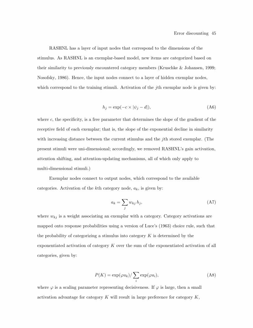
Error discounting 45

RASHNL has a layer of input nodes that correspond to the dimensions of the

stimulus. As RASHNL is an exemplar-based model, new items are categorized based on

their similarity to previously encountered category members (Kruschke & Johansen, 1999;

Nosofsky, 1986). Hence, the input nodes connect to a layer of hidden exemplar nodes,

which correspond to the training stimuli. Activation of the jth exemplar node is given by:

hj = exp(−c× |ψj − d|), (A6)

where c, the specificity, is a free parameter that determines the slope of the gradient of the

receptive field of each exemplar; that is, the slope of the exponential decline in similarity

with increasing distance between the current stimulus and the jth stored exemplar. (The

present stimuli were uni-dimensional; accordingly, we removed RASHNL’s gain activation,

attention shifting, and attention-updating mechanisms, all of which only apply to

multi-dimensional stimuli.)

Exemplar nodes connect to output nodes, which correspond to the available

categories. Activation of the kth category node, ak, is given by:

ak =∑j

wkj hj , (A7)

where wkj is a weight associating an exemplar with a category. Category activations are

mapped onto response probabilities using a version of Luce’s (1963) choice rule, such that

the probability of categorizing a stimulus into category K is determined by the

exponentiated activation of category K over the sum of the exponentiated activation of all

categories, given by:

P (K) = exp(ϕak)/∑i

exp(ϕai), (A8)

where ϕ is a scaling parameter representing decisiveness. If ϕ is large, then a small

activation advantage for category K will result in large preference for category K,

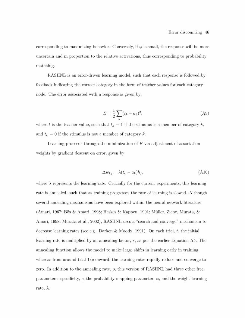
Error discounting 46

corresponding to maximizing behavior. Conversely, if ϕ is small, the response will be more

uncertain and in proportion to the relative activations, thus corresponding to probability

matching.

RASHNL is an error-driven learning model, such that each response is followed by

feedback indicating the correct category in the form of teacher values for each category

node. The error associated with a response is given by:

E =12

∑k

(tk − ak)2, (A9)

where t is the teacher value, such that tk = 1 if the stimulus is a member of category k,

and tk = 0 if the stimulus is not a member of category k.

Learning proceeds through the minimization of E via adjustment of association

weights by gradient descent on error, given by:

∆wkj = λ(tk − ak)hj , (A10)

where λ represents the learning rate. Crucially for the current experiments, this learning

rate is annealed, such that as training progresses the rate of learning is slowed. Although

several annealing mechanisms have been explored within the neural network literature

(Amari, 1967; Bos & Amari, 1998; Heskes & Kappen, 1991; Muller, Ziehe, Murata, &

Amari, 1998; Murata et al., 2002), RASHNL uses a “search and converge” mechanism to

decrease learning rates (see e.g., Darken & Moody, 1991). On each trial, t, the initial

learning rate is multiplied by an annealing factor, r, as per the earlier Equation A5. The

annealing function allows the model to make large shifts in learning early in training,

whereas from around trial 1/ρ onward, the learning rates rapidly reduce and converge to

zero. In addition to the annealing rate, ρ, this version of RASHNL had three other free

parameters: specificity, c, the probability-mapping parameter, ϕ, and the weight-learning

rate, λ.

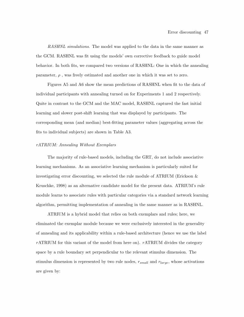
Error discounting 47

RASHNL simulations. The model was applied to the data in the same manner as

the GCM. RASHNL was fit using the models’ own corrective feedback to guide model

behavior. In both fits, we compared two versions of RASHNL: One in which the annealing

parameter, ρ , was freely estimated and another one in which it was set to zero.

Figures A5 and A6 show the mean predictions of RASHNL when fit to the data of

individual participants with annealing turned on for Experiments 1 and 2 respectively.

Quite in contrast to the GCM and the MAC model, RASHNL captured the fast initial

learning and slower post-shift learning that was displayed by participants. The

corresponding mean (and median) best-fitting parameter values (aggregating across the

fits to individual subjects) are shown in Table A3.

rATRIUM: Annealing Without Exemplars

The majority of rule-based models, including the GRT, do not include associative

learning mechanisms. As an associative learning mechanism is particularly suited for

investigating error discounting, we selected the rule module of ATRIUM (Erickson &

Kruschke, 1998) as an alternative candidate model for the present data. ATRIUM’s rule

module learns to associate rules with particular categories via a standard network learning

algorithm, permitting implementation of annealing in the same manner as in RASHNL.

ATRIUM is a hybrid model that relies on both exemplars and rules; here, we

eliminated the exemplar module because we were exclusively interested in the generality

of annealing and its applicability within a rule-based architecture (hence we use the label

rATRIUM for this variant of the model from here on). rATRIUM divides the category

space by a rule boundary set perpendicular to the relevant stimulus dimension. The

stimulus dimension is represented by two rule nodes, rsmall and rlarge, whose activations

are given by:

Error discounting 48

rsmall = 1− 11 + exp[−µ(d+ β)]

, (A11)

and by:

rlarge =1

1 + exp[−µ(d+ β)], (A12)

where d represents the value of a given item on the stimulus dimension. Each of these rule

nodes forms a sigmoid threshold function, centered on the rule boundary, such that larger

dimensional inputs will result in higher activation of the large rule node, while smaller

dimensional inputs will result in a higher activation of the small rule node. The parameter

µ represents the gain of the sigmoid (i.e., its steepness), and thus controls the level of

perceptual noise (or its equivalent) as dimensional values approach the rule boundary.

Large values of µ result in stimuli close to the rule boundary being more confusable. The

parameter β controls the position of the rule boundary.

The rule nodes are connected to output nodes that correspond to the possible

category selections. The activation of output nodes, ak, for each category, k, is calculated

as the sum of the activations of the small and large rule nodes, given by:

ak = wklargerlarge + wksmall

rsmall, (A13)

where the activation is moderated by the learned association weights, wk, between the rule

and output nodes. As in RASHNL, the association weights are updated by minimizing

mean square error during learning:

∆wkj = λ(tk − ak)rj , (A14)

where λ is a freely estimated parameter which controls the rate of learning. Finally,

output activations are converted into probabilities as in Equation A8 in RASHNL.

Error discounting 49

For present purposes, the annealing mechanism from RASHNL, given in

Equation A5, was imported into rATRIUM: Thus, an annealing rate, ρ, controlled the

rate at which the weight learning rate, λ, was adjusted on successive trials.

In summary, the model has four free parameters: A gain constant, µ, which sets the

standard deviation of the perceptual noise; a scaling constant, ϕ, which maps output

probabilities to participant responses; the annealing rate, ρ; and learning rate, λ.

The model was fit in the same manor as the fits with RASHNL. Figures A7 and A8

show the fits of rATRIUM to Experiment 1 and Experiment 2 respectively. Like

RASHNL, rATRIUM provided a good fit to the data. As shown in the figures, the model

closely tracked the behavior of the participants throughout training.

Fit Statistics

In Craig et al. (submitted), a series of fit statistics were used to compare the fits of

the four models, viz. AIC (Akaike Information Criterion; Akaike, 1974) and wi(AIC) (AIC

weights; Wagenmakers & Farrell, 2004), and BIC (Bayesian Information Criterion) and

wi(BIC) (BIC weights; Wagenmakers & Farrell, 2004) to compare the models. AIC and

BIC adjust for model complexity and flexibility. When corrected for small sample sizes,

the AIC (AICc) is given by:

AICc = −2 lnL+ 2V +2V (V + 1)n− V − 1

, (A15)

where L is the maximum likelihood for the given model with V free parameters taken over

n observations. The corrected AIC is recommended for use of samples where the ratio of

data points to parameters is less than 40. The AIC thus combines two sources of

information: Lack of fit (represented by the log likelihood) and a penalty term for model

complexity (represented by the second and third terms in the above equation). The BIC is

given by:

BIC = −2 lnL+ V lnn. (A16)

Error discounting 50

Unlike AIC, whose penalty relies on the number of parameters only, the BIC

additionally penalizes models based on the number of data points being fitted.

AICc and BIC values were converted into AIC and BIC weights (Wagenmakers &

Farrell, 2004). The wi(AIC), and wi(BIC), represent the conditional probabilities that the

model Mi is the best of the set of models being compared.

In Craig et al. (submitted), a likelihood-ratio test (Lamberts, 1997) was used to

determine whether the loss of fit associated with removal of error discounting, by setting ρ

to zero, was statistically significant. The likelihood-ratio test is given by:

χ2 = −2[lnL(restricted)− lnL(general)], (A17)

where lnL(general) is the log-likelihood of the version of a model that includes annealing

(i.e., ρ > 0), whereas lnL(restricted) is the log-likelihood of the restricted version of a

model, with annealing set to zero.

Error discounting 51

Author Note

Preparation of this paper was facilitated by a Discovery Grant from the Australian

Research Council and an Australian Professorial Fellowship to the second author. The

first and third authors were supported by Jean Rogerson Scholarships. Additionally, the

third author was supported by an Australian Postgraduate Scholarship and an NIH-NIMH

training grant #:T32 MH019879-14. We wish to thanks Charles Hanich for assisting with

data collection and Gordon Brown for his comments on an earlier version of this

manuscript. Address correspondence to the second author at the School of Psychology,

University of Western Australia, Crawley, W.A. 6009, Australia. Electronic mail may be

sent to lewan@psy.uwa.edu.au. Web page: http://www.cogsciwa.com.

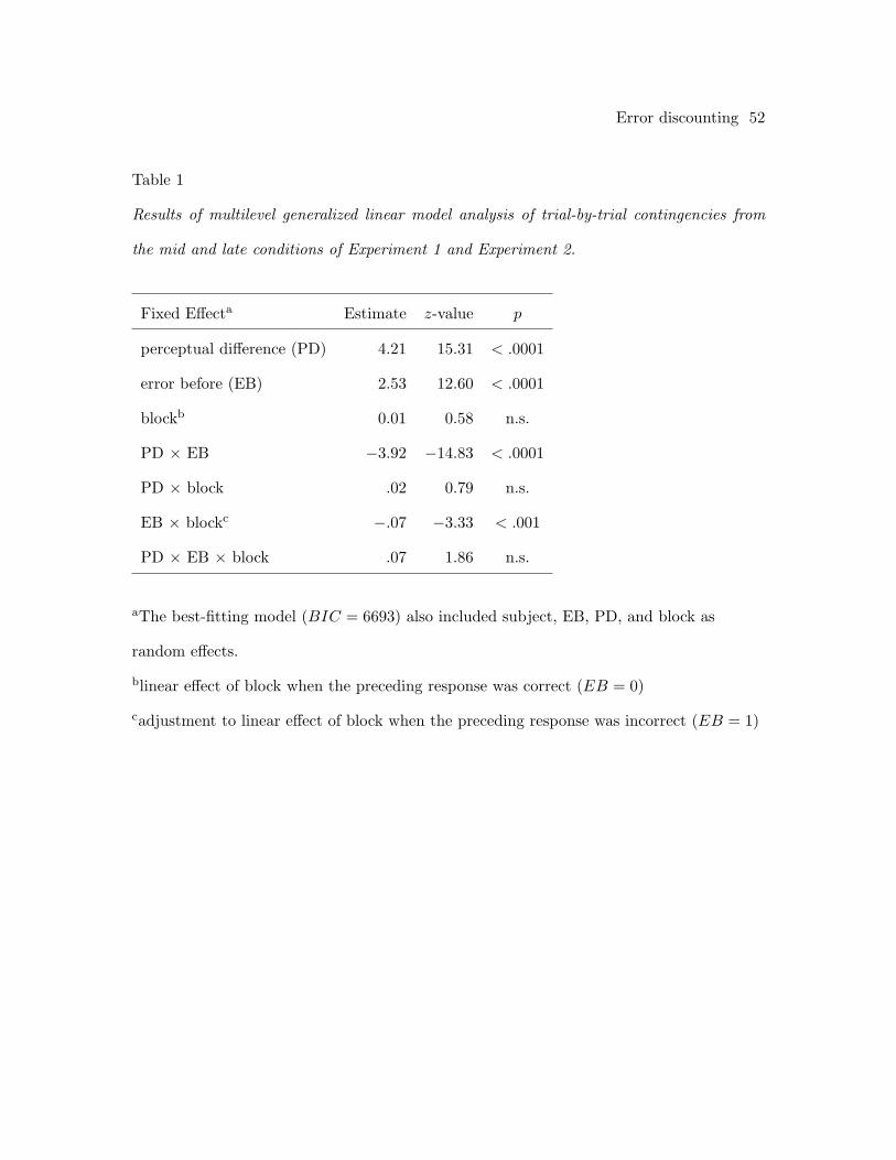
Error discounting 52

Table 1

Results of multilevel generalized linear model analysis of trial-by-trial contingencies from

the mid and late conditions of Experiment 1 and Experiment 2.

Fixed Effecta Estimate z-value p

perceptual difference (PD) 4.21 15.31 < .0001

error before (EB) 2.53 12.60 < .0001

blockb 0.01 0.58 n.s.

PD × EB −3.92 −14.83 < .0001

PD × block .02 0.79 n.s.

EB × blockc −.07 −3.33 < .001

PD × EB × block .07 1.86 n.s.

aThe best-fitting model (BIC = 6693) also included subject, EB, PD, and block as

random effects.

blinear effect of block when the preceding response was correct (EB = 0)

cadjustment to linear effect of block when the preceding response was incorrect (EB = 1)

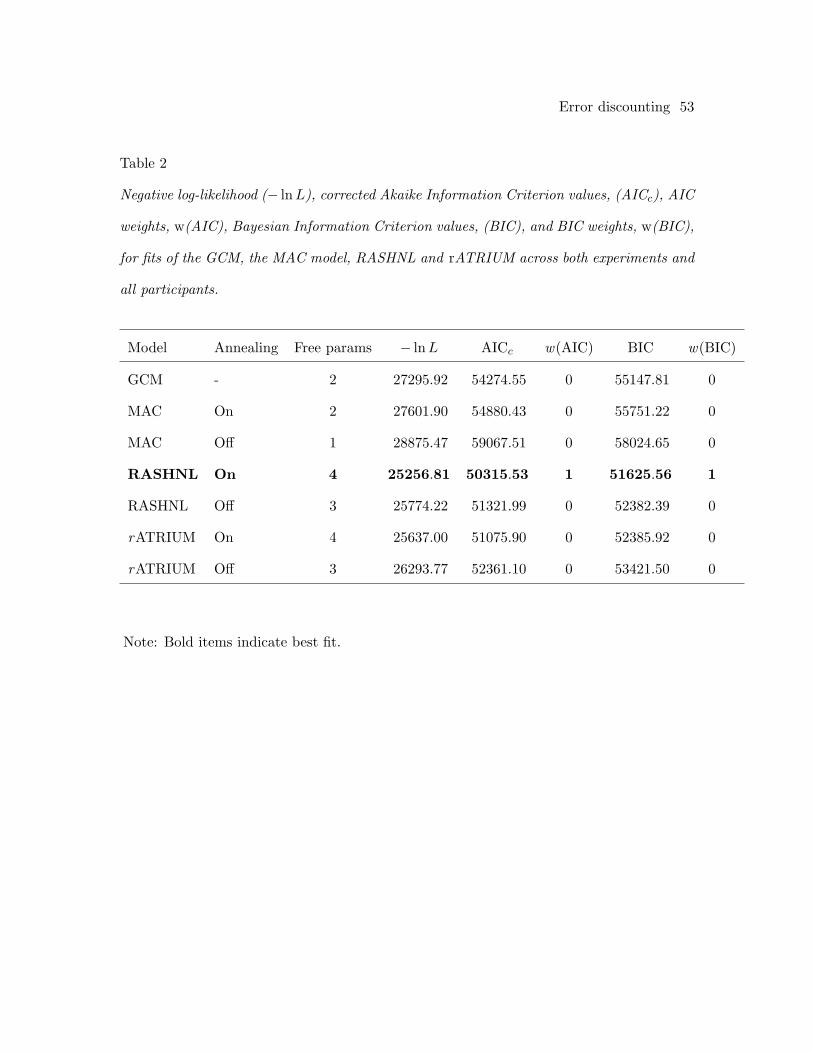
Error discounting 53

Table 2

Negative log-likelihood (− lnL), corrected Akaike Information Criterion values, (AICc), AIC

weights, w(AIC), Bayesian Information Criterion values, (BIC), and BIC weights, w(BIC),

for fits of the GCM, the MAC model, RASHNL and rATRIUM across both experiments and

all participants.

Model Annealing Free params − lnL AICc w(AIC) BIC w(BIC)

GCM - 2 27295.92 54274.55 0 55147.81 0

MAC On 2 27601.90 54880.43 0 55751.22 0

MAC Off 1 28875.47 59067.51 0 58024.65 0

RASHNL On 4 25256.81 50315.53 1 51625.56 1

RASHNL Off 3 25774.22 51321.99 0 52382.39 0

rATRIUM On 4 25637.00 51075.90 0 52385.92 0

rATRIUM Off 3 26293.77 52361.10 0 53421.50 0

Note: Bold items indicate best fit.

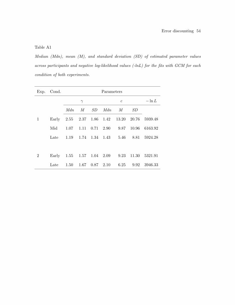
Error discounting 54

Table A1

Median (Mdn), mean (M), and standard deviation (SD) of estimated parameter values

across participants and negative log-likelihood values (-lnL) for the fits with GCM for each

condition of both experiments.

Exp. Cond. Parameters

γ c − lnL

Mdn M SD Mdn M SD

1 Early 2.55 2.37 1.86 1.42 13.20 20.76 5939.48

Mid 1.07 1.11 0.71 2.90 9.87 10.96 6163.92

Late 1.19 1.74 1.34 1.43 5.46 8.81 5924.28

2 Early 1.55 1.57 1.04 2.09 9.23 11.30 5321.91

Late 1.50 1.67 0.87 2.10 6.25 9.92 3946.33

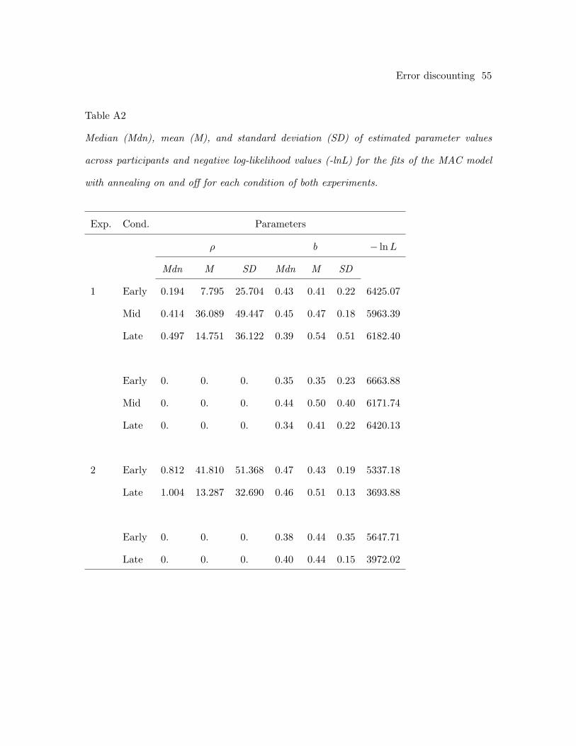
Error discounting 55

Table A2

Median (Mdn), mean (M), and standard deviation (SD) of estimated parameter values

across participants and negative log-likelihood values (-lnL) for the fits of the MAC model

with annealing on and off for each condition of both experiments.

Exp. Cond. Parameters

ρ b − lnL

Mdn M SD Mdn M SD

1 Early 0.194 7.795 25.704 0.43 0.41 0.22 6425.07

Mid 0.414 36.089 49.447 0.45 0.47 0.18 5963.39

Late 0.497 14.751 36.122 0.39 0.54 0.51 6182.40

Early 0. 0. 0. 0.35 0.35 0.23 6663.88

Mid 0. 0. 0. 0.44 0.50 0.40 6171.74

Late 0. 0. 0. 0.34 0.41 0.22 6420.13

2 Early 0.812 41.810 51.368 0.47 0.43 0.19 5337.18

Late 1.004 13.287 32.690 0.46 0.51 0.13 3693.88

Early 0. 0. 0. 0.38 0.44 0.35 5647.71

Late 0. 0. 0. 0.40 0.44 0.15 3972.02

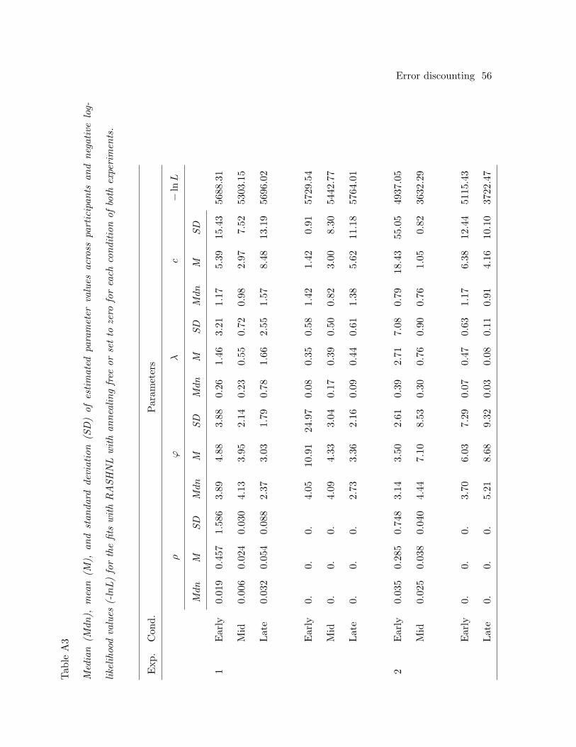
Error discounting 56T

able

A3

Med

ian

(Mdn

),m

ean

(M),

and

stan

dard

devi

atio

n(S

D)

ofes

tim

ated

para

met

erva

lues

acro

sspa

rtic

ipan

tsan

dne

gati

velo

g-

likel

ihoo

dva

lues

(-ln

L)

for

the

fits

wit

hR

ASH

NL

wit

han

neal

ing

free

orse

tto

zero

for

each

cond

itio

nof

both

expe

rim

ents

.

Exp

.C

ond.

Par

amet

ers

ρϕ

λc

−lnL

Mdn

MSD

Mdn

MSD

Mdn

MSD

Mdn

MSD

1E

arly

0.01

90.

457

1.58

63.

894.

883.

880.

261.

463.

211.

175.

3915

.43

5688

.31

Mid

0.00

60.

024

0.03

04.

133.

952.

140.

230.

550.

720.

982.

977.

5253

03.1

5

Lat

e0.

032

0.05

40.

088

2.37

3.03

1.79

0.78

1.66

2.55

1.57

8.48

13.1

956

96.0

2

Ear

ly0.

0.0.

4.05

10.9

124

.97

0.08

0.35

0.58

1.42

1.42

0.91

5729

.54

Mid

0.0.

0.4.

094.

333.

040.

170.

390.

500.

823.

008.

3054

42.7

7

Lat

e0.

0.0.

2.73

3.36

2.16

0.09

0.44

0.61

1.38

5.62

11.1

857

64.0

1

2E

arly

0.03

50.

285

0.74

83.

143.

502.

610.

392.

717.

080.

7918

.43

55.0

549

37.0

5

Mid

0.02

50.

038

0.04

04.

447.

108.

530.

300.

760.

900.

761.

050.

8236

32.2

9

Ear

ly0.

0.0.

3.70

6.03

7.29

0.07

0.47

0.63

1.17

6.38

12.4

451

15.4

3

Lat

e0.

0.0.

5.21

8.68

9.32

0.03

0.08

0.11

0.91

4.16

10.1

037

22.4

7

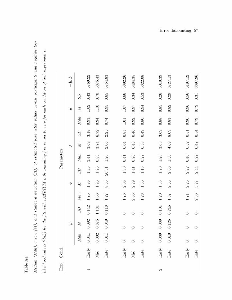
Error discounting 57T

able

A4

Med

ian

(Mdn

),m

ean

(M),

and

stan

dard

devi

atio

n(S

D)

ofes

tim

ated

para

met

erva

lues

acro

sspa

rtic

ipan

tsan

dne

gati

velo

g-

likel

ihoo

dva

lues

(-ln

L)

for

the

fits

wit

hrA

TR

IUM

wit

han

neal

ing

free

orse

tto

zero

for

each

cond

itio

nof

both

expe

rim

ents

.

Exp

.C

ond.

Par

amet

ers

ρϕ

λµ

−lnL

Mdn

MSD

Mdn

MSD

Mdn

MSD

Mdn

MSD

1E

arly

0.04

10.

092

0.14

21.

751.

981.

833.

413.

693.

180.

931.

020.

4357

69.2

2

Mid

0.00

20.

375

1.18

11.

661.

961.

260.

883.

746.

720.

941.

100.

7053

75.4

3

Lat

e0.

011

0.04

90.

118

1.27

8.65

26.3

11.

202.

062.

250.

740.

950.

6557

54.8

3

Ear

ly0.

0.0.

1.76

2.08

1.80

0.41

0.64

0.83

1.01

1.07

0.66

5892

.26

Mid

0.0.

0.2.

552.

291.

410.

260.

480.

460.

920.

970.

3454

84.3

5

Lat

e0.

0.0.

1.28

1.66

1.18

0.27

0.38

0.49

0.80

0.94

0.53

5822

.08

2E

arly

0.03

90.

089

0.10

11.

201.

531.

701.

283.

683.

690.

880.

850.

2650

10.3

9

Lat

e0.

019

0.12

60.

246

1.87

2.65

2.06

1.30

4.69

8.09

0.83

0.82

0.29

3727

.13

Ear

ly0.

0.0.

1.71

2.25

2.22

0.46

0.52

0.51

0.90

0.96

0.56

5197

.12

Lat

e0.

0.0.

2.86

3.27

2.44

0.22

0.47

0.54

0.79

0.79

0.31

3897

.96

Error discounting 58

Figure Captions

Figure 1. Probability of responding with category A for each of the training items across

training blocks for early, mid, and late conditions in Experiment 1. The legend identifies

each item’s reinforcement probabilities, P (A|j), before and after the shift.

Figure 2. Observed slope through response probabilities across all 4 training items in

Experiment 1 (solid lines) and objective slopes (dotted lines). Error bars indicate 95%

confidence intervals. The three panels show the early (top), mid (middle), and late

(bottom) condition, respectively.

Figure 3. Decisional-recency analysis for all conditions in Experiment 1. The probability

of shifting the response from one category to the other on trial n is shown as a function of

whether the response on trial n− 1 was an error or correct. The top panel is for two

identical stimuli in succession and the bottom panel is for two maximally dissimilar

stimuli following each other. The smooth lines are based on locally-weighted regression

(lowess). See text for details of alignment of conditions.

Figure 4. Observed slope through response probabilities across all 4 training items in

Experiment 2 (solid lines) and objective slopes (dotted lines). Error bars indicate 95%

confidence intervals. The two panels show the early (top) and late (bottom) condition,

respectively.

Figure 5. Decisional-recency analysis for all conditions in Experiment 2. The probability

of shifting the response from one category to the other on trial n is shown as a function of

whether the response on trial n− 1 was an error or correct. The top panel is for two

identical stimuli in succession and the bottom panel is for two maximally dissimilar

stimuli following each other. The smooth lines are based on locally-weighted regression

(lowess). See text for details of alignment of conditions.

Error discounting 59

Figure A1. Observed slopes through response probabilities across all 4 training items in

Experiment 1 (solid lines and error bars), slopes predicted by GCM (solid lines and open

circles), and objective slopes (dotted lines). Error bars indicate 95% confidence intervals.

The three panels show the early (top), mid (middle), and late (bottom) condition,

respectively.

Figure A2. Observed slopes through response probabilities across all 4 training items in

Experiment 2 (solid lines and error bars), slopes predicted by GCM (solid lines and open

circles), and objective slopes (dotted lines). Error bars indicate 95% confidence intervals.

The two panels show the early (top) and late (bottom) condition, respectively.

Figure A3. Observed slopes through response probabilities across all 4 training items in

Experiment 1 (solid lines and error bars), slopes predicted by the MAC model (solid lines

and open circles), and objective slopes (dotted lines). Error bars indicate 95% confidence

intervals. The three panels show the early (top), mid (middle) and late (bottom)

condition, respectively.

Figure A4. Observed slopes through response probabilities across all 4 training items in

Experiment 2 (solid lines and error bars), slopes predicted by the MAC model (solid lines

and open circles), and objective slopes (dotted lines). Error bars indicate 95% confidence

intervals. The two panels show the early (top) and late (bottom) condition, respectively.

Figure A5. Observed slopes through response probabilities across all 4 training items in

Experiment 1 (solid lines and error bars), slopes predicted by RASHNL (solid lines and

open circles), and objective slopes (dotted lines). RASHNL’s predictions were obtained

with the annealing parameter, ρ, being freely estimated. Error bars indicate 95%

confidence intervals. The three panels show the early (top), mid (middle), and late

(bottom) condition, respectively.

Error discounting 60

Figure A6. Observed slopes through response probabilities across all 4 training items in

Experiment 2 (solid lines and error bars), slopes predicted by RASHNL (solid lines and

open circles), and objective slopes (dotted lines). RASHNL’s predictions were obtained

with the annealing parameter, ρ, being freely estimated. Error bars indicate 95%

confidence intervals. The two panels show the early (top) and late (bottom) condition,

respectively.

Figure A7. Observed slopes through response probabilities across all 4 training items in

Experiment 1 (solid lines and error bars), slopes predicted by rATRIUM (solid lines and

open circles), and objective slopes (dotted lines). rATRIUM’s predictions were obtained

with the annealing parameter, ρ, being freely estimated. Error bars indicate 95%

confidence intervals. The three panels show the early (top), mid (middle), and late

(bottom) condition, respectively.

Figure A8. Observed slopes through response probabilities across all 4 training items in

Experiment 2 (solid lines and error bars), slopes predicted by rATRIUM (solid lines and

open circles), and objective slopes (dotted lines). rATRIUM’s predictions were obtained

with the annealing parameter, ρ, being freely estimated. Error bars indicate 95%

confidence intervals. The two panels show the early (top) and late (bottom) condition,

respectively.

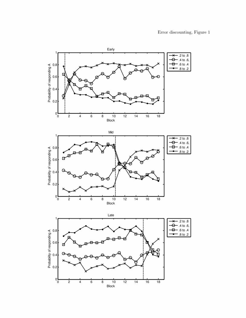
Error discounting, Figure 1

0 2 4 6 8 10 12 14 16 180

0.2

0.4

0.6

0.8

1

Block

Pro

babili

ty o

f re

spondin

g A

Early

.2 to .8

.4 to .6,

.6 to .4

.8 to .2

0 2 4 6 8 10 12 14 16 180

0.2

0.4

0.6

0.8

1

Block

Pro

babili

ty o

f re

spondin

g A

Mid

.2 to .8

.4 to .6,

.6 to .4

.8 to .2

0 2 4 6 8 10 12 14 16 180

0.2

0.4

0.6

0.8

1

Block

Pro

babili

ty o

f re

spondin

g A

Late

.2 to .8

.4 to .6,

.6 to .4

.8 to .2

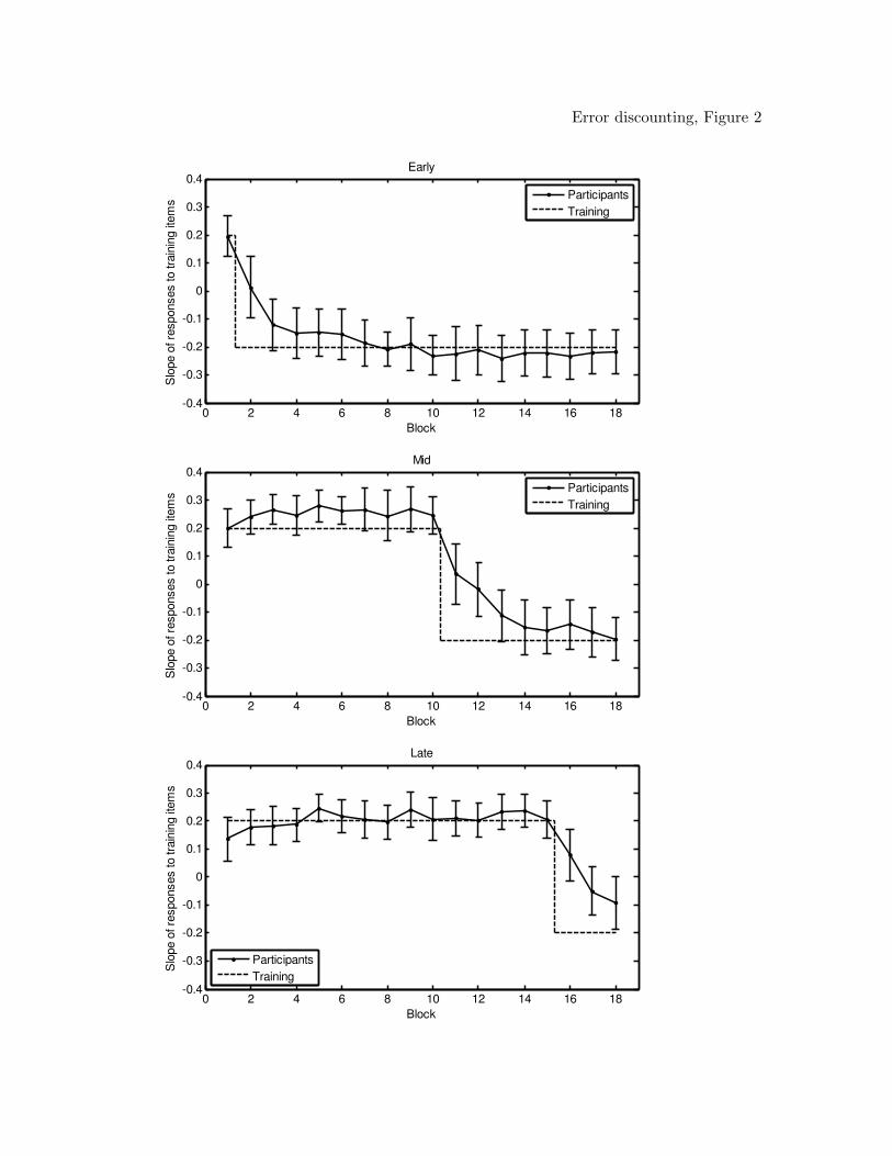
Error discounting, Figure 2

0 2 4 6 8 10 12 14 16 18-0.4

-0.3

-0.2

-0.1

0

0.1

0.2

0.3

0.4

Block

Slo

pe o

f re

sponses to tra

inin

g it

em

sEarly

Participants

Training

0 2 4 6 8 10 12 14 16 18-0.4

-0.3

-0.2

-0.1

0

0.1

0.2

0.3

0.4

Block

Slo

pe o

f re

sponses to tra

inin

g it

em

s

Mid

Participants

Training

0 2 4 6 8 10 12 14 16 18-0.4

-0.3

-0.2

-0.1

0

0.1

0.2

0.3

0.4

Block

Slo

pe o

f re

sponses to tra

inin

g it

em

s

Late

Participants

Training

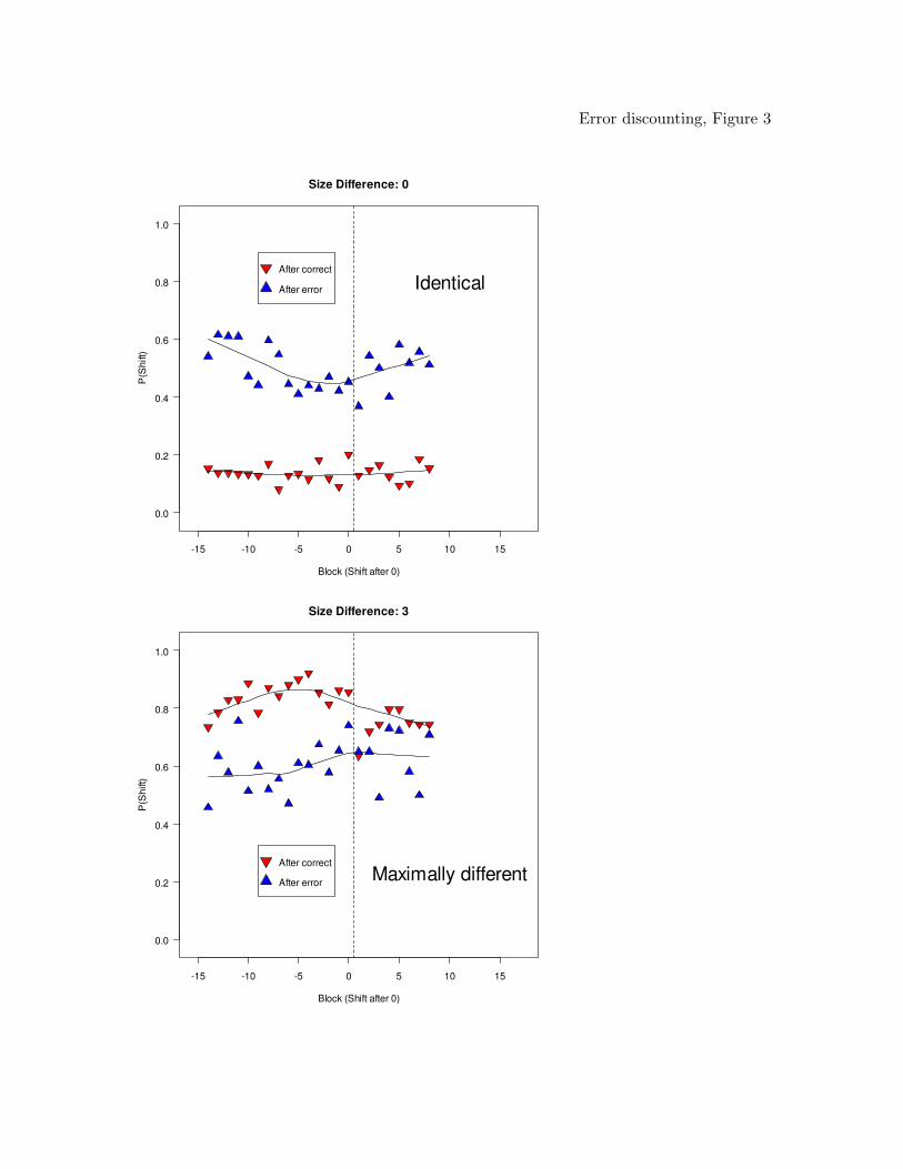
Error discounting, Figure 3

-15 -10 -5 0 5 10 15

0.0

0.2

0.4

0.6

0.8

1.0

Block (Shift after 0)

P(S

hift)

After correct

After error

Size Difference: 0

Identical

-15 -10 -5 0 5 10 15

0.0

0.2

0.4

0.6

0.8

1.0

Block (Shift after 0)

P(S

hift)

After correct

After error

Size Difference: 3

Maximally different

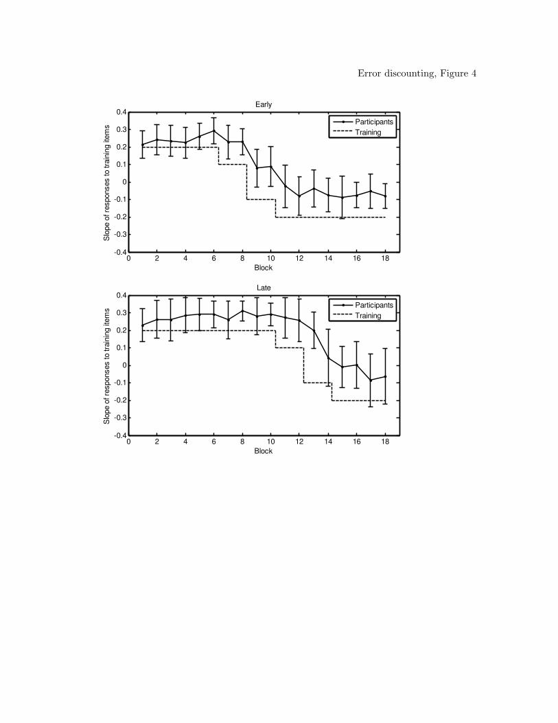
Error discounting, Figure 4

0 2 4 6 8 10 12 14 16 18-0.4

-0.3

-0.2

-0.1

0

0.1

0.2

0.3

0.4

Block

Slo

pe o

f re

sponses to tra

inin

g it

em

sEarly

Participants

Training

0 2 4 6 8 10 12 14 16 18-0.4

-0.3

-0.2

-0.1

0

0.1

0.2

0.3

0.4

Block

Slo

pe o

f re

sponses to tra

inin

g it

em

s

Late

Participants

Training

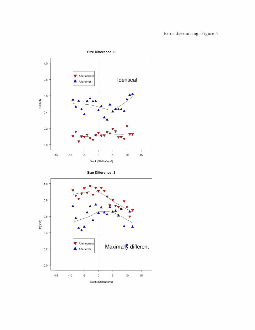
Error discounting, Figure 5

-15 -10 -5 0 5 10 15

0.0

0.2

0.4

0.6

0.8

1.0

Block (Shift after 0)

P(S

hift)

After correct

After error

Size Difference: 0

Identical

-15 -10 -5 0 5 10 15

0.0

0.2

0.4

0.6

0.8

1.0

Block (Shift after 0)

P(S

hift)

After correct

After error

Size Difference: 3

Maximally different

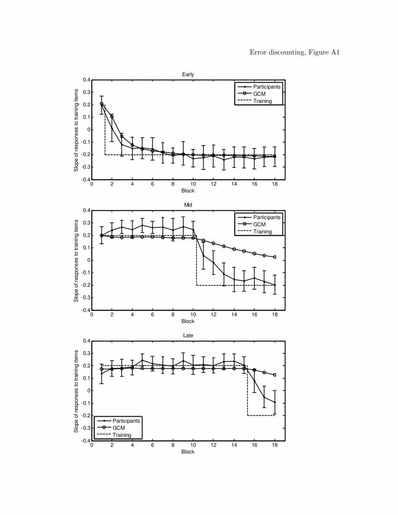
Error discounting, Figure A1

0 2 4 6 8 10 12 14 16 18-0.4

-0.3

-0.2

-0.1

0

0.1

0.2

0.3

0.4

Block

Slo

pe o

f re

sponses to tra

inin

g it

em

sEarly

Participants

GCM

Training

0 2 4 6 8 10 12 14 16 18-0.4

-0.3

-0.2

-0.1

0

0.1

0.2

0.3

0.4

Block

Slo

pe o

f re

sponses to tra

inin

g it

em

s

Mid

Participants

GCM

Training

0 2 4 6 8 10 12 14 16 18-0.4

-0.3

-0.2

-0.1

0

0.1

0.2

0.3

0.4

Block

Slo

pe o

f re

sponses to tra

inin

g it

em

s

Late

Participants

GCM

Training

Error discounting, Figure A2

0 2 4 6 8 10 12 14 16 18-0.4

-0.3

-0.2

-0.1

0

0.1

0.2

0.3

0.4

Block

Slo

pe o

f re

sponses to tra

inin

g it

em

sEarly

Participants

GCM

Training

0 2 4 6 8 10 12 14 16 18-0.4

-0.3

-0.2

-0.1

0

0.1

0.2

0.3

0.4

Block

Slo

pe o

f re

sponses to tra

inin

g it

em

s

Late

Participants

GCM

Training

Error discounting, Figure A3

0 2 4 6 8 10 12 14 16 18-0.4

-0.3

-0.2

-0.1

0

0.1

0.2

0.3

0.4

Block

Slo

pe o

f re

sponses to tra

inin

g it

em

sEarly

Participants

MAC

Training

0 2 4 6 8 10 12 14 16 18-0.4

-0.3

-0.2

-0.1

0

0.1

0.2

0.3

0.4

Block

Slo

pe o

f re

sponses to tra

inin

g it

em

s

Mid

Participants

MAC

Training

0 2 4 6 8 10 12 14 16 18-0.4

-0.3

-0.2

-0.1

0

0.1

0.2

0.3

0.4

Block

Slo

pe o

f re

sponses to tra

inin

g it

em

s

Late

Participants

MAC

Training

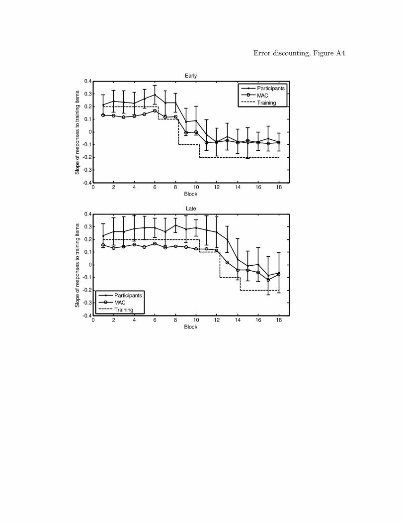
Error discounting, Figure A4

0 2 4 6 8 10 12 14 16 18-0.4

-0.3

-0.2

-0.1

0

0.1

0.2

0.3

0.4

Block

Slo

pe o

f re

sponses to tra

inin

g it

em

sEarly

Participants

MAC

Training

0 2 4 6 8 10 12 14 16 18-0.4

-0.3

-0.2

-0.1

0

0.1

0.2

0.3

0.4

Block

Slo

pe o

f re

sponses to tra

inin

g it

em

s

Late

Participants

MAC

Training

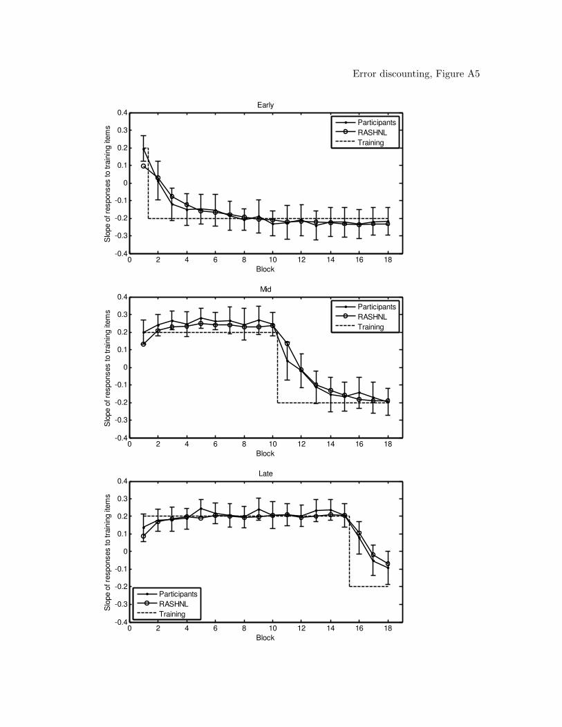
Error discounting, Figure A5

0 2 4 6 8 10 12 14 16 18-0.4

-0.3

-0.2

-0.1

0

0.1

0.2

0.3

0.4

Block

Slo

pe o

f re

sponses to tra

inin

g it

em

sEarly

Participants

RASHNL

Training

0 2 4 6 8 10 12 14 16 18-0.4

-0.3

-0.2

-0.1

0

0.1

0.2

0.3

0.4

Block

Slo

pe o

f re

sponses to tra

inin

g it

em

s

Mid

Participants

RASHNL

Training

0 2 4 6 8 10 12 14 16 18-0.4

-0.3

-0.2

-0.1

0

0.1

0.2

0.3

0.4

Block

Slo

pe o

f re

sponses to tra

inin

g it

em

s

Late

Participants

RASHNL

Training

Error discounting, Figure A6

0 2 4 6 8 10 12 14 16 18-0.4

-0.3

-0.2

-0.1

0

0.1

0.2

0.3

0.4

Block

Slo

pe o

f re

sponses to tra

inin

g it

em

sEarly

Participants

RASHNL

Training

0 2 4 6 8 10 12 14 16 18-0.4

-0.3

-0.2

-0.1

0

0.1

0.2

0.3

0.4

Block

Slo

pe o

f re

sponses to tra

inin

g it

em

s

Late

Participants

RASHNL

Training

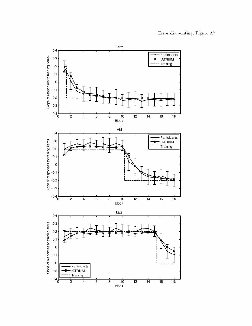
Error discounting, Figure A7

0 2 4 6 8 10 12 14 16 18-0.4

-0.3

-0.2

-0.1

0

0.1

0.2

0.3

0.4

Block

Slo

pe o

f re

sponses to tra

inin

g it

em

sEarly

Participants

rATRIUM

Training

0 2 4 6 8 10 12 14 16 18-0.4

-0.3

-0.2

-0.1

0

0.1

0.2

0.3

0.4

Block

Slo

pe o

f re

sponses to tra

inin

g it

em

s

Mid

Participants

rATRIUM

Training

0 2 4 6 8 10 12 14 16 18-0.4

-0.3

-0.2

-0.1

0

0.1

0.2

0.3

0.4

Block

Slo

pe o

f re

sponses to tra

inin

g it

em

s

Late

Participants

rATRIUM

Training

Error discounting, Figure A8

0 2 4 6 8 10 12 14 16 18-0.4

-0.3

-0.2

-0.1

0

0.1

0.2

0.3

0.4

Block

Slo

pe o

f re

sponses to tra

inin

g it

em

sEarly

Participants

rATRIUM

Training

0 2 4 6 8 10 12 14 16 18-0.4

-0.3

-0.2

-0.1

0

0.1

0.2

0.3

0.4

Block

Slo

pe o

f re

sponses to tra

inin

g it

em

s

Late

Participants

rATRIUM

Training