Error-Detection Codes:Algorithms and Fast Implementation

Gam D. Nguyen

Abstract—Binary CRCs are very effective for error detection, but their software implementation is not very efficient. Thus, many binary

non-CRC codes (which are not as strong as CRCs, but can be more efficiently implemented in software) are proposed as alternatives

to CRCs. The non-CRC codes include WSC, CXOR, one’s-complement checksum, Fletcher checksum, and block-parity code. In this

paper, we present a general algorithm for constructing a family of binary error-detection codes. This family is large because it contains

all these non-CRC codes, CRCs, perfect codes, as well as other linear and nonlinear codes. In addition to unifying these apparently

disparate codes, our algorithm also generates some non-CRC codes that have minimum distance 4 (like CRCs) and efficient software

implementation.

Index Terms—Fast error-detection code, Hamming code, CRC, checksum.

�

1 INTRODUCTION

EFFICIENT implementation of reliable error-protectionalgorithms plays a vital role in digital communication

and storage because channel noise and system malfunc-tion introduce errors in received and retrieved messages.Here, we focus on binary error-detection codes that havelow overhead and minimum distance d � 4. Popularerror-detection codes used in practice include CRCs thatare generated by binary polynomials such as X16 þX15 þX2 þ 1 (called CRC-16) and X16 þX12 þX5 þ 1 (calledCRC-CCITT).

An h-bit CRC generated by GðXÞ ¼ ðX þ 1ÞP ðXÞ, whereP ðXÞ is a primitive polynomial of degree h� 1, has thefollowing desirable properties [1]. The CRC has maximumcodeword length of 2h�1 � 1 bits and minimum distanced ¼ 4, i.e., all double and odd errors are detected. This codealso detects any error burst of length h bits or less, i.e., itsburst-error-detecting capability is b ¼ h. The guaranteederror-detection capability of this h-bit CRC is nearly optimalbecause its maximum codeword length almost meets theupper bound 2h�1 and its burst-error-detecting capabilitymeets the upper bound h. The CRC is also efficientlyimplemented by special-purpose shift-register hardware.

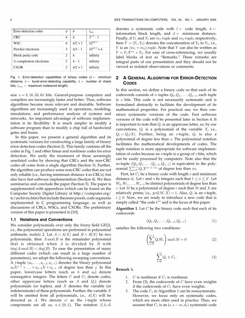
Although CRCs have nearly optimal properties andefficient hardware implementation, many binary non-CRCcodes are proposed as alternatives to CRCs. These codes,developed over many years and often considered asunrelated to each other, do not have the CRC’s desirableproperties. Such non-CRC codes include weighted sumcode (WSC), Fletcher checksum (used in ISO), one’s-complement checksum (used in Internet), circular-shiftand exclusive-OR checksum (CXOR), and block-parity code(Fig. 1). See [4], [5], [9], [14] for implementation and

performance comparisons of CRCs and these non-CRCcodes. Perhaps the key reason for the appearance of thenon-CRC codes is that CRCs are not very efficientlyimplemented in software. Software complexity refers tothe number of programming operations and hardwarecomplexity refers to the number of gates required for codeimplementation. Investigations reported in [4], [9] indicatethat software processing of CRCs is slower than that of thenon-CRC codes. Thus, it is desirable to design error-detection codes that are reliable and of low complexity.One code is better than another if, for a fixed number ofcheck bits h, it has larger minimum distance d, larger burst-error-detecting capability b, longer maximum codewordlength lmax, and lower complexity.

An important performance measure of a code, which isnot addressed in this paper, is its probability of undetectederror. For the binary symmetric channel, this probability canbe expressed in terms of the weight distribution of the code.In general, the problem of computing the probability ofundetected error is NP-hard [7]. Some methods forcalculating or estimating this probability are given in [7].

Because the minimum distance d is often considered themost important parameter, Fig. 1 ranks CRC as the bestcode, WSC the second best, and so on. Although the WSC,Fletcher checksum, and CXOR are defined only for an evennumber of check bits h, both even and odd h can be used forthe other codes. The CRC, WSC, and Fletcher checksum canbe extended to have infinite length, but their minimumdistances all reduce to 2. Some discussions of burst-error-detecting capability b are given in Appendix C (which canbe found on the Computer Society Digital Library at http://computer.org/tc/archives.htm). In this paper, we focus oncode implementation by means of software. Becausecomputers can process information in blocks of bits (e.g.,bytes or words), codes having efficient software implemen-tation should also be processed in blocks of bits. Then, it isnatural to express code lengths in terms of the number ofblocks n and each block is s bits, i.e., the total number of bitsis ns. Most modern processors can efficiently handle block

IEEE TRANSACTIONS ON COMPUTERS, VOL. 54, NO. 1, JANUARY 2005 1

. The author is with the Information Technology Division, Naval ResearchLaboratory, Washington, DC 20375. E-mail: nguyen@itd.nrl.navy.mil.

Manuscript received 27 Mar. 2003; revised 26 Feb. 2004; accepted 30 July2004; published online 16 Nov. 2004.For information on obtaining reprints of this article, please send e-mail to:tc@computer.org, and reference IEEECS Log Number 118495.

U.S. Government Work Not Protected by U.S. Copyright

Report Documentation Page Form ApprovedOMB No. 0704-0188

Public reporting burden for the collection of information is estimated to average 1 hour per response, including the time for reviewing instructions, searching existing data sources, gathering andmaintaining the data needed, and completing and reviewing the collection of information. Send comments regarding this burden estimate or any other aspect of this collection of information,including suggestions for reducing this burden, to Washington Headquarters Services, Directorate for Information Operations and Reports, 1215 Jefferson Davis Highway, Suite 1204, ArlingtonVA 22202-4302. Respondents should be aware that notwithstanding any other provision of law, no person shall be subject to a penalty for failing to comply with a collection of information if itdoes not display a currently valid OMB control number.

1. REPORT DATE 26 FEB 2004 2. REPORT TYPE

3. DATES COVERED 00-00-2004 to 00-00-2004

4. TITLE AND SUBTITLE Error-Detection Codes: Algorithms and Fast Implementation

5a. CONTRACT NUMBER

5b. GRANT NUMBER

5c. PROGRAM ELEMENT NUMBER

6. AUTHOR(S) 5d. PROJECT NUMBER

5e. TASK NUMBER

5f. WORK UNIT NUMBER

7. PERFORMING ORGANIZATION NAME(S) AND ADDRESS(ES) Naval Research Laboratory,Information Technology Division,4555Overlook Avenue SW,Washington,DC,20375

8. PERFORMING ORGANIZATIONREPORT NUMBER

9. SPONSORING/MONITORING AGENCY NAME(S) AND ADDRESS(ES) 10. SPONSOR/MONITOR’S ACRONYM(S)

11. SPONSOR/MONITOR’S REPORT NUMBER(S)

12. DISTRIBUTION/AVAILABILITY STATEMENT Approved for public release; distribution unlimited

13. SUPPLEMENTARY NOTES

14. ABSTRACT see report

15. SUBJECT TERMS

16. SECURITY CLASSIFICATION OF: 17. LIMITATION OF ABSTRACT Same as

Report (SAR)

18. NUMBEROF PAGES

11

19a. NAME OFRESPONSIBLE PERSON

a. REPORT unclassified

b. ABSTRACT unclassified

c. THIS PAGE unclassified

Standard Form 298 (Rev. 8-98) Prescribed by ANSI Std Z39-18

size s ¼ 8; 16; 32; 64 bits. General-purpose computers andcompilers are increasingly faster and better. Thus, softwarealgorithms become more relevant and desirable. Softwarealgorithms are increasingly used in operations, modeling,simulations, and performance analysis of systems andnetworks. An important advantage of software implemen-tation is its flexibility: It is much simpler to modify asoftware program than to modify a chip full of hardwiredgates and buses.

In this paper, we present a general algorithm and itssystematic versions for constructing a large family of binaryerror-detection codes (Section 2). This family contains all thecodes in Fig. 1 and other linear and nonlinear codes for errordetection. We unify the treatment of these seeminglyunrelated codes by showing that CRCs and the non-CRCcodes all come from a single algorithm (Section 3). Further,the algorithm can produce some non-CRC codes that are notonly reliable (i.e., having minimum distance 4 as CRCs), butalso have fast software implementation (Section 4). We thensummarize and conclude the paper (Section 5). The paper issupplemented with appendices (which can be found on theComputer Society Digital Library at http://computer.org/tc/archives.htm) that include theoremproofs, code segmentsimplemented in C programming language, as well asdiscussions of CRCs, WSCs, and CXORs. The preliminaryversion of this paper is presented in [10].

1.1 Notations and Conventions

We consider polynomials over only the binary field GF(2),i.e., the polynomial operations are performed in polynomialarithmetic modulo 2. Let A ¼ AðXÞ and B ¼ BðXÞ be twopolynomials, then AmodB is the remainder polynomialthat is obtained when A is divided by B withdegðAmodBÞ < degðBÞ. To ease the presentation of manydifferent codes (which can result in a large number ofparameters), we adopt the following sweeping conventions.A j-tuple ða0; . . . ; aj�2; aj�1Þ denotes the binary polynomiala0X

j�1 þ . . .þ aj�2X þ aj�1 of degree less than j. In thispaper, lowercase letters (such as h and a0) denotenonnegative integers. The letters C and C1 denote codes,other uppercase letters (such as A and Qi) denotepolynomials (or tuples), and X denotes the variable (orindeterminate) of these polynomials. Further, the variableXwill be omitted from all polynomials, i.e., AðXÞ will bedenoted as A. We denote ui as the i-tuple whosecomponents are all us, u 2 f0; 1g. The notation ðl; k; dÞ

denotes a systematic code with l ¼ code length, k ¼information block length, and d ¼ minimum distance.Finally, if Y1 and Y2 are m1-tuple and m2-tuple, respectively,then Y ¼ ðY1; Y2Þ denotes the concatenation of Y2 to Y1, i.e.,Y is an ðm1 þm2Þ-tuple. Note that Y can also be written asY ¼ Y1X

m2 þ Y2. For ease of cross-referencing, we usuallylabel blocks of text as “Remarks.” These remarks areintegral parts of our presentation and they should not beviewed as isolated observations or comments.

2 A GENERAL ALGORITHM FOR ERROR-DETECTION

CODES

In this section, we define a binary code so that each of its

codewords consists of n tuples Q0; Q1; . . . ; Qn�1, each tuple

is s bits. This code is not necessarily systematic and is

formulated abstractly to facilitate the development of its

mathematical properties. For practical use, we then con-

struct systematic versions of the code. Fast software

versions of the code will be presented later in Section 4. It

is important to note that Qi is an uppercase letter, so, by our

conventions, Qi is a polynomial of the variable X, i.e.,

Qi ¼ QiðXÞ. Further, being an s-tuple, Qi is also a

polynomial of degree less than s. The polynomial notation

facilitates the mathematical developments of codes. The

tuple notation is more appropriate for software implemen-

tation of codes because an s-tuple is a group of s bits, which

can be easily processed by computers. Note also that the

ns-tuple ðQ0; Q1; . . . ; Qn�2; Qn�1Þ is equivalent to the poly-

nomialPn�1

i¼0 QiXðn�1�iÞs of degree less than ns.

First, let C1 be a binary code with length s and minimumdistance d1. Let r and n be integers such that 1 � n � 2r. LetW0;W1; . . . ;Wn�1 be distinct polynomials of degree less thanr. Let M be a polynomial of degree r such that M and X arerelatively prime, i.e., gcdðM;XÞ ¼ 1. Also, Qi is an s-tuple,i � 0. Now, we are ready to introduce a new code that issimply called “the code C” and is the focus of this paper.

Algorithm 1. Let C be the binary code such that each of itscodewords

ðQ0; Q1; . . . ; Qn�2; Qn�1Þ ð1Þ

satisfies the following two conditions:

Xn�1

i¼0

QiWi

!modM ¼ 0 ð2Þ

Xn�1

i¼0

Qi 2 C1: ð3Þ

Remark 1.

1. C is nonlinear if C1 is nonlinear.2. From (3), the codewords of C have even weights

if the codewords of C1 have even weights.3. The code C1 in Algorithm 1 can be nonsystematic.

However, we focus only on systematic codes,which are more often used in practice. Thus, weassume that C1 is an (s; s�m; d1Þ systematic code

2 IEEE TRANSACTIONS ON COMPUTERS, VOL. 54, NO. 1, JANUARY 2005

Fig. 1. Error-detection capabilities of binary codes (d ¼ minimum

distance, b ¼ burst-error-detecting capability, h ¼ number of check

bits, lmax ¼ maximum codeword length).

with m check bits, 0 � m � s. Let F be theencoder of C1. Then, each codeword of C1 isUXm þ F ðUÞ ¼ ðU; F ðUÞÞ, where U is an informa-tion ðs�mÞ-tuple and F ðUÞ is the correspondingcheck m-tuple.

4. In Algorithm 1, the weights W0;W1; . . . ;Wn�1 canbe chosen to be distinct polynomials of degreeless than r because 1 � n � 2r. However, Algo-rithm 1 can be extended to allow n > 2r, thenW0;W1; . . . ;Wn�1 will not always be distinct (seeSection 3 later).

5. All the codes considered in this paper are binarycodes, i.e., their codewords consist of digits 0 or 1.In particular, the code C is a binary code whosecodewords are ns bits. Computers can efficientlyprocess groups of bits. Thus, as seen in (1), eachns-bit codeword is grouped into n tuples, s bitseach. Note that this binary code C can also beviewed as a code in GFð2sÞ, i.e., as a code whosecodewords consist of n symbols, each symbolbelongs to GFð2sÞ. More generally, suppose thatns ¼ xy for some positive integers x and y, thenthis same binary code C can also be viewed as acode whose codewords consist of x symbols, eachsymbol belongs to GFð2yÞ. In the extreme case(x ¼ 1, y ¼ ns), the code C is also a code whosecodewords consist of only one symbol thatbelongs to GFð2nsÞ. Note that, when the samecode is viewed in different alphabets, theirrespective minimum distances can be very differ-ent. For example, consider the binary repetitioncode f0k; 1kg of length k > 1. When viewed as thebinary code over GF(2), this code has minimumdistance d ¼ k. But, when viewed in GFð2kÞ, thissame code has minimum distance d ¼ 1.

Let d1 and dC be the minimum distances of the binarycodes C1 and C, respectively, in Algorithm 1. We then havethe following theorem that is proven in Appendix A (whichcan be found on the Computer Society Digital Library athttp://computer.org/tc/archives.htm).

Theorem 1.

1. dC � 3 if d1 � 3.2. dC ¼ 4 if d1 � 4.

Example 1. Now, we illustrate Algorithm 1 by construct-ing a simple binary code C. Let s ¼ 4, m ¼ 3, r ¼ 2,and n ¼ 2r ¼ 4. Thus, each codeword of the code Cis a 16-tuple ðQ0; Q1; Q2; Q3Þ, where each Qi is a4-tuple. Let M ¼ X2 þX þ 1 be the modulating(primitive) polynomial. Let the weighting polynomialsin (2) be W0 ¼ X þ 1, W1 ¼ X, W2 ¼ 1, and W3 ¼ 0.Let C1 ¼ fð0; 0; 0; 0Þ; ð1; 1; 1; 1Þg, i.e., C1 is the ð4; 1; 4Þrepetition code. Now, we wish to specify the desiredcodeword ðQ0; Q1; Q2; Q3Þ. Let Q0 and Q1 be twoarbitrary 4-tuples. Then, Q2 and Q3 are determined asfollows: Let U1 and U2 be arbitrary 2-tuple and 1-tuple,respectively. Then, we define Q2 ¼ ðU1; P1Þ andQ3 ¼ ðU2; P2Þ, where P1 and P2 are determined as follows:F i r s t , c o m p u t e t h e c h e c k 2 - t u p l eP1 ¼ ðQ0W0 þQ1W1 þ U1X

2ÞmodM. Next, define

Y ¼ Q0 þQ1 þ ðU1X2 þ P1Þ þ U2X

3

¼ Q0 þQ1 þQ2 þ U2X3;

which is a 4-tuple. Thus, Y can be written asY ¼ Y1X

3 þ Y2 ¼ ðY1; Y2Þ, where Y1 is a 1-tuple and Y2

is a 3-tuple. Finally, we compute P2 ¼ Y2 þ ðY1; Y1; Y1Þ,which is a 3-tuple.

Now, we wi l l show tha t the codewordðQ0; Q1; Q2; Q3Þ ¼ ðQ0; Q1; U1; P1; U2; P2Þ satisfies (2) and( 3 ) i n A l g o r i t h m 1 . S i n c eP1 ¼ ðQ0W0 þQ1W1 þ U1X

2ÞmodM, we have

0 ¼ ðQ0W0 þQ1W1 þ U1X2 þ P1ÞmodM:

Then, 0 ¼ ðQ0W0 þQ1W1 þQ2W2 þQ3W3ÞmodM be-c a u s e Q2W2 ¼ U1X

2 þ P1 a nd Q3W3 ¼ 0. T h u s ,ðQ0; Q1; Q2; Q3Þ satisfies (2). Next,

Q0 þQ1 þQ2 þQ3 ¼ Y þ U2X3 þQ3

ðbecause Y ¼ Q0 þQ1 þQ2 þ U2X3Þ

¼ Y þ U2X3 þ ðU2; P2Þ

¼ Y þ P2 ½because ðU2; P2Þ ¼ U2X3 þ P2�

¼ ðY1; Y2Þ þ Y2 þ ðY1; Y1; Y1Þ¼ ðY1; Y1; Y1; Y1Þ 2 C1:

Thus, ðQ0; Q1; Q2; Q3Þ ¼ ðQ0; Q1; U1; P1; U2; P2Þ also satis-fies (3). By exchanging P1 and U2, the codeword becomesðQ0; Q1; U1; U2; P1; P2Þ, which is a codeword of a sys-tematic code because ðQ0; Q1; U1; U2Þ are the 11 informa-tion bits and ðP1; P2Þ are the 5 corresponding check bits.Because d1 ¼ 4, dC ¼ 4 by Theorem 1.2. Thus, C isidentical to the ð16; 11; 4Þ extended Hamming code.

2.1 Systematic Encoding

In general, the binary code C in Algorithm 1 is notsystematic. Now, we construct its systematic versions.Recall that r is the degree of the modulating polynomial Mand s is the number of bits contained in each tuple Qi. Letr � s and suppose that information tuples

ðQ0; Q1; . . . ; Qn�3; U1; U2Þ ð4Þ

are given, where U1 is an ðs� rÞ-tuple and U2 is anðs�mÞ-tuple. We wish to append a check r-tuple P1 anda check m-tuple P2 to (4) so that the resulting codeword is

ðQ0; Q1; . . . ; Qn�3; U1; U2; P1; P2Þ: ð5Þ

Thus, the code C is ns bits long and has h ¼ rþm checkbits. Denote dC as its minimum distance, then C is anðns; ns� r�m; dCÞ code. Then, we have the followingalgorithm that is proven in Appendix A (which can befound on the Computer Society Digital Library at http://computer.org/tc/archives.htm).

Algorithm 1a. When r � s, the two check tuples of asystematic version of the binary code C can be computed by

P1 ¼Xn�3

i¼0

QiWi þ U1Xr

!modM ð6Þ

P2 ¼ Y2 þ F ðY1Þ; ð7Þ

NGUYEN: ERROR-DETECTION CODES: ALGORITHMS AND FAST IMPLEMENTATION 3

where Wi 6¼ 0; 1 and F is the encoder of C1 as defined inRemark 1.3. The tuples Y1 and Y2 are determined as

follows: Let

Y ¼Xn�3

i¼0

Qi þ U1Xr þ P1 þ U2X

m;

which is an s-tuple that can be written as

Y ¼ Y1Xm þ Y2 ¼ ðY1; Y2Þ, where Y1 and Y2 are an ðs�

mÞ-tuple and an m-tuple, respectively.

Remark 2. After P1 is computed, P2 is easily computed

when C1 is one of the following four types of codes: The

first two types of codes, given in 1 and 2 below, are verytrivial, but they are used later in Section 3 to construct all

the codes in Fig. 1. The next two types of codes, given in

3 and 4 below, are commonly used in practice for error

control.

1. If m ¼ s, then C1 ¼ f0sg, which is an ðs; 0; d1Þcode, where the minimum distance d1 is unde-fined. This very trivial code is called a uselesscode because it carries no useful information.However, it can detect any number of errors, i.e.,we can assign d1 ¼ 1 for this particular code.Further, it can be shown that Theorem 1.2remains valid when m ¼ s, i.e., dC ¼ 4 ifC1 ¼ f0sg. Then, from Algorithm 1a, we haveU2 ¼ 0, F ¼ 0s, Y1 ¼ 0, and

P2 ¼ Y2 ¼ Y ¼Xn�3

i¼0

Qi þ U1Xr þ P1:

2. If m ¼ 0, then C1 ¼ f0; 1gs, which is an ðs; s; 1Þcode. This very trivial code is called a powerlesscode because it protects no information. FromAlgorithm 1a, we have Y2 ¼ 0, F ¼ 0,

Y1 ¼ Y ¼Xn�3

i¼0

Qi þ U1Xr þ P1 þ U2;

and P2 ¼ 0.3. If C1 is a systematic linear code with parity check

matrix H1 ¼ ½AI�, where A is an m� ðs�mÞmatrix and I is the m�m identity matrix, thenF ðUÞ ¼ UAtr, where “tr” denotes matrix trans-pose. Thus, P2 ¼ Y2 þ F ðY1Þ ¼ Y2 þ Y1A

tr ¼ YHtr1 .

4. If C1 is a CRC generated by a polynomial M1 ofdegree m, then F ðUÞ ¼ ðUXmÞmodM1 (see Ap-pendix B, which can be found on the ComputerSociety Digital Library at http://computer.org/tc/archives.htm). Thus,

P2 ¼ Y2 þ ðY1XmÞmodM1 ¼ ðY1X

m þ Y2ÞmodM1

¼ Y modM1:

Algorithm 1a is for the case r � s, where the check

r-tuple P1 can be stored in a single s-tuple. Now, we

consider the case r > s. Then, several s-tuples areneeded to store the check r-tuple P1. Because r > s,

we can write r ¼ asþ b, where a � 1 and 0 < b � s.

For example, let s ¼ 8, then a ¼ 1 and b ¼ 4 if r ¼ 12,whereas a ¼ 1 and b ¼ 8 if r ¼ 16. Thus, P1 can bestored in aþ 1 tuples: The first tuple is b bits andeach of the next a tuples is s bits. Now, assume thatinformation tuples ðQ0; Q1; . . . ; Qn�a�3; U1; U2Þ are given,where each Qi is s bits, U1 is s� b bits, and U2 is s�m bits.We assume here that n� a� 3 � 0 or n � aþ 3, to avoidtriviality. We wish to append two checks tuples P1 and P2 toðQ0; Q1; . . . ; Qn�a�3; U1; U2Þ so that

ðQ0; Q1; . . . ; Qn�a�3; U1; U2; P1; P2Þ

becomes a codeword of a systematic ðns; ns� r�m; dCÞcode. Then,we have the following algorithm that is proven inAppendix A (which can be found on the Computer SocietyDigital Library at http://computer.org/tc/archives.htm).

Algorithm 1b. When r > s, the two check tuples of asystematic version of the binary code C can be computed by

P1 ¼Xn�a�3

i¼0

QiWi þ U1Xr

!modM and P2 ¼ Y2 þ F ðY1Þ;

where F is the encoder of C1 and

Wi 6¼ Xas;Xða�1Þs; . . . ; Xs; 1; 0:

The tuples Y1 and Y2 are determined as follows: Define

Y ¼Xn�a�3

i¼0

Qi

!þ U1X

b þ P10

� �þ

Xai¼1

P1i

!þ U2X

m;

where P10 is a b-tuple and P11; . . . ; P1a are s-tuples thatsatisfy P1 ¼ ðP10; P11; . . . ; P1aÞ. Then, Y is an s-tuple that canbe written as Y ¼ Y1X

m þ Y2 ¼ ðY1; Y2Þ, where Y1 and Y2 arean ðs�mÞ-tuple and an m-tuple, respectively.

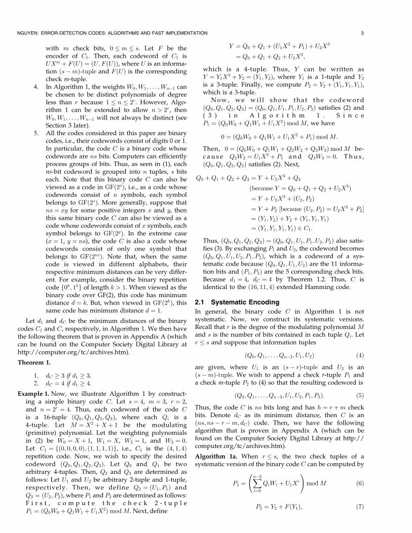
Example 2. Recall that C is an ðns; ns� r�m; dCÞ code thatis constructed by either Algorithm 1a (if r � s) orAlgorithm 1b (if r > s). This code has h ¼ rþm checkbits. In this example, we assume that h ¼ 16 bits and wepresent different ways to construct the codes C. Theresults are shown in Fig. 2. For example, usingAlgorithm 1b, we can construct the code C with thefollowing parameters: s ¼ 8, r ¼ 12, m ¼ 4, C1 ¼ ð8; 4; 4Þcode, a ¼ 1, and b ¼ 4 (a and b are not needed inAlgorithm 1a). Assume that the number of s-tuplessatisfies n � 2r, i.e., the number of bits in each codeword

4 IEEE TRANSACTIONS ON COMPUTERS, VOL. 54, NO. 1, JANUARY 2005

Fig. 2. Construction of the codes C using16 check bits.

is ns � 2rs ¼ 215. Then, the weighting polynomials Wi

can be chosen to be distinct. From Remark 2.1, we haved1 � 4. Then, from Theorem 1.2, all the codes C in Fig. 2have minimum distance dC ¼ 4.

3 SOME SPECIAL ERROR-DETECTION CODES

This section shows that the binary code C of Algorithm 1 isgeneral in the sense that it includes all the codes in Fig. 1 andother codes as special cases. Recall that Algorithm 1’ssystematic version is either Algorithm 1a (if r � s) orAlgorithm 1b (if r > s), where r is the degree of themodulating polynomial M and s is the number of bitscontained in each tuple Qi. The code C depends on thecomponents such as the parameters r;m; s; n, the weightsW0;W1; . . . ;Wn�1, and the code C1. Thus, different compo-nents will produce different codes C. We now show thatAlgorithm 1 produces the codes in Fig. 1 by letting C1 betrivial codes suchas ðs; s; 1) andf0sgdefined inRemark2.Thealgorithm also produces other linear and nonlinear codes(Sections 3.1, 3.6, and 3.8). Generally, codes of dC ¼ 4 requirethat n � 2r and the weightsW0;W1; . . . ;Wn�1 in Algorithm 1be distinct. Codes of dC ¼ 3 require that n � 2r þ 1 and allowsomeof theweights to be repeated.CodesofdC ¼ 2 also allowsome of the weights to be repeated, but do not restrict on thevalue of n, i.e., the code lengths can be arbitrary. Thefollowing codes are briefly presented because their detaileddiscussions can be found elsewhere [4], [5], [9], [14].

3.1 Binary Extended Perfect Code

We now show that Algorithm 1 produces an extendedperfect code if the code C1 is an extended perfect code.Suppose that C1 is a ð2m�1; 2m�1 �m; 4Þ extended perfectcode (see [8, Chapter 6]), i.e., s ¼ 2m�1 and d1 ¼ 4. Let n ¼ 2r

and h ¼ rþm, then the code C has ns ¼ 2rþm�1 ¼ 2h�1 bits.Then, dC ¼ 4 by Theorem 1.2 and C is a ð2h�1; 2h�1 � h; 4Þextended perfect code. Note that deleting a check bit froman extended perfect code will yield a perfect code, whileadding an overall even parity bit to a perfect code will yieldan extended perfect code.

Algorithms 1a and 1b can be further generalized toinclude the extended perfect code of [15] as follows: Recallthat P1, P2, and Y1 are the check r-tuple, check m-tuple, andðs�mÞ-tuple, respectively, which are computed fromAlgorithms 1a or 1b. Let Eð:Þ be any function from the setof ðs�mÞ-tuples to the set of r-tuples. Now, define the newcheck r-tuple and check m-tuple by

P �1 ¼ P1 þEðY1Þ and P �

2 ¼ P2 þ even parity of EðY1Þ:

Then, it can be shown that, if C1 is an extended perfect codeand n ¼ 2r, then the resulting code C whose check tuplesare P �

1 and P �2 is also an extended perfect code. Further,

when r ¼ 1, this extended perfect code becomes theextended perfect code that is obtained from the systematicperfect code of [15].

3.2 Weighted Sum Code (WSC)

Consider the code C for the special case s ¼ r ¼ m. ByRemark 2.1, we have C1 ¼ f0sg, U1 ¼ 0, U2 ¼ 0, Y1 ¼ 0, andY2 ¼ Y ¼

Pn�3i¼0 Qi þ P1. From (6) and (7) of Algorithm 1a,

we have

P1 ¼Xn�3

i¼0

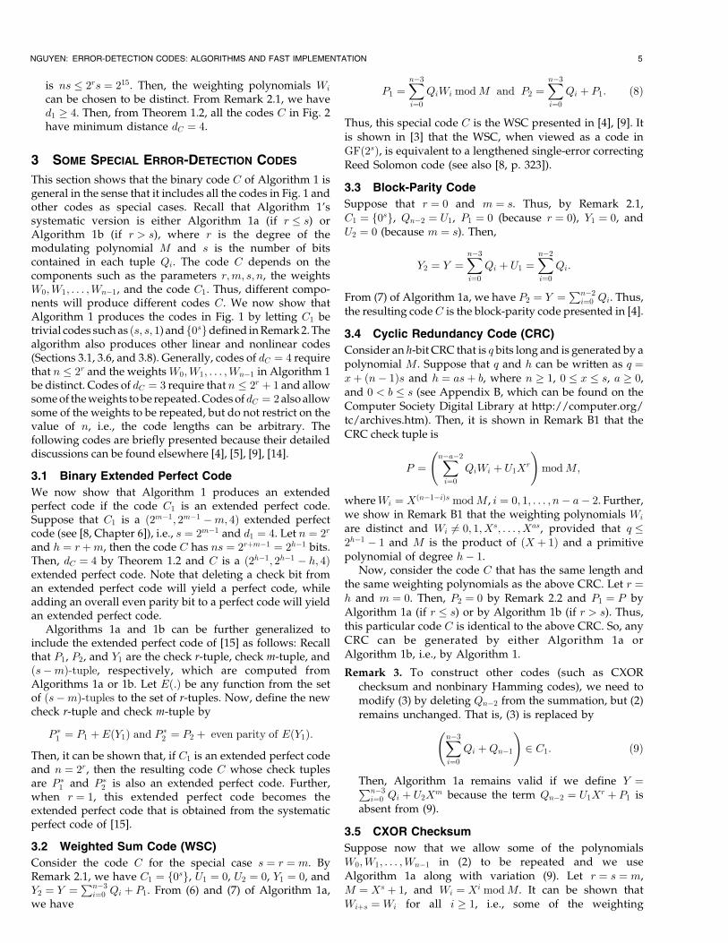
QiWi modM and P2 ¼Xn�3

i¼0

Qi þ P1: ð8Þ

Thus, this special code C is the WSC presented in [4], [9]. Itis shown in [3] that the WSC, when viewed as a code inGFð2sÞ, is equivalent to a lengthened single-error correctingReed Solomon code (see also [8, p. 323]).

3.3 Block-Parity Code

Suppose that r ¼ 0 and m ¼ s. Thus, by Remark 2.1,C1 ¼ f0sg, Qn�2 ¼ U1, P1 ¼ 0 (because r ¼ 0), Y1 ¼ 0, andU2 ¼ 0 (because m ¼ s). Then,

Y2 ¼ Y ¼Xn�3

i¼0

Qi þ U1 ¼Xn�2

i¼0

Qi:

From (7) of Algorithm 1a, we have P2 ¼ Y ¼Pn�2

i¼0 Qi. Thus,the resulting code C is the block-parity code presented in [4].

3.4 Cyclic Redundancy Code (CRC)

Consider an h-bit CRC that is q bits long and is generated by apolynomial M. Suppose that q and h can be written as q ¼xþ ðn� 1Þs and h ¼ asþ b, where n � 1, 0 � x � s, a � 0,and 0 < b � s (see Appendix B, which can be found on theComputer Society Digital Library at http://computer.org/tc/archives.htm). Then, it is shown in Remark B1 that theCRC check tuple is

P ¼Xn�a�2

i¼0

QiWi þ U1Xr

!modM;

whereWi ¼ Xðn�1�iÞs modM, i ¼ 0; 1; . . . ; n� a� 2. Further,we show in Remark B1 that the weighting polynomials Wi

are distinct and Wi 6¼ 0; 1; Xs; . . . ; Xas, provided that q �2h�1 � 1 and M is the product of ðX þ 1Þ and a primitivepolynomial of degree h� 1.

Now, consider the code C that has the same length andthe same weighting polynomials as the above CRC. Let r ¼h and m ¼ 0. Then, P2 ¼ 0 by Remark 2.2 and P1 ¼ P byAlgorithm 1a (if r � s) or by Algorithm 1b (if r > s). Thus,this particular code C is identical to the above CRC. So, anyCRC can be generated by either Algorithm 1a orAlgorithm 1b, i.e., by Algorithm 1.

Remark 3. To construct other codes (such as CXORchecksum and nonbinary Hamming codes), we need tomodify (3) by deleting Qn�2 from the summation, but (2)remains unchanged. That is, (3) is replaced by

Xn�3

i¼0

Qi þQn�1

!2 C1: ð9Þ

Then, Algorithm 1a remains valid if we define Y ¼Pn�3i¼0 Qi þ U2X

m because the term Qn�2 ¼ U1Xr þ P1 is

absent from (9).

3.5 CXOR Checksum

Suppose now that we allow some of the polynomialsW0;W1; . . . ;Wn�1 in (2) to be repeated and we useAlgorithm 1a along with variation (9). Let r ¼ s ¼ m,M ¼ Xs þ 1, and Wi ¼ Xi modM. It can be shown thatWiþs ¼ Wi for all i � 1, i.e., some of the weighting

NGUYEN: ERROR-DETECTION CODES: ALGORITHMS AND FAST IMPLEMENTATION 5

polynomials may repeat. Then, C1 ¼ f0sg (because m ¼ s),U1 ¼ 0 (because r ¼ s), and U2 ¼ Y1 ¼ 0 (because m ¼ s).From (6) and (7), we have P1 ¼

Pn�3i¼0 QiX

i mod ðXs þ 1Þand P2 ¼ Y2 ¼ Y ¼

Pn�3i¼0 Qi (see Remark 2.1 and

Remark 3). Thus, the resulting code C is the CXORchecksum presented in [4].

3.6 Nonbinary Perfect Code

Suppose that Algorithm 1a along with variation (9) isapplied with r ¼ s ¼ m and n ¼ 2m þ 1. Let M be aprimitive polynomial of degree m and let

W0;W1; . . . ;Wn�3

be distinct and nonzero polynomials. Then, C1 ¼ f0sg,P1 ¼

P2m�2i¼0 QiWi modM, and P2 ¼

P2m�2i¼0 Qi. It then can

be shown that P1 and P2 are two check tuples of thenonbinary Hamming perfect code over GFð2mÞ (see [8,Chapter 6]), i.e., the tuples ðQ0; Q1; . . . ; Q2m�2; P1; P2Þ formthe codewords of the Hamming perfect code over GFð2mÞ.

3.7 One’s-Complement Checksum and FletcherChecksum

The above codes are constructed using polynomial arith-metic because each tuple is considered as a polynomial overthe binary field f0; 1g. An alternative is to consider eachtuple as an integer and to use the rules of (one’s-complement) integer arithmetic to manipulate the codeconstruction. If we apply the integer arithmetic to theconstruction of the block-parity code and to the nonbinaryperfect code, we will get the one’s-complement checksumand Fletcher checksum, respectively. However, theseinteger-based codes are often weaker than their binarypolynomial counterparts (see Fig. 1). See [4], [5], [9] fordefinitions and performance comparisons of error-detectioncodes, including the one’s-complement and Fletcher check-sums. Thus, the integer-arithmetic version of Algorithm 1a,along with variation (9), also produces the one’s-comple-ment and Fletcher checksums. We will not discuss thesechecksums and integer-based codes any further becausethey are often weaker than their polynomial counterpartsand their analyses can be found elsewhere (e.g., [5], [14]).

3.8 Other Error-Detection Codes

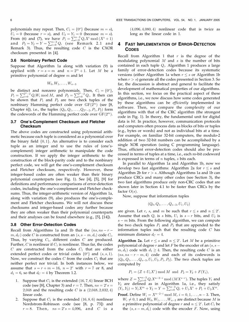
Recall from Algorithms 1a and 1b that the ðns; ns� r�m; dCÞ code C is constructed from an ðs; s�m; d1Þ code C1.Thus, by varying C1, different codes C are produced.Further, C is nonlinear if C1 is nonlinear. Thus far, the codesC are constructed from the codes C1 that are eitherextended perfect codes or trivial codes f0sg and ðs; s; 1Þ.Now, we construct the codes C from the codes C1 that areneither perfect nor trivial. In both instances below, weassume that s ¼ rþm ¼ 16, n ¼ 2r with r ¼ 7 or 8, andd1 ¼ 6, so that dC ¼ 4 by Theorem 1.2.

1. Suppose that C1 is the extended ð16; 7; 6Þ linear BCHcode (see [8], Chapter 3) and r ¼ 7. Then, ns ¼ 2rs ¼2;048 and the resulting code C is a ð2;048; 2;032; 4Þlinear code.

2. Suppose that C1 is the extended ð16; 8; 6Þ nonlinearNordstrom-Robinson code (see [8, p. 73]) andr ¼ 8. Then , ns ¼ 2rs ¼ 4;096, and C i s a

ð4;096; 4;080; 4Þ nonlinear code that is twice aslong as the linear code in 1.

4 FAST IMPLEMENTATION OF ERROR-DETECTION

CODES

Recall from Algorithm 1 that r is the degree of themodulating polynomial M and s is the number of bitscontained in each tuple Qi. Algorithm 1 produces a largefamily of error-detection codes because its systematicversions (either Algorithm 1a when r � s or Algorithm 1bwhen r > s) generate all the codes presented in Section 3. Sofar, the discussion is abstract and general to facilitate thedevelopment of mathematical properties of our algorithms.In this section, we focus on the practical aspect of thesealgorithms, i.e., we now discuss how some codes generatedby these algorithms can be efficiently implemented insoftware. Then, we compare the complexity of ouralgorithms with that of the CRC algorithm (the strongestcode in Fig. 1). In theory, the fundamental unit for digitaldata is bit. In practice, however, communication protocolsand computers often process data as blocks of bits or tuples(e.g., bytes or words) and not as individual bits at a time.For example, on familiar 32-bit computers, the modulo-2addition of two 32-bit numbers can be accomplished by asingle XOR operation (using C programming language).Thus, efficient error-detection codes should also be pro-cessed in terms of tuples at a time, i.e., each ns-bit codewordis expressed in terms of n tuples, s bits each.

In parallel to Algorithm 1a and Algorithm 1b, now wedevelop two fast algorithms: Algorithm 2a for r � s andAlgorithm 2b for r > s. Although Algorithms 1a and 1b canproduce CRCs and many other codes (see Section 3), thetwo fast algorithms produce only non-CRC codes that areshown later in Section 4.1 to be faster than CRCs by thefactor OðsÞ.

Now, suppose that information tuples

ðQ0; Q1; . . . ; Qn�3; U1; U2Þ

are given. Let r, s, and m be such that r � s and n � 2r.Assume that each Qi is s bits, U1 is s� r bits, and U2 iss�m bits. From the following algorithm, we can computethe two check tuples P1 and P2 that are appended to theinformation tuples such that the resulting code C hasminimum distance dC ¼ 4.

Algorithm 2a. Let r � s and n � 2r. Let M be a primitivepolynomial of degree r and let F be the encoder of an ðs; s�m; d1Þ code with d1 � 4. Then, the resulting code C is anðns; ns� r�m; 4Þ code and each of its codewords isðQ0; Q1; . . . ; Qn�3; U1; U2; P1; P2Þ. The two check tuples arecomputed by

P1 ¼ ðZ þ U1XrÞmodM and P2 ¼ Y2 þ F ðY1Þ;

where Z ¼Pn�3

i¼0 QiXn�2�i mod ðMXs�rÞ. The tuples Y1 and

Y2 are defined as in Algorithm 1a, i.e., they satisfyðY1; Y2Þ ¼ Y1X

m þ Y2 ¼ Y ¼Pn�3

i¼0 Qi þ U1Xr þ P1 þ U2X

m.

Proof. Define Wi ¼ Xn�2�i modM, i ¼ 0; 1; . . . ; n� 3. Then,Wi 6¼ 0; 1 and W0;W1; . . . ;Wn�3 are distinct because M isa primitive polynomial of degree r and n � 2r. Let C1 bethe ðs; s�m; d1Þ code with the encoder F . Now, using

6 IEEE TRANSACTIONS ON COMPUTERS, VOL. 54, NO. 1, JANUARY 2005

these Wi and C1 in Algorithm 1a, we can construct thecode C whose two check tuples are given by

P1 ¼Xn�3

i¼0

QiWi þ U1Xr

!modM and P2 ¼ Y2 þ F ðY1Þ:

Because d1 � 4, dC ¼ 4 by Theorem 1.2. Next, the newform of P1 is derived as follows: First, note that

Xs�rWi ¼ ðXs�rXn�2�iÞmod ðMXs�rÞ: ð10Þ

Multiplying P1 by Xs�r, we have

P1Xs�r ¼

Xn�3

i¼0

QiWi þ U1Xr

!Xs�r mod ðMXs�rÞ: ð11Þ

From (10), (11), the definition of Z, and somemodular algebra manipulation, it can be shown thatP1X

s�r ¼ ðXs�rZ þ U1XrXs�rÞmod ðMXs�rÞ. Thus,

P1Xs�r ¼ ððZ þ U1X

rÞmodMÞXs�r: ð12Þ

From (12), we have P1 ¼ ðZ þ U1XrÞmodM. tu

Remark 4. Let I and J be two binary polynomials ofdegrees i and j, respectively. In general, it is rathertedious to compute I mod J . However, when i � j, thecomputation becomes easy and is accomplished inconstant time because

I mod J ¼ I if i < jI þ J if i ¼ j:

�

This simple fact is used to efficiently compute Z ¼Pn�3i¼0 QiX

n�2�i mod ðMXs�rÞ in Algorithm 2a, as follows:Using Horner’s rule, we have

Z ¼ ð. . . ððQ0XÞmodN þQ1ÞX modN þ . . .þQn�3ÞmodN;

where N ¼ MXs�r. Then, Z can be recursivelycomputed from the polynomials Ti defined by T0 ¼Q0 a nd Ti ¼ ðTi�1XÞmodN þQi, i ¼ 1; . . . ; n� 3.Because s ¼ degN � degðTi�1XÞ, each Ti is computedin constant time, i.e., with Oð1Þ complexity. Finally, wehave Z ¼ ðTn�3XÞmodN . Thus, Z has computationalcomplexity OðnÞ. Horner’s rule is also used to efficientlyencode the WSC [4], [9].

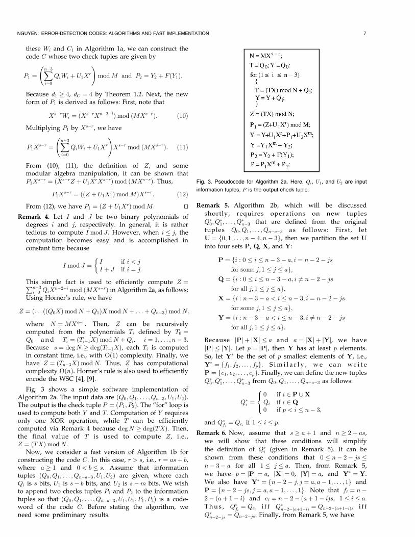
Fig. 3 shows a simple software implementation ofAlgorithm 2a. The input data are ðQ0; Q1; . . . ; Qn�3; U1; U2Þ.The output is the check tuple P ¼ ðP1; P2Þ. The “for” loop isused to compute both Y and T . Computation of Y requiresonly one XOR operation, while T can be efficientlycomputed via Remark 4 because degN � degðTXÞ. Then,the final value of T is used to compute Z, i.e.,Z ¼ ðTXÞmodN .

Now, we consider a fast version of Algorithm 1b forconstructing the code C. In this case, r > s, i.e., r ¼ asþ b,where a � 1 and 0 < b � s. Assume that informationtuples ðQ0; Q1; . . . ; Qn�a�3; U1; U2Þ are given, where eachQi is s bits, U1 is s� b bits, and U2 is s�m bits. We wishto append two checks tuples P1 and P2 to the informationtuples so that ðQ0; Q1; . . . ; Qn�a�3; U1; U2; P1; P2Þ is a code-word of the code C. Before stating the algorithm, weneed some preliminary results.

Remark 5. Algorithm 2b, which will be discussed

shortly, requires operations on new tuples

Q�0; Q

�1; . . . ; Q

�n�3 that are defined from the original

tuples Q0; Q1; . . . ; Qn�a�3 as follows: First, let

U ¼ f0; 1; . . . ; n� 4; n� 3g, then we partition the set U

into four sets P, Q, X, and Y:

P ¼ fi : 0 � i � n� 3� a; i ¼ n� 2� js

for some j; 1 � j � ag;Q ¼ fi : 0 � i � n� 3� a; i 6¼ n� 2� js

for all j; 1 � j � ag;X ¼ fi : n� 3� a < i � n� 3; i ¼ n� 2� js

for some j; 1 � j � ag;Y ¼ fi : n� 3� a < i � n� 3; i 6¼ n� 2� js

for all j; 1 � j � ag:

Because jPj þ jXj � a and a ¼ jXj þ jYj, we have

jPj � jYj. Let p ¼ jPj, then Y has at least p elements.

So, let Y� be the set of p smallest elements of Y, i.e.,

Y� ¼ ff1; f2; . . . ; fpg. S im i l a r l y , w e c a n w r i t e

P ¼ fe1; e2; . . . ; epg. Finally, we can define the new tuples

Q�0; Q

�1; . . . ; Q

�n�3 from Q0; Q1; . . . ; Qn�a�3 as follows:

Q�i ¼

0 if i 2 P [XQi if i 2 Q0 if p < i � n� 3;

8<:

and Q�fi¼ Qei if 1 � i � p.

Remark 6. Now, assume that s � aþ 1 and n � 2þ as,

we will show that these conditions will simplify

the definition of Q�i (given in Remark 5). It can be

shown from these conditions that 0 � n� 2� js �n� 3� a for all 1 � j � a. Then, from Remark 5,

we have p ¼ jPj ¼ a, jXj ¼ 0, jYj ¼ a, and Y� ¼ Y.

We also have Y� ¼ fn� 2� j; j ¼ a; a� 1; . . . ; 1g and

P ¼ fn� 2� js; j ¼ a; a� 1; . . . ; 1g. Note that fi ¼ n�2� ðaþ 1� iÞ and ei ¼ n� 2� ðaþ 1� iÞs, 1 � i � a.

Thus , Q�fi¼ Qei i f f Q�

n�2�ðaþ1�iÞ ¼ Qn�2�ðaþ1�iÞs i f f

Q�n�2�js ¼ Qn�2�js. Finally, from Remark 5, we have

NGUYEN: ERROR-DETECTION CODES: ALGORITHMS AND FAST IMPLEMENTATION 7

Fig. 3. Pseudocode for Algorithm 2a. Here, Qi, U1, and U2 are input

information tuples, P is the output check tuple.

Q�i ¼ Qi if i 6¼ n� 2� js; 1 � j � a; 0 � i � n� 3� a;

Q�n�2�js ¼ 0; 1 � j � a; and

Q�n�2�j ¼ Qn�2�js; 1 � j � a:

Basically, Q�0; Q

�1; . . . ; Q

�n�3 are obtained by moving

some a tuples of Q0; Q1; . . . ; Qn�a�3 to the right and

then by filling the a removed tuples by zeros. Now,

define Z ¼Pn�3

i¼0 Q�i X

n�2�i modM, which is a key

quantity in the following algorithm. This simplified

definition of Q�i makes it possible to calculate Z directly

from Qi (i.e., without using Q�i ). That is, we first modify

Qi using the following pseudocode:

forð1 � j � aÞQn�2�j ¼ Qn�2�js;

forð1 � j � aÞQn�2�js ¼ 0;

then we can compute Z directly from the modified Qi as

Z ¼Pn�3

i¼0 QiXn�2�i modM.

Now, we have the following algorithm that is proven in

Appendix A (which can be found on the Computer Society

Digital Library at http://computer.org/tc/archives.htm).

Algorithm 2b. Suppose that r > s and n � 2r. Let M be a

primitive polynomial of degree r and let F be the encoder of

an ðs; s�m; d1Þ code with d1 � 4. Then, the two check

tuples of the code C are computed by

P1 ¼ ðZ þ U1XrÞmodM and P2 ¼ Y2 þ F ðY1Þ;

where Z ¼Pn�3

i¼0 Q�i X

n�2�i modM and Q�i are defined in

Remark 5 (or in Remark 6 if applicable). The tuples Y1 and

Y2 are defined as in Algorithm 1b, i.e., they satisfy

ðY1; Y2Þ ¼ Y1Xm þ Y2 ¼ Y

¼Xn�a�3

i¼0

Qi

!þ U1X

b þ P10

� �þ

Xai¼1

P1i

!þ U2X

m;

where P10 is a b-tuple, and P11; . . . ; P1a are s-tuples that

satisfy P1 ¼ ðP10; P11; . . . ; P1aÞ. Further, C is an ðns; ns�r�m; 4Þ code.

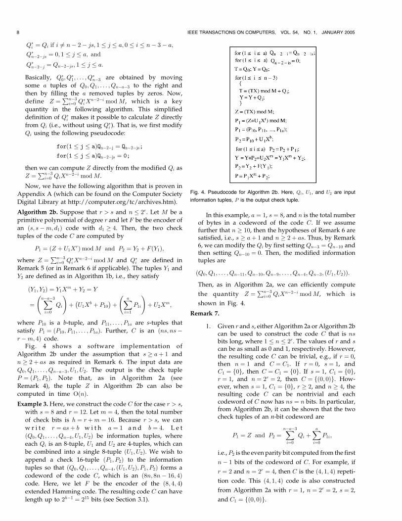
Fig. 4 shows a software implementation of

Algorithm 2b under the assumption that s � aþ 1 and

n � 2þ as as required in Remark 6. The input data are

Q0; Q1; . . . ; Qn�a�3; U1; U2. The output is the check tuple

P ¼ ðP1; P2Þ. Note that, as in Algorithm 2a (see

Remark 4), the tuple Z in Algorithm 2b can also be

computed in time OðnÞ.Example 3. Here, we construct the code C for the case r > s,

with s ¼ 8 and r ¼ 12. Let m ¼ 4, then the total number

of check bits is h ¼ rþm ¼ 16. Because r > s, we can

w r i t e r ¼ asþ b w i t h a ¼ 1 a n d b ¼ 4. L e t

ðQ0; Q1; . . . ; Qn�4; U1; U2Þ be information tuples, where

each Qi is an 8-tuple, U1 and U2 are 4-tuples, which can

be combined into a single 8-tuple ðU1; U2Þ. We wish to

append a check 16-tuple ðP1; P2Þ to the information

tuples so that ðQ0; Q1; . . . ; Qn�4; ðU1; U2Þ; P1; P2Þ forms a

codeword of the code C, which is an ð8n; 8n� 16; 4Þcode. Here, we let F be the encoder of the ð8; 4; 4)extended Hamming code. The resulting code C can have

length up to 2h�1 ¼ 215 bits (see Section 3.1).

In this example, a ¼ 1, s ¼ 8, and n is the total numberof bytes in a codeword of the code C. If we assumefurther that n � 10, then the hypotheses of Remark 6 aresatisfied, i.e., s � aþ 1 and n � 2þ as. Thus, by Remark6, we can modify the Qi by first setting Qn�3 ¼ Qn�10 andthen setting Qn�10 ¼ 0. Then, the modified informationtuples are

ðQ0; Q1; . . . ; Qn�11; Qn�10; Qn�9; . . . ; Qn�4; Qn�3; ðU1; U2ÞÞ:

Then, as in Algorithm 2a, we can efficiently compute

the quantity Z ¼Pn�3

i¼0 QiXn�2�i modM, which is

shown in Fig. 4.

Remark 7.

1. Given r and s, either Algorithm 2a or Algorithm 2bcan be used to construct the code C that is nsbits long, where 1 � n � 2r. The values of r and scan be as small as 0 and 1, respectively. However,the resulting code C can be trivial, e.g., if r ¼ 0,then n ¼ 1 and C ¼ C1. If r ¼ 0, s ¼ 1, andC1 ¼ f0g, then C ¼ C1 ¼ f0g. If s ¼ 1, C1 ¼ f0g,r ¼ 1, and n ¼ 2r ¼ 2, then C ¼ fð0; 0Þg. How-ever, when s ¼ 1, C1 ¼ f0g, r � 2, and n � 4, theresulting code C can be nontrivial and eachcodeword of C now has ns ¼ n bits. In particular,from Algorithm 2b, it can be shown that the twocheck tuples of an n-bit codeword are

P1 ¼ Z and P2 ¼Xn�a�3

i¼0

Qi þXai¼0

P1i;

i.e.,P2 is the even parity bit computed from the first

n� 1 bits of the codeword of C. For example, if

r ¼ 2 and n ¼ 2r ¼ 4, then C is the ð4; 1; 4Þ repeti-tion code. This ð4; 1; 4Þ code is also constructed

from Algorithm 2a with r ¼ 1, n ¼ 2r ¼ 2, s ¼ 2,

and C1 ¼ fð0; 0Þg.

8 IEEE TRANSACTIONS ON COMPUTERS, VOL. 54, NO. 1, JANUARY 2005

Fig. 4. Pseudocode for Algorithm 2b. Here, Qi, U1, and U2 are input

information tuples, P is the output check tuple.

2. Let r ¼ 1, then M ¼ X þ 1. Thus, the code C is2s b i t s l o n g ( b y A l g o r i t hm 2a ) a ndP1 ¼ ðU1XÞmod ðX þ 1Þ, which is the even parityof U1. For example, let C1 be the ð4; 1; 4Þ code, thenwe can construct the code C of length 8, which isthe ð8; 4; 4Þ extended Hamming code. If we setC1 ¼ ð8; 4; 4Þ code, then we can construct the codeC of length 16, i.e., C ¼ ð16; 11; 4Þ code. Repeatingthis process, we can construct ð32; 26; 4Þ andð64; 57; 4Þ codes. This method is related to thescheme of [15] and is effective to construct codesthat are small enough to fit into the computerwords.

3. Let r � 0, s � 1, C1 ¼ ðs; s�m; d1Þ with d1 � 4,and h ¼ rþm. Then, using either Algorithm 2a(if r � s) or Algorithm 2b (if r > s), we canconstruct the code C that is an ðns; ns� h; 4Þcode. In particular, if n ¼ 2r, then C is a ð2rs; 2rs�h; 4Þ code. That is, starting from a code C1 oflength s, we can construct the code C of length2rs. Further, if C1 is a ð2m�1; 2m�1 �m; 4Þ ex-tended perfect code, then C is a ð2h�1; 2h�1 � h; 4Þextended perfect code. If C1 is a linear perfectcode, then C is also a linear perfect code. Thislinear perfect code C and the extended Hammingperfect code of length 2h�1 are equivalent, i.e., onecode can be obtained from the other code byreordering the bit positions and adding a constantvector (see [8, p. 39]). Equivalent codes have thesame minimum distance and length, but theirimplementation complexity can be very different.However, our algorithms can also generate fastcodes that are different from the perfect codes.For example, in Algorithm 2a, let s ¼ 16 and let Fbe the encoder of the extended ð16; 8; 6Þ nonlinearNordstrom-Robinson code (see also Section 3.8).Then, the resulting code C is a nonlinear codewith dC ¼ 4, which is not equivalent to anyextended perfect codes.

4.1 Software Complexity

Now, we compare software complexity between the code C

and the CRC (the strongest code in Fig. 1). Here, we focus

on implementations that require no table lookup. Table-

lookup methods are discussed later in Remark 8.2Suppose that s � r. Then, the binary code C of length

ns bits can be constructed using Algorithm 2a whose

complexity is dominated by the computation of Z and Y ,

which can be computed by the for-loop in Fig. 3. Within this

for-loop, the expression T ¼ ðTXÞmodN þQi is computed

in constant time (by Remark 4), while the expression Y ¼Y þQi is computed by one XOR operation. Thus, this for-

loop has complexity OðnÞ. Hence, the time complexity of

the code C is also OðnÞ. Similarly, when s < r, the code C

under Algorithm 2b also has time complexity OðnÞ (see

Fig. 4). In summary, regardless of s � r or s < r, the code C

of length ns can be encoded with time complexity OðnÞ.Now, consider the CRC that also has length ns bits. Here,

we limit our discussions to a generic CRC algorithm, i.e., a

general algorithm that is applicable to all generating

polynomials. Then, it is shown in Remark B3(a) that thegeneric CRC algorithm has time complexity OðnsÞ. Forsome specific generating polynomials whose nonzero termssatisfy certain desirable properties, alternative algorithms(such as shift and add [4] and on-the-fly [11]) may havelower complexity.

When s is considered as a constant, we haveOðnsÞ ¼ OðnÞ. Thus, from a purely theoretical viewpoint,both the CRC and the code C have the same level ofcomplexity. However, the extra factor s does not appear inthe time complexity of the code C, i.e., the code C isapproximately faster than the CRC by the factor OðsÞ. Wewill show later, in Remark 8.1, that OðsÞ � 0:73s when theseerror-detection codes are implemented in C programminglanguage.

Example 4. Here, we study codes of h ¼ 16 check bits (othervalues of h are discussed later in Remark 8.1). Assumethat C1 is the ðs; s�m; 4Þ extended Hamming code andthe resulting code C is constructed by Algorithm 2a orAlgorithm 2b. Thus, both the CRC and the code C haveminimum distance d ¼ 4 and the maximum code lengthsof the code C and of the CRC are 215 and 215 � 1 � 215

bits, respectively (see also Remark 7.3). Thus, in terms ofthe minimum distance and maximum code length, thecode C and the CRC perform almost identically. Ourgoal here is to compare the software complexity of thesetwo codes. Software complexity refers to the number ofsoftware operations to process one byte of a codeword.Here, a code is called “faster” if it has lower operationcount. Simply stated, we write software programs (inC programming language) for the code C and the CRC.Then, we count the number of software operationsneeded by each code to encode one byte of a codeword.Computer programs for these codes and the rules forcounting the operations are given in Appendix D (whichcan be found on the Computer Society Digital Library athttp://computer.org/tc/archives.htm).

Recall that a typical codeword consists of n tuples,each tuple has s bits. Let tCðs; nÞ and tCRCðs; nÞ be thesoftware operation count required to compute the h ¼ 16check bits for a codeword of the code C and of the CRC,respectively. Then, from (29) of Appendix D (which canbe found on the Computer Society Digital Library athttp://computer.org/tc/archives.htm), we have

tCðs; nÞ ¼ 7:5nþ fðsÞ;

where fð8Þ ¼ 33:5, fð16Þ ¼ 51, fð32Þ ¼ 165:5, andfð64Þ ¼ 372. From Algorithms 2a and 2b, the two checktuples are given by P1 ¼ ðZ þ U1X

rÞmodM andP2 ¼ Y2 þ F ðY1Þ. The first component of tCðs; nÞ is 7:5nand represents the cost of computing Z and Y ¼ ðY1; Y2Þ,while the second component fðsÞ is the cost of comput-ing ðZ þ U1X

rÞmodM and Y2 þ F ðY1Þ. The first compo-nent varies as a linear function of the tuple count n, whilethe second component fðsÞ depends only on the tuplesize s and not on n. Thus, fðsÞ is a transient componentwhose contribution becomes negligible for large n.

For the CRC, from (30) of Appendix D (which can befound on the Computer Society Digital Library at http://computer.org/tc/archives.htm), we have

NGUYEN: ERROR-DETECTION CODES: ALGORITHMS AND FAST IMPLEMENTATION 9

tCRCðs; nÞ ¼ 5:5nsþ 3n� gðsÞ;

where gð8Þ ¼ 52, gð16Þ ¼ 93, gð32Þ ¼ gð64Þ ¼ 90. For

example, let s ¼ 8 and n ¼ 64, i.e., ns ¼ 29 ¼ 512 bits.

Then, tCð8; 64Þ ¼ ð7:5Þð64Þ þ 33:5 ¼ 513:5, i.e., the code C

needs 513.5 operations to process 512 bits. Thus, the

operat ion count per byte of the code C is

ð8Þð513:5Þ=512 ¼ 8:02. Similarly, it can be shown that

the operation count per byte of the CRC is 46.2. Then, the

ratio of the byte operation counts of the CRC and the

code C is 46:2=8:02 ¼ 5:76, i.e., the code C is 5.76 times

faster than the CRC. The triplet ð46:2; 8:02; 5:76Þ for the

pair ðs; nsÞ ¼ ð8; 29Þ is recorded in the left top part of

Fig. 5. Triplets for other pairs ðs; nsÞ are similarly

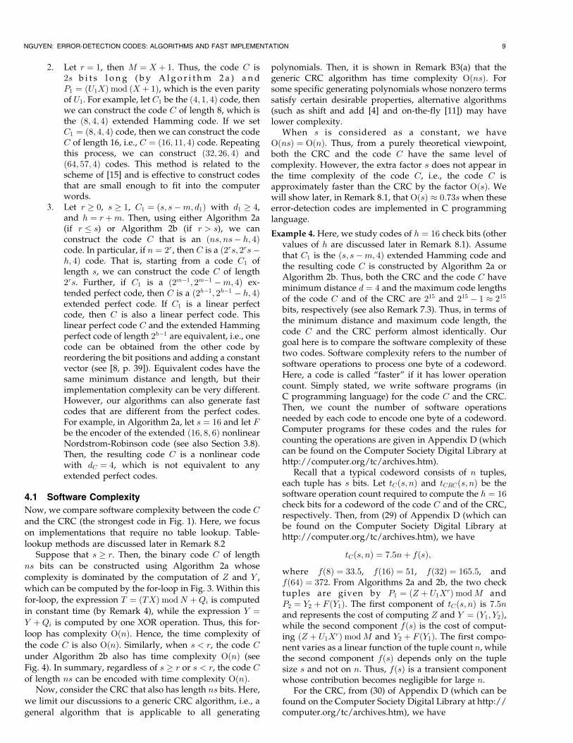
obtained.The results for software complexity of these two codes

are summarized in Fig. 5, where n is the total number ofs-tuples in a codeword, i.e., the total codeword length isns bits. Here, we consider a wide range of codewordlengths: from 29 to 215 bits (i.e., from 64 to 4,096 bytes).Each cell has three numbers: The first number is theoperation count per byte of the CRC, the second numberis the operation count per byte of the code C, the thirdnumber is the ratio of the above two numbers andrepresents the speed improvement of the code Ccompared to the CRC.

From Fig. 5, as expected, the byte operation count of

the CRC slightly decreases when s increases because

processing of larger tuples reduces loop overhead. The

CRC’s operation count also slightly decreases with

decreasing n due to the negative term �gðs) in

tCRCðs; nÞ. Note that the operation count of the CRC

varies only slightly over a wide range of the tuple size s

and of the codeword length ns. In contrast, the operation

count of the code C varies much more as a function of s

and ns. Further, for each tuple size s, the code C is faster

for longer codeword length ns. This is desirable because

speed is more important for longer messages. The reason

for the speed variation of the code C is the contribution

from the transient term fðsÞ to the code overall speed.

This contribution is noticeable (negligible) if the code-

words are short (long). For smaller tuple size s (such as

s ¼ 8 and 16), the transient term is smaller. Thus, the

overall speed variation (as a function of ns) of the code C

is also smaller. For larger s (such as s ¼ 32 and 64), the

transient term is greater, resulting in more speed

variation (as a function of ns) for the code C. From

Fig. 5, the code C is substantially faster than the CRC,

especially for the tuple size s ¼ 32 or 64 bits and the code

length ns � 213 bits ¼ 1;024 bytes. In particular, if the

code length is ns ¼ 215 bits ¼ 4;096 bytes, then the code

C is 23.4 and 43.1 times faster than the CRC when s is 32

and 64 bits, respectively.

Remark 8.

1. In Example 4, we derive the operation countexpressions tCðs; nÞ and tCRCðs; nÞ for the specialcase h ¼ 16 check bits (when the codes areimplemented in C programming language).There, we also assume that the code C1 used inthe construction of the code C is the extendedHamming code of length s. No such C1 code isneeded for the CRC. However, from Figs. 3 and 4,the same expressions also hold true for othervalues of h and for other codes C1, but withdifferent transient terms that are now denoted asfðs; h; C1Þ and gðs; hÞ to reflect the their depen-dency on s, h, and C1. Thus, in general, thesoftware operation counts required to computethe h check bits for a codeword (which consists ofn tuples, each tuple is s bits) of these two codesare:

tCðs; n; h; C1Þ ¼ 7:5nþ fðs; h; C1ÞtCRCðs; n; hÞ ¼ 5:5nsþ 3n� gðs; hÞ;

where the transient terms fðs; h; C1Þ and gðs; hÞare independent of n and their contributionsbecome negligible when n is large enough. Thus,for large n, we have

tCRCðs; n; hÞtCðs; n; h; C1Þ

� 5:5nsþ 3n

7:5n� 5:5ns

7:5n¼ 0:73s;

which is an estimate of the speed improvement ofthe code C compared to the CRC. Again, for largen, the code C needs approximately 7.5 operationsto process one s-tuple or 60=s operations per byte.Recall that, in general, the code C is faster thanthe CRC by the factor OðsÞ. Thus, we have OðsÞ �0:73s when these error-detection codes are im-plemented in C programming language.

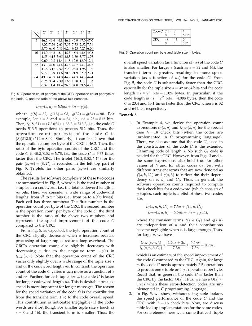
2. In Fig. 5, we show, without using table lookup,the speed performance of the code C and theCRC, with h ¼ 16 check bits. Now, we discusstable-lookup implementations for the same codes.For concreteness, here we assume that each tuple

10 IEEE TRANSACTIONS ON COMPUTERS, VOL. 54, NO. 1, JANUARY 2005

Fig. 5. Operation count per byte of the CRC, operation count per byte of

the code C, and the ratio of the above two numbers.

Fig. 6. Operation count per byte and table size in bytes.

Qi has size s ¼ 8 bits, as is often used in table-lookup implementations of common CRCs. Lar-ger values of s can be similarly handled, but theyresult in much larger table sizes. The results areshown in Fig. 6 (whose detailed derivation isgiven in Appendix D.1, which can be found onthe Computer Society Digital Library at http://computer.org/tc/archives.htm). Note that, be-cause s ¼ 8 is a small value, the transient termsfðs; h; C1Þ and gðs; hÞ are also small compared tothe code overall operation counts. Thus, weestimate the overall operation counts by omittingthese transient terms. In particular, the secondcolumn shows that, without using table lookup,the code C and the CRC use 7.5 and 47 operationsper byte, respectively. The exact values, whichvary from 7.51 to 8.02 (for the code C) and from46.2 to 47 (for the CRC), are recorded in Fig. 5.The estimated operation counts and table sizesare shown in Fig. 6. As expected, the operationcounts become smaller at the cost of larger tables.

5 SUMMARY AND CONCLUSIONS

We develop Algorithm 1 for generating a large and generalfamily of binary error-detection codes. This algorithm hastwo key parameters, s and r, where s is the size of eachtuple and r is the degree of the modulating polynomial M.Algorithm 1 is expressed in general and abstract form tofacilitate the mathematical development of the resultingcode C. Error-detection codes used in practice are oftensystematic. Thus, Algorithm 1 is transformed into systema-tic versions to yield Algorithm 1a (if r � s) and Algorithm 1b(if r > s).

A variety of error-detection codes (such as CRCs,checksums, and other codes listed in Fig. 1) are developedover the years for applications that require reliablecommunication or storage. These codes are traditionallyconsidered as unrelated and independent of each other.They also differ considerably in performance and complex-ity. More complex codes such as CRCs are stronger codes(with minimum distance d ¼ 4), whereas simple checksumssuch as block-parity codes are weaker codes (with d ¼ 2). InSection 3, we show that all these diverse codes (from CRCsto checksums), as well as other linear and nonlinear codes,are special cases of Algorithm 1. Thus, these seeminglyunrelated codes, which are independently developed overmany years, come from a single algorithm.

From Fig. 1, CRCs have the best error-detection cap-ability, but introduce the longest encoding delay. In thispaper, we then introduce some non-CRC codes that havegood error-detection capabilities as well as fast encoding. InSection 4, we present Algorithm 2a (for r � s) andAlgorithm 2b (for r > s), which are fast versions ofAlgorithm 1a and Algorithm 1b, respectively. These twofast algorithms produce only non-CRC codes. Further, someof these non-CRC codes are not only fast but also reliable.To achieve the minimum distance ¼ 4 using h check bits,CRC length can be up to 2h�1 � 1 bits, while the length ofsome non-CRC codes can be up to 2h�1 bits (i.e., they are

fast versions of perfect codes). We compare the computa-tional complexity of these CRCs and non-CRC codes usingmethods that require no table lookup. For long messages,the non-CRC codes can be faster than the CRCs by the factorOðsÞ. Further, OðsÞ � 0:73s when these codes are imple-mented in C programming language. Finally, with the useof table lookup, the operation counts are reduced at the costof precomputed tables.

ACKNOWLEDGMENTS

This work was supported in part by the US Office of NavalResearch.

REFERENCES

[1] D. Bertsekas and R. Gallager, Data Networks, second ed. Engle-wood Cliffs, N.J.: Prentice Hall, 1992.

[2] A. Binstock and J. Rex, Practical Algorithms for Programmers.Reading, Mass.: Addison-Wesley, 1995.

[3] P. Farkas, “Comments on ’Weighted Sum Codes for ErrorDetection and Their Comparison with Existing Codes’,” IEEE/ACM Trans. Networking, vol. 3, no. 2, pp. 222-223, Apr. 1995.

[4] D.C. Feldmeier, “Fast Software Implementation of Error DetectionCodes,” IEEE/ACM Trans. Networking, vol. 3, no. 6, pp. 640-651,Dec. 1995.

[5] J.G. Fletcher, “An Arithmetic Checksum for Serial Transmissions,”IEEE Trans. Comm., vol. 30, pp. 247-252, Jan. 1982.

[6] J.G. Fletcher, ACM Computing Rev., vol. 36, no. 1, p. 66, Jan. 1995.[7] T. Klove and V. Korzhik, Error Detecting Codes: General Theory and

Their Application in Feedback Communication Systems. KluwerAcademic, 1995.

[8] F.J. MacWilliams and N.J. A. Sloan, The Theory of Error-CorrectingCodes. New York: North-Holland, 1977.

[9] A.J. McAuley, “Weighted Sum Codes for Error Detection andTheir Comparison with Existing Codes,” IEEE/ ACM Trans.Networking, vol. 2, no. 1, pp. 16-22, Feb. 1994.

[10] G.D. Nguyen, “A General Class of Error-Detection Codes,” Proc.32nd Conf. Information Sciences and Systems, pp. 451-453, Mar. 1998.

[11] A. Perez, “Byte-Wise CRC Calculations,” IEEEMicro, vol. 3, pp. 40-50, June 1983.

[12] T.V. Ramabadran and S.S. Gaitonde, “A Tutorial on CRCComputations,” IEEE Micro, vol. 8, pp. 62-75, Aug. 1988.

[13] D.V. Sarwate, “Computation of Cyclic Redundancy Checks viaTable-Lookup,” Comm. ACM, vol. 31, no. 8, pp. 1008-1013, Aug.1988.

[14] J. Stone, M. Greenwald, C. Partridge, and J. Hughes, “Performanceof Checksums and CRC’s over Real Data,” IEEE/ACM Trans.Networking, vol. 6, no. 5, pp. 529-543, Oct. 1998.

[15] J.L. Vasilev, “On Nongroup Close-Packed Codes (in Russian),”Problemi Cybernetica, vol. 8, pp. 337-339, 1962.

Gam D. Nguyen received the PhD in electricalengineering from the University of Maryland,College Park, in 1990. He has been at the USNaval Research Laboratory, Washington, DC,since 1991. His research interests includecommunication systems and networks.

. For more information on this or any other computing topic,please visit our Digital Library at www.computer.org/publications/dlib.

NGUYEN: ERROR-DETECTION CODES: ALGORITHMS AND FAST IMPLEMENTATION 11