ERROR CONTROL 343 Introduction 3.144 Error Model 3.2

46 Types of Transmission Errors 3.346 Redundancy 3.4

47 Types of Codes 3.548 Parity Check 3.6

48 Error Correction 3.752 A Linear Block Code 3.8

56 Cyclic Redundancy Checks 3.963 Arithmethic Checksum 3.10

64 Summary 3.1164 Exercises

65 Bibliographic Notes

3.1 INTRODUCTIONThe number of errors caused by data transmission is typically orders of magnitudelarger than the number of errors caused by hardware failures within a computer sys-tem. The bit error probability for internal circuits is usually below 10 − 15. On an opti-cal fiber link the average probability of errors is approximately 10 − 9. That is, on theaverage, one in every 109 bits transmitted (or processed) is distorted, six orders ofmagnitude more than for hardware circuits. Similarly, on a coaxial cable the proba-bility of bit errors is approximately 10 − 6. For a switched telephone line, the numbersare even higher, between 10 − 4 and 10 − 5.

The difference in magnitude between an error probability of 10 − 15 and one of 10 − 4

should not be underestimated. A bit error rate of 10 − 15 on a transmission line wouldbe immeasurably small at today’s transmission rates. At a rate of 9600 bits persecond, it would cause one single bit error every 3303 years of continuous operation.At the same data rate, a bit error rate of 10 − 4 causes a bit error, on average, once asecond.

Depending on line and network characteristics, transmitted data may be reordered,distorted, or deleted, and occasionally noisy lines may even insert new data intotransmissions. The errors introduced in data transmissions are, of course, not entirelyunpredictable or inexplicable. The errors have two main causes, discussed in moredetail in Appendix A:

Linear distortion of the original data, for instance, as caused by bandwidth lim-itations of the raw data channelNon-linear distortion that is caused by echoes, cross-talk, white noise, and

43

44 ERROR CONTROL CHAPTER 3

impulse noiseThe effect of these distortions can be remedied, to a certain extent, with cable insula-tion and hardware compensation filters. The errors that remain must be caught insoftware by the communications protocol.

There are several ways in which the error characteristics of a data line can beexpressed. The first, and most important, is the long-term average bit error rate. But,since this is only an average, there are two other factors in use:

The percentage of time that the average bit error rate does not exceed a giventhreshold valueThe percentage of error-free seconds

The last two measures give an indication of the overall quality of a line or a network.For the design of an error control method one commonly uses only the average biterror rate, as an indication of the expected performance.

No error control method can be expected to catch all errors that can possibly occur.We can, however, require that an error control scheme increase the reliability of thetransmissions, preferably to the level of reliability of the stand-alone operation of acomputer.

An often overlooked issue is that an effective error control scheme should match theerror characteristics of the channels to be used. If a channel only produces insertionerrors, it would be unwise to design a protocol that protects against deletions. Simi-larly, if a channel produces independent, single-bit errors with a relatively low proba-bility, even the simplest parity scheme (Section 3.6) can easily outperform the mostsophisticated error control methods. And, finally, if the error rate of the channel isalready lower than that of peripheral equipment, the inclusion of any error controlscheme needlessly degrades performance and may even turn out to decrease ratherthan increase the protocol’s reliability.

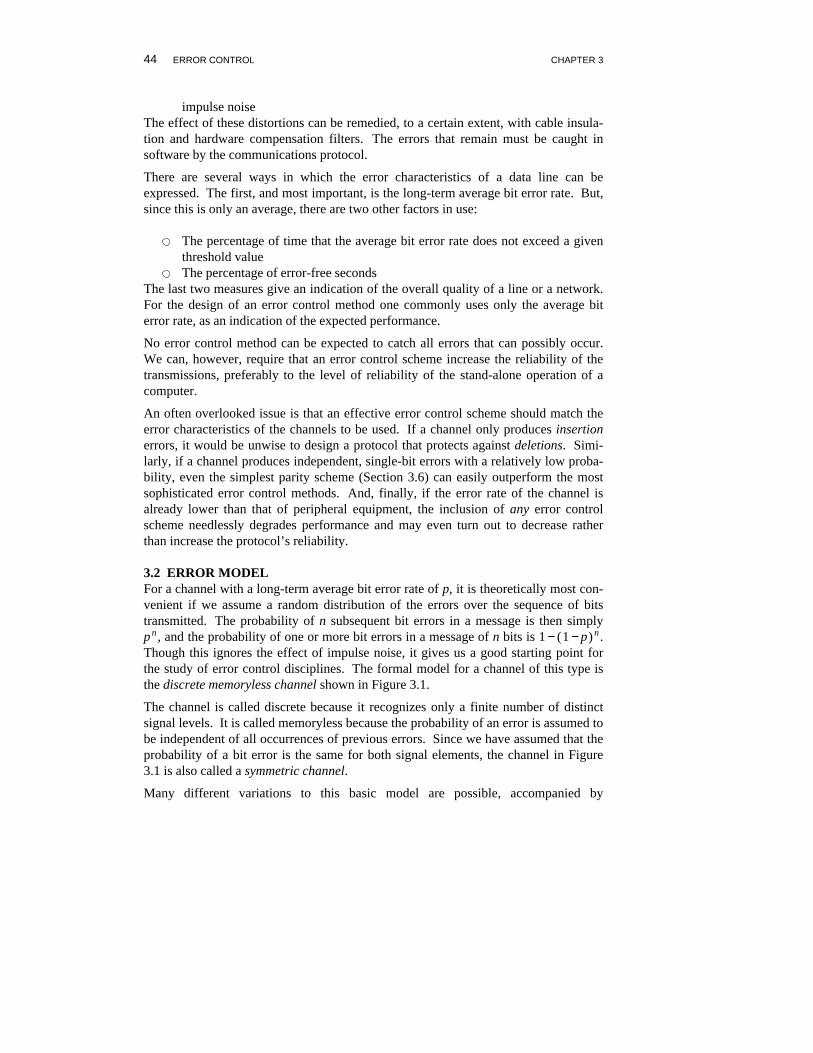
3.2 ERROR MODELFor a channel with a long-term average bit error rate of p, it is theoretically most con-venient if we assume a random distribution of the errors over the sequence of bitstransmitted. The probability of n subsequent bit errors in a message is then simplyp n , and the probability of one or more bit errors in a message of n bits is 1 − ( 1 − p) n .Though this ignores the effect of impulse noise, it gives us a good starting point forthe study of error control disciplines. The formal model for a channel of this type isthe discrete memoryless channel shown in Figure 3.1.

The channel is called discrete because it recognizes only a finite number of distinctsignal levels. It is called memoryless because the probability of an error is assumed tobe independent of all occurrences of previous errors. Since we have assumed that theprobability of a bit error is the same for both signal elements, the channel in Figure3.1 is also called a symmetric channel.

Many different variations to this basic model are possible, accompanied by

SECTION 3.2 ERROR MODEL 45

0

1

q = 1−p0

1q = 1−p

p

p

Figure 3.1 — Discrete Memoryless Channelincreasingly complex calculations to predict the effect of error control methods. In anasymmetric channel, for instance, the probability of an error may depend on the signalvalue being transmitted. The distribution of error probabilities can also be defined asa process with memory: if the last n bits transmitted were in error it is very probablethat the next few will be wrong too. It is difficult to capture this behavior in a predic-tive model. The error model provided by the binary symmetric channel predicts thatthe probability of a series of at least n contiguous error-free bit transmissions, calledan ‘‘error-free interval’’ (EFI), is equal to

Pr(EFI≥n) = ( 1 − b) n, n≥0 (3.1)

where b is the long-term average bit error rate.

The probability decreases linearly with the length of the interval. Similarly, the pro-bability that the duration of a burst exceeds n bits decreases linearly with n. Toexpress that the probability of an error-free interval decreases exponentially with itsduration, we can replace formula (3.1) with a Poisson distribution:

Pr(EFI≥n) = e− b(n − 1 ) , n ≥ 1 (3.2)

The best way to verify the accuracy of this prediction is, of course, to compare itagainst empirical data. Such studies indicate indeed that formula (3.2) predicts errorfree intervals better than (3.1). A still better match can be found if a correction factoris added to (3.2). We thus obtain the following approximation, which is due to BenoitMandelbrot (see Bibliographic Notes):

Pr(EFI≥n) = n ( 1 − a) − (n − 1 )( 1 − a)

e− b(n − 1 ) , 0≤a < 1 , n ≥ 1 (3.3)

The parameter a determines how serious the clustering effect is predicted to be.When a is zero, formula (3.3) reduces to the Poisson distribution in (3.2). For non-zero a, the probability of longer error-free intervals decreases more than the probabil-ity of shorter intervals. With growing a this effect becomes more pronounced. Ofcourse, if the error characteristics are independent of the bit rate they can be expressedin seconds.

With different parameter values a and b, functions of type (3.2) and (3.3) can be usedto predict both the duration of error-free intervals and the duration of bursts indepen-dently. We will use this method in Chapter 7. For the remainder of this chapter,however, we will restrict ourselves to the model of a binary symmetric channel.

46 ERROR CONTROL CHAPTER 3

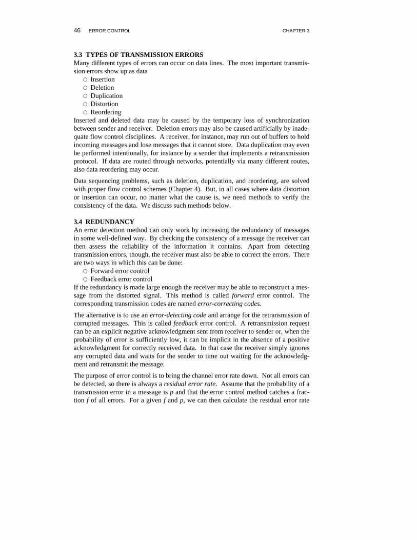
3.3 TYPES OF TRANSMISSION ERRORSMany different types of errors can occur on data lines. The most important transmis-sion errors show up as data

InsertionDeletionDuplicationDistortionReordering

Inserted and deleted data may be caused by the temporary loss of synchronizationbetween sender and receiver. Deletion errors may also be caused artificially by inade-quate flow control disciplines. A receiver, for instance, may run out of buffers to holdincoming messages and lose messages that it cannot store. Data duplication may evenbe performed intentionally, for instance by a sender that implements a retransmissionprotocol. If data are routed through networks, potentially via many different routes,also data reordering may occur.

Data sequencing problems, such as deletion, duplication, and reordering, are solvedwith proper flow control schemes (Chapter 4). But, in all cases where data distortionor insertion can occur, no matter what the cause is, we need methods to verify theconsistency of the data. We discuss such methods below.

3.4 REDUNDANCYAn error detection method can only work by increasing the redundancy of messagesin some well-defined way. By checking the consistency of a message the receiver canthen assess the reliability of the information it contains. Apart from detectingtransmission errors, though, the receiver must also be able to correct the errors. Thereare two ways in which this can be done:

Forward error controlFeedback error control

If the redundancy is made large enough the receiver may be able to reconstruct a mes-sage from the distorted signal. This method is called forward error control. Thecorresponding transmission codes are named error-correcting codes.

The alternative is to use an error-detecting code and arrange for the retransmission ofcorrupted messages. This is called feedback error control. A retransmission requestcan be an explicit negative acknowledgment sent from receiver to sender or, when theprobability of error is sufficiently low, it can be implicit in the absence of a positiveacknowledgment for correctly received data. In that case the receiver simply ignoresany corrupted data and waits for the sender to time out waiting for the acknowledg-ment and retransmit the message.

The purpose of error control is to bring the channel error rate down. Not all errors canbe detected, so there is always a residual error rate. Assume that the probability of atransmission error in a message is p and that the error control method catches a frac-tion f of all errors. For a given f and p, we can then calculate the residual error rate

SECTION 3.5 TYPES OF CODES 47

p .( 1 − f ) and convince ourselves that it is, for instance, in the order of 10− 9 or less.

If probability p is very close to zero, an error-correcting code is generally ill-advised:it merely slows down the data transfer. If, on the other hand, p approaches one, aretransmission scheme would be a bad choice: almost every message, including theretransmitted ones, would be hit. Of course there are exceptions to these rules. If p issmall, and the cost of retransmission high, a forward error control scheme may still beprofitable. In other cases still, a combination of forward and feedback error controlmay be a good compromise: the receiver corrects frequently occurring errors and asksthe sender for the retransmission of messages that contain less frequent errors.

In the next section we first look at the main types of error-correcting and error-detecting codes that have been developed.

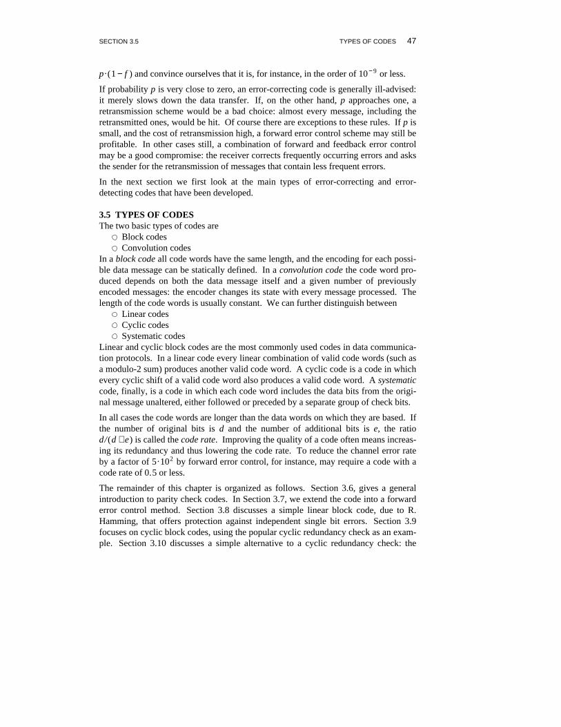
3.5 TYPES OF CODESThe two basic types of codes are

Block codesConvolution codes

In a block code all code words have the same length, and the encoding for each possi-ble data message can be statically defined. In a convolution code the code word pro-duced depends on both the data message itself and a given number of previouslyencoded messages: the encoder changes its state with every message processed. Thelength of the code words is usually constant. We can further distinguish between

Linear codesCyclic codesSystematic codes

Linear and cyclic block codes are the most commonly used codes in data communica-tion protocols. In a linear code every linear combination of valid code words (such asa modulo-2 sum) produces another valid code word. A cyclic code is a code in whichevery cyclic shift of a valid code word also produces a valid code word. A systematiccode, finally, is a code in which each code word includes the data bits from the origi-nal message unaltered, either followed or preceded by a separate group of check bits.

In all cases the code words are longer than the data words on which they are based. Ifthe number of original bits is d and the number of additional bits is e, the ratiod /(d + e) is called the code rate. Improving the quality of a code often means increas-ing its redundancy and thus lowering the code rate. To reduce the channel error rateby a factor of 5.102 by forward error control, for instance, may require a code with acode rate of 0. 5 or less.

The remainder of this chapter is organized as follows. Section 3.6, gives a generalintroduction to parity check codes. In Section 3.7, we extend the code into a forwarderror control method. Section 3.8 discusses a simple linear block code, due to R.Hamming, that offers protection against independent single bit errors. Section 3.9focuses on cyclic block codes, using the popular cyclic redundancy check as an exam-ple. Section 3.10 discusses a simple alternative to a cyclic redundancy check: the

48 ERROR CONTROL CHAPTER 3

arithmetic checksum method.

3.6 PARITY CHECKIf the probability of multiple bit errors per message is sufficiently low, all the errorcontrol needed on a binary symmetric channel is a parity check code. To every mes-sage we add a single bit that makes the modulo-2 sum of the bits in that messageequal to one. The overhead is merely one bit per message. If any single bit, includingthe check bit, is distorted by the channel the parity at the receiver comes out wrongand the transmission error can be detected.

If we set q = 1 − p, the probability of an error-free transmission of n message bits plusone parity bit is q (n + 1 ) , and the probability of a single bit error in n + 1 bits transmit-ted is the binomial probability (n + 1 ) .p .q n . Under these assumptions (i.e., amemoryless channel) the residual error rate of a one-bit parity check is

1 − q (n + 1 ) − (n + 1 ) .p .q n

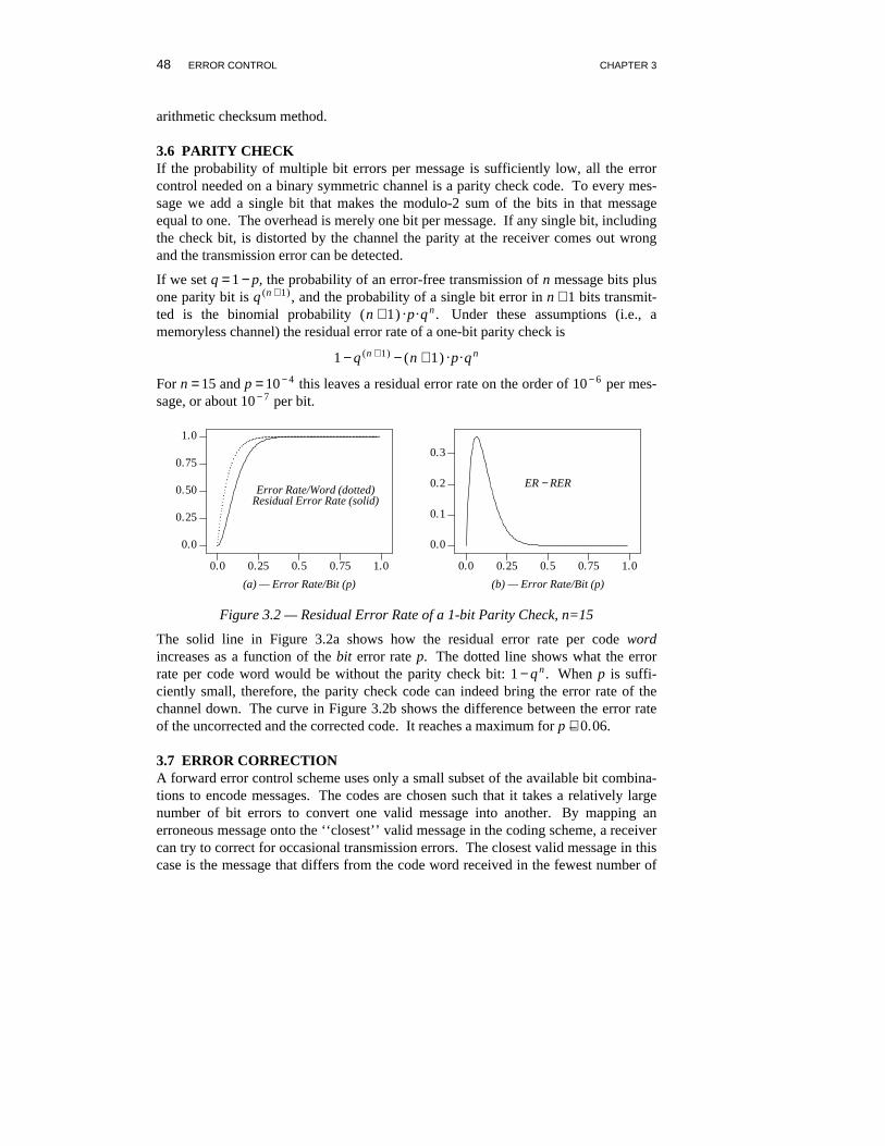
For n = 15 and p = 10 − 4 this leaves a residual error rate on the order of 10 − 6 per mes-sage, or about 10 − 7 per bit.

0. 0

0. 25

0. 50

0. 75

1. 0

0. 0 0. 25 0. 5 0. 75 1. 0

...................................................

........................................................ ...... .................... ............................................................................ ...... .

Error Rate/Word (dotted)Residual Error Rate (solid)

(a) — Error Rate/Bit (p)

0. 0

0. 1

0. 2

0. 3

0. 0 0. 25 0. 5 0. 75 1. 0

ER − RER

(b) — Error Rate/Bit (p)

Figure 3.2 — Residual Error Rate of a 1-bit Parity Check, n=15

The solid line in Figure 3.2a shows how the residual error rate per code wordincreases as a function of the bit error rate p. The dotted line shows what the errorrate per code word would be without the parity check bit: 1 − q n . When p is suffi-ciently small, therefore, the parity check code can indeed bring the error rate of thechannel down. The curve in Figure 3.2b shows the difference between the error rateof the uncorrected and the corrected code. It reaches a maximum for p ∼− 0. 06.

3.7 ERROR CORRECTIONA forward error control scheme uses only a small subset of the available bit combina-tions to encode messages. The codes are chosen such that it takes a relatively largenumber of bit errors to convert one valid message into another. By mapping anerroneous message onto the ‘‘closest’’ valid message in the coding scheme, a receivercan try to correct for occasional transmission errors. The closest valid message in thiscase is the message that differs from the code word received in the fewest number of

SECTION 3.7 ERROR CORRECTION 49

bits.

The code rate of an error-correcting code is in general lower than that of a mereerror-detecting code. In principle, therefore, forward error correction is only con-sidered to be useful when the communication of control messages from a receiverback to a sender is difficult. The difficulty may be

A very long transmission delayThe absence of a return channelA high bit-error rate

A good example of the first problem is the communication between a space probe andits remote control center on earth. A control signal, for instance to release a camerashutter or to make a course adjustment, may take several minutes to reach the distantprobe. There may not be enough time to repeat a signal in case of a transmissionerror. The signal either gets through or is lost forever.

The second problem can exist in radio broadcast transmission systems with onesender and multiple receivers. A more perverse, but very real, example is whentransmission sequences are stored on a backup-device and played back later. At thetime of transmission the original data may no longer be available for retransmission.

The third problem, a high bit error rate, may mean that even the probability that arequest for retransmission can be received correctly is unacceptably low. In all threecases, adding redundancy to a message may be the only way to avoid the irrevocableloss of some of the messages transmitted.

Even a single parity check per code word can be extended easily from a single-errordetecting code into a single-error correcting code. Every sequence of seven bits isfirst extended with a single parity bit that makes the number of one bits in eachsequence even. The parity bit is called a longitudinal redundancy check, or LRC bit.By adding an extra sequence of eight bits to every series of n codes, we can include avertical redundancy check, or VRC bit, for the set of bits that occupy the same bitposition in each sequence. For instance, with ASCII coding, for n = 4:

LRCD = 1000100 0A = 1000001 0T = 1010100 1A = 1000001 0

-------0010000 1 VRC

A faulty VRC bit encodes the column number and a faulty LRC bit the correspondingrow number for an error bit so that any single bit error per series of 40 transmitted bitscan indeed be corrected. We have used 12 check bits to protect a sequence of 28 databits, which corresponds to a code rate of 28/( 12 + 28 ) = 0. 7.

Now, let us forget about parity checks and develop an error-correcting code fromscratch. The following example is based on J.H. van Lint [1971].

50 ERROR CONTROL CHAPTER 3

EXAMPLESuppose we would like to standardize the generation of random numbers. Themethod we choose is to appoint an impartial person to be our standard randomnumber generator. He performs this task by flipping a standard coin A times persecond. The results are transmitted to all four corners of the earth via a standardbinary symmetric channel that operates at a maximum speed of 2A bps (bits persecond), with a bit error rate of 2.10 − 2.

Clearly, the result of each flip of the standard coin can be encoded in one bit of infor-mation. Transmitting the raw bits can be done at a rate of A bps, but causes thereceivers to get an average 2% of the numbers deviating from the ‘‘random stan-dard.’’

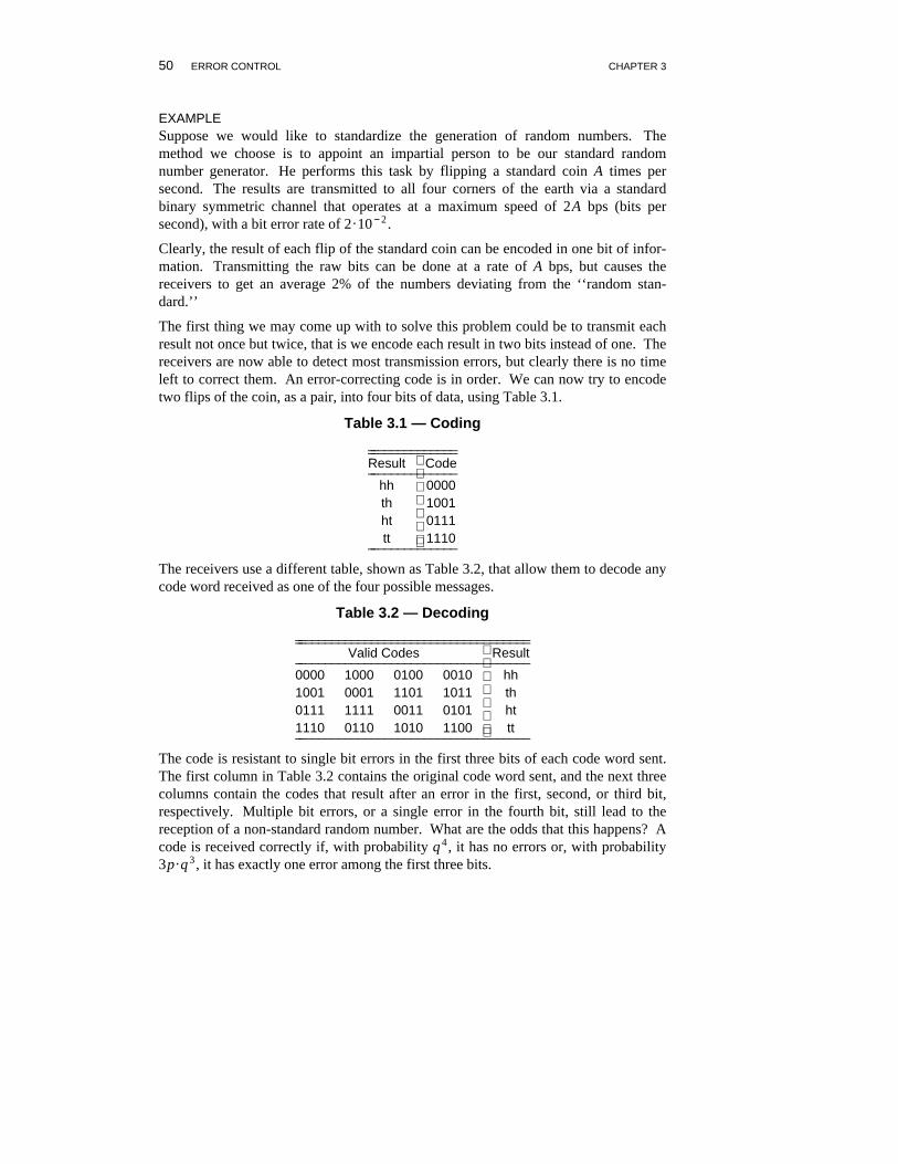
The first thing we may come up with to solve this problem could be to transmit eachresult not once but twice, that is we encode each result in two bits instead of one. Thereceivers are now able to detect most transmission errors, but clearly there is no timeleft to correct them. An error-correcting code is in order. We can now try to encodetwo flips of the coin, as a pair, into four bits of data, using Table 3.1.

Table 3.1 — Coding_ ______________ _____________Result Code_ _____________

hh 0000th 1001ht 0111tt 1110_ _____________

The receivers use a different table, shown as Table 3.2, that allow them to decode anycode word received as one of the four possible messages.

Table 3.2 — Decoding_ ____________________________________ ___________________________________

Valid Codes Result_ ___________________________________0000 1000 0100 0010 hh1001 0001 1101 1011 th0111 1111 0011 0101 ht1110 0110 1010 1100 tt_ ___________________________________

The code is resistant to single bit errors in the first three bits of each code word sent.The first column in Table 3.2 contains the original code word sent, and the next threecolumns contain the codes that result after an error in the first, second, or third bit,respectively. Multiple bit errors, or a single error in the fourth bit, still lead to thereception of a non-standard random number. What are the odds that this happens? Acode is received correctly if, with probability q 4, it has no errors or, with probability3p .q 3, it has exactly one error among the first three bits.

SECTION 3.7 ERROR CORRECTION 51

q 4 + 3p .q 3 = 0. 9788

We started out with an error rate of 2% per single bit, that is a 4% chance of at leastone error in a series of two bits. The error rate is reduced to 1 − 0. 9788 = 0. 0212 or2.12% for two subsequent bits. We used four bits to encode two flips, giving a coderate of 0. 5. We wasted twelve out of sixteen possible code words to accomplish thisreduction in the error rate, but we are still transmitting the codes as fast as the resultsare produced by our standard random number generator.

Without changing the effective signaling speed, or the code rate, we could boost theamount of waste still further by using eight bits to encode series of four data bits. Toselect the 24 valid code words needed from the range of 28 available we can againattempt to reduce the possibility that one valid word is transformed into another bytransmission errors.

HAMMING DISTANCEThe difference between two code words can be defined as the number of bits in whichthey differ. The minimum difference between two words in a code is called itsHamming distance. If we succeed in finding a code with a Hamming distance of n,any combination of up to n − 1 bit errors can be detected. Better still, any combina-tion of up to (n − 1 )/2 errors per code word can be corrected if we tell the receiver tointerpret every nonvalid code word as the closest valid code word. The receiver willguess wrong for higher numbers of bit errors, but if the probability of these is suffi-ciently low the overall error rate of the channel may still be reduced.

Formally, this method is called maximum likelihood decoding, or also nearestneighbor decoding. By increasing the Hamming distance, choosing longer and longercode words, we should then be able to increase the reliability of a code as much as wewant.

The following question now comes up: is this true for any transmission rate and forany channel? The answer can be found in a paper published by Claude Shannon in1948, A Mathematical Theory of Communication. Assuming a bandwidth limitedchannel with white noise, Shannon proved that only for transmission rates up to a cer-tain limit can the error rate of the channel be made arbitrarily small (Appendix A).The limit is called the channel capacity.

Shannon’s argument is based on the observation that the amount of informationtransferred by a channel can never exceed the entropy of the information source northe entropy of the channel itself caused by noise. Below that limit it is theoreticallyalways possible to derive reliable information from the channel. Informally, Shannonfound that when the signal-to-noise ratio gets smaller, each signal must last longer tomake it stand out from the noise, which in turn reduces the maximum signaling speedthat can be obtained.

The effort required in coding the data, however, normally prohibits the operation of achannel near the theoretical limit. For a telephone line, for instance, with a bandwidth

52 ERROR CONTROL CHAPTER 3

of 3.1 kHz and a signal-to-noise ratio of 30 dB (that is, 8:1), the Shannon limit isroughly 30 Kbit/sec, which is much more than the maximum rate used in practice.

3.8 A LINEAR BLOCK CODEWe saw in the last section that the redundancy of a code determines its power todetect and correct transmission errors. The redundancy can be defined as the numberof bits used over the minimum required to encode a message unambiguously. Toencode one of n equally likely messages, for instance, requires log 2 n bits, rounded upto the nearest integer value. We call this quantity m.

m = log 2 n

We can protect these m bits by adding c check bits and choosing the n codes usedfrom the 2(m + c) codes now available in such a way that each combination of two validcodes differs in as many bits as possible.

Table 3.3 — Parity Protection_ __________________ _________________c m m/(m+c)_ _________________1 0 0.002 1 0.503 4 0.574 11 0.735 26 0.846 57 0.907 120 0.948 247 0.97_ _________________

To be able to correct all single bit errors, we know that we need a Hamming distanceof at least three between code words, but how many check bits will this minimallycost? For every code word of m + c bits, there are precisely m + c codes that can resultfrom single bit errors. For every word from the range of 2m possible data codes,therefore, we need m + c + 1 words to protect it against single bit errors. The totalnumber of words in the code then is (m + c + 1 ) .2m, which should be equal to the2(m + c) words with which we started.Setting

(m + c + 1 ) .2m = 2(m + c)

gives

m + c + 1 = 2c

allowing us to calculate the minimal number of check bits c for any given number ofdata bits m. For m = 8, we find a minimum of c = 3. 66 or 4 check bits per message,giving a code rate of 8/( 8 + 4 ) = 0. 66.

SECTION 3.8 A LINEAR BLOCK CODE 53

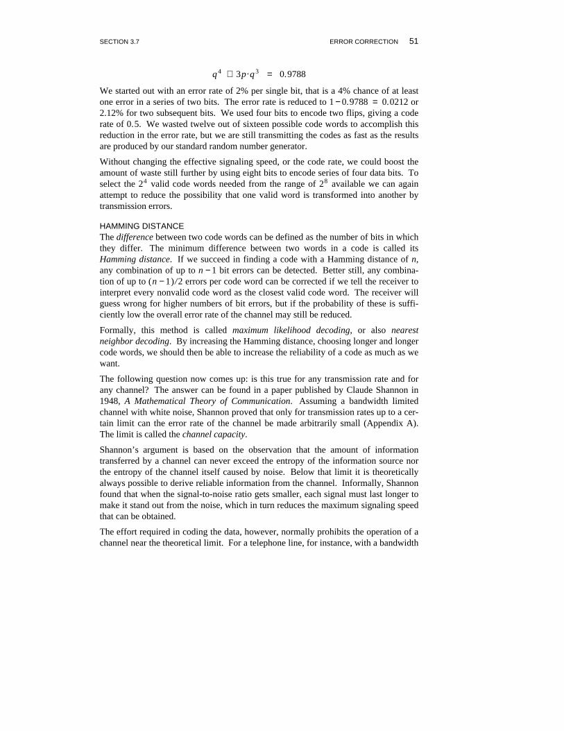
Alternatively, we can find the maximum number of data bits m for a given number ofcheck bits c. The first eight numbers are listed in Table 3.3, with the correspondingmaximum code rates. The same effect is illustrated for up to 16 checkbits in Figure3.3.

With good approximation, the number of data bits that can be protected goes upexponentially with the number of check bits that are available.

1

10

102

103

104

105

5 10 15

Maximum Number of Data Bits

(a) — Number of Check Bits

0. 0

0. 5

1. 0

5 10 15

Resulting Code Rate

(b) — Number of Check Bits

Figure 3.3 — Parity Protection

HAMMING CODEAn example of a code that realizes this protection is a code developed by R. Ham-ming. In Hamming’s code, included as an example of a perfect single-error correctingcode in Shannon’s 1948 paper, the bits in a code word are numbered from 1 to m + c.The i-th check bit is placed at the bit position 2i for 1 ≤ i ≤ log 2 (m + c).

The check bits have been placed in the code word in such a way that the sum of thebit positions they occupy points at the erroneous bit for any single bit error. To catcha single bit error the check bits are used as parity bits.

When a bit position is written as a sum of powers of two, for example, (1 + 2 + 4), italso points at the check bits that cover it. Data bit 7 = ( 1 + 2 + 4 ), for instance, iscounted in the three check bits at positions 1, 2, and 4. A single bit error that changesthe seventh data bit changes the parity of precisely these three checks. The receivercan therefore indeed determine which bit is in error by summing the bit positions ofall check bits that flagged a parity error. An error that changes, for instance, thesecond bit only affects that single bit and can also be corrected.

54 ERROR CONTROL CHAPTER 3

D: 1 0 0 0 1 0 0

D:. . . . . .

.

.

.

. . . . . . .....

0. . . . . .

.

.

.

. . . . . . .....

1 1. . . . . .

.

.

.

. . . . . . .....

0 0 0 0. . . . . .

.

.

.

. . . . . . .....

1 1 0 0

p1 p2 p4 p8

..........

...........

...........

...........

. . . . . . . . . . . . .

. . . . . . . . . . . . .

. . . . . . . . . . . . .

L:. . . . . .

.

.

.

. . . . . . .....

0. . . . . .

.

.

.

. . . . . . .....

1 1. . . . . .

.

.

.

. . . . . . .....

0 0 0 1. . . . . .

.

.

.

. . . . . . .....

1 1 0 0

..........

..........

..........

..........

..........

..........

..........

..........

..........

..........

. . . . . ..... . . . . . .

.

.

.

.1

. . . . . ..... . . . . . .

.

.

.

.0

. . . . . ..... . . . . . .

.

.

.

.1

. . . . . ..... . . . . . .

.

.

.

.1

..........

1 + 2 + 4 = 7

data

sent

received

check

error bit

Figure 3.4 — Correction of a Transmission Error

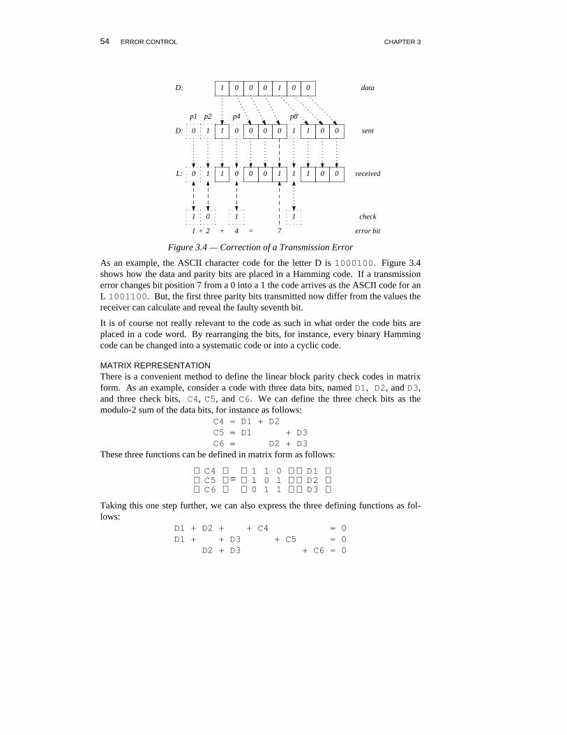
As an example, the ASCII character code for the letter D is 1000100. Figure 3.4shows how the data and parity bits are placed in a Hamming code. If a transmissionerror changes bit position 7 from a 0 into a 1 the code arrives as the ASCII code for anL 1001100. But, the first three parity bits transmitted now differ from the values thereceiver can calculate and reveal the faulty seventh bit.

It is of course not really relevant to the code as such in what order the code bits areplaced in a code word. By rearranging the bits, for instance, every binary Hammingcode can be changed into a systematic code or into a cyclic code.

MATRIX REPRESENTATIONThere is a convenient method to define the linear block parity check codes in matrixform. As an example, consider a code with three data bits, named D1, D2, and D3,and three check bits, C4, C5, and C6. We can define the three check bits as themodulo-2 sum of the data bits, for instance as follows:

C4 = D1 + D2C5 = D1 + D3C6 = D2 + D3

These three functions can be defined in matrix form as follows:

C 6C 5C 4

= 011

101

110

D 3D 2D 1

Taking this one step further, we can also express the three defining functions as fol-lows:

D1 + D2 + + C4 = 0D1 + + D3 + C5 = 0

D2 + D3 + C6 = 0

SECTION 3.8 A LINEAR BLOCK CODE 55

which leads to the following matrix representation.

011

101

110

001

010

100

. Ct = 000

In this formula, Ct is the transpose of the data word, written as a vector of bits.According to the definition, the matrix multiplication must produce a zero vector.Note that the right side of the matrix is a unit submatrix, with ones only on the diago-nal. The matrix can always be written in this form by grouping all the check bits onthe right side of the defining formulas.

H .Ct = 0

H is called a parity check matrix. Transmission errors can be formalized as an errorvector E that is added to the code word. When the receiver performs the check now,it may find a non-zero result s.

H .( Ct + E) = s

The vector s is called a syndrome. In this code every modulo-2 sum of valid codewords produces another valid code word. Therefore, if the error vector E happens tomatch any valid code word, the syndrome is zero and the error goes undetected.

BURSTSUntil now we have focused mainly on the detection and correction of single bittransmission errors, assuming that errors would be mutually independent. In practice,we know that transmission errors are not mutually independent: they tend to come inbursts.

Noise spikes, echoes, and cross-talk all affect series of subsequent bits whenever theyoccur. For a switched telephone line the average probability of a bit error may be10 − 5. But, if one bit in an arbitrary message has been distorted the probability thatthe next bit is also wrong can be as high as 0. 5. The result is that relatively few mes-sages are distorted overall, but the ones that are distorted are more seriously hurt.Clearly, it is rather pointless to develop an error control scheme that can flawlesslydetect and correct a rare single bit error if the burst errors are more common.

Though the definition of the Hamming code is relatively simple, it is surprisingly hardto extend it into a code that can correct multiple bit errors per word. To guarantee thedetection of even numbers of bit errors per code word the Hamming code can beextended with a single longitudinal parity check. A more general solution, however,is more difficult.

CODE INTERLEAVINGA general method to counter burst errors is code interleaving, One interleavingmethod is to change the order in which bits are transmitted across the channel.

Assume we have messages of n bits each, protected against single bit errors.

56 ERROR CONTROL CHAPTER 3

Assuming further that traffic is non-interactive, we can intercept burst errors up to alength of k bits by buffering each block of k subsequent messages, placing them in amatrix of k×n bits and transmitting the bits in this matrix column by column insteadof row by row. At the receiver end the original matrix is restored column by columnand read row by row. A burst error of length k or less then only causes a single biterror per row and can be corrected properly.

True double-error correcting codes, not based on interleaving schemes, were first pub-lished by Hocquenghem [1959], and Bose and Ray-Chaudhuri [1960]. These codes,collectively known as BCH codes, require substantially more theoretical justificationthan can be given here. A further generalization of the BCH codes is known as theReed-Solomon code. It has found application, for instance, in the digital encoding ofsound on compact disks.

In a study performed at IBM in 1964, it was found that in almost all cases feedbackerror control can be superior to forward error control in both throughput and in resi-dual error rates. We therefore continue with a discussion of a cyclic block code that isused for feedback error control.

3.9 CYCLIC REDUNDANCY CHECKSThe cyclic redundancy check, or CRC, method is also based on the addition of seriesof check bits to code words. In this case the added bits guarantee that, in the absenceof transmission errors, the code word plus check bits is divisible by a given factor.The specific division method and the factor used determine the range of transmissionerrors that can be detected. To simplify the algebraic manipulation of code words wecan define a mapping of codes onto polynomials. A sequence of N bits can then beinterpreted as a polynomial of maximum degree N − 1:

i = 0Σ

N − 1

b i.x i

where each b i takes the value of the bit in position i in the sequence, with bits num-bered right to left. The code word 10011, for instance, defines polynomial

x 4 + x + 1

We are working in a binary system so all operations, including division and multipli-cation, are defined modulo-2. Modulo-2 addition is defined as follows:

0 + 0 = 0 - 0 = 0

0 + 1 = 0 - 1 = 1

1 + 0 = 1 - 0 = 1

1 + 1 = 1 - 1 = 0

In longer additions there is no carry, and in subtractions there is no borrow. In poly-nomial form, therefore, for any i we have x i + x i = 0, since both 1 + 1 = 0 and0 + 0 = 0. To multiply two code words, we can multiply the corresponding polynomi-als.

SECTION 3.9 CYCLIC REDUNDANCY CHECKS 57

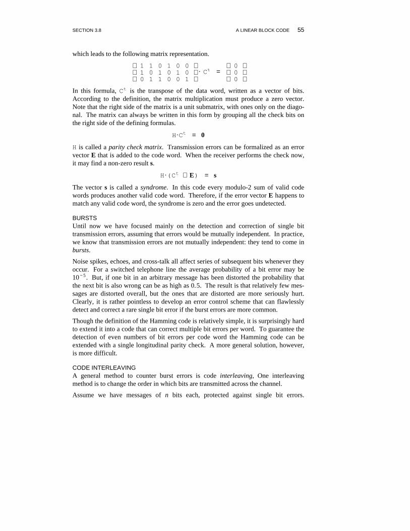
Table 3.4 — A Cyclic Code_ _________________________________________________________________ ________________________________________________________________Data Word Polynomial Multiplied By Produces Code Word_ ________________________________________________________________0 0 0 0 x + 1 0 0 0 0 0

0 0 1 1 x + 1 x + 1 0 0 1 1

0 1 0 x x + 1 x 2 + x 0 1 1 0

0 1 1 x + 1 x + 1 x 2 + 1 0 1 0 1

1 0 0 x 2 x + 1 x 3 + x 2 1 1 0 0

1 0 1 x 2 + 1 x + 1 x 3 + x 2 + x + 1 1 1 1 1

1 1 0 x 2 + x x + 1 x 3 + x 1 0 1 0

1 1 1 x 2 + x + 1 x + 1 x 3 + 1 1 0 0 1_ ________________________________________________________________

For example,

(x 4 + x + 1 ) × (x 3 + x 2 ) = x 7 + x 6 + x 4 + x 2

We can use this mechanism easily to define a code. Consider, for instance, a codewith three data bits. We encode the data in four bits by multiplying every data wordwith the polynomial x + 1, as shown in Table 3.4. The resulting code is a parity checkcode with a code rate of 3/4. It is also a cyclic code, but not a systematic one.

If we can add, subtract and multiply polynomials, we can of course also divide them.Let us try dividing the polynomial x 7 + x 6 + x 3 + x 4 + x 2 by a factor x 5 + x 2 + 1.

x 5 + x 2 + 1 / x 7 + x 6 + x 4 + x 3 + x 2 \ x 2 + x

x 6 + 0 + x 3x 7 + 0 + x 4 + 0 + x 2_ ________________

xx 6 + 0 + x 3 + x_ ____________

To make the original polynomial divisible by factor x 5 + x 2 + 1, we could simply sub-tract the residual x from it. But, although the receiver would then be able to detecttransmission errors, it would not be able to recover the original message from thecode word. Better is to append the residual as a checksum. The factor used to gen-erate a checksum is called the generator polynomial of the code.

We now first multiply the message polynomial by a factor equal to the highest degreeof the generator polynomial, in this case x 5, to make room for the checksum. It sim-ply means shifting the bits in the code word five places to the left. Then we divide themessage polynomial by the generator polynomial and subtract the residual.

Since the CRC is a linear code, every error pattern E must be equal to some valid codeword T. For a known code this property can be used to calculate the residual errorrate. If P is the message polynomial and G a generator polynomial of degree r, theresidual R has degree r − 1 and is defined to be the remainder of

GP .xr_ ____

% ERROR CONTROL CHAPTER 3

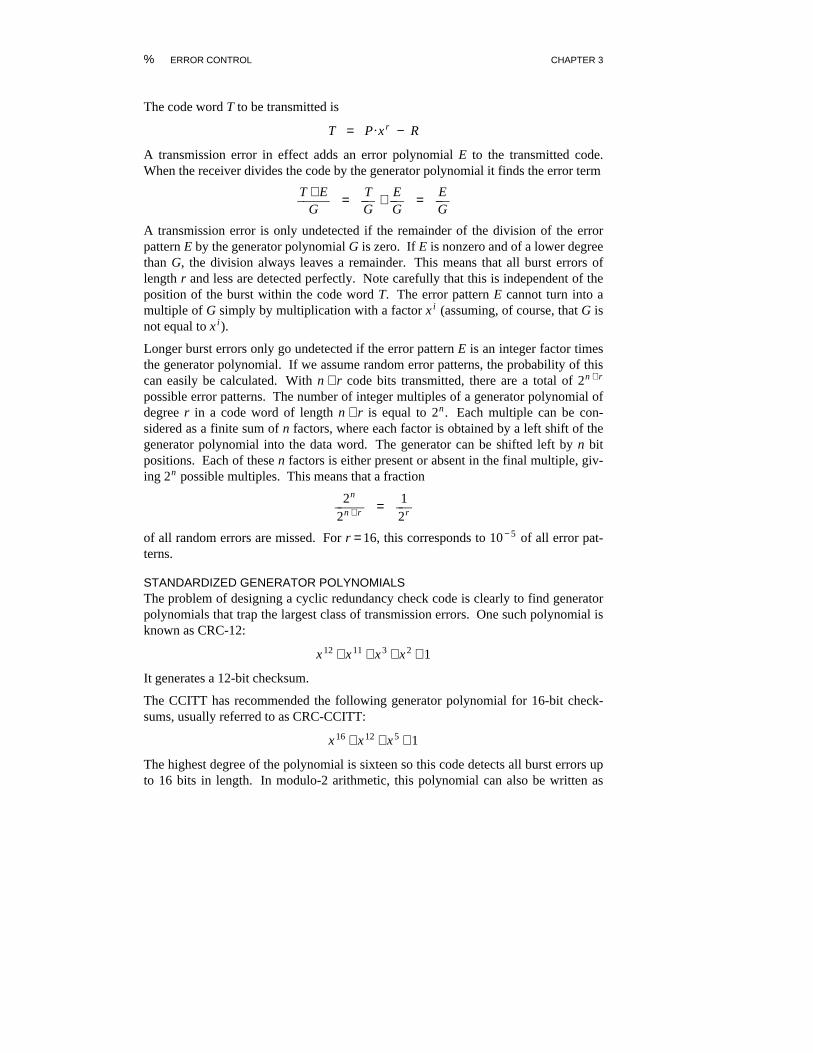
The code word T to be transmitted is

T = P .xr − R

A transmission error in effect adds an error polynomial E to the transmitted code.When the receiver divides the code by the generator polynomial it finds the error term

GT + E_ ____ =

GT_ __ +

GE_ __ =

GE_ __

A transmission error is only undetected if the remainder of the division of the errorpattern E by the generator polynomial G is zero. If E is nonzero and of a lower degreethan G, the division always leaves a remainder. This means that all burst errors oflength r and less are detected perfectly. Note carefully that this is independent of theposition of the burst within the code word T. The error pattern E cannot turn into amultiple of G simply by multiplication with a factor x i (assuming, of course, that G isnot equal to x i).

Longer burst errors only go undetected if the error pattern E is an integer factor timesthe generator polynomial. If we assume random error patterns, the probability of thiscan easily be calculated. With n + r code bits transmitted, there are a total of 2n + r

possible error patterns. The number of integer multiples of a generator polynomial ofdegree r in a code word of length n + r is equal to 2n . Each multiple can be con-sidered as a finite sum of n factors, where each factor is obtained by a left shift of thegenerator polynomial into the data word. The generator can be shifted left by n bitpositions. Each of these n factors is either present or absent in the final multiple, giv-ing 2n possible multiples. This means that a fraction

2n + r2n

_ ____ =2r1_ __

of all random errors are missed. For r = 16, this corresponds to 10 − 5 of all error pat-terns.

STANDARDIZED GENERATOR POLYNOMIALSThe problem of designing a cyclic redundancy check code is clearly to find generatorpolynomials that trap the largest class of transmission errors. One such polynomial isknown as CRC-12:

x 12 + x 11 + x 3 + x 2 + 1

It generates a 12-bit checksum.

The CCITT has recommended the following generator polynomial for 16-bit check-sums, usually referred to as CRC-CCITT:

x 16 + x 12 + x 5 + 1

The highest degree of the polynomial is sixteen so this code detects all burst errors upto 16 bits in length. In modulo-2 arithmetic, this polynomial can also be written as

SECTION 3.9 CYCLIC REDUNDANCY CHECKS 59

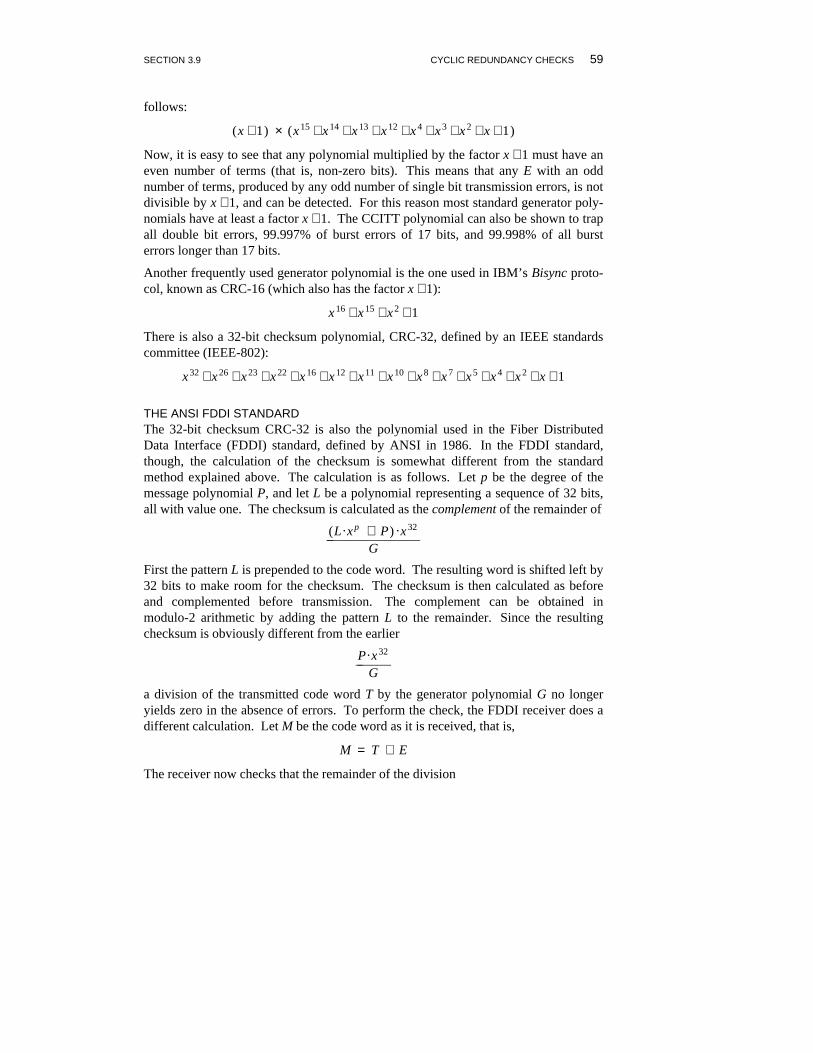
follows:

(x + 1 ) × (x 15 + x 14 + x 13 + x 12 + x 4 + x 3 + x 2 + x + 1 )

Now, it is easy to see that any polynomial multiplied by the factor x + 1 must have aneven number of terms (that is, non-zero bits). This means that any E with an oddnumber of terms, produced by any odd number of single bit transmission errors, is notdivisible by x + 1, and can be detected. For this reason most standard generator poly-nomials have at least a factor x + 1. The CCITT polynomial can also be shown to trapall double bit errors, 99.997% of burst errors of 17 bits, and 99.998% of all bursterrors longer than 17 bits.

Another frequently used generator polynomial is the one used in IBM’s Bisync proto-col, known as CRC-16 (which also has the factor x + 1):

x 16 + x 15 + x 2 + 1

There is also a 32-bit checksum polynomial, CRC-32, defined by an IEEE standardscommittee (IEEE-802):

x 32 + x 26 + x 23 + x 22 + x 16 + x 12 + x 11 + x 10 + x 8 + x 7 + x 5 + x 4 + x 2 + x + 1

THE ANSI FDDI STANDARDThe 32-bit checksum CRC-32 is also the polynomial used in the Fiber DistributedData Interface (FDDI) standard, defined by ANSI in 1986. In the FDDI standard,though, the calculation of the checksum is somewhat different from the standardmethod explained above. The calculation is as follows. Let p be the degree of themessage polynomial P, and let L be a polynomial representing a sequence of 32 bits,all with value one. The checksum is calculated as the complement of the remainder of

G(L .xp + P) .x 32_ ______________

First the pattern L is prepended to the code word. The resulting word is shifted left by32 bits to make room for the checksum. The checksum is then calculated as beforeand complemented before transmission. The complement can be obtained inmodulo-2 arithmetic by adding the pattern L to the remainder. Since the resultingchecksum is obviously different from the earlier

GP .x 32_ _____

a division of the transmitted code word T by the generator polynomial G no longeryields zero in the absence of errors. To perform the check, the FDDI receiver does adifferent calculation. Let M be the code word as it is received, that is,

M = T + E

The receiver now checks that the remainder of the division

60 ERROR CONTROL CHAPTER 3

G(L .xp + M) .x 32_ ______________

equals

GL .x 32_ _____

that is, it must equal the pattern L that was added to the checksum at the FDDI senderto invert it before the transmission. The addition of the pattern L and the inversion ofthe checksum guarantee, among other things, that a transmitted code word never con-sists of only zero bits.

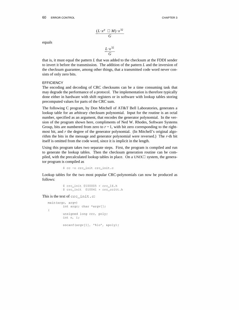
EFFICIENCYThe encoding and decoding of CRC checksums can be a time consuming task thatmay degrade the performance of a protocol. The implementation is therefore typicallydone either in hardware with shift registers or in software with lookup tables storingprecomputed values for parts of the CRC sum.

The following C program, by Don Mitchell of AT&T Bell Laboratories, generates alookup table for an arbitrary checksum polynomial. Input for the routine is an octalnumber, specified as an argument, that encodes the generator polynomial. In the ver-sion of the program shown here, compliments of Ned W. Rhodes, Software SystemsGroup, bits are numbered from zero to r − 1, with bit zero corresponding to the right-most bit, and r the degree of the generator polynomial. (In Mitchell’s original algo-rithm the bits in the message and generator polynomial were reversed.) The r-th bititself is omitted from the code word, since it is implicit in the length.

Using this program takes two separate steps. First, the program is compiled and runto generate the lookup tables. Then the checksum generation routine can be com-piled, with the precalculated lookup tables in place. On a UNIX system, the genera-tor program is compiled as

$ cc -o crc_init crc_init.c

Lookup tables for the two most popular CRC-polynomials can now be produced asfollows:

$ crc_init 0100005 > crc_16.h$ crc_init 010041 > crc_ccitt.h

This is the text of crc_init.c:

main(argc, argv)int argc; char *argv[];

{unsigned long crc, poly;int n, i;

sscanf(argv[1], "%lo", &poly);

SECTION 3.9 CYCLIC REDUNDANCY CHECKS 61

if (poly & 0xffff0000){ fprintf(stderr, "polynomial is too large\n");

exit(1);}

printf("/*\n * CRC 0%o\n */\n", poly);printf("static unsigned short crc_table[256] = {\n");for (n = 0; n < 256; n++){ if (n % 8 == 0) printf(" ");

crc = n << 8;for (i = 0; i < 8; i++){ if (crc & 0x8000)

crc = (crc << 1) ˆ poly;else

crc <<= 1;crc &= 0xFFFF;

}if (n == 255) printf("0x%04X ", crc);else printf("0x%04X, ", crc);if (n % 8 == 7) printf("\n");

}exit(0);

}

The table can now be used to generate checksums:

unsigned shortcksum(s, n)

register unsigned char *s;register int n;

{register unsigned short crc=0;

while (n-- > 0)crc = crc_table[(crc>>8 ˆ *s++) & 0xff] ˆ (crc<<8);

return crc;}

The CRC checksum, using a lookup table with the algorithm shown above, is com-puted in approximately 1.1 msec of CPU time (for a 512-bit message, when runningon a DEC/VAX-750). For comparison, the following is the checksum routine fromthe UNIX system uucp code.

cksum(s,n)register char *s;register n;

{register short sum;register unsigned short t;register short x;

62 ERROR CONTROL CHAPTER 3

sum = -1;x = 0;

do {if (sum<0) {

sum <<= 1;sum++;

} elsesum <<= 1;

t = sum;sum += (unsigned)*s++ & 0377;x += sumˆn;if ((unsigned short)sum <= t) {

sum ˆ= x;}

} while (--n > 0);

return(sum);}

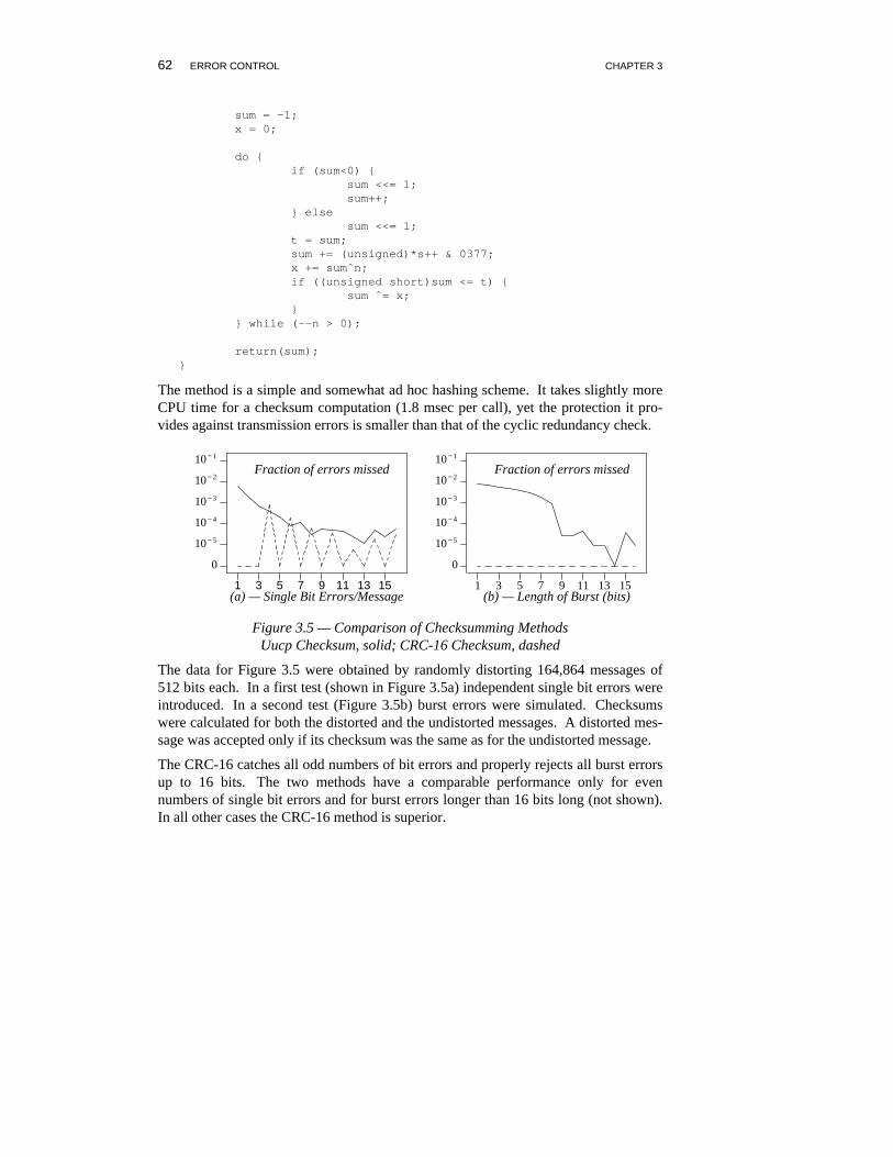
The method is a simple and somewhat ad hoc hashing scheme. It takes slightly moreCPU time for a checksum computation (1.8 msec per call), yet the protection it pro-vides against transmission errors is smaller than that of the cyclic redundancy check.

10− 1

10− 2

10− 3

10− 4

10− 5

0

1 3 5 7 9 11 13 15(a) — Single Bit Errors/Message

Fraction of errors missed10− 1

10− 2

10− 3

10− 4

10− 5

0

1 3 5 7 9 11 13 15(b) — Length of Burst (bits)

Fraction of errors missed

Figure 3.5 — Comparison of Checksumming MethodsUucp Checksum, solid; CRC-16 Checksum, dashed

The data for Figure 3.5 were obtained by randomly distorting 164,864 messages of512 bits each. In a first test (shown in Figure 3.5a) independent single bit errors wereintroduced. In a second test (Figure 3.5b) burst errors were simulated. Checksumswere calculated for both the distorted and the undistorted messages. A distorted mes-sage was accepted only if its checksum was the same as for the undistorted message.

The CRC-16 catches all odd numbers of bit errors and properly rejects all burst errorsup to 16 bits. The two methods have a comparable performance only for evennumbers of single bit errors and for burst errors longer than 16 bits long (not shown).In all other cases the CRC-16 method is superior.

SECTION 3.10 ARITHMETIC CHECKSUM 63

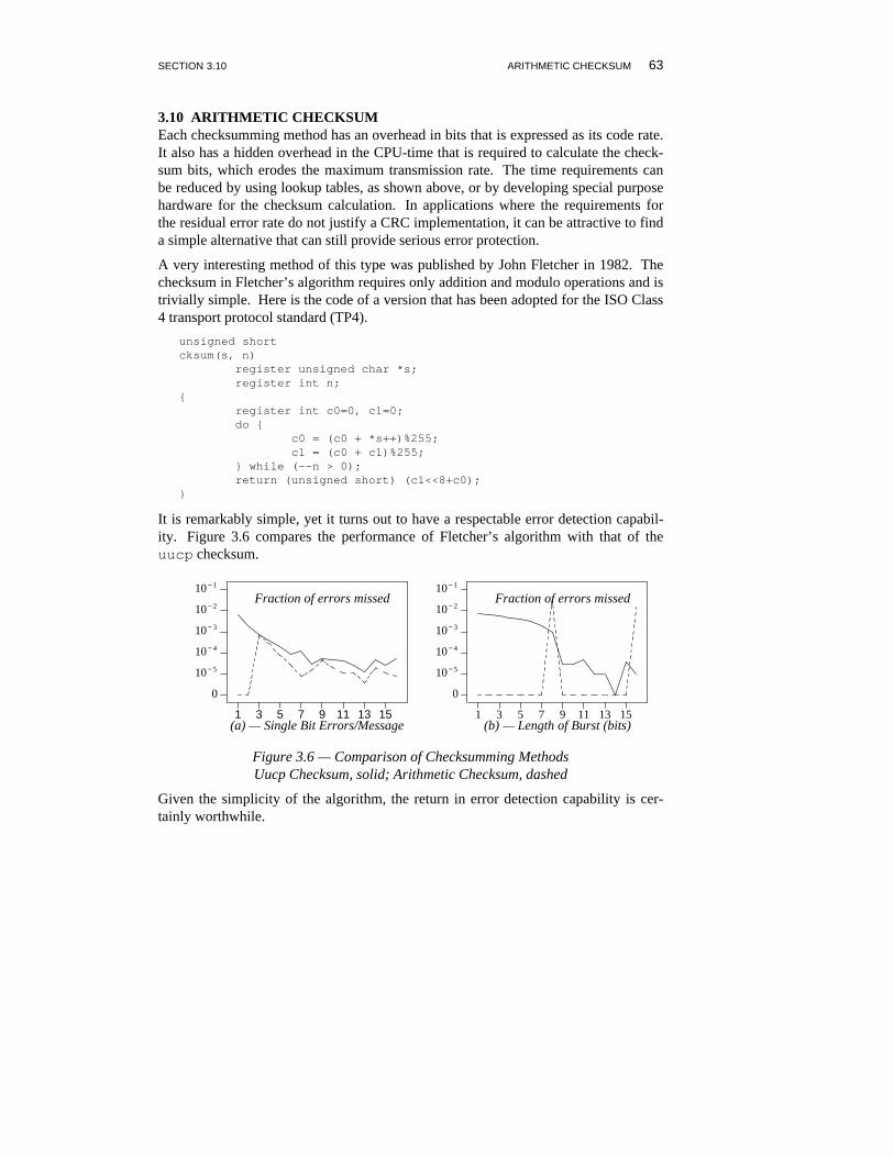
3.10 ARITHMETIC CHECKSUMEach checksumming method has an overhead in bits that is expressed as its code rate.It also has a hidden overhead in the CPU-time that is required to calculate the check-sum bits, which erodes the maximum transmission rate. The time requirements canbe reduced by using lookup tables, as shown above, or by developing special purposehardware for the checksum calculation. In applications where the requirements forthe residual error rate do not justify a CRC implementation, it can be attractive to finda simple alternative that can still provide serious error protection.

A very interesting method of this type was published by John Fletcher in 1982. Thechecksum in Fletcher’s algorithm requires only addition and modulo operations and istrivially simple. Here is the code of a version that has been adopted for the ISO Class4 transport protocol standard (TP4).

unsigned shortcksum(s, n)

register unsigned char *s;register int n;

{register int c0=0, c1=0;do {

c0 = (c0 + *s++)%255;c1 = (c0 + c1)%255;

} while (--n > 0);return (unsigned short) (c1<<8+c0);

}

It is remarkably simple, yet it turns out to have a respectable error detection capabil-ity. Figure 3.6 compares the performance of Fletcher’s algorithm with that of theuucp checksum.

10− 1

10− 2

10− 3

10− 4

10− 5

0

1 3 5 7 9 11 13 15(a) — Single Bit Errors/Message

Fraction of errors missed10− 1

10− 2

10− 3

10− 4

10− 5

0

1 3 5 7 9 11 13 15(b) — Length of Burst (bits)

Fraction of errors missed

Figure 3.6 — Comparison of Checksumming MethodsUucp Checksum, solid; Arithmetic Checksum, dashed

Given the simplicity of the algorithm, the return in error detection capability is cer-tainly worthwhile.

64 ERROR CONTROL CHAPTER 3

3.11 SUMMARYOne functional module in the protocol hierarchy is error control. The inclusion of anerror control scheme can and should be transparent to the rest of the protocol. Itsfunction is to transform a channel with error rate p into one with a lower (residual)error rate p .( 1 − f ), where f is the fraction of the errors that is intercepted by the errorcode.

An error control scheme requires overhead that is measured by the number of redun-dant bits that are added to each code word. Redundancy is rarely equal to protection(see Exercise 3-1), but a small amount of redundancy is a prerequisite to any errorcontrol scheme.

With proper encoding and at the price of lower transfer rates, the receiver can use anerror-correcting code to recover from the characteristic errors introduced by the chan-nel. With lower overhead an acceptable performance can be achieved with error-detecting codes that rely on flow control schemes for the retransmission of distorteddata. Flow control schemes are studied in Chapter 4.

The adequacy of an error control scheme, however, can only be assessed properlywhen the error characteristics of the transmission channel, the required transfer rate(i.e., code rate), and the required level for the residual error rate are known.

EXERCISES

3-1. 3-1. A phone company recently considered running new 56 Kbit/sec data lines at an end-to-end data rate of 9600 bits/sec, using the extra bandwidth to enhance reliability. Themethod chosen was to transmit each single byte five times in succession. By a majorityvote, comparing the five successive bytes and choosing the most frequent one from eachset, the receiver would then decide which byte had been transmitted. Comment on thecode rate and the protection against burst errors.

3-2. 3-2. A simple error control scheme has the receiver retransmit all the messages it receivesback to the sender. Each message then has to survive two successive transmissions to beaccepted. Try to build a protocol that works this way.

3-3. 3-3. The protocol of Exercise 3-2 is modified to have the receiver merely return a CRC check-sum field to the sender by way of acknowledgment. The checksum is returned for everymessage received, distorted or not, and is used by the sender to decide upon retransmis-sion. Comment upon this improvement.

3-4. 3-4. (Jon Bentley) The two sentences ‘‘the dog runs’’ and ‘‘the dogs run’’ are both valid inEnglish. The sentences ‘‘the dogs runs’’ and ‘‘the dog run’’ are both invalid. Would thisclassify English grammar as a feedback or as a forward error control method?

3-5. 3-5. The message 101011000110 is protected by a CRC checksum that was generated withthe polynomial x 6 + x 4 + x + 1. The checksum is in the tail (the right side) of themessage. (a) How many bits is the checksum? (b) If no transmission errors occurred,what would the original data be? (c) Were there any transmission errors?

3-6. 3-6. List the circumstances under which an error-correcting code with a code rate of 0.1 canbe more attractive than an error-detecting code with feedback error control? Considererror rates and roundtrip message propagation delays.

CHAPTER 3 BIBLIOGRAPHIC NOTES 65

3-7. 3-7. Another method to adapt a single error-correcting code for protection against burst errorsis to use n error codes for a sequence of n messages, where the i-th code word coversonly the i-th bit from each message. To protect against burst errors of up to k bits thismethod attempts to separate the bits that make up one new ‘‘code word,’’ spanning nmessages, by more than k bit positions. Work out the details of this method and apply itto a sample message.

3-8. 3-8. CRC checksum polynomials that contain the factor x + 1 catch all odd numbers of biterrors. Think of a method to catch all even numbers of bit errors as well, for instance, bydeliberately introducing a bit error in a second transmission, and comment upon thisscheme. Consider the code rate as well.

3-9. 3-9. How would you classify Fletcher’s algorithm? (See Section 3.4)

BIBLIOGRAPHIC NOTESMore information on the various types of transmission errors and their causes can befound in, for instance, Tanenbaum [1981, 1988], Fleming and Hutchinson [1971], andBennet and Davey [1965]. An application oriented treatment of data transmissiontechniques can be found in Tugal and Tugal [1982].

The Hamming code was first described by Claude Shannon [1948] as an example of aperfect code. Hamming’s paper on error-correcting codes followed a few years later,Hamming [1950]. Slepian [1973] gives an overview of the theory inspired byShannon’s work. An excellent introduction to coding theory can be found in J.H. vanLint’s lecture notes, Lint [1971].

Other good reference works on the theory of error-correcting and error-detectingcodes, including discussions of BCH and Reed-Solomon codes, are Berlekamp[1968], Kuo [1981], Peterson and Weldon [1972], and MacWilliams and Sloane[1977]. The results of the IBM study of error-correcting and error-detecting codes,mentioned at the conclusion of Section 3.7, were presented in IBM [1964]. A simplemethod to generate a CRC lookup table was described in Perez [1983]. Alternativemethods to generate CRC-16 and CRC-32 checksums using look-ahead tables can befound in Griffiths and Stones [1987]. Methods to generate CRC checksums with shiftregisters are given in e.g., MacWilliams and Sloane [1977], Adi [1984], and Stallings[1985].

The results of a survey held in 1969-1970 to measure the error characteristics ofswitched lines was reported in Fleming and Hutchinson [1971] and Balkovic et al.[1971]. An overview of the results of measurements on T1 lines, performed byAT&T in 1973 and 1974, is given in Brilliant [1978]. More general discussions orvarious ways for interpreting and analyzing the measurement data can be found in, forinstance, Decina and Julio [1982] or in Ritchie and Scheffler [1982].

Fletcher’s arithmetic checksumming method was first described in Fletcher [1982],and is discussed in Nakassis [1988]. The ISO transport protocol series was standard-ized in ISO [1983]. The predictive model for error clustering, discussed in Section3.2 is described in Bond [1987] and is due to Benoit Mandelbrot [1965] (the inventorof fractals).