Error Bounds for Linear Recurrence Relations*...1. Introduction. The application of mth order linear recurrence relations (1.1) ar0Pr + arlPr-l + ar2pr-2 -\-h OrmPr-m + dr = 0, in

$Page 1: Error Bounds for Linear Recurrence Relations*...1. Introduction. The application of mth order linear recurrence relations (1.1) ar0Pr + arlPr-l + ar2pr-2 -\-h OrmPr-m + dr = 0, in$
MATHEMATICS OF COMPUTATIONVOLUME 50, NUMBER 182APRIL 1988, PAGES 481-499

Error Bounds for Linear Recurrence Relations*

By F. W. J. Olver

Abstract. Recurrence relations of the form

O-rPr+1 = brpr + CrPr-1

are examined in two cases: (A) oscillatory systems, for which b% + 4arcr < 0; (B)

monotonie systems, for which bl¡. + 4arcr > 0. In both cases, a posteriori methods are

supplied for constructing strict and realistic error bounds in 0(r) arithmetic operations.

A priori bounds, also requiring 0(r) arithmetic operations, are supplied in Case B.

Several illustrative numerical examples are included.

1. Introduction. The application of mth order linear recurrence relations

(1.1) ar0Pr + arlPr-l + ar2pr-2 -\-h OrmPr-m + dr = 0,

in which or0 ^ 0, all r, to generate a sequence of values pm, pm+i,... from pre-

scribed values of po,pi,... ,pm-i is a well-understood procedure in numerical anal-

ysis. See, for example, [1], [2], [3], [4] and, most recently, the monograph of Wimp

[19]. If the corresponding homogeneous equation is regarded as a difference equa-

tion, then it has m linearly independent solutions—the so-called complementary

functions of (1.1). Each rounding error introduced in the recurrence process con-

taminates the wanted solution of (1.1) by small multiples of the complementary

functions. This is of no concern if the wanted solution grows in size at least as

fast as any of the complementary functions, that is, if it is a dominant solution. In

other cases the process may fail, indeed fail disastrously, and in order to achieve

stability it is necessary to apply the recurrence relation in a backward direction, or

to solve a boundary value problem.

Perhaps because stability conditions are so well understood, comparatively little

attention has been paid to the problem of constructing strict error bounds for

the computed results. These bounds are to cover the effects of rounding errors

introduced during the recurrence steps as well as inherent errors in the coefficients

arj and dr and the initial values Po,Pi, • • • ,pm-i- This is the problem treated in

the present investigation. One obvious application is to the development of robust

software for the generation of transcendental mathematical functions by recurrence.

The only relevant published work appears to be that for Miller's algorithm; see

[7], [9], [16]. In fact, some results for the present problem could be found simply

by specializing results given in these references, especially [7]. This approach leads

to unnecessary complications, however, and a more direct attack is called for.

Received October 30, 1986, revised July 6, 1987.

1980 Mathematics Subject Classification (1985 Revision). Primary 65Q05; Secondary 65G05.

"This research has been supported by the U. S. Army Research Office, Durham under Contract

DAAG-29-84-K-0022, the U. S. National Science Foundation under Grant DMS-84-19820 and theII. K. Science and Engineering Research Council.

©1988 American Mathematical Society

0025-5718/88 $1.00 + $.25 per page

481

License or copyright restrictions may apply to redistribution; see https://www.ams.org/journal-terms-of-use

482 F. W. J. OLVER

We first observe that the evaluation of pr for the range r = m, m+1,..., m+n—1,

say, is equivalent to the solution of a system of n linear algebraic equations. Hence

the required error bounds can be found by available algorithms in matrix algebra;

see, for example, [13], [14]. A drawback to this approach is that it requires the

inversion of a lower triangular band matrix. The number of arithmetic operations

needed for the inversion is 0(n2), for large n, compared with only O(n) operations

for the computation of the solution pr. It can be argued that it suffices to have the

norm of the inverse matrix. However, it is an upper bound for the norm that is

really needed, and this is tantamount to the original problem.1

Another drawback to the matrix approach is that it usually fails to provide

insight into the nature of the error bounds; in particular, it will not yield realistic

bounds of a priori type unless, of course, bounds for the elements or norm of the

inverse matrix are known.

A second general approach is to apply rounded interval arithmetic [8, Section

2.4]. Often this procedure is quite successful. In many cases, however, the computed

intervals are absurdly unrealistic. We illustrate this observation by two simple

examples.

Example 1.1.

(1.2) 12pr+1=25pr-13pr_i; po = 1, pi = 13/12.

Computed interval values of P2,P3, • • • ,Pi6 are given in Table 1.1. For example,

the entries for r = 2 mean that

1.17360 < p2 < 1.17363.

Six-figure decimal arithmetic was employed, with directed rounding2 applied im-

mediately following each arithmetic operation at each recurrence step.

Clearly the interval widths grow rapidly as r increases. After r = 12 the left

endpoint begins to decrease and actually becomes negative at r = 16, even though

the true solution pr = (13/12)r is positive, increasing and dominant.

Example 1.2.

(1.3) 3pr+i - V22pr + 2pr_i -1 = 0; po = pi = 1.

An interval solution was computed in the same manner as Example 1.1, and the

results are presented in Table 1.2. Again the interval widths grow rapidly with

r, even though the wanted solution is dominant and tends to the constant value

3.23013... as r —> oo. The actual solution is given by

pr = |(5 + >/22) - 2r/23_(r+2)/2{(2 + v/22) cosroj + (VyK - y/EÖ) sinrw},

with u = tan-1 (l/\/ïï).

'Compare [5]. Here algorithms are supplied for computing the norm of the inverse of a tridi-

agonal matrix of order n in 0(n) operations. The algorithms entail the application of three-term

homogeneous recurrence relations.

2That is, towards —oo for left endpoints and towards +00 for right endpoints.


ERROR BOUNDS FOR LINEAR RECURRENCE RELATIONS 483

r

0

1

2

3

4

56

7

8

910

11

12

13

14

15

16

TABLE 1.1

Interval solution of (1

- Pr -1

2)

1.083331.173601.27137

1.377251.49183

1.61568

1.74914

1.89194

2.04215

2.193592.32926

2.404882.307381.75065

0.01335834.72027

11.08334

1.17363

1.27147

1.377501.492481.617321.753281.902352.068342.259452.494872.82127

3.354304.38285

6.6313511.9189

IPr+l/IPr

3.0

3.333...2.52.62.523...2.524...2.514...

2.515...2.514...

2.514...2.514...

2.514...2.514...

2.514...

2.514...

r

01

2

34

5

678

910

11

12

13

1415

16

Table 1.2

Interval solution of (

I- Pr -,

1

11.23013

1.589931.99904

2.398792.75102

3.035173.244473.38203

3.457163.48206

3.469333.429803.370703.29356

3.19116

1

1

1.230141.58996

1.999112.39894

2.75134

3.035813.245763.384573.462073.491543.487503.46460

3.437303.42094

3.43477

1.3)

IPr+l/Ipr

3.02.333..2.142..

2.133..2.02.015..1.968..1.933..1.930..1.916..1.915..1.913..

1.912..1.912..

The explanation of the failure of interval arithmetic in these examples is the usual

one: the process takes no account of the interdependence of errors at successive

steps. In fact, in Example 1.1 the interval widths Ipr, say, eventually grow in

proportion to aT, where a = 2.514... is the largest zero of the polynomial 1222 —

25z — 13. This is confirmed by the numerical values of the ratio Jpr+i/Jpr given

in the final column of Table 1.1. Similarly in Example 1.2 the interval widths

eventually grow in proportion to ar, where a = 1.912... is the largest zero of

3z2 - yffiz - 2.To construct methods that entail no more than 0(r) arithmetic operations and

yield realistic error bounds, we have to impose restrictions on the nature of the

recurrence relation. Without such restrictions, we have only the general matrix

approach, with its 0(r2) operations, to fall back on for realistic bounds. The

present paper treats only real second-order relations. We also restrict ourselves

to homogeneous systems, mainly because inhomogeneous problems often require

error bounds for the associated complementary functions as a necessary preliminary

[1], [10], [19]. In some cases, however, our methods carry over straightforwardly

to inhomogeneous systems. Admittedly, the problems that fall within our scope

amount to only a small subclass of the general problem of solving linear difference

equations; nevertheless, this subclass includes many important recurrence relations

satisfied by the higher transcendental functions.

We standardize (1.1) for homogeneous second-order systems in the form

(1.4) arpr+i = brpr + crpr_i,

with po and pi prescribed and ar ^ 0, all r. We distinguish two cases: oscillatory

systems in which b2 + 4arcr is negative for all r, and monotonie systems in which

b2 + AarcT is nonnegative for all r. This classification is suggested, of course, by the

nature of the solutions when the ar, br and cr are constants. Oscillatory systems

are treated in Section 2, and monotonie systems in Sections 3, 4 and 5. In both

cases we provide methods for constructing error bounds of a posteriori type. For


484 F. W. J. OLVER

monotonie systems we also furnish a priori bounds. Some numerical examples are

supplied in Section 6, and brief conclusions are drawn in Section 7.

2. Oscillatory Systems. In (1.4) we replace cr by —cr for convenience. The

oscillatory case is then given by

(2.1) arpr+1 = brpr - Crpr-i,

with b2 < 4arcr, all r. Without loss of generality we may suppose that ar and cr

are positive.

Example 1.2 is typical for systems of this kind in that interval arithmetic will

generally yield unsatisfactory results. The error bounds, or interval widths, even-

tually grow at the same rate as the dominant solution of the equation

arpr+i = \br\pr +crpr-i.

That this solution grows faster than the solutions of (2.1) can be inferred from the

case in which the coefficients are constants.

In order to proceed, let qr be a solution of (2.1) that is independent of pr and

(like pr) is computed by forward recurrence from given values at r = 0 and 1.

Denote the stored values of pr, qr and other quantities by the addition of overbars.

Also, let 4>r and ipr be the aggregate errors introduced on the (r — l)st step in the

computation of pr and qr, as expressed by the formulae

(2.2) ar-ipr =br-ipr-i-cr-ipr-2 + (pr, ar-iqr = bT-iqr-i-cr-iqr-2+il>r-

Thus (pr includes the effects of all abbreviation errors3 introduced in the computa-

tion of pr from pr_i and pr-2 as well as the effects of inherent errors in the given

values of the coefficients ar_i, br-i and cr-i. Similarly for tpr.

Bounds for \(pr\ and |t/v| can be computed by standard methods of round-off

error analysis, see for example [12], [18], or by interval arithmetic. For the initial

values we set

(2.3) Po=Po + </>o, Pi=Pi+</>i, <7o = <7o+V,o, 9i=9i+î-

The relationship of the stored values pr and qr to the true values pT and qr is

easily verified to be

(2.4) pr =pr +Brpr - Arqr, qr = qr + Drpr - Crqr,

where

r r

(2.5) Ar = -WlPlÔ + ^2 WiPi-^V Br = -™1<?10O + ^ "W"!^''3=1 J = l

r r

(2.6) Cr = -WiPill>o + ^2wjPj-i1pj, Dr = -WlÇlV'O + ^ Wjqj-ilpj ,j=l 3=1

and

(2.7) Wi =-, wr = --,-r, r>2.PlQQ-POQl ar-l(Prqr-l - Pr-lQr)

3By "abbreviation errors" we mean chopping or rounding errors.



The wr are finite since pr and qr are assumed to be independent solutions. We also

have the recurrence relation

(2.8) Wr - (ar-2/Cr-l)wr-i, T > 3,

and w2 = wi/ci. Let us denote the wanted errors by

(2.9) er=Pr-Pr, Vr=qr-Qr-

Suppose that we have computed pr and qr, together with bounds on |pj|, \q3\,

\e3\, \r)j\, \Aj\, \Bj\, \Cj\, \Dj\ and \wj\, for all j < r — 1. We first compute bounds

on \<pr\, |Vv| and \wr\; compare (2.2) and (2.8). Next, from (2.5) and (2.6) we have

(2.10) Ar — AT-i+WrPr-l<i>r, Br ~ BT-i + Wrqr-l(l>r,

(2.11) Cr —Cr-1 +Wrpr-i1pr, Dr = Dr-i + Wr <7r-1 Ipr,

provided that r > 1. Using these relations we compute bounds on \Ar\, \Br\, \Cr\

and |Z?r|. Then by substituting the results obtained so far into the identities

(2.12) Erer = ~{Br(l - Cr) + ArDr}pr + Arqr,

(2.13) Errir = -Drpr + {(1 + Br)Cr - ArDr}qr,

in which

(2.14) Er = (l + Br)(l-Cr)+ArDr,

we arrive at bounds for |£r| and \r¡r\. (These identities are obtained by solving Eqs.

(2.4) for pr and qr, and using (2.9).) Bounds for pr and qr follow from (2.9), and

after computing pr+i and qr+i from (2.1) we are ready to repeat the cycle.

This is our method for constructing a posteriori error bounds. The magnitudes of

the solutions pr and qr may rise or fall as r increases, depending on whether cT 5 ar.

However, provided that the rate of growth of the magnitudes of the solutions does

not differ significantly from that of (cr/ar)1/2, all terms in the sums in (2.5) and

(2.6) will remain of comparable magnitude, owing to the presence of the factors

Wj. That this growth condition is not unreasonable can be seen by analogy with

the case in which the difference equation has constant coefficients. Nevertheless,

the condition will not always be satisfied in the general case, and it may need to

be examined by asymptotic analysis or other independent means.

When the growth condition just discussed is satisfied, the bounds for \Ar\, \Br\,

\Cr\ and \Dr\ may be expected to grow approximately linearly with r, which is an

essential requirement for the bounds for |er| and |i7r| to be realistic. The number

of arithmetic operations needed is several times that required to compute the pr,

of course, but is still only 0(r) for large r. Moreover, many of these computations

could be performed in parallel: if this is arranged, then the total execution time

will not greatly exceed that needed for the computation of the pr alone. Lastly, the

method can be extended easily to inhomogeneous oscillatory systems, as long as the

wanted solution is not dominated by the complementary functions as r increases.

3. Monotonie Systems (i). We now consider Eq. (1.4), that is,

(3.1) a.rPr + 1 =brPr + Crpr-l,


486 F. W. J. OLVER

with the condition b2 + 4arcr > 0, all r. We may suppose that ar > 0, and we shall

also suppose that br > 0.4 In the present section we require cr > 0, deferring the

more difficult case of negative cr until Sections 4 and 5.

The essential behavior in this case is that for appropriately chosen solutions the

relative errors are simply additive. To express this result precisely and conveniently,

we use relative precision (rp) in place of relative error, that is, we work in terms of

the absolute errors of the logarithms of approximations [12].

We assume that the stored values ar, br and cr of ar, br and cr, respectively,

are correct to rp(ó), say, and the computations are performed in floating-point

arithmetic with a working relative precision (wrp) of 7. (In other words, each

arithmetic operation is accompanied by a chopping or rounding error not exceeding

rp(7).) We also assume that the initial values satisfy

(3.2) Po^Po; rp(ü7), pi^pi; rp(ro),

where po and pi are nonnegative, and w, like 6 and 7, is given. (Without these

assumptions, pr might be recessive as r -» 00.) By application of the rules of rp

error analysis and a simple inductive argument we deduce that

(3.3) Pr-PY; rp{w + (2r - 2)¿ + (3r - 3)7}, r > 1.

This is the required result. Often it is improvable in minor ways. For example, if

ar = 1, all r, then the coefficients of 6 and 7 can be reduced to r — 1 and 2r - 2,

respectively.

It should also be noted that if interval arithmetic is applied directly to (3.1),

then it will yield realistic a posteriori bounds. However, in view of the simplicity

and effectiveness of the a priori bounds just given, the extra computations entailed

by use of interval arithmetic can be avoided.

4. Monotonie Systems (ii). In this and the next section we consider the

equation

(4.1) arpr+i = brPr ~ Crpr-1,

in which b2 > 4arcr, ar > 0, br > 0 and cr > 0, for all r. We seek a solution pr

such that pr > 0, for all r.

For reasons similar to those given in the oscillatory case (Section 2), interval

arithmetic applied directly to (4.1) will yield unsatisfactory results. The method

of Section 2 also fails. If pr is dominant and qr is recessive as r —► 00, then in the

second of (2.4) the term DrpT soon overwhelms qT. If pr and qT are both dominant,

then the situation is even worse.

One way to proceed is to transform (4.1) into the nonlinear equation

(4.2) arhT+i =bT- (cT/hr)

satisfied by the ratio hr = pr/pr-i- Then interval arithmetic, or a running error

analysis [12], [18], can be applied to the computation of the sequence {hr} by

recurrence, and also to the subsequent recovery of the wanted solution from the

product

(4.3) Pr = hrhr-i-hipo-

4 Systems in which or and br have opposite signs for all r are accommodated by replacing pr

by (-l)rPr.



The reason these procedures are now more successful is that they make appropriate

allowance for interactions of errors. In contrast, when (4.1) is computed in interval

form, the upper (say) endpoint of pr+i depends on the upper endpoint of pr and

the lower endpoint of pr-i-

Another approach is to replace (4.1) by a pair of first-order linear equations with

nonnegative coefficients; compare Section 3. For example, we can introduce a new

variable ur defined by

ur = Pr+l - KPt,

where Xr is a positive function of r at our disposal, subject to the condition ur > 0.

Then (4.1) is equivalent to

(4.4) aTUr = VrPr +pr_ilir_i, Pr+l- XrPr+Ur,

where

(4.5) ßr-l — Cr/Xr-l, vr = br - arXr - (J,r-1-

By hypothesis, Xr-i > 0, hence pr-i is finite and nonnegative. The remaining

coefficient ur is nonnegative as long as Xr and Ar_i also satisfy

(4.6) arXr-iXr — brXr-i + cr < 0.

If the coefficients ar, br and cr are slowly-varying functions of r such that b2 >

AaTcr and the starting values p0, pi are chosen appropriately, then it will usually

be possible to satisfy (4.6). This is because the zeros of the local characteristic

polynomial aTz2 — brz + cr are real and distinct, and in effect (4.6) requires Ar_i

and Ar to lie between them. For example, we might choose Xr to be the arithmetic

mean of the zeros, given by

XT = brl(2ar).

Then (4.6) is satisfied as long as

bT-\bT > 4ar_icr, all r.

Solutions of (4.4) may be generated by interval arithmetic or with a running

error analysis. Considerable cancellation may occur in the computation of vr from

the second of (4.5); in consequence, it may be necessary to employ higher precision

on this step.

In the next section we describe a semianalytical method. This method provides

greater insight into the actual error propagation, and leads to useful a priori bounds.

It has some features in common with the valuable method used by Mattheij and

van der Sluis for obtaining error bounds for Miller's algorithm [7].

5. Monotonie Systems (iii). As in Section 4 we consider the equation

(5.1) arPr+l = brPr ~ Crpr-1,

but with the conditions on the coefficients modified to b2 > 4arcr, ar > 0, br > 0

and er > 0, for all r. Again, we wish to compute a solution pr that is dominant as

r —» oo. We suppose that pr is positive when r > 0 and nonnegative when r = 0.

To begin with, we denote by qr any positive solution that is independent of pr.


488 F. W. J. OLVER

As in earlier sections, we use overbars to indicate stored values. We first investi-

gate the actual propagation of the aggregate abbreviation error <f>j, say, introduced

on the (j — l)st application of (5.1) according to the formula

(5.2) aj-iPj = bj-ipj-i - Cj-ipj-2 + <j>j, j > 2;

compare (2.2). The solution pr , say, of (5.1) that satisfies

P?2i=0, pf =<p]/aJ-i, j>2,

is expressible in the form

(5.3) Pr31 = 1 - U- Pr,V Qj-lPrJ aj-iPj

where

(5.4) tj=(,-22^31) \ y>i.

With the assumed conditions, t0 is always finite.

Now suppose that qr is the recessive solution of (5.1), so that <7r/pr —» 0 as

r —> oo. Although qr is unique only up to a constant factor, obviously from (5.4)

the coefficients tj in (5.3) do not depend on this factor. Furthermore, from (5.3)

we have

Pr^ t ■</> ■(5.5) —-► —3 3 , r —> oo, j fixed.

Pr dj-iPj

This means that the relative error 0_7/(a7_iPj) introduced on the (j — l)st appli-

cation of (5.1) is magnified ultimately by the factor tj. If it happens that qr/pr is

decreasing for all r, then we have, in addition,

(5.6) bñ<JA r>J.Pr Üj-iPj

In other words, the actual propagated error is bounded by its limiting form. It also

has the same sign.

For our purposes, it is not essential for qr to be the recessive solution. Suppose

that we are computing pr over the range r = 2,3,..., n, where n is arbitrary. Let

qr now denote any solution of (5.1) that is positive when 0 < r < n — 1, nonnegative

when r = n and also has the property that qr/pr is decreasing for 0 < r < n. Then

qr is independent of pr; furthermore, if tj is defined by (5.4) in terms of the present

qr, then (5.6) applies for j = 2,3,..., n.

To investigate the effect of inherent errors in the starting values at r = 0 and 1,

let

(5.7) po = po - 0o, Pi = Pi - 0i,

as in (2.3). Then the solution pT , say, of (5.1) that satisfies

(5.8) Po0) = -0o, P(!0) = -0i,

is given by

(5.9) p<°) = ( 1 - **) ^V -(i-Ml) hÈlprj\ QlPrJ PO \ QoPrJ Pi



where ti is defined as in (5.4) and

(5.10) fc.fffiEL-!)"1.\Po9i /

With the assumed conditions we have

(5.11) Ö < «oM + «iM r>!.Pr PO Pi

On combining the effects of all the errors 00,0i,..., 0r we arrive at

(5.12) \£L^<to^+tM + £tj-&L, 2<r<n.Pr Po Pi f^2 a-j-iPi

In the relations (5.9) to (5.12) we have supposed that p0 ^ 0. If po = 0, then

we suppose that po = 0. The inequalities (5.11) and (5.12) then apply without the

term io|0o|/po on their right-hand sides.5

In order to proceed, we need bounds on the coefficients tj defined by (5.4) and

(5.10). In turn, this necessitates bounds on p3-i/pj and qj/q3-i. Results of this

kind have been supplied by the present writer [11], Mattheij [6] and van der Sluis

[15]. For present purposes a simple and convenient result is provided by the follow-

ing theorem. This result is included in that given by Theorem 4.1 of [6], but for

simplicity we give a proof using our present notation.

THEOREM 5.1. Let ar and ßr denote the (positive) zeros of the quadratic arz2

— brz + cr, chosen so that ar > ßr- Write

a = min(ai,a2,...,a„_i), A = max(ai,a2,... ,an-i),(5.13)

B = max(ßi,ß2,...,ßn-i),

and assume that a > B. Also, let vr be any solution of (5.1) that is nonnegative

when r = 0 and satisfies vi/vq > B. Then

(5.14) â < Vr/vr-i < Â, r = 1,2,...,«,

where

(5.15) â = min(a,t;1/t;o), A = max(A, ui/uo)-

(In the case v0 = 0 the condition fi/fo > B becomes v\ > 0, â = a and

A = oo.)

To prove the theorem, write

fr(z) =-,ar arz

so that

Vr+l/Vr = fr(Vr/vr-l).

We observe that for fixed r, fr(z) is increasing when z > 0 and

fr(z) < z, if z > ar; fr(z) > z, if ßr < z < ar.

An appropriate modification could be made, however, if po = 0 but po / 0.


490 F. W. J. OLVER

From these results and the identity /r(ov) = c¡y it follows that:

(a) if aT < Vr/vr-i, then ar < vr+i/vr < vr/vr-i;

(b) if ßr < Vr/vr-i < ar, then vr/vr-i < vr+i/vr < aT.

The result (5.14) is now proved by induction. Suppose that vr/vr-i > B and

à < Vr/vr-i < A, as is certainly the case when r = 1. Then vr/vr-i > ßr- Hence

(a) or (b) applies. In either event we have ur+i/t;r > B and â < vr+i/vr < A. D

Let us return to the bound (5.12). Defining a and B by (5.13) and applying

Theorem 5.1, we find that

(5.16) Pr-i/Pr<l/p, r=l,2,...,n,

where

(5.17) p = min(a,pi/po),

provided that a > B and Pi/po > B. To arrive at a similar bound for qr/qr-i, we

now define qr to be the solution of (5.1) that satisfies

<?n-l = 1, <7n=0.

This solution can be generated by backward recurrence:

crqT-i = brqr -arqr+i, r — n - l,n - 2,..., 1.

By applying Theorem 5.1 to this form of the difference equation, we deduce that

(5.18) </r/9r-i<B, r = l,2,...,n.

If we now restrict a > B and pi/po > B, then p > B, implying that qr/pT is

decreasing for r = 0,1,..., n. Accordingly, we may substitute in (5.4) and (5.10)

by means of (5.16) and (5.18). This yields the required bounds in the form

B_

p-B' *J"p-B'

It is now easy to see how to compute a posteriori bounds for |pr - pr | successively

for r = 2,3,..., n. Write

(5.20) rr = Í0JM + íliM + ¿ÍJ.J^L, r>i,PO Pi f^2 0,,-iPj

with the understanding that the term io|0o|/po is omitted in the case Po = Po = 0

and the empty sum is zero in the case r = 1. From (5.12) we derive

I0JPr ~Pr = tirTr-lPr + ^Mr-, 2 < r < U,

Or-1

where dT is some number in the interval [—1,1]. Solving for pr we deduce that

(5.21) |Pr-Prl< I, ÍTr-iPr + tr^-),1 - Ir-i \ ar-i J

provided that Tr_i < 1. As in Section 2 write er = pr — Pr, and suppose that we

have arrived at a lower bound for pT-i and upper bounds for |er_i| and |Tr_!|,

with r > 2. Inequalities (5.19) and (5.21) immediately yield an upper bound for

|er|. A lower bound for pr can then be obtained, for example, from the inequality

(5.22) Pr>Pr-|£r|

(5.19) f0 < —s; h £ -r^s> i <i < «■



(as long as |er| < pr). And since

(5.23) Tr = Tr-i +M0r|

r > 2,O-r-lPr

we can also find an upper bound for Tr. The cycle is now ready to be repeated.

A more interesting problem is to extend the foregoing analysis to yield a priori

bounds. As in Section 3, we suppose that the stored values of the coefficients är,

br and cr are correct to rp(<5), the initial values p0 and pi are correct to rp(ro) and

the computations are carried out in floating-point arithmetic with wrp(7).

THEOREM 5.2. LetpT andqr be solutions of (5.1) such thatpo > 0, pr > 0 when

r > 0, qr > 0 when 0 < r < n - 1, qn > 0, and qr/pr is decreasing for 0 < r < n.

Assume also the conditions of the preceding paragraph, and let iô = î*ù = t*; and

Wr=2

(5.24)

(i0 + ti)w

3=2

+ X>iÄ + 2f +bj-i Pj-

Qj-i Pj Qj-i Pj+

Cj-1 Pj-2)(* + !)}

r > 2, with tj defined by (5.4) and (5.10).6 Then

(5.25) Pr-Pr', rp(c7r),

provided that zvr < ?, where ç = 0.265... is the positive root of the equation

zeZz/2(5-*> -]n{1-2^^)=Z-

Proof. We first need an upper bound for the error term <f>j in (5.2). Since each

arithmetic operation is accompanied by an abbreviation error of rp(7), we apply

the rules of rp error analysis [12] to obtain

|0,| < {uj-iPjiô + 27) + (bj-iPj-i + Ci_ift_a)(i + 7)}e6+2^, j > 2.

Next, on comparing (5.7) with the given conditions we have

1001 < Poê°, 1011 < pitr;ero.

Substituting in (5.12) by means of these inequalities, we derive

|Pr-Pr|(t0 + ti)zj +

(5.27)

PiPi

(6 + 27)

|^-^ + ^^](¿ + 7),üj-i Pj üj-i Pj

where

(5.28) 6 = max{v¡7,6).

We shall establish (5.25) by induction. Suppose that

(5.29) pj ~ pj\ rp(t*7j), J = 0,1,... ,r - 1,

6 Again, when po = Po = 0 we set io = 0.

)(¿ + 7)}

J + 2-)


492 F. W. J. OLVER

as is certainly the case when r = 1 and 2. If we extract the term tr(pr/Pr)(è + 27)

from within the square brackets of the right member of (5.27) and express it in the

form

írí^-lJ(á + 27) + ír(¿) + 27),

then with the aid of (5.29) and the fact that each of züq, e?i, ..., wr-\ is bounded

by wr,7 we see that

iPl^ < Jír(¿ + 27)^^ + W4 e¿+2^.Pr I pr 2 j

Next, from (5.24), (5.28) and the inequalities ii > 1, t2 > 1 it is easily seen that

tr(6 + 27) and 6 + 27 are both bounded by \vor when r > 2. It follows that

Pr 2 Pr 2

and hence that

_ln(l_^lM,<_ln,1wre 3tcr/2

2 - wrew*/2< XZT,

the last step being a consequence of the assumption wT < Ç, compare (5.26). Thus

(5.29) holds when j = r. D

For the purpose of constructing a priori bounds, Theorem 5.2 possesses the

essential feature that the error bound for pr is expressed in terms of the true

solution pr rather than the computed solution pr. With the notation of Theorem

5.1, and the assumptions a > B, pi/po > B, the conditions of Theorem 5.2 on the

solution qr are satisfied, and we may apply (5.16) and (5.19). From (5.1) we have

bj-lPj-l _ l Cj-lPj-2.

aj-iPj aj-iPj

accordingly, (5.24) may be simplified into

(5.30) wr = 2 (í0 + íi)w + ^íJ3 = 2 l-

2¿ + 37+î^2-(26 + 27)0-3-1 P3

Then by making the indicated substitutions we arrive at

2■Wr <

p-B(B + p)w + pY ¡26 + 37 + îl(2¿ + 27)}

~^ I a3-i P J

If we now introduce the quantity

C = max (c,7a7),j6[l.n-l]V J/ J/

7 This follows from the definition (5.24) and the inequality f 1 > 1.



then we are led to the further simplification

2(5.31) wr <

p-B(B + p)w + (r - 1) | (26 + 3i)p + — (6 + 7)}

Remarks, (a) The coefficient 2 outside the square brackets in the definition (5.24)

of vjr is arbitrary, to some extent. In fact any constant in excess of unity could be

used instead, provided that an appropriate change is made in the definition of c.

(b) By referring to the analysis in this section leading up to (5.12), it is easy to

relate the terms on the right-hand side of (5.24) to the various errors introduced

during the computations. Thus, the terms (£o+<i)œ are contributed by the inherent

errors in po and p\. In Y?j=2 the terms tj(6 + 27) stem from the inherent error

in äj-i and the two errors introduced on abbreviating the difference bj-iPj-i —

Cj-iPj-2 and the quotient bj-iPj-i — c,_iPj_2/öj'-i- The remaining terms in

Y?3=2 stem from the inherent errors in b3-i and Cy_i, and the errors made in

abbreviating the products bj-ipj-i and c3-ipj-2.

(c) The bound (5.31) grows linearly with r, which is a necessary condition for it

to be realistic. Moreover, if the coefficients ar, br and cr in the original equation

are constants and pi /po > a (now the largest root of the characteristic equation),

then p = a and the right-hand side of (5.31) becomes exactly twice the limiting

value of the combined maximum effects of the inherent and abbreviation errors.

6. Numerical Examples.

Example 6.1. We compute the Legendre functions Pr(x) and Qr(x) from the

recurrence relation

(r + l)pr+i = (2r+ l)ipr -rpr-i,

with the initial values

(6.1) Po(x) = l, Pi(x) = x, Q0(x) = l\n\±±, g1(x) = £]ni±£-l.L I " X L 1 X

We take x = 0.95, with the understanding that this value may be in error by as

much as ±0.000001, and use six-decimal floating-point arithmetic, with chopping,

for the calculation of pr = Pr(x) and qr = Qr(x). The computed values pr and qr

are given for r = 0,1,..., 16 in the second and third columns of Table 6.1(i).

Error bounds have been computed from the formulae given in Section 2. It

transpires, for example, that wr = 1, all r. Upper bounds \eT\A and \r¡r\A for the

absolute errors |er| and \nT\ in pr and qr, respectively, appear in the fourth and

fifth columns of Table 6.1(i). Some of the intermediate computations are shown

in Table 6.1(h). Here, and in subsequent examples, the superscript A ("above")

is again used to signify upper bounds of the designated quantities, whereas in the

final column the superscript B ( "below" ) on Er indicates that entries in this column

are lower bounds for Er. These calculations were carried out by the methods of

[12] using four-decimal floating-point arithmetic with chopping, except that in the

cases r = 0 and 1 the values of \ipr\A were found from Formulae (6.1) with the aid

of high-precision values of the logarithmic function.


494 F. W. J. OLVER

TABLE 6.1(i)

Legendre functions Pr(x) and Qr(x)

0

1

2

34

5

6

789

10

11

1213

14

1516

Vr

0.9500000.853750

0.7184360.554085

0.3727360.187445

0.01121850.1440300.268424

0.3548780.3995970.4022950.3661030.2971930.2041480.0971412

1.83178

0.7401920.138880

0.2735660.5589620.7369720.8177560.8110520.7291380.587454

0.404126

0.1988880.008306660.1987630.3564480.4691640.529380

lOVrl* W6\rir\A 106\£r\ W6\r,r\

0

1

83.19138.8291.3

441.6

500.4451.9

475.2489.5

498.8467.3

359.4535.5

716.4

834.4839.7

11.09

11.80

84.93102.8

178.2

315.9

437.7422.6

546.6748.1

902.4913.2

784.8903.5970.4

994.6924.6

012.8.

6.7.12.7.

17.8.

20.6.21.4.18.6.

12.4.9.3.9.7.

12.4.19.8.

25.9.29.9.31.5.

11.0..

11.7..15.3..

14.9..

11.4..

8.1..

6.6..22.9..

52.7..84.1..

109.8..123.9..

125.1..112.6..

88.9..57.4..16.4..

TABLE 6.1(h)

Legendre functions (continued)

r 106\4>r\A ÎO6!^!* 106\Ar\A 106\Br\A 106\Cr\A 106\Dr\A E?

01

2

34

567

89

10

11

12

1314

1516

01

103.3150.6

174.2

169.3135.174.2540.38

100.3

189.9

269.5326.3351.8340.4291.0206.6

11.09

11.80

69.7746.09

89.07189.2294.4

378.2426.1427.5

377.7278.0140.9

81.42

212.6383.5524.8

01.014

100.5232.2

362.3

462.4

519.9541.2

549.1571.3

631.0736.8879.3

103411741277

1337

01.856

79.39101.6

151.2

249.2

353.5419.9458.9539.4

660.1779.9

856.8871.9952.9

10701183

10.6322.74

90.26131.4

198.0307.0422.6

500.5512.4

582.1

693.1

802.8

871.1

916.410081137

1261

8.28930.29

83.0690.70

116.6225.4448.5

768.51129

14601705

184218961922

19912157

2436

0.99980.9997

0.99960.9994

0.99920.99900.99900.99880.9986

0.99830.9982

0.99810.99800.9977

0.9975

Each of the quantities \Ar\A, \Br\A, \Cr\A and lA-l* appearing in Eqs. (2.4)

grows monotonically with r, and very roughly in a linear fashion. The final error

bounds \er\A and \nr\A exhibit some of the oscillatory character of the solutions pr

and qr. The overall sizes of \er\A and \r¡r\A are linked directly to the sizes of the

bounds \<j>r\A and \tpr\A for the abbreviation errors 0r and rpr in Eqs. (2.2).

Because of the uncertainty in the assumed value of x, the actual errors er and

r\T in pr and qr are unknown. However, their maximum absolute values can be

found by taking x = 0.95 ± 0.000001 in turn, and recalculating pr and qr using



higher precision. The results are shown in the last two columns of Table 6.1(i).

Of course, the bounds |er|-" and \nr\A overestimate the actual values of |er| and

|r/r| considerably. This is caused partly by the stochastic nature of the actual

abbreviation errors, and partly by the "radix effect". Had the computations been

carried out in base 2, for example, instead of base 10, then the overestimation of

the actual errors would be reduced by a factor of about 2 or 3 [12], [17].

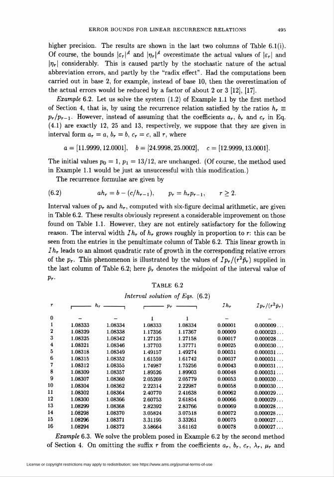
Example 6.2. Let us solve the system (1.2) of Example 1.1 by the first method

of Section 4, that is, by using the recurrence relation satisfied by the ratios hT =

Pr/pr-i- However, instead of assuming that the coefficients ar, bT and cr in Eq.

(4.1) are exactly 12, 25 and 13, respectively, we suppose that they are given in

interval form ar = a, br = b, cr = c, all r, where

a = [11.9999,12.0001], b = [24.9998,25.0002], c = [12.9999,13.0001].

The initial values p0 = 1, pi = 13/12, are unchanged. (Of course, the method used

in Example 1.1 would be just as unsuccessful with this modification.)

The recurrence formulae are given by

(6.2) ahr = b — (c/hr-i), Pr = hrPr-l, T>2.

Interval values of pr and hr, computed with six-figure decimal arithmetic, are given

in Table 6.2. These results obviously represent a considerable improvement on those

found on Table 1.1. However, they are not entirely satisfactory for the following

reason. The interval width Ihr of hr grows roughly in proportion to r: this can be

seen from the entries in the penultimate column of Table 6.2. This linear growth in

Ihr leads to an almost quadratic rate of growth in the corresponding relative errors

of the pr. This phenomenon is illustrated by the values of Ipr/(r2pr) supplied in

the last column of Table 6.2; here pr denotes the midpoint of the interval value of

Pr-

TABLE 6.2

01

2

34

5

67

89

10

11

12

13

14

15

16

1.08333

1.08329

1.083251.08321

1.08318

1.08315

1.083121.083091.083071.083041.083021.083001.082991.082981.082961.08294

1.083341.083381.083421.083461.08349

1.083521.08355

1.08357

1.083601.08362

1.08364

1.083661.08368

1.083701.083711.08372

Interval solution of Eqs. (6.2)

- Pr -.

11.08333

1.17356

1.271251.377031.49157

1.61559

1.74987

1.895262.052692.223142.407702.607532.82392

3.05824

3.311953.58664

1

1.08334

1.173671.27158

1.37771

1.49274

1.61742

1.75256

1.899032.057792.229872.416382.61854

2.837663.07518

3.332613.61162

Ihr

0.00001

0.000090.00017

0.000250.000310.000370.000430.000480.00053

0.000580.000620.000660.00069

0.000720.00075

0.00078

Ipr/(r2Pr)

0.000009.0.000023.0.000028.

0.000030.0.000031.0.000031.0.000031.

0.000031.0.000030.0.000030.0.000029.0.000029.0.000028.

0.000028.0.000027.

0.000027.

Example 6.3. We solve the problem posed in Example 6.2 by the second method

of Section 4. On omitting the suffix r from the coefficients ar, br, cr, XT, ptT and


496 F. W. J. OLVER

vr, we obtain the recurrence relations

(6.3) aur = vpT + pUr-l, Pr+i = Ur + XpT, T > 1,

in which

A = b/(2a), p = c/X, v = b — aX — p.

The initial member of the sequence {uT} is given by uo = Pi — Apo- Interval values

of A, p and v are found to be

A = [1.04164,1.04169], p = [12.4797,12.4803], v = [0.0196000,0.0204000],

and using six-figure decimal arithmetic we arrive at the interval values of pr and

ur displayed in Table 6.3.

For large r, the intervals containing pr are narrower than those obtained in Table

6.2 but from the last column, in which pr again denotes the mean value of pr, it is

evident that the growth of the relative error is still not linear in r.

Table 6.3

Interval solution of Eqs. (6.3)

T I- "r-1 i- Pr -, Ipr/(rpr)

01

2

34

567

89

10

11

12

13

14

15

16

I-

0.04164000.04507350.0487915

0.05281760.05717730.06189830.06701050.07254630.0785408

0.08503170.09206080.09967160.1079130.116838

0.126502

0.136967

-1

0.04170000.04521130.04901680.05314120.05761120.06245570.06770610.0733965

0.07956380.08624830.09349330.101346

0.109856

0.1190790.129076

0.139910

1.083331.173501.27115

1.376891.491391.61538

1.74965

1.895042.05248

2.22297

2.407592.60751

2.823993.05841

3.312263.58714

1.08334

1.17373

1.271691.377861.49293

1.61764

1.752791.89927

2.058032.230082.41656

2.61866

2.837703.07509

3.33238

3.61122

0.00000.

0.00009.

0.00014.0.00017.

0.00020.

0.00023.0.00025.0.00027.0.00030.0.00031.0.00033.0.00035.0.00037.0.00038.

0.00040.0.00041.

Example 6.4. We compute the absolute value of the Bessel function Yr(x) by

forward recurrence from the relation

(6.4) pr + l = (2r/x)pr - Pr-i-

We take x = 100 and the initial values

(6.5) pioo = -Fioo(lOO) = 0.166921 Pioi = - Vioi (100) = 0.200285 ...

Using six-decimal floating-point arithmetic, with chopping, we obtain the values pr

given in the second column of Table 6.4.

We shall compute both a posteriori and a priori error bounds by the methods

of Section 5. These computations are carried out in four-decimal floating-point

arithmetic with chopping. In the terminology of [12] this is the lower mode of

computation (£), and its associated wrp is **¡¿ = 10-3. For the computation of the

pr, the wrp is 7 = 10~5.



Both types of error bound require the evaluation of the bounds (5.19) for the

coefficients tj. The zeros of the local characteristic polynomial z2 — (2r/x)z + 1 are

given by

aT = (r/x) + {(r/x)2 - l}1'2, ßr = (r/x) - {(r/x)2 - l}1'2.

Consequently, for any n exceeding 100, we have

a = aioi = 1.15177... , B = ß101 = 0.868225... ;

compare (5.13). Also, from (5.17) and (6.5) we see that p = a. From (5.19) we

derive

(6.6) ¿loo < 3.061... ; t, < 4.061... , j > 101.

For simplicity, however, we use the same bound for all j:

(6.7) tj < 4.062, j > 100.

For a posteriori error bounds we need to compute bounds for the quantities 0r

defined by

Pr = {(2r- 2)/x}Pr-i - pr-2 +<t>r, T> 102;

compare (5.2). Since the coefficient (2r - 2)/x is exact, only two chopping errors

are introduced at each recurrence step. Applying the methods of [12] we find that

|0r| < Xrie3^, r>102,

where

Xr =Pr + {(2r-2)/x}pr-i,

and the double bar signifies the value computed in L. The rest of the computation

proceeds in accordance with the relations (5.21), (5.22) and (5.23), as described in

Section 5. The main steps are shown in columns 3, 4, 5 and 6 of Table 6.4: As in

Example 6.1, the superscripts A and S signify upper and lower bounds respectively.

Again, these bounds were computed using the methods of [12].

TABLE 6.4

Bessel function —Yr(x)

r Pr Xr 105Tf 105|er|" \er/pr\A eT/pr Â

0.000004... 0.000370.000007... 0.000600.000011... 0.00082

0.000013... 0.00104

0.000016... 0.00127

0.000021... 0.00149

0.000032... 0.001720.000048... 0.00194

0.000057... 0.00216

0.000063... 0.002390.000067... 0.002610.000074... 0.00284

0.000077... 0.003060.000084... 0.00328

0.000088... 0.003510.000090... 0.00373

0.000092... 0.00396

100

101

102

103104

105

106

107

108

109

110

111

112113

114

115

116

117

00

00

0

0

00

1

1

2

3

5

914

24

41

72

118 128

.166921200285.237654

.284529348475

440299

576152

781141

09548585083599960689

6473004301

7899677896906902126

0.6421

0.76930.93451.165

1.5002.002

2.766

3.9515.8148.797

13.6521.68

35.2158.3998.71

170.0

298.1

4.531

15.70

26.94

38.1449.20

60.1370.94

81.61

92.21102.7

113.1

123.5133.9

144.3154.6

164.8

175.1

0.23750.28440.34820.43990.5757

0.7805

1.094

1.5832.356

3.6015.6399.030

14.75

24.6341.8972.56

3.7557.710

13.3521.78

34.86

55.76

89.94147.0

243.8410.8

702.61218214738406966

12810

23920

0.000160.00028

0.000390.00050

0.00061

0.00072

0.000830.000930.001040.00114

0.00125

0.001350.00146

0.001560.001660.00177

0.00187


498 F. W. J. OLVER

By way of comparison, the seventh column of Table 6.4 gives an upper bound

\er/pr\A for the relative error. This is derived from the entries in the second and

sixth columns. The next column gives the value of the actual relative error er/pr

computed by use of high-precision values of Fr(100). Our bound overestimates the

true error by a factor that ranges from about 35 at the beginning of the recurrences

down to about 20 at r = 118. Two sources contribute to this factor. First, there is

the radix effect associated with base 10. As we observed in Example 6.1, use of base

2 instead might save a factor of about 2 or 3. Secondly, we have used a uniform

bound, given by (6.7), for the tj. In fact, most of these coefficients are considerably

less than 4.062. If desired, smaller bounds could be used without changing the

0(r) estimate of the total computing effort. For example, since the sequence ßr is

decreasing, it is easy to see that the second of the bounds (5.19) can be replaced

by

tj < a/(a - ßj), 101 <j<n.

The quantity a/(a - ßj) has the values 2.258... and 1.925 ... at j = 110 and 118,

respectively. Further sharpening is possible by application of the theorems given in

[6, Section 5].

The final column of Table 6.4 gives a priori bounds wA for the relative precision

of the approximation pr to pr. These were found as follows. Since the coefficients

in (6.4) are exact, we have 6 = 0. Also, since Cj-i = a¿_i, all j, and only two

chopping errors are made at each recurrence step, Eq. (5.24) may be replaced by

Wr = 2 \ (tioo + t101)nj + 7 ¿ t3 (2 + VjL± ) \, j> 102.

[ ,=102 V P>')

On taking cr; = 7 = 10~5, substituting for the tj by means of (6.6) and using the

fact that pj-2/pj < 1/p2, all j, we arrive at the numerical form

tcy < {14.25 + (22.40)(r - 101)} x 10-5, r > 102.

As expected, the values of vcA are approximately twice the size of the a posteriori

relative error bounds \er/pr\A■

7. Conclusions. We have described various methods for computing error bounds

for solutions of difference equations of the form

ClrPr+1 = bTPr + Crpr-1

that are generated by forward recurrence. Two cases are considered: (A) oscillatory

systems, in which b2-\-Aarcr < 0, all r; (B) monotonie systems, in which b2+iarcr >

0, all r. In Case B methods have been provided for finding bounds of both a

posteriori and a priori types. In Case A, only an a posteriori method is available,

and there is a need for a method for constructing a priori bounds analogous to that

of Section 5.

Acknowledgments. Helpful comments on this work have been made by J. R.

Cash, E. Kaucher and D. W. Lozier, and especially the referee. I am also pleased

to acknowledge the assistance of Dr. Lozier with the generation of high-precision

values of the Legendre and Bessel functions needed in Examples 6.1 and 6.4.



University of Maryland

Institute for Physical Science and Technology

College Park, Maryland 20742

National Bureau of Standards

Mathematical Analysis Division

Gaithersburg, Maryland 20899

1. J. R. CASH, Stable Recursions, Academic Press, London, 1979.

2. W. Gautschi, "Computational aspects of three-term recurrence relations," SIAM Rev., v.

9, 1967, pp. 24-82.

3. W. GAUTSCHI, "Zur Numerik rekurrenter Relationen," Computing, v. 9, 1972, pp. 107-

126. [Translated as Report ARL 73-0005, Aerospace Research Laboratories, Wright-Patterson Air

Force Base, Ohio, 1973.]

4. W. GAUTSCHI, "Computational methods in special functions—a survey," in Theory and

Application of Special Functions (R. A. Askey, ed.), Academic Press, New York, 1975, pp. 1-98.

5. N. J. HlGHAM, "Efficient algorithms for computing the condition number of a tridiagonal

matrix," SIAM J. Sei. Statist. Comput., v. 7, 1986, pp. 150-165.

6. R. M. M. MatTHEIJ, "Accurate estimates of solutions of second order recursions," Linear

Algebra Appl, v. 12, 1975, pp. 29-54.

7. R. M. M. MATTHEIJ & A. VAN DER Sluis, "Error estimates for Miller's algorithm," Numer.

Math., v. 26, 1976, pp. 61-78.

8. R. E. MOORE, Methods and Applications of Interval Analysis, Society for Industrial and Ap-

plied Mathematics, Philadelphia, 1979.

9. F. W. J. OLVER, "Error analysis of Miller's recurrence algorithm," Math. Comp., v. 18, 1964,

pp. 65-74.10. F. W. J. OLVER, "Numerical solution of second-order linear difference equations," J. Res.

Nat. Bur. Standards Sect. B, v. 71, 1967, pp. 111-129.

11. F. W. J. OLVER, "Bounds for the solutions of second-order linear difference equations," J.

Res. Nat. Bur. Standards Sect. B, v. 71, 1967, pp. 161-166.

12. F. W. J. OLVER, "Further developments of rp and ap error analysis, " IMA J. Numer. Anal.,

v. 2, 1982, pp. 249-274.

13. F. W. J. OLVER & J. H. WILKINSON, "A posteriori error bounds for Gaussian elimination,"

IMA J. Numer. Anal., v. 2, 1982, pp. 377-406.

14. S. M. RUMP, "Solving algebraic problems with high accuracy," in A New Approach to Sci-

entific Computation (U. W. Kulisch and W. L. Miranker, eds.), Academic Press, New York, 1983,

pp. 51-120.15. A. VAN DER SLUIS, "Estimating the solutions of slowly varying recursions," SIAM J. Math.

Anal., v. 7, 1976, pp. 662-695.

16. R. TAIT, "Error analysis of recurrence relations," Math. Comp., v. 21, 1967, pp. 629-638.

17. P. R. TURNER, "The distribution of leading significant digits," IMA J. Numer. Anal., v. 2,1982, pp. 407-412.

18. J. H. WILKINSON, Rounding Errors in Algebraic Processes, National Physical Laboratory

Notes on Applied Science No. 32, Her Majesty's Stationery Office, London, 1963.

19. J. WlMP, Computation with Recurrence Relations, Pitman, Boston, 1984.


Documents

Error Bounds for Linear Recurrence Relations*...1. Introduction. The application of mth order linear recurrence relations (1.1) ar0Pr + arlPr-l + ar2pr-2 -\-h OrmPr-m + dr = 0, in