Error Analysis Booklet - Jacobs University · PDF fileError analysis booklet 1. ... K. F. Riley, M.P. Hobson, S.J. Bence: Mathematical Methods for ... cuit to deposit 0.0011180 grams

Natural Science and Advanced

Laboratories in Physics

Error Analysis Booklet

forPhysics Teaching Labs

at

Jacobs University

Summary of error analysis based on standard textbooks and instruction manuals forphysics lab courses. Natural Science and Advanced Physics Labcourses, Jacobs UniversityBremen, 1st Edition, Fall 2010, Prof. Dr. Jurgen Fritz and Frank RosenkotterAugust 2011 corrected and extended Version, Version F11 - P01,

Contents

1. Introduction . . . . . . . . . . . . . . . . . . . . . . . . . . . . . . . . . . 11.1 Definition and classification of errors . . . . . . . . . . . . . . . . . . . . . 2

2. Directly measured quantities - mean value and standard deviation 52.1 Additional Note for advanced analysis . . . . . . . . . . . . . . . . . . . . 72.2 Derivation of the formula for the mean value . . . . . . . . . . . . . . . . . 8

3. Reporting and presenting results from error calculation - signifi-cant digits . . . . . . . . . . . . . . . . . . . . . . . . . . . . . . . . . . 10

4. Indirectly measured quantities - error propagation . . . . . . . . . . 114.1 Explanation of error propagation theorem . . . . . . . . . . . . . . . . . . 124.2 Comparing and evaluating errors . . . . . . . . . . . . . . . . . . . . . . . 14

5. Analysis of straight line functions . . . . . . . . . . . . . . . . . . . . 155.1 Graphical determination of slope and intercept . . . . . . . . . . . . . . . . 165.2 Mathematical determination of slope and intercept . . . . . . . . . . . . . 165.3 Line through the origin . . . . . . . . . . . . . . . . . . . . . . . . . . . . . 18

6. Appendix . . . . . . . . . . . . . . . . . . . . . . . . . . . . . . . . . . . . 196.1 Summarized Procedure of Error Calculation . . . . . . . . . . . . . . . . . 196.2 Gaussian Distribution . . . . . . . . . . . . . . . . . . . . . . . . . . . . . 20

Error analysis booklet

1. Introduction

The success of natural sciences is based on a strong and dynamic interaction betweentheory and experiment. Every theory has to be proven by experiments, and vice versanew theories might provide inspiration for new experiments. Without doubt, this inter-play is only possible if experiments are carried out as precise and reliable as possible. Theknowledge of the reliability of a measured value is therefore of fundamental importancein science and technology. Theories in physics might be accepted or not depending onthe fit of experimental values to a predicted theoretical range.Examples of applied error analysis in modern industry and technology are that manymachines are assembled by parts from different countries, and engineers have to agree oncertain error margins for their parts, so that e.g. a screw from China properly fits intoa nut from Sweden. But also in athletics, for example, it is important to know aboutcalibration of instruments and uncertainties of measurements to be able to judge if e.g.a time measured for a run is faster compared to the recent world record. For scientistsand engineers it is therefore essential to have a detailed understanding and experienceon how uncertainties in a measurement can be identified, quantified, and reported. Indoing so, one can also identify potential sources of errors so that they can be reduced oreven be avoided. It certainly has been and will be one of the driving forces of scienceand technology that scientists always want to know values as exact as possible, and notbeing satisfied with vague answers or a wide spread of experimental results.

Although the methods of error analysis need a thorough mathematical knowledge, forpractical purposes the application of a few formulae and procedures is often sufficient.Therefore, the most important facts for error analysis in physics-related sciences are sum-marized in this booklet. Additional mathematical derivations of formulae and books forfurther reading are given as additional information. The following four books, which alsohave been used to prepare the booklet, are recommended for an in-depth study on erroranalysis and statistics:

Guide to the Expression of Uncertainty in Measurement (GUM), JCGM (2008, corrected2010). International standard guide for industry on measurements produced by the JointCommittee for the Guides in Metrology (including the Bureau International des Poids etMeasures, Paris).John R. Taylor: An Introduction to Error Analysis, Univ. Science Books, 2nd ed. (1997).This is the classical book on error analysis with a very thorough and understandablemathematical background.G. L. Squires: Practical Physics, Cambridge Univ. Press, 4th ed. (2001). This book hasless mathematical background but in addition some information on experimental designand report writing.K. F. Riley, M.P. Hobson, S.J. Bence: Mathematical Methods for Physics and Engi-neering, Cambridge Univ. Press, 3rd ed. (2006). The last two chapters deal with themathematical background of probability and statistics.

In the first part of this booklet properties and notation of different types of errors aregiven. Afterwards, the handling of random errors is explained with respect to their sta-tistical properties. This is followed by how errors from different values contribute to afinal calculated value. Finally, some information on data fitting is given.

–1 – Jacobs UniversityAugust 2011, Version F11 - P01


1.1 Definition and classification of errors

The word error is a bit misleading since error analysis is not concerned with a ”mistake”or ”failure” of something. Error analysis allows to calculate a data range, where the “truevalue”, i.e. the most reliable or best value, of a measurement can be expected. Therefore,the word uncertainty is sometimes preferred over ”error”. For a better understandingfirst some of the basic expressions in error analysis will be defined.

There is no measured true value of a specific quantity in a philosophical sense, only themost accepted value or a defined standard value is defined as ”true”. Different methodsof measuring the same quantity usually give slightly different answers or values. Thereis a great deal of effort put into developing accepted values for certain properties so thatscientists can calibrate their instruments before going to measure unknown quantities.Even standards change occasionally, when the situation warrants revision. For example,until 1948 the Coulomb was defined as the quantity of electricity passing through a cir-cuit to deposit 0.0011180 grams of silver from a solution of silver nitrate. Nowadays,the Coulomb is defined as the quantity of electricity on the positive plate of a 1 Faradcapacitor subject to an electromotive force of one Volt. Thus it makes sense to define areasonable true value for theoretical considerations.Uncertainty is a notation for the range around the measured most reliable value theexperimenter expects the true value to be within (with a certain propability). It is ameasure of possible deviations from the true value which can be in positive or negativedirection.Deviation describes the discrepancy of a result from the expected value. Do not mixdeviation with uncertainty of a result!Accuracy is a measure of the agreement of a particular measurement with the true oraccepted value. In principle, the accuracy is a systematic deviation which can have apositive or negative sign. A measure of the accuracy can only be determined if someprior knowledge of the true value is available. The accuracy becomes important if thecalibration of an instrument changes with environmental parameters such as e.g. tem-perature. In this case, the manufacturer gives an accuracy of the instrument valid in acertain temperature range. This accuracy has to be taken as additional deviation for theuncertainty of the measurement.Precision describes the variability of a parameter for repeated measurements. In otherwords, it is defined as the degree of agreement between replicated measurements of thesame quantity. The resulting values might vary randomly between different measure-ments. The difference between accuracy and precision is illustrated in Fig.1-1

Errors in general can be separated in two major classes which show different characteris-tics in terms of their sources, how they can be identified, and how they can be reduced:Random errors arise from natural or random fluctuations (e.g. thermal noise). Theyfollow statistical, random principles and are bidirectional, that is, they are equally dis-tributed (in a Gaussian distribution) around a mean value. Most importantly, they arealways present, cannot be avoided, but can be reduced by repetitive measurements. Ran-dom errors can be quantified by a statistical description. There are two more subtypesof random errors. ”Instrumental errors” are uncertainties of scientific instruments pro-

2 ,

Physics Teaching Lab

Figure 1-1: Differences between accuracy and precision.

vided by their manufacturer. They indicate how precise a measurement can be or whatspread of values you can expect when measuring the identical experimental parametermany times. With this respect they fall into the category of random errors. Anothertype of error is kind-of random but cannot be treated by statistical means. These are”accidental” errors, which are caused for example by an accidental kick against the labtable, an occasional guest of wind, or switching on the light in a dark room experiment.These events appear random but they are singular events due to a known disturbance ofthe setup, and they have to be avoided in any reliable experiment. Values obtained fromsuch situations are normally excluded from the experimental data (the experiment needsto be repeated), but nevertheless, they can be used to produce worst case scenarios for anexperimental setup to get an idea on its robustness or sensitivity to external influences.Systematic errors can also be called ”experimental mistakes”. They can arise fromthe use of a wrong experimental method, a wrong instrumental calibration, from uncon-trolled environmental conditions (e.g. changes in room temperature), or from a biasedselection of experimental data. They result in an unidirectional offset of results from theexpected value and might be identified by rechecking the theory, changing experimentalmethods or conditions. They are sometimes hard to identify but one certainly has toeliminate all possible systematic errors to get reliable results. Part of getting an excellentexperimental scientist is to be always suspicious against hidden systematic errors in anexperiment, then recognize and correct them.

The time taking during a 100 m run is a good example to illustrate both types of errors.Before the introduction of the electrical time taking, several timekeepers with manualstopwatches have stopped the time as follows: The stopwatch was started with the ap-pearance of the cloud of smoke from the starting signal pistol and was stopped as soon asthe runner crossed the finish line. The watches of 5 different timekeepers showed timesdiffering by 0.1 to 0.2 sec. These different times were assumed to be randomly distributed,and their average was calculated and taken as actual result. Then for a certain periodin the past, the time was stopped by hand and at the same time electrically (to 1/1000sec): firing the starting pistol directly starts an electronic watch until the photo finishcamera takes the time of the runner crossing the finish line. In doing so the electricallystopped time was systematically longer by approximately 0.1 sec. This difference cannotresult from the different precisions of the stopwatches and the electrical watch. But whenanalyzing the measuring procedure for the 100 m run it became clear that a timekeeper

Jacobs University, August 2011, Version F11 - P01 3


has a short reaction time until he starts the stopwatch: he waits until he sees the cloudof smoke coming out of the pistol, then reacts and presses the stopwatch. On the otherhand, he has basically no time delay when the runner crosses the finish line since heanticipates in advance when the runner will cross the line. Therefore, the time stoppedby hand must be systematically shorter than the real time the runners are on their way,whereas the electrical measurement comes up to the real value with a negligible reactiontime.Another example of a systematic error is measuring a distance with a steel measuringtape: The measuring tape is calibrated for a certain temperature (e.g. 25◦C). If the mea-suring tape is used at another temperature this leads to systematic errors, which can, atleast in principle, be corrected.

In a well designed experiment the identified systematic error sources can be reduced oreven eliminated. For both, lab course experiments and research, a proper error analysisincludes always a check, whether any systematic error might be present in the chosenset-up. If there might be a systematic error you cannot correct for, it is important toestimate its influence on the result and to compare its magnitude to the random errors(uncertainties). The deviation due to systematic errors has to be kept smaller or in thesame order than the uncertainty from random errors. If necessary, the experiment has tobe repeated with a more appropiate setup. For applying the formulas of calculation ofrandom errors one acctually assumes that no systematic error is present, since they arein principle avoidable.

Errors can be reported as absolute or relative errors. Whereas an absolute errorof ± 0.1 m for a best value of 1.0 m describes a poor measurement, the same error of± 0.1 m on a distance of 100.0 m is a precise measurement. To estimate the quality of ameasurement absolute errors have to be reported together with their best values. Abso-lute errors have always to be given with their correct units. The fractional uncertaintyor relative error indicates the quality of a measurement whatever the size of the bestvalue is. The relative error is defined as the ratio of absolute error to best value and istypically given in percent without units.A very simple rule of thumb is that typical experimental errors are around 5%. If theyare higher than 10% you really should re-evaluate your method or procedure to improveits reliability. If errors are smaller than 1% you have to prove in more detail that yourmeasurement is indeed such precise.In the following, the main principles for analyzing random errors are presented. Allformulae are based on statistics as the theoretical background for error analysis. All sys-tematic errors are neglected. We start with the determination of errors of a directly andrepetetively measured quantity. Afterwards, the error propagation theorem is presentedwhich describes the calculation of the error of a quantity that is calculated from severalother quantities which all have a certain uncertainty.

4 ,


2. Directly measured quantities - mean value and standard de-viation

The best way to quantify unavoidable random errors is to perform repetitive measure-ments. According to statistics, we can assume that the measured values are randomlydistributed around their true value forming a Gaussian distribution, i.e most values ac-cumulated near the true value. This set of data points is then used to determine thebest or most reliable value including an estimation of its error.If a quantity x is measured n times the best value representing the measurement is theaverage or arithmetic mean value x:

x =1

n·

n∑i=1

xi (1-1)

To describe how reliable a mean value is, one has to determine the error of the mean. Theerror of the mean value, i.e. the quality of the averaged result, depends on the numberof measurements and on the averaged deviations of individual measurements from themean value. The latter is illustrated in Fig. 1-2. It is quite clear that series b) is a more

Figure 1-2: Measurement of x with different precisions.

precise measurement than a) because the individual test points are closer to x assumingthe same number of measurements and the same scale for the x-axis in both cases.To calculate the error of the mean one has to determine first the averaged deviation ofall measured values from the mean. Since positive and negative deviations would cancelone uses the averaged root mean square of the deviations. The resulting value is calledthe population standard deviation σx (its squared value σ2

x is called the variance):

σx =

√√√√ 1

n

n∑i=1

(xi − x)2 (1-2)

The standard deviation σ of the individual measurement thus provides a value expressinghow much on average an individual value xi of a series of measurements deviates fromthe mean value x.But not all measured values fall within a range |xi − x| < σx from the mean value, only acertain percentage. We can also quantify the probability with which a single measurementwill fall within the standard deviation around the mean value. In case the distribution of



deviations dxi = xi − x follows the Gaussian distribution (as defined above for randomerrors), the standard deviation gives an information about the probability P (k) for ameasured value of x to be within the range x± k · σx. Since the Gaussian distribution isa non-linear function, the probability P (k) to find a measured value in the given rangeincreases drastically for k = 2 or 3 compared to k = 1 as given in Table 1-1:The statement that a measured value is with 68% probability within the standard devia-

k 1 2 3

Fractional probability P (k) 0.68 0.95 0.997

Table 1-1: Fractional Probability P (k) is the probability for a measured value x to bewithin the range of x± k · σx,n−1.

tion around the averaged value can also be rephrased as: If you do a single measurement,the probability is 68% that your result will be within the standard deviation around thetrue value. However, you have to keep in mind that about 1 out of 3 measured values isnot within the above mentioned interval.An important feature of the standard deviation is that it converges to a single value forincreasing n and it stays constant when the number of measurements tends towards infin-ity (for a perfect Gaussian distribution). Thus, the standard deviation is the parameterused to describe the precision of a measurement or the range in which 2/3 of data pointscan be found.In contrast to the population standard deviation in formula (1-2), which underestimatesthe uncertainty for a low number of measurements, there is a more commonly used defi-nition of the standard deviation:

σx =

√√√√ 1

(n− 1)

n∑i=1

(xi − x)2 (1-3)

It is the sample standard deviation. You might check that for n = 1 formula (1-2)gives an uncertainty of zero, whereas formula (1-3) results in an undefined standard devi-ation (divison by sero) which makes more sense for a single measurement, since for thatone can not define an error.One can also say that using the denominator n−1, the population standard deviation ex-presses the probability for the true value to be in the given range. Using the denominatorn, the sample standard deviation determines the probability for the next measurementto be within the given range. The difference between (1-2) and (1-3) is almost alwaysinsignificant and one should normally use formula (1-3) for calculations. In case of doubt,you should indicate which standard deviation and which denominator has been used toavoid misunderstandings.

What one finally reports as uncertainty of an experimental result is the averaged error of

6 ,


the mean ∆x (sometimes also called standard error of the mean) which is given by:

∆x =σx√n

=

√√√√ 1

n(n− 1)

n∑i=1

(xi − x)2 (1-4)

The error ∆x decreases inversely proportional to√

n. The justification of the√

n in thedenominator can be done via error propagation (see the book of Taylor). Formula (1-4)tells you the more measurements you do, the smaller your experimental error. But thenumber of measurements has to be increased e.g.by a factor of 4 to reduce the error of theaveraged value from an experiment by a factor of 2. The best or ”true” value is withinthe range of the confidence interval x±k ·∆x with the probability of P(k) as determinedin Table 1-1. The fractional probability (see Table 1-1) is also called confidence level.Without additional notes one assumes that an error indicates a σ or 68% confidence level.Different definitions or higher confidence levels have to be clearly identified.

2.1 Additional Note for advanced analysis:

0 5 10 15 20 25 30 35 40 45 500.0

0.1

0.2

0.3

0.4

0.5

0.6

0.7

0.8

0.9

Rel

ativ

e un

certa

inty

of σ

number of measurements n

20% - n=13

10% - n=51

36% - n=5

Figure 1-3: Relative uncertainty of the sample standard variation σ as a function of thenumber of measurements.

Obviously the sample standard deviation is the best approximation for the populationstandard deviation with the number of measurements n → ∞. However, due to its



statistical nature, σx of a Gaussian distribution has by itself a relative uncertainty ∆σx

σx

of 1/(2n− 2)12 , which is shown in Fig. 1-3. The uncertainty in σ depends strongly on the

number of data points. For three data points this uncertainty amounts to 50%, indicatinga very high uncertainty of the measurement itself. The value decreases only very slowly:For five data points the deviation is still 36%. To have an uncertainty of less than 20% oreven 10%, the number of data points has to be higher than 13 or 51, respectively. Thismight be taken as a general warning that for a meaningful experimental evidence onehas to perform a reasonable number of measurements and not only one or two.The problem of statistics of a low number of measurements has already been tackled atthe beginning of the 20th century. Helmert and Luroth have first derived a mathematicalsolution of this problem, resulting in the so-called t-distribution, which is a modifiedGaussian distribution. In 1908 William Sealy Gosset published a work in a journal underthe pseudonym ”Student”, that is also used as another name of the t-distribution. Due

0 10 20 30 40 500

1

2

3

4

5

6

99.7 %

95 %k S

tude

nt

number of measurements n

68 %

Figure 1-4: Value for k determining the confidence interval x ± k · ∆x for the Gaus-sian (lines) and the Student t-distribution (symbols) in dependence of the number ofmeasurements.

to the low number of measurements the uncertainty in the mean value x is larger thanexpected from the Gaussian distribution. Therefore, the averaged error of the meanhas to be corrected for the applied confidence level. The dependence of this correctionfactor k from the number of measurements can be found in Fig. 1-4. For more than 13measurements the value of k of the Student distribution converges towards the value ofthe Gaussian, whereas for the higher levels even more measurements are needed.

8 ,


2.2 Derivation of the formula for the mean value

If a quantity X is measured n times the result can be displayed as given in Fig. 1-5. Eachvalue is indicated by i from 1 to n.

In an illustrative form we would take as “best value” X the one showing the same

Figure 1-5: Display of different measurement values xi of quantity X.

deviations of xi of X from top to bottom. If all distances dxi = (xi −X) from the singlemeasurement value xi to the mean value are summed up, the sum equals to zero.

n∑i=1

dxi =n∑

i=1

(xi −X) = 0 (1-5)

n∑i=1

xi − n ·X = 0

X =1

n

n∑i=1

xi (1-6)

Which is the definition of the mean value from equation 1-1.Assuming an unknown value X ′ as good value and the error dxi = xi −X ′ is a functionof the value X ′. The quantity

Q =n∑

i=1

dx2i

is then minimal for the best value of X ′best. The minimum of Q results from

dQ

dX ′ = 0

That means:

d∑

(dx2i )

dX ′ =d

∑(xi −X ′)2

dX ′ = 0

⇔ − 2n∑

i=1

(xi −X ′best) = 0

⇔ nX ′best =

n∑i=1

xi ⇔ X ′best =

1

n

n∑i=1

xi = X



In conclusion we can say: The “best value”, i.e. the mean value X, results from theminimization of the squared absolute deviations.

3. Reporting and presenting results from error calculation - sig-nificant digits

After calculating the best value (that is the mean value) and the reliability of the bestvalue (that is the error of the mean) for an experimental outcome, the resulting quantitieshave to be presented in a scientific way. By calculating a mean value by a calculator oranalysis program the display might show e.g. a 10 digit number, and one has to thinkif all digits are indeed useful. Certainly not! Just reporting all digits from a numericalcalculation is in most of the cases simply wrong since it indicates a precision of a mea-surement which cannot be supported by experimental evidence.When reporting a single value (e.g. from a textbook or table) without an explicit error,one normally assumes that all digits are correct except the last digit which might berounded or is uncertain relating to the state-of-art of the measurement. How then reportyour calculated value? You first have to determine the error of your measurement, thenyou can adjust the precision of your best value to the error you determined. Lets assumeyou calculated a mean value of 346.47 m and an error of the mean of 1.21738 m. Itcertainly does not make sense to report all digits (or figures) of the error value, becauseif there is already an uncertainty of ± 1.3 in your measurement, no one cares if there ise.g. an additional one thousands part more or less uncertainty. The basic rule for that is:An error value must not be given with more than two significant digits! Youmight have realized that the uncertainty in the example above is given as ± 1.3 and not± 1.2 . This is another rule saying that errors are always rounded up!To report an error correctly, we first have to define what significant digits are: Signif-icant digits (or sometimes also called significant figures) are defined as the figures of anumber which give an information about the number. The following rules apply for thedetermination of significant digits:

1. The non-zero-digit most on the left is the most significant digit, e.g. the figure’1’ in 0.001230

2. The least significant digit is given

for figures without digital point by non-zero-digit most on the right, e.g. thefigure ’4’ in 271340

for figures with decimal point by the digit most on the right, e.g. the figure’0’ in 2.71340 · 105.

3. All digits from the most to the least significant digit are significant digits, e.g.0.001230 has four significant digits.

Finally, when one has determined the error of a measurement with two significant digits,then the result of the measurement, the best value, has to be adjusted to the precision(same order of magnitude of least significant digit) of the error value. In our example

10 ,


when the result is calculated as 346.47 m and the error was determined as ±1.3 m, thenthe final results will be (346.5 ± 1.3) m. Remember that results from an experimentshould always be reported as numerical values together with the correct units. Thenumerical value should contain the best value of the experiment together with its uncer-tainty range.Remarks: here the best value was rounded according to the standard rule: roundingdown for digits below 5, rounding up for digit 5 and higher. The result could have also bereported as 346 m ± 2 m. Another remark: Round always from the original value onlyusing the next digit to the right. Do not round by using more digits to the right or byrounding the value digit by digit starting from the last digit: 346.47 is rounded correctlywith 4 digits as 346.5 or with three digits as 346, but not as 347.

4. Indirectly measured quantities - error propagation

Up to now we have calculated the mean value x and the standard deviation σx of a setof repetitive direct measurements of a single quantity xi. We do not know yet how anerror of a single quantity xi influences the error of another quantity calculated from xi.Or in other words, how does one determine the error of a quantity which is calculatedfrom several other quantities each of which has its own uncertainty? For example, whatis the error of the volume of a cylinder given different means and errors for its radius andheight?We assume the quantity y is a function of p parameters x1, x2, . . . , xp with

y = f(x1, . . . , xp) (1-7)

The error ∆y of y is calculated by the error propagation theorem. The derivation isgiven below.In theory, the deviation of a result from the expected value can be affected by each pa-rameter in the same direction. That means, that all partial changes of y due to deviationsin xi add up. In this case, the maximal error ∆ymax is given by:

∆ymax =

∣∣∣∣∣(

∂y

∂x1

)

xj 6=x1

∆x1

∣∣∣∣∣ +

∣∣∣∣∣(

∂y

∂x2

)

xj 6=x2

∆x2

∣∣∣∣∣ + . . . +

∣∣∣∣∣(

∂y

∂xp

)

xj 6=xp

∆xp

∣∣∣∣∣

=∑q=1

∣∣∣∣∣(

∂y

∂xq

)

xj 6=xq

∆xq

∣∣∣∣∣ Maximal Error (1-8)

However, since all parameters are assumed to be independent from each other, it is quiteunusual that all uncertainties of the directly measured values affect the mean value inthe same direction.Therefore, the error ∆y of the averaged value y is given by the averaged error, which is



the most often used error:

∆yavg =

√√√√[(

∂y

∂x1

)

xj 6=x1

∆x1

]2

+

[(∂y

∂x2

)

xj 6=x2

∆x2

]2

+ . . . +

[(∂y

∂xp

)

xj 6=xp

∆xp

]2

=

√√√√∑q=1

[(∂y

∂xq

)

xj 6=xq

∆xq

]2

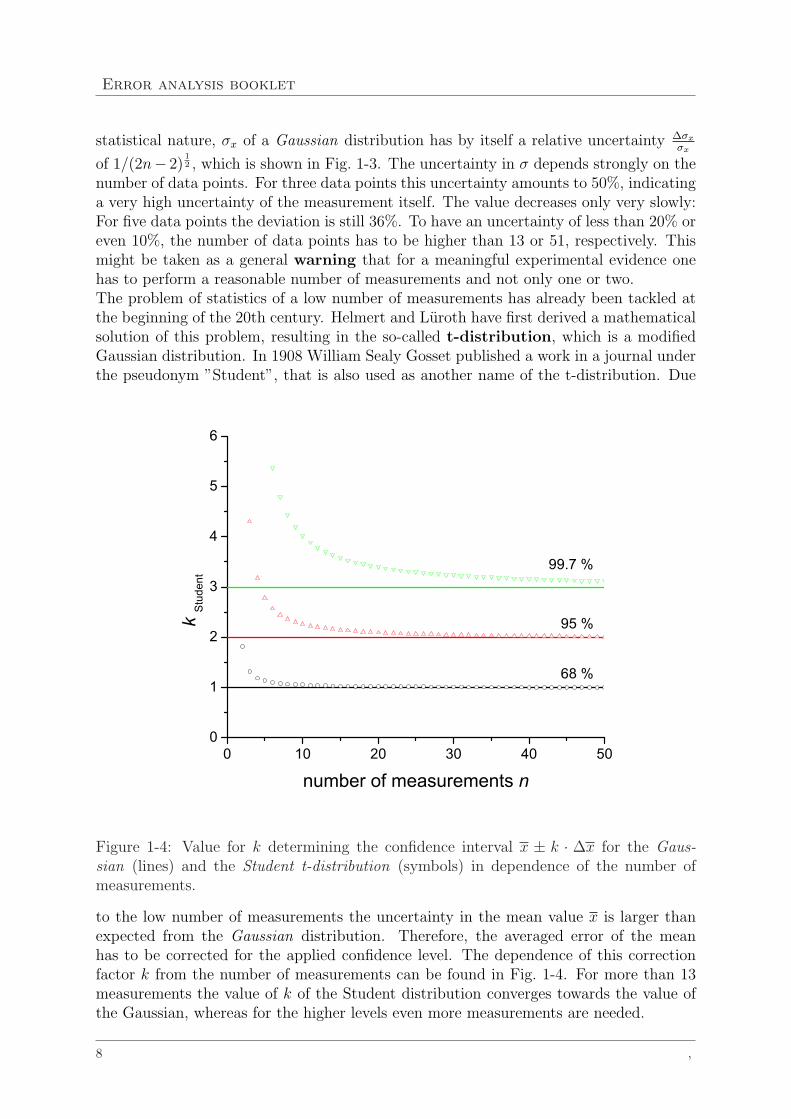
Averaged Error (1-9)

Note:There are two simplified rules for the propagation of errors that you should knowby heart since they can be used for most of the error calculations:

For sums and differences, the absolute errors add up.

For multiplication and division, the relative errors add up.

You either can add up errors directly to get the maximal error or can build thesquare root of the sum of the squared values for the averaged error.

Assuming the quantity y is a simple function of a and b only (where a and b are indepen-dent (!) variables), the rules described above are mathematically expressed as follows:

y = a + b =⇒∆ymax = ∆a + ∆b and ∆yavg =

√(∆a)2 + (∆b)2

y = a− b =⇒

y = a · b =⇒∆ymax

y=

∣∣∣∣∆a

a

∣∣∣∣ +

∣∣∣∣∆b

b

∣∣∣∣ and∆yavg

y=

√(∆a

a

)2

+

(∆b

b

)2

y =a

b=⇒

You can derive these rules if you apply the general error propagation formula to the givenfunctions. Attention: You cannot use this rule for e.g. y = x3 = x · x · x since the x’sin this formula are not independent! Instead you have to use the full error propagationformula and calculating the derivative of y with respect to x (solution ∆yavg = 3 ·x2 ·∆x.)

4.1 Explanation of error propagation theorem

Again, this paragraph gives more background on error propagation but it can be skippedfor a quick reading. As above we want to calculate the error of a quantity which is a

12 ,


function of one or more quantities which are determined with a limited precision. Theerror of the result is then calculated by error propagation.Assume the result y is calculated from different parameters xi. The effect of an error inxi on y will be derived from a special example: A machine produces many (n) apparentlyequal cylinders with a base of A = πr2 and a height h. We measure very exactly theradius r and the height h of every cylinder with a micrometer and state (of course) thatnot all cylinders have the same height h resp. radius r. r and h have a variance. Nowwe would like to know what effect this variance of r and h has on a composed quantity,i.e. the volume V = f(r, h) = πr2h. The averaged volume V results in:

V = πr2 · h

where r and h are the mean values each of set of values of ri and hi.The dependence of the volumes Vi on ri for a constant height h is displayed in Fig. 1-6and two exemplary results V1 and V2 are indicated by the continuous lines. The dashedlines illustrate the effect in the uncertainty range of V1 and V2 due the same uncertainty∆r. It does not matter whether ∆r corresponds to a standard deviation given by a set of

Figure 1-6: Illustration of the dependence of V and dV on r and dr.

different c ylinders or to an uncertainty due a single measurement with a finite precision.Again, to facilitate the reading, the notation ”error” is commonly used for both cases.As can easily be seen, the same error ∆r causes for r1 a much smaller error ∆V in V1

than for r2 in V2. In case of small changes, which shall be indicated by lower case “d”instead of “∆”, the calculation of change of volume dV due to a change in r of dr isillustrated in the right part of Fig. 1-6. In this case, the change dV can be assumed tobe linearly dependent on dr and is illustrated by the tangent in point ri. The change ofV in r due to dr is then given by the product of the slope of the tangent and dr.For error calculation, we need a mathematical method to calculate the slope. Assumingthat the change in r is infinitesimal small, the slope of the tangent is given by the



derivative of V with respect to r. In the given case, where V depends on the two variablesr and h the partial differential has to be used:

dV (r) =

(∂V

∂r

)

h

dr

A partial differential just expresses that V depends not alone on the parameter r. Thesubscript h denotes that the partial derivative of V with respect of r is calculated withthe assumption that h is constant. For application, this means that the partial derivativeis calculated as if V would depend only on r and the actual value of h is plugged into theformula.For the total change in V due to both dr and dh the total differential has to be derived.The total differential is the sum of the partial differentials with respect to h and r,respectively:

dV =

(∂V

∂r

)

h

dr +

(∂V

∂h

)

r

dh

For error calculation, the infinitesimal small changes in r and h are replaced by thediscrete errors ∆r and ∆h:

∆V =

∣∣∣∣(

∂V

∂r

)

h

∆r

∣∣∣∣ +

∣∣∣∣(

∂V

∂h

)

r

∆h

∣∣∣∣

Note that the absolute values have to be added to avoid that the different summandsmay cancel out each other.The slope of the tangent might not be representative for the change of volume in thecomplete range but the approximation is sufficiently good for error calculation.The previous formula gives ∆V assuming that both errors ∆r and ∆h tend to effect thevolume in the same direction. According to statistic law’s this is quite unusual and forindependent parameters r and h the error ∆V can be calculated by:

∆V =

√{(∂V

∂r

)

h

∆r

}2

+

{(∂V

∂h

)

r

∆h

}2

Generalized, the error ∆y of the composed quantity y = f(x1, . . . , xp) is given by theerror propagation theorem.As a further simplified rule in error propagation one can assume that the final resultcannot have more significant digits than the lowest number of significant digits of theinput values.

4.2 Comparing and evaluating errors

After having determined all errors (statistical analysis of random errors, instrumentalerrors and uncertainties of literature values, propagated error) the different results haveto be carefully evaluated and compared: maybe the statistical error is much smallerthan the instrumental error; or what is the most dominating error which needs to be

14 ,


reduced to get more reliable results? If you determined a statistical error from repetitivemeasurements and you have a given instrumental error, you should report them bothand compare them. Ideally, an experimental method should be such precise that the(calculated propagated) instrumental errors are smaller compared to the statistical errorsfrom repetitive measurements. In this case it is normally enough to report the statisticalerror and just mention the instrumental error. But especially in cases where you haveonly limited experimental data, the statistical error can be quiet small, or even be zero,and can therefore be much smaller than the instrumental error. In such a case you haveto judge if a small statistical error is indeed an indication for a precise experiment or ifit is just an artifact. Here an example: You measured five times an identical electricalcurrent of 1.0 mA. This could hint either for a real precise measurement, but it could alsoindicate a very crude measurement which measures the electrical current only in intervalsof 0.5 mA. Then values of 1.1 mA, 1.3 mA, or 1.4 mA all give a value of 1.0 mA as anoutput of your instrument. This would result in a statistical error of 0 indicating a veryprecise measurement, even when the individual (true) values deviate by several 10%. Inthis case it is important to report the instrumental uncertainty, which is about 50% inthis measurement, and use it for the interpretation of the reliability of the data (as aconsequence you should invest some more money for a more precise ampere meter).For a proper error analysis, errors should also be ranked as major and dominating errors,or minor and negligible errors to give an idea which are the least reliable input parametersof an experiment. To do so one has to have a look at the values of the summands underthe square root for the propagated error (Formula 1-9). For improving the experimentone has to work first on the experimental parameter producing the largest contribution tothe propagated error or on instrumental errors which are much larger than the statisticalerrors.

5. Analysis of straight line functions

In the previous section we assumed that identical measurements of one or more quanti-ties were repeated many times from which we derived their mean values and their errors.When plugging in these quantities in a formula we can also calculate the mean and errorof a final calculated value by error propagation. In another type of experiment one is in-terested in the mathematical relation between two quantities. To do so, one continuouslyvaries one quantity and observes the change of another quantity, for example one slowlyincreases the temperature T of a gas and at the same time measures its volume V . Fromthat data, a graph or curve V (T ) can be created and we now want to quantify also theerrors of the parameters of this curve.The most simple and most important example of such a function y(x) is a straight line.The case of a straight line is especially important, because a large set of “more com-plicated” curves like e.g. parabola, power, exponential, logarithm, hyperbola can betransformed to straight lines by appropriate transformation of the plot coordinates. E.g.f(x) = a em x appears as a straight line with slope m in a plot of log(f(x)) versus xor a parabolic dependence can be transformed to a straight line when plotting y vs x2.Straight line behaviour is most easily detected by visual inspection of a graph and a devi-ation from such a linear behavior (= straight line) is much easier to detect than deviationfrom potential, exponential, of logarithmic curve shapes. The procedure to find a straight



line which best fits the experimental data is called a straight line fit or linear regression,and will be explained below.If a quantity y is linearly dependent on the quantity x, the plot of y versus x describes astraight line. In general, a straight line function is completely described by the slopem and intercept c as given by equation 1-10:

y = mx + c (1-10)

m or c can then be easily determined by the measurement of y in dependence on x usinga graphical or mathematical method as explained in the following.

5.1 Graphical determination of slope and intercept

We first start with a ”manual” determination of the straight line and its errors. Fig. 1-7illustrates the graphical determination of slope and intercept including uncertainty.After plotting all data points including uncertainty bars (here only in y), two lines are

Figure 1-7: Graphical determination of slope and intercept including uncertainty.

drawn with the minimal and maximal possible slope. It is important that both linescontain or cross the uncertainty ranges of all data points. It is a common mistake whenapplying this method, that only the first and last data point with their error ranges aretaken into account.Afterwards, the different slopes mmin and mmax as well as the different intercepts cmin

and cmax of the resulting lines can be determined and a mean slope and mean intercepttogether with their errors can be calculated. m and c are then given by:

m =mmax + mmin

2∆m =

mmax −mmin

2(1-11)

c =cmax + cmin

2∆c =

cmax − cmin

2(1-12)

5.2 Mathematical determination of slope and intercept

Data sets resulting from experiments are usually more or less “noisy” as a result of ran-dom fluctuations of experimental parameters. Hence mathematical optimization methods

16 ,


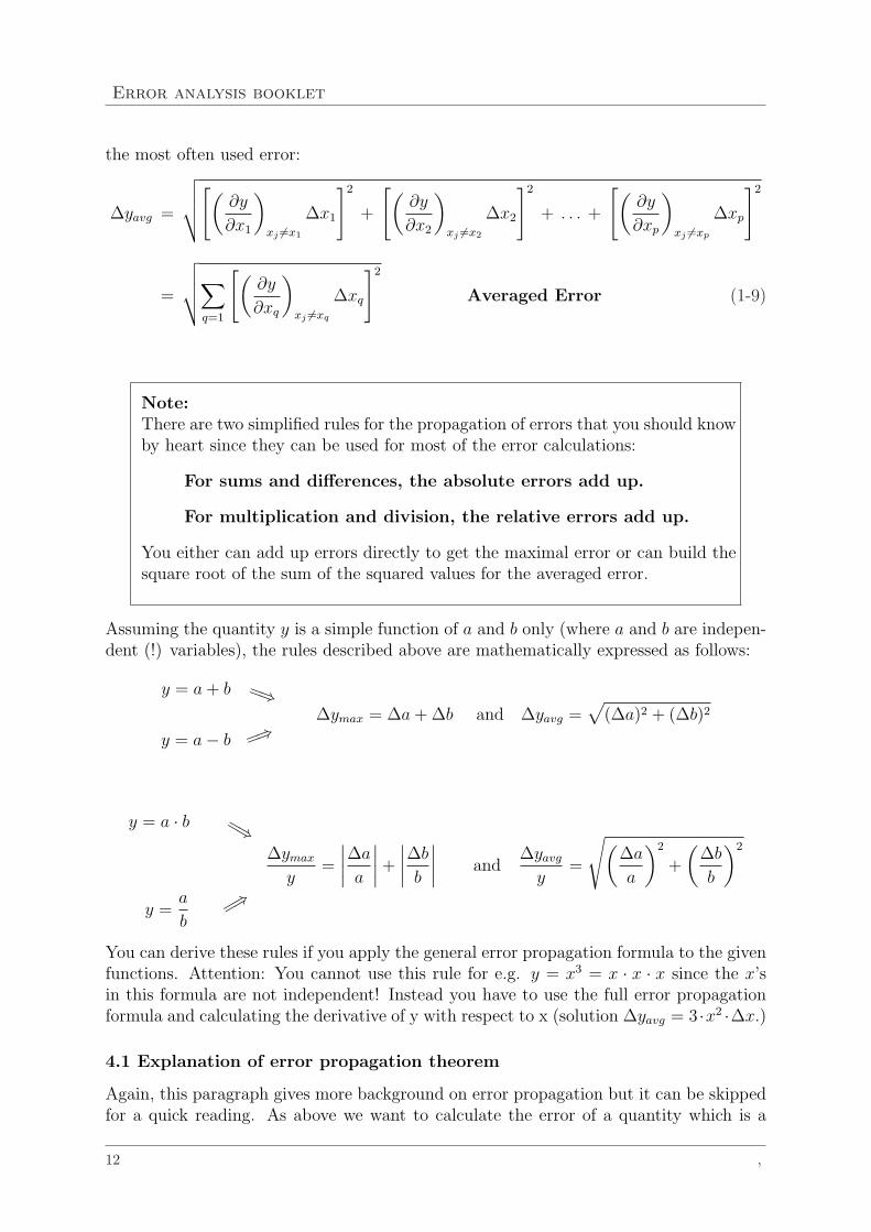
often need to be applied in order to evaluate the data and prove a functional dependencebetween the parameters expected from theoretical considerations. In order to achievethat, usually a “least squares fit” method is applied : the dataset is compared to a setof curves (e.g. polynomials) by calculating the deviations between observed data andtheoretical curves using the total sum of squared absolute differences.The minimization of the sum of the squared differences has already been applied to de-termine the mean value of a sample. For a linear function f(x) = m x + c the sum ofthe squared differences is defined as follows:

S =n∑

i=1

(yi − f(xi))2 =

n∑i=1

(yi −mxi − c)2 (1-13)

This sum will be minimized with respect to the parameters, i.e. the slope m and theconstant c, resulting in:

∂S

∂m= 0= −2

∑xi(yi −mxi − c) (1-14)

∂S

∂c= 0= −2

∑(yi −mxi − c) (1-15)

By using∑n

i=1 xi = nx and∑n

i=1 yi = ny, this set of linear equations (1-14)-(1-15) canbe solved straightforward to obtain the slope m and the intercept with the ordinate c.

m =

∑(xi − x)(yi − y)∑

(xi − x)2(1-16)

c = y −mx (1-17)

Assuming that errors in xi can be neglected and errors in yi are normal-distributed, thestandard deviation of slope σm and intercept σc can be calculated from:

σ2m = N σ2

y/D (1-18)

σ2c = σ2

y

N∑i=1

x2i /D (1-19)

with

di = yi − (mxi + c) (1-20)

σy =

√∑Ni=1 d2

i

(N − 2)(1-21)

D = N

N∑i=1

x2i −

(N∑

i=1

xi

)2

(1-22)

The regression line goes through the point (x, y) which is also called the “center of grav-ity” of the line. The quality of the fit is given by the so-called correlation coefficientR. It describes how good the data correlates to a straight line. R covers a range between



1 and 0, whereas the value 1 correspond to a perfect correlation. R is given by:

R =

∑i (xi − x) · (yi − y)√∑

i (xi − x)2 ·∑ (yi − y)2(1-23)

The uncertainty of m and c are determined by the number of measurements n and thecorrelation coefficient R2. Assuming that the yi errors are normal distributed and thatthe individual corresponding error bars have (approximately) the same size, the error ofthe slope ∆m and the error of the intercept ∆c can also be calculated by:

∣∣∣∣∆m

m

∣∣∣∣ =

√1

(n− 2)· (1−R2)

R2(1-24)

∣∣∣∣∣∆c

m√∑

i x2i

∣∣∣∣∣ =

√1

n(n− 2)· (1−R2)

R2(1-25)

5.3 Line through the origin

A special case of the linear regression is the line through the origin, where the interceptc has a value of zero. The formula of the line is reduced to y = mx. The solution andthe error of the slope could be found using the least sqare minimization

m =

∑xiyi∑x2

i

(1-26)

(∆m)2 ≈ 1

n− 1

∑(yi −mxi)

2

∑x2

i

(1-27)

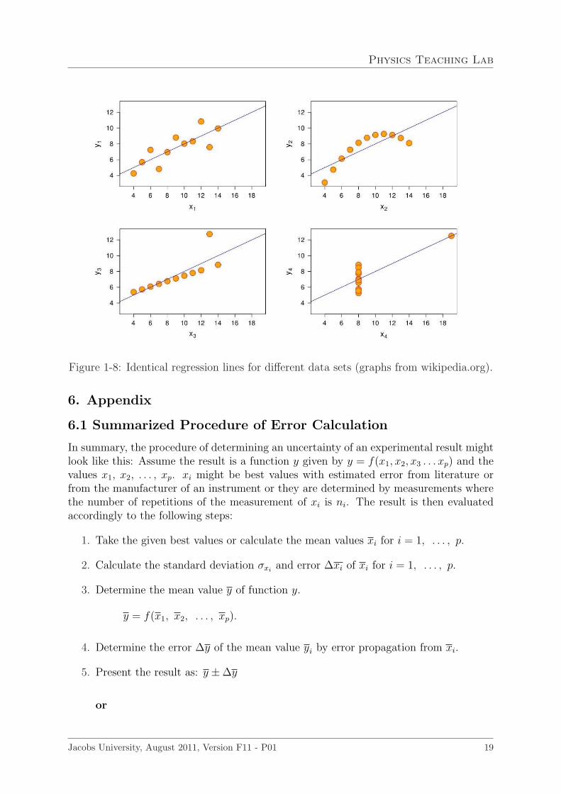
In the case of this linear fit the intercept value of zero will be weighted with infinity. Asa result the error of the slope is higher than for a line with nonzero intercept.Data analysis programs as well as most scientific calculators also offer the possibility tocalculate the linear regression line of a given data set for determination of an averagedslope and intercept. The importance of the graphical method decreases more and more.Nevertheless, especially for data sets with a low number of data points or when nonumerical programs are at hand the graphical method is still useful.Be aware that the mindless use of numerical data analysis programs has the potentialof missinterpretation of data. Before reporting the values of slope and intercept and acorrelation coefficient one has to have a look at the original graph (one indeed shouldalways plot the data not just handle numerical values!). As it can be shown, even obviousNON linear distributed data points can produce straight line fits with valid correlationcoefficients. An example is the so called Anscombe’s quartet shown in Fig. 1-8 (aftera publication from F.J. Anscombe in 1973).All data sets in this plot have the same mean value and variance in x and y and produce

identical regression lines with identical correlation coefficients. It should be clear thatplots on the right should certainly NOT be described and analysed by a straight line. Theplot at top left is OK and plot bottom left might need another check of the outliner datapoint. As a conclusion, linear regression is good for verifying a known linear dependence,but problematic for deciding if an unknown dependence is indeed linear.

18 ,


Figure 1-8: Identical regression lines for different data sets (graphs from wikipedia.org).

6. Appendix

6.1 Summarized Procedure of Error Calculation

In summary, the procedure of determining an uncertainty of an experimental result mightlook like this: Assume the result is a function y given by y = f(x1, x2, x3 . . . xp) and thevalues x1, x2, . . . , xp. xi might be best values with estimated error from literature orfrom the manufacturer of an instrument or they are determined by measurements wherethe number of repetitions of the measurement of xi is ni. The result is then evaluatedaccordingly to the following steps:

1. Take the given best values or calculate the mean values xi for i = 1, . . . , p.

2. Calculate the standard deviation σxiand error ∆xi of xi for i = 1, . . . , p.

3. Determine the mean value y of function y.

y = f(x1, x2, . . . , xp).

4. Determine the error ∆y of the mean value yi by error propagation from xi.

5. Present the result as: y ±∆y

or



for Advanced Labs present the k-corrected result for the appropriate confidencelevel in the form of:

y ± k∆y

6. Take care of significant digits when presenting the result!

6.2 Gaussian Distribution

The Gaussian or Normal Distribution describes the distribution of random statisticalvalues of a measurement around a mean value. The values accumulate around the mean,and 68% of the values are located within 1σ around the mean (see Fig.1-9).

Figure 1-9: Gaussian Distribution.

The specific function is also called a bell-shaped function and is described by:

f(x) =1√2π

· 1

σ· e− (x−µ)2

2σ2 (1-28)

with the mean value µ and the standard deviation σ. The function is symmetric aroundµ, has its maximum at µ, and tends rapidly to zero when |x− µ| becomes large comparedto σ. The points at µ ± σ are the inflection points of the curve. Another parameter tocharacterize the curve is the full width at half maximum (FWHM) or the half width atfull maximum (HWHM) which is the distance on the x-axis between the mean value andthe point where f(x) is half its maximum value. One can show that:

HWHM =√

2 ln 2 · σ = 1.17 · σ (1-29)

or very roughly HWHM ≈ σ. With that information one can easily estimate the standarddeviation of a normal distribution just by visual inspection.

20 ,

Documents

Error Analysis Booklet - Jacobs University · PDF fileError analysis booklet 1. ... K. F. Riley, M.P. Hobson, S.J. Bence: Mathematical Methods for ... cuit to deposit 0.0011180 grams