ERODE: Evaluation and Reduction ofStochastic Reaction Networks

and Differential Equationshttp://www.erode.eu/

v 1.0 — March 20, 2020

1 Introduction

ERODE is a software tool for the evaluation and reduction of stochastic reaction networks(RN) and systems of explicit first-order, autonomous ordinary differential equations (ODEs)that implements the minimization algorithms published in [1, 2, 3, 4]. ERODE has beenpresented in [5], while tutorials on it have been given in [6, 7]. At the basis of ERODE areforward and backward differential equivalence, two complementary equivalence relations overthe variables of an ODE system. Forward differential equivalence (FDE) identifies a partitionof the ODE variables for which a self-consistent aggregate ODE system can be providedwhich preserves the sums of variables within a block. Backward differential equivalence (BDE)identifies a partition whereby variables in the same block have the same solution wheneverinitialized equally. The minimization algorithms are partition-refinement algorithms thatcompute the largest equivalence that refines a given initial partition of variables.

ERODE accepts input ODE systems in two formats: a direct specification of an ODE sys-tem (close to its mathematical definition) as a collection of functions, each giving the deriva-tive for each variable; and a reaction-network (RN) specification, akin to a formal chemical

reaction network. For instance, the simple specification A + Bk−→ C describes the dy-

namics of species/variables A, B, C according to mass-action kinetics. The ODEs becomedA/dt = dB/dt = −A ·B, dC/dt = A ·B.

The choice of the input format may affect which analysis and reduction techniques areavailable. RNs induce, and can encode, ODE systems with derivatives that are multivariatepolynomials of any degree [1]. Such systems can be reduced with the specialized algorithmsof [1] (which superseded those presented in [4, 2, 5]) for computing the largest forward andbackward RN equivalences. These are equivalence relations defined syntactically on the RN

1

syntax: forward RN equivalence (FE) charactirizes FDE for this class of ODEs. Similarly,backward RN bisimulation (BE) characterizes BDE. Importantly, they enable a significantlyfaster partition-refinement algorithm than the SMT-based ones for FDE and BDE that areavailable for a generic input specification, developed in [3].

The outputs of the reduction algorithms are (hopefully) smaller ERODE specificationswhere each macro-variable represents a distinct equivalence class of species. The link be-tween a macro-variable and the members of the corresponding equivalence class is main-tained through annotations in the form of comments in the file. The format of the outputspecification (i.e., plain ODE or RN) is the same as the input.

In addition to ODEs and Reaction Networks ERODE has been recently extended to sup-port semi-explicit Differential Algebraic Equations (DAEs) in the format presented in [8].DAE systems are an extension of ODE systems where the user can express, in addition tothe differential equations, a set of algebraic constraints. Moreover, DAEs can be reduced upto BE and BDE.

2 Setting up ERODE

Installation. ERODE is a multi-platform application based on the Eclipse framework. Itdoes not require any installation process. The only requirement is a working installation ofJava 8, available at:

https://java.com/en/download/

ERODE can be downloaded from:

https://www.erode.eu/download.html

A screenshot of ERODE is shown in Fig. 1.

Updating ERODE . ERODE is actively developed, and new features will be added. Thetool can be updated to the latest version by clicking on Help→ Check for Updates.

Preparing the workspace. Upon installation the user is prompted to select the location forthe workspace. This is a directory containing all ERODE files, arranged into projects. ERODErecognizes “.ode” files. Projects and ERODE files can be created as follows:

1. Create a new ERODE project: Right click on the Project Explorer (top-left of Fig. 1),and select New→ ERODE Project. Choose a project name and click Finish.

2.A Create an ERODE file: Right click on the newly created project in the Project Explorerand choose New→ ERODE File.Hint: The combo box gives the possibility of generating a basic template file with com-ments that illustrate various parts of the language.

2.B Alternatively, it is possible to import a file from one of the supported input formats:

Matlab : a Matlab function representing the derivatives of an ODE system (extension .m);

BNG : a CRN generated with the well-established tool BioNetGen version 2.2.5-stable [9](extension .net).

2

Figure 1: A screenshot of ERODE .

LBS : a CRN written in the LBS format of the Microsoft’s tool GEC 1 (extension .lbs).

Right click on the newly created project in the Project Explorer and choose New→ Im-port BioNetGen File or New→ Import Matlab ODEs. A dialog will appear allowingfirst to choose a source folder, and to select a number files contained in there.

3 A dialog will pop-up asking to “add the Xtext nature to the project”: Click Yes.

Example project. A sample project with ERODE examples is available. To use it:

1. Download and decompress the archive available at:

https://www.erode.eu/examples.html

2. Right click on the Project Explorer, and select Import. Choose Existing Projects intoWorkspace and click Next.

3. Click on Browse... and locate the Examples folder. Tick Copy projects into workspaceand hit Finish.

Editing ERODE specifications. Upon double-clicking on an ERODE file in the Project Ex-plorer, the graphical text editor will open. The key sequence Ctrl+space (Windows/Linux)or Command+space (Mac) will enable content assist, providing contextual code suggestions.In-line markers will be used to highlight errors (and suggest fixes).

1http://research.microsoft.com/en-us/projects/gec/

3

Listing 1: Direct ODE specification.begin model ExampleODEbegin parametersr1 = 1.0 r2 = 2.0end parametersbegin initAu = 1.0 Ap = 2.0 B = 3.0AuB ApBend initbegin partition{Au,Ap}, {AuB}, {B,ApB}end partitionbegin ODE// C-style commentsd(Au) = -r1*Au + r2*Ap - 3*Au*B + 4*AuBd(Ap) = r1*Au - r2*Ap - 3*Ap*B + 4*ApBd(B) = -3*Au*B + 4*AuB - 3*Ap*B + 4*ApBd(AuB) = 3*Au*B - 4*AuBd(ApB) = 3*Ap*B - 4*ApBend ODEbegin viewsv1 = Au + Apv2 = AuBend viewsreduceBDE(reducedFile="ExampleODE_BDE.ode")end model

Listing 2: Reaction network.begin model ExampleRNbegin parametersr1 = 1.0 r2 = 2.0

end parametersbegin initAu = 1.0 Ap = 2.0 B = 3.0AuB ApB

end initbegin partition

{Au,Ap}, {AuB}end partition

begin reactionsAu -> Ap , r1Ap -> Au , r2Au + B -> AuB , 3.0AuB -> Au + B , 4.0Ap + B -> ApB , 3.0ApB -> Ap + B , 4.0

end reactionsbegin viewsv1 = Au + Apv2 = AuB

end viewssimulateODE(tEnd=1.0)end model

Running ERODE specification. To run an ERODE specification, click the ERODE icon inthe toolbar ( , top-left of Fig. 1 ). Alternatively, right-click the file in the Project Explorer, andclick Execute selected ERODE Program.

3 ERODE Language

Illustrating example. We show some of ERODE ’s features using a simple model. This isan idealized biochemical interaction between two molecules, A and B, where A can be in twostates (u for unphosphorylated and p for phosphorylated) undergoing binding/unbindingwith B. This results in five biochemical species: Au, Ap, B, AuB, and ApB. Each species isassociated with one ODE variable which models its concentration as a function of time.

Listings 1 and 2 show the two alternative specification formats for the same model (as-suming mass-action kinetics), using plain ODEs or the RN representation, respectively. List-ing 3 shows the model can be expressed in DAE format.

Specification language. The input format consists of the following parts:

i) Parameter specification;

ii) Declaration of variable names with (optional) initial conditions;

iii) Declaration of (optional) algebraic variable names with (optional) initial conditions;

iv) Initial partition of variables to be given to the reduction algorithms;

v) ODE system, either in plain format or as an RN;

4

Listing 3: DAE specification.begin model ExampleDAEbegin parametersr1 = 1.0 r2 = 2.0end parametersbegin initAu = 1.0 Ap = 2.0AuB ApBend initbegin alginitB = 3.0end alginitbegin ODEd(Au) = -r1*Au + r2*Ap - 3*Au*B + 4*AuBd(Ap) = r1*Au - r2*Ap - 3*Ap*B + 4*ApBd(AuB)= 3*Au*B - 4*AuBd(ApB)= 3*Ap*B - 4*ApBend ODEbegin algebraicB = 3 - AuB - ApBend algebraicsimulateDAE(tEnd=1)setParam(param=r2,expr=r1)reduceBDE(reducedFile="ExampleDAE_BDE.ode")end model

vi) Declaration of (optional) algebraic constraints;

vii) Observables, called views, to be tracked by the numerical solvers;

viii) Commands for ODE numerical solution, reduction, and exporting into other formats.

Alternatively, points i)-v) can be replaced by commands:

• importBNG(fileIn=<filename>) used to load “on-the-fly” a CRN generated withBioNetGen 2.2.5.

• importMRMC(fileIn=<filename>,labellingFile=<filename>) used to loada continuous time Markov chain (CTMC) in MRMC format [10], supported also byPRISM [11] and STORM [12]. A CTMC can be simply encoded as a CRN by creat-ing one species and reaction per state and transition of the CTMC, respectively. A

transition xik−→ xj is encoded as a reaction si

k−→ sj , where si and sj are the species cor-responding to states xi and xj , respectively. As shown in [3, 4] applying FDE/FE andBDE/BE corresponds to minimizing the CTMC according to the well-known notionsof ordinary and exact lumpability for CTMCs [13], respectively.

• importSBML(fileIn=<filename>) used to load “on-the-fly” a CRN modeled inthe SBML standard. This format is used, e.g., by the BioModels database [14], a well-known repository of quantitative models of biochemical systems. This functionalityhas been obtained by integrating in ERODE the SBML translator presented in [15].

• importMRMC(fileIn=<filename>,labellingFile=<filename>) used to loada continuous time Markov chain (CTMC) in MRMC format [10], supported also byPRISM [11] and STORM [12]. A CTMC can be simply encoded as a CRN by creat-ing one species and reaction per state and transition of the CTMC, respectively. A

5

transition xik−→ xj is encoded as a reaction si

k−→ sj , where si and sj are the species cor-responding to states xi and xj , respectively. As shown in [3, 4] applying FDE/FE andBDE/BE corresponds to minimizing the CTMC according to the well-known notionsof ordinary and exact lumpability for CTMCs [13], respectively.

• importAffineSystem(fileIn=<filename>,BFile=<filename>,ICFile=<filename>) used to import affine systems in format Ax = b. See [4] for more infor-mation on how to encode affine systems as CRNs. Intuitively, each entry Arow,col of A

is encoded as a reaction xcolArow,col−−−−−→ xcol + xrow to denote the monomial xcol · Arow,col

in the underlying ODE of xrow. Instead, an entry brow of b is encoded as a reaction

Ibrow−−−→ I + xrow, where I is a special species with constant value equal to 1, to denote

constant brow in the underlying ODE of xrow.

The three parameters of the command specify the files containing A, b, and the initialcondition for the variables in x, respectively. The latter might be useful to specifyinitial partitions for our reduction techniques. The file for A must have the followingcomma-separated-value format for sparse matrices:

nvar,nvar,nvarr1,c1,value1r2,c2,value2...

where nvar specifies the number of variables, while ri, ci, valuei specifies thatAri,ci = vi.

3.1 Parameter Specification

Parameters are variables that can be used to specify values of initial conditions, interactionrates, or in views. An ERODE specification might start with an optional list of numericalparameters enclosed in the parameters block. Each is specified as

parameterName = expression

where expression is an arithmetic expression involving parameter names and reals throughthe following operators: +, -, *, /, ˆ, abs, min, and max.

3.2 Variable Declaration

The mandatory init block defines all ODE variables2 of the model. Each variable is speci-fied as:

<variable> [= IC]

where IC is an arithmetic expression involving reals and parameter names as above, thatevaluates to the initial condition assigned to the variable; IC is optional with default value 0.The later use of variables not appearing in this block is considered a syntactic error. As partof its advanced quick-fix framework, ERODE collects the list of all such undefined variables,

2Throughout this document we will use the terms ‘variable’ and ‘species’ interchangeably.

6

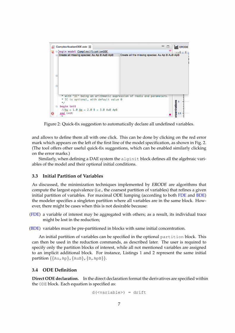
Figure 2: Quick-fix suggestion to automatically declare all undefined variables.

and allows to define them all with one click. This can be done by clicking on the red errormark which appears on the left of the first line of the model specification, as shown in Fig. 2.(The tool offers other useful quick-fix suggestions, which can be enabled similarly clickingon the error marks.)

Similarly, when defining a DAE system the alginit block defines all the algebraic vari-ables of the model and their optional initial conditions.

3.3 Initial Partition of Variables

As discussed, the minimization techniques implemented by ERODE are algorithms thatcompute the largest equivalence (i.e., the coarsest partition of variables) that refines a giveninitial partition of variables. For maximal ODE lumping (according to both FDE and BDE)the modeler specifies a singleton partition where all variables are in the same block. How-ever, there might be cases when this is not desirable because:

(FDE) a variable of interest may be aggregated with others; as a result, its individual tracemight be lost in the reduction;

(BDE) variables must be pre-partitioned in blocks with same initial concentration.

An initial partition of variables can be specified in the optional partition block. Thiscan then be used in the reduction commands, as described later. The user is required tospecify only the partition blocks of interest, while all not mentioned variables are assignedto an implicit additional block. For instance, Listings 1 and 2 represent the same initialpartition {{Au,Ap},{AuB},{B,ApB}}.

3.4 ODE Definition

Direct ODE declaration. In the direct declaration format the derivatives are specified withinthe ODE block. Each equation is specified as:

d(<variable>) = drift

7

where drift is an arithmetic expression containing ODE variables, algebraic variables (inthe case of DAE systems), parameters and reals through the operators defined in Section 3.1.This syntax identifies a class of ODEs for which the computation of differential equivalencesis decidable [3].

Reaction network format. In the RN format, ODEs are inferred from reactions in the form:

reagents -> products, rate [ identifier ]

where reagents and products are two multisets of variables. The multiplicity of a vari-able in a multiset can be defined through the + operator or with the * operator in the obviousway; that is, A + A is equivalent to 2*A. In some cases, it might be useful to assign an iden-tifier to some reactions. This can be done by adding [ identifier ] after the rate, whereidentifier identifies the reaction.

The semantics of the reaction is that it generates a negative term in the ODE correspond-ing to each reagent, and a positive term in the ODE of each product, proportionally to theirmultiplicity. Three kinds of rates are supported:

• Mass action: If rate is a variable-free expression that evaluates to a real number(as in all reactions of Listing 2), then the reaction represents a dynamics akin to thewell-known law of mass action. For example, Au + B -> AuB, 3.0 leads to a term+3 · Au · B· in the ODE of AuB, and to −3 · Au · B· it the ODEs of both Au and B.

Note. The parameter rate needs not evaluate to a positive real: this allows to encodean arbitrary ODE with polynomial derivatives into an RN [4]. When every rate doesevaluate to positive real we call the RN a chemical reaction network (CRN). It identifiesa class of models for which specific analysis options are available in ERODE . Further-more, an elementary CRN is one where the size of the reagent multiset is at most two.

• Arbitrary: ERODE also supports more generic arithmetical expressions for rates throughthe arbitrary keyword. In this case, the reaction firing rate is explicit. For instance,

Au + B -> AuB, arbitrary 3.0*Au*B

is equivalent to Au + B -> AuB, 3.0.

• Hill: ERODE also allows to specify reactions with Hill kinetics [16]. This is obtainedwith rates of form Hill K k R1 r1 R2 r2 n1 a n2 b, with k, r1 and r2 beingreal parameters, and a and b two naturals. Only binary Hill reactions (i.e., with tworeagents) are allowed. The Hill keyword is actually treated as syntactic sugar, as Hillreactions are transformed in arbitrary reactions with rate

k · Xa · Yb

(r1+ Xa) · (r2+ Yb).

3.5 DAE Definition

In the definition of Differential Algebraic Equations systems the declaration of the dynamicsof the differential variables are specified in the ODE block. The declaration of the algebraicconstraints is specified in the algebraic block. Each algebraic constraint is specified as:

8

<AlgebraicVariable> = constraint

where constraint is an arithmetic expression containing differential variables, algebraicvariables, parameters and reals through the operators defined in Section 3.1.

3.6 Views

Views represent the variables of interest to the modeller. As for ODEs, each view can bespecified as an arithmetic expression involving variables, parameters and reals. In the run-ning example the intent is to collect the total concentration of the A-molecules, regardless oftheir phosphorylation state, and the concentration of the compound AuB, respectively.

For a CRN specification, views expressions can also contain terms of form

var(s1) and covar(s1,s2)

referring, respectively, to the variance of the ODE variable s1, and to the covariance of theODE variables s1 and s2. In other words, ERODE implements the so-called linear noiseapproximation of [17], allowing to study not just the first order moments of the ODE variables,but also their variance.

3.7 ODE Solution

The numerical solution of the ODE can be obtained through the simulateODE command:

simulateODE(tEnd=<value>, steps=<value> , csvFile=<filename>,

viewPlot=<VARS&VIEWS | VARS | VIEWS | NO >,

defaultIC= <value>, computeJacobian = <true | false>,

library = <APACHE | SUNDIALS>)

It integrates the ODE system starting from the specified initial conditions up to time pointtEnd, interpolating the results at steps equally spaced time points. If the optional ar-gument csvFile is present, the plots are exported into comma-separated values formats.If the optional argument viewPlot is not present or it is set to VARS&VIEWS, then twoplots are generated, one for the the trace of each ODE variable and one for the trace of eachspecified view, respectively. The optional argument defaultIC allows to overwrite the de-fault value of unspecified initial concentrations. The optional argument library allows tochoose which solver to use. By default, the solver used is provided in the Apache library(http://commons.apache.org/proper/commons-math/). Otherwise it is possible toselect the CVODE solver provided in the library SUNDIALS [18].

In the case of elementary RN specifications, the optional argument computeJacobiancan be used to trigger the evaluation of the Jacobian matrix of the reaction network at eachsampled point. The Jacobian will be plotted and/or stored in a csv file depending on thevalue of the csvFile and viewPlot arguments.

9

3.8 DAE Solution

The numerical solution of the DAE systems can be obtained through the simulateDAEcommand:

simulateDAE(tEnd=<value>, steps=<value> , csvFile=<filename>,

viewPlot=<VARS&VIEWS | VARS | VIEWS | NO >,

defaultIC= <value>)

It solves the DAE system starting from the specified initial conditions up to time pointtEnd, interpolating the results at steps equally spaced time points. This is done usingthe IDA solver provided in the library SUNDIALS [18]. If the optional argument csvFileis present, the plots are exported into comma-separated values formats. If the optional ar-gument viewPlot is not present or it is set to VARS&VIEWS, then two plots are generated,one for the the solution of each differential or algebraic variable and one for the trace ofeach specified view, respectively. The optional argument defaultIC allows to overwritethe default value of unspecified initial concentrations.

3.9 CRN Stochastic Simulation

CRNs can also be interpreted as a stochastic system of reactions in terms of a continuous-time Markov chain (CTMC), following an established approach [19]. ERODE allows to sim-ulate sample paths, or to analyze the CRN exactly by the underlying forward equations (thechemical master equation, CME).

Stochastic simulation. Stochastic simulation is available with the command

simulateCTMC(tEnd=<value>,repeats=<value>,method=<simulationMethod>)

where tEnd represents the time horizon, repeats specifies the number of independent sim-ulations to be performed, and method allows to choose the simulation algorithm. ERODEuses the FERN library for stochastic simulation [20], which makes available the followingoptions:

• ssa: Gillepsie’s direct method;

• ssa+: Gillepsie’s direct method enhanced using dependency graphs;

• nextReaction: Next-reaction method by Gibson and Bruck;

• tauLeapingAbs, tauLeapingRelProp and tauLeapingRelPop: three variants ofthe Tau-leaping algorithm, providing different error bounds;

• maximalTimeStep: Maximal time step method by Puchalka.

Details on all the supported simulation methods can be found in [20].When more than one sample is requested, ERODE computes the average trajectories

from time 0 to tEnd. The user can specify further options using the arguments steps,viewPlot, csvFile and defaultIC, similarly to the ODE numerical solution.

10

For a more efficient implementation of these and more simulation algorithms we suggestthe user to export the model in StochKit format as described below and to use the StochKittool [22] 3 as simulation engine.

Chemical Master Equation. ERODE can explicitly build the CTMC underlying a chemicalreaction network through its CME. This is stored in an ERODE file as a CRN having onereaction (with unary reagents and unary products) per transition, using the command:

generateCME(fileOut=<filename>)

If the output ERODE file is analyzed with simulateODE, this corresponds to numericallyintegrating the forward equations of the CTMC. As shown in [3, 4] applying FDE/FE andBDE/BE corresponds to minimizing the CTMC according to the well-known notions of or-dinary and exact lumpability for CTMCs [13], respectively.

3.10 Reduction Commands

All ODE reduction commands share the common signature

reduce<kind>(prePartition=<NO | IC | USER>, reducedFile=<name>)

where kind can be FDE, BDE, FE, or BE. The ODE input format affects which reduction op-tions are available. For an ODE system defined directly, only FDE and BDE are enabled. FEand BE are additionally available for reaction networks yielding polynomial ODE systemsof any degree [1]. For a DAE system only BE and BDE are enabled. This is imposed byrestricting to mass-action type rate expressions.

In addition, ERODE supports a further reduction technique for the stochastic semanticsof (chemical) reaction networks [19]:

• reduceSMB: an RN equivalence in the style of FE which induces ordinary lumpabilityon the CME underlying an elementary mass-action CRN [21].

• reduceSE: an generalization of reduceSMB to mass-action CRNs pf any arity. Thepaper presenting it is currently under review.

The option prePartition defines the initial partition passed to the minimization al-gorithm. The maximal aggregation is obtained with the NO option. If it is set to IC, theinitial partition to be refined is built according to the constraints given by the initial condi-tions: variables are in the same initial block whenever their initial conditions (specified inthe init block) are equal. If the option is set to USER, then the partition specified in thepartition block will be used. In the case of BDE/BE the reduction may not be consistentwith the initial condition, in the sense that the user can specify a block with two variablesthat have different initial conditions, breaking the side condition imposed by these equiva-lences: ERODE will issue a warning to the user in this case.

The argument reducedFile generates a reduced model in the same format as the in-put, following the model-to-model transformation algorithms presented in [1] (for FE andBE) and [3] (for FDE and BDE). In all cases, in the reduced ERODE model there will be one

3Available at https://github.com/StochSS/StochKit

11

variable for each computed equivalence class. The name of the variable is (arbitrarily) givenby the first variable name in that block, according to a lexicographical order. All membersof each equivalence class are reported as annotations in comments. For the BDE case, eachreduced variable represents any single variable of the corresponding equivalence class. In-stead, in the other cases (FE, BE, and FDE) each variable represents the sum of all variablesin the corresponding equivalence class.

Any reduction command can be preceded by the keyword ’this =’ which has the effectof updating the currently loaded model with its reduction. This is particularly useful in casefurther commands have to be executed on the result of an execution (e.g., further reductions,analysis, etc).

3.11 Exporting Options

Conversion options. An explicit ODE specification can be converted in the RN format (andvice versa) using

write(fileOut=fileName,format=<ODE | NET |MA-RN>)

If the format option is set to ODE, then the target file will be in explicit ODE format, whilewith the RN option an RN will be generated. If the specification to be exported is an explicitODE with derivatives given by multivariate polynomials of degree at most two, the MA-RNwill use the encoding of [4] to output a mass-action RN.

Export to third-party languages. The command:

export<format>(fileIn=fileName)

exports ERODE files into several different target third-party languages:

Matlab : a Matlab function representing the derivatives of an ODE system (extension .m);

BNG : a CRN generated with the well-established tool BioNetGen version 2.2.5-stable [9](extension .net). Available for CRN specifications only;

SBML : the well-known SBML interchange format (http://sbml.org) (extension .sbml).

LBS : Exporting support is offered for the LBS format of the Microsoft’s tool GEC 4 (exten-sion .lbs). Available for CRN specifications only. ERODE ’s analysis options are nottranslated into LBS directives.

Modelica : a Modelica model representing the ODE/DAE system compatible with Open-Modelica (extension .mo). The optional parameter exportICOfAlgebraic allowsthe user to explicitly export the initial conditions of the algebraic variables. By defaultthis parameter is set to false as OpenModelica can infer the initial condition of thealgebraic variables automatically.

StochKit : a CRN in the format of to StochKit tool [22] (extension .xml). StochKit is asimulation engine offering efficient implementations of the most popular algorithmsfor the stochastic simulation of CRN.

4http://research.microsoft.com/en-us/projects/gec/

12

Listing 4: FDE reduction.begin model ExampleODE_FDEbegin parametersr1 = 1.0r2 = 2.0end parametersbegin initAu = 1.0 + 2.0B = 3.0AuBend initbegin ODEd(Au) = - 3*Au*B + 4*AuBd(B) = - 3*Au*B + 4*AuBd(AuB) = 3*Au*B - 4*AuBend ODE//Comments associated to the species//Au: Block {Au, Ap}//B: Block {B}//AuB: Block {AuB, ApB}end model

Listing 5: BDE reduction.begin model ExampleODE_BDEbegin parametersr1 = 1.0r2 = 1.0end parametersbegin initAu = 1.0B = 3.0AuBend initbegin ODEd(Au) = - 3*Au*B + 4*AuBd(B) = - 6*Au*B + 8*AuBd(AuB) = 3*Au*B - 4*AuBend ODE//Comments associated to the species//Au: Block {Au, Ap}//B: Block {B}//AuB: Block {AuB, ApB}end model

3.12 Further Commands

It is possible to change the value of a parameter or the initial concentration of a variable:

setIC(species=x0,expr=1) setParam(param=p1,expr=2)

These are useful in case one is interested in considering different variants of a given ERODEspecification.

4 Examples

In this section we show a number of scenarios using variants of the running example.

Direct specification/FDE. The running example can be reduced according to FDE. Indeed,it is not difficult to see that one can write an ODE system for B and the sum of variablesAu+Ap and AuB+ApB, corresponding to the FDE partition {{Au,Ap},{B},{AuB,ApB}}.

However, this reduction is not found by ERODE if the pre-partitioning flag is set to USER.In fact, the above FDE partition is not a refinement of the user specified one, where AuB is ina singleton block. The output file for the case without pre-partitioning is shown in Listing 4,which also shows how the association between the original ODE variables and those in thereduced model is maintained by automatically annotating the output file with commentsalongside the new variables.5

Direct specification/BDE. The partition {{Au,Ap},{B},{AuB,ApB}} can also be shown tobe a BDE if r1 is equal to r2. Intuitively, this would capture the fact that the phosphorylationstate of A does not impact the way in which the molecules react within this model. Thus, itwould be enough to consider either state as a representative of the dynamics. However, if

5Output files have been typographically adjusted to improve presentation.

13

Listing 6: BE reduction of RN in Listing 2.begin model ExampleRN_BEbegin parametersr1 = 1.0 r2 = 1.0end parametersbegin initAu = 1.0+2.0 B = 3.0 AuBend initbegin reactionsAu + B -> AuB , 3.0AuB -> Au + B , 4.0end reactions//Comments associated to the species//Au: Block {Au, Ap}//B: Block {B}//AuB: Block {AuB, ApB}end model

Listing 7: BDE reduction of DAE in Listing 3.begin model ExampleDAE_BDEbegin parametersr1 = 1.0r2 = 1.0end parametersbegin initAu = 1.0AuBend initbegin alginitB = 3.0end alginitbegin ODEd(Au) = (-r1)*Au+(r2*Au-3*Au*B)+4*AuBd(AuB) = 3*Au*B-4*AuBend ODEbegin algebraicB = 3-AuB-AuBend algebraic//Comments associated to the species//B: Block {B}//Au: Block {Au,Ap}//AuB: Block {AuB,ApB}end model

BDE is run with pre-partitioning set ot IC, this partition violates the initial conditions forAu and Ap; indeed, no reduction is found in this case. Instead, if the pre-partitioning isdisabled, then the above partition is the coarsest refinement; the user is warned about theinconsistency with the initial conditions. The BDE reduction algorithm rewrites the ODEsof the representatives of each equivalence class. The initial condition for the ODE of therepresentative is equal to that of the corresponding variable in the original model. The BDEreduction without pre-partitioning for r1=1.0 and r2=1.0 is given in Listing 5.

Differential Algebraic Equations/BDE. Similarly to the ODE with the direct specification,the partition {{Au,Ap},{B},{AuB,ApB}} can also be shown to be a BDE for the DAE sys-tem in Listing 3 if r1 is equal to r2. In this case, the BDE reduction algorithm rewrites theDAEs of the representatives of each equivalence class. The initial condition for the DAE ofthe representative is equal to that of the corresponding variable in the original model. TheBDE reduction without pre-partitioning for r1=1.0 and r2=1.0 is given in Listing 7.

RN/Equivalences. When the input is an elementary RN, the reduction algorithm for FEand BE of [1] can be used. It is based on Paige and Tarjan’s coarsest-refinement algorithm [23]and quantitative extensions thereof [24]. The FE and BE equivalences of the model of List-ing 2 are the same as those computed using FDE and BDE. For example, the result of BEreduction is provided in Listing 6. As for BDE, we considered the case r1 = 1.0 and r2 = 1.0without pre-partitioning. The comments at the end of the model confirm that we computedthe same equivalence as in Listing 5. However, it can be shown that the underlying ODEsof the reduced model do not correspond to those of Listing 5. This is expected, because asdiscussed in Section 3.10, in a BDE reduced model each variable describes any single vari-able of the corresponding equivalence class. Instead, in a BE reduced model each variabledescribes the sum of all variables in the corresponding equivalence class.

14

Listing 8: Curried ODE.begin model ExampleODECurriedbegin initAu = 1.0 Ap = 2.0 B = 3.0AuB ApBr1 = 1.0 r2 = 2.0end initbegin partition{Au,Ap}, {AuB}, {B,ApB}, {r1,r2}end partitionbegin ODEd(Au) = -r1*Au + r2*Ap - 3*Au*B + 4*AuBd(Ap) = r1*Au - r2*Ap - 3*Ap*B + 4*ApBd(B) = -3*Au*B + 4*AuB - 3*Ap*B + 4*ApBd(AuB) = 3*Au*B - 4*AuBd(ApB) = 3*Ap*B - 4*ApBd(r1) = 0d(r2) = 0end ODEbegin viewsv1 = Au + Apv2 = AuBend viewsend model

Listing 9: Curried RN.begin model ExampleRNCurriedbegin initAu = 1.0 Ap = 2.0 B = 3.0AuB ApBr1 = 1.0 r2 = 2.0

end initbegin partition

{Au,Ap}, {AuB}, {r1,r2}end partition

begin reactionsAu + r1-> Ap + r1 , 1Ap + r2-> Au + r2 , 1Au + B -> AuB , 3.0AuB -> Au + B , 4.0Ap + B -> ApB , 3.0ApB -> Ap + B , 4.0

end reactionsbegin viewsv1 = Au + Apv2 = AuB

end viewssimulateODE(tEnd=1.0)end model

Parameter-independent reductions. The reductions implemented in ERODE depend onthe values of the parameters present in the model. Without adding new theory, it is pos-sible to consider parameter-independent variants of such reductions. The idea consists inperforming a sort of currying of the paremeters in the model transforming them in variables.Such new variable are initialized with the value of the parameter, and have 0-derivative.Listings 8 and 9 contain the models from Listings 1 and 2, respectively, after applying thistransformation to the parameters r1 and r2. Notably, the dynamics of the model are notaffected by this transformation. On the other hand, given that our reduction techniques donot use the initial values of the variables, we have that the obtained reductions hold for anyvalue of the parameters r1, and r2. Such models can be obtained by the original ones usingthe following command:

this = curry(paramsToCurry=<ALL | [param1, param2, ...]>)

The execution of this command has the effect of replacing the currently loaded modelwith its curried version, therefore any other command can be used to reduce it or to exportit in a file.

References

[1] Luca Cardelli, Mirco Tribastone, Max Tschaikowski, and Andrea Vandin. Maximal ag-gregation of polynomial dynamical systems. National Academy of Sciences. Proceedings,2017.

[2] Luca Cardelli, Mirco Tribastone, Max Tschaikowski, and Andrea Vandin. Forward andbackward bisimulations for chemical reaction networks. In CONCUR, 2015.

[3] Luca Cardelli, Mirco Tribastone, Max Tschaikowski, and Andrea Vandin. Symboliccomputation of differential equivalences. In POPL, 2016.

15

[4] Luca Cardelli, Mirco Tribastone, Max Tschaikowski, and Andrea Vandin. Efficientsyntax-driven lumping of differential equations. In TACAS, 2016.

[5] Luca Cardelli, Mirco Tribastone, Andrea Vandin, and Max Tschaikowski. ERODE: Atool for the evaluation and reduction of ordinary differential equations. In Tools andAlgorithms for the Construction and Analysis of Systems — 23rd International Conference,TACAS, 2017.

[6] Andrea Vandin and Mirco Tribastone. Quantitative abstractions for collective adaptivesystems. In Formal Methods for the Quantitative Evaluation of Collective Adaptive Systems- 16th International School on Formal Methods for the Design of Computer, Communication,and Software Systems, SFM, pages 202–232, 2016.

[7] Mirco Tribastone and Andrea Vandin. Speeding up stochastic and deterministic simula-tion by aggregation: an advanced tutorial. In 2018 Winter Simulation Conference (WSC),2018.

[8] G. Yu. Kulikov. Numerical methods solving the semi-explicit differential-algebraicequations by implicit multistep fixed stepsize methods. Korean Journal of Computational& Applied Mathematics, 4(2):281–318, 1997.

[9] Michael L. Blinov, James R. Faeder, Byron Goldstein, and William S. Hlavacek. Bionet-gen: software for rule-based modeling of signal transduction based on the interactionsof molecular domains. Bioinformatics, 20(17):3289–3291, 2004.

[10] J.-P. Katoen, M. Khattri, and I.S. Zapreev. A Markov Reward Model Checker. In QEST,pages 243–244, 2005.

[11] M. Kwiatkowska, G. Norman, and D. Parker. PRISM 4.0: Verification of probabilisticreal-time systems. In G. Gopalakrishnan and S. Qadeer, editors, Proc. 23rd InternationalConference on Computer Aided Verification (CAV’11), volume 6806 of LNCS, pages 585–591. Springer, 2011.

[12] Christian Dehnert, Sebastian Junges, Joost-Pieter Katoen, and Matthias Volk. A stormis coming: A modern probabilistic model checker. In Rupak Majumdar and ViktorKuncak, editors, Computer Aided Verification, pages 592–600, Cham, 2017. Springer In-ternational Publishing.

[13] Peter Buchholz. Exact and Ordinary Lumpability in Finite Markov Chains. Journal ofApplied Probability, 31(1):59–75, 1994.

[14] Chen Li, Marco Donizelli, Nicolas Rodriguez, Harish Dharuri, Lukas Endler, Vijay-alakshmi Chelliah, Lu Li, Enuo He, Arnaud Henry, Melanie I. Stefan, Jacky L. Snoep,Michael Hucka, Nicolas Le Novere, and Camille Laibe. BioModels Database: Anenhanced, curated and annotated resource for published quantitative kinetic models.BMC Systems Biology, 4:92, Jun 2010.

[15] Isabel Cristina Perez-Verona, Mirco Tribastone, and Andrea Vandin. A large-scale as-sessment of exact model reduction in the biomodels repository. In Computational Meth-ods in Systems Biology - 17th International Conference, CMSB 2019, Trieste, Italy, September18-20, 2019, Proceedings, pages 248–265, 2019.

16

[16] Eberhard O. Voit. Biochemical systems theory: A review. ISRN Biomathematics, 2013:53,2013.

[17] Luca Bortolussi and Roberta Lanciani. Quantitative Evaluation of Systems: 10th Interna-tional Conference, QEST 2013, Buenos Aires, Argentina, August 27-30, 2013. Proceedings,chapter Model Checking Markov Population Models by Central Limit Approximation,pages 123–138. Springer Berlin Heidelberg, Berlin, Heidelberg, 2013.

[18] Alan C Hindmarsh, Peter N Brown, Keith E Grant, Steven L Lee, Radu Serban, Dan EShumaker, and Carol S Woodward. SUNDIALS: Suite of nonlinear and differential/al-gebraic equation solvers. ACM Transactions on Mathematical Software (TOMS), 31(3):363–396, 2005.

[19] D.T. Gillespie. Exact stochastic simulation of coupled chemical reactions. Journal ofPhysical Chemistry, 81(25):2340–2361, December 1977.

[20] Florian Erhard, Caroline C. Friedel, and Ralf Zimmer. FERN - a Java framework forstochastic simulation and evaluation of reaction networks. BMC Bioinformatics, 9(1):356,2008.

[21] Luca Cardelli, Mirco Tribastone, Max Tschaikowski, and Andrea Vandin. Syntacticmarkovian bisimulation for chemical reaction networks. In Models, Algorithms, Logicsand Tools - Essays Dedicated to Kim Guldstrand Larsen on the Occasion of His 60th Birthday,pages 466–483, 2017.

[22] Kevin R. Sanft, Sheng Wu, Min K. Roh, Jin Fu, Rone Kwei Lim, and Linda R. Pet-zold. Stochkit2: software for discrete stochastic simulation of biochemical systems withevents. Bioinform., 27(17):2457–2458, 2011.

[23] R. Paige and R. Tarjan. Three partition refinement algorithms. SIAM Journal on Comput-ing, 16(6):973–989, 1987.

[24] Antti Valmari and Giuliana Franceschinis. Simple o(m log n) time Markov chain lump-ing. In TACAS, 2010.

17