Embed Size (px)
Citation preview
Veriûed error bounds for multiple roots ofsystems of nonlinear equations
Stef GraillatLIP6/PEQUAN, Sorbonne Universités, UPMC Univ Paris 06, CNRS
Joint work with SiegfriedM. Rump
Journées méthodes de subdivisions pour les systèmes singuliersIRCCyN, Nantes, December 15-16, 2014
S. Graillat (Univ. Paris 6) Verified error bounds for multiple roots 1 / 42
General motivations: self-validating methods
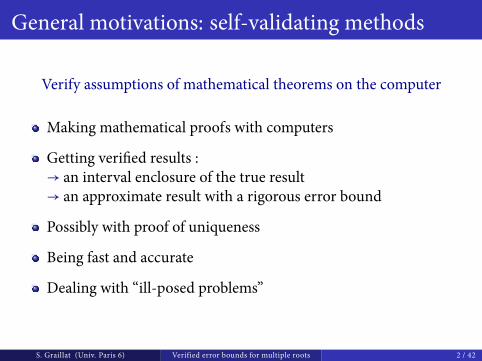
Verify assumptions ofmathematical theorems on the computer
Making mathematical proofs with computers
Getting veriûed results :→ an interval enclosure of the true result→ an approximate result with a rigorous error bound
Possibly with proof of uniqueness
Being fast and accurate
Dealing with “ill-posed problems”
S. Graillat (Univ. Paris 6) Verified error bounds for multiple roots 2 / 42
General motivations (cont’d)
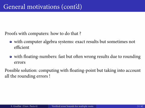
Proofs with computers: how to do that ?
with computer algebra systems: exact results but sometimes noteõcient
with �oating-numbers: fast but o�en wrong results due to roundingerrors
Possible solution: computing with �oating-point but taking into accountall the rounding errors !
S. Graillat (Univ. Paris 6) Verified error bounds for multiple roots 3 / 42
Outline of the talk
1 Principle of self-validating methods
2 Multiple roots of polynomial systems
3 Numerical experiments
S. Graillat (Univ. Paris 6) Verified error bounds for multiple roots 4 / 42

Outline of the talk
1 Principle of self-validating methods
2 Multiple roots of polynomial systems
3 Numerical experiments
S. Graillat (Univ. Paris 6) Verified error bounds for multiple roots 5 / 42
Proving that amatrix is nonsingular
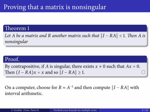
heorem 1Let A be amatrix and R another matrix such that ∥I − RA∥ < 1. hen A isnonsingular
Proof.By contrapositive, if A is singular, there exists x ≠ 0 such that Ax = 0.hen (I − RA)x = x and so ∥I − RA∥ ≥ 1.
On a computer, choose for R ≈ A−1 and then compute ∥I − RA∥ withinterval arithmetic.
S. Graillat (Univ. Paris 6) Verified error bounds for multiple roots 6 / 42
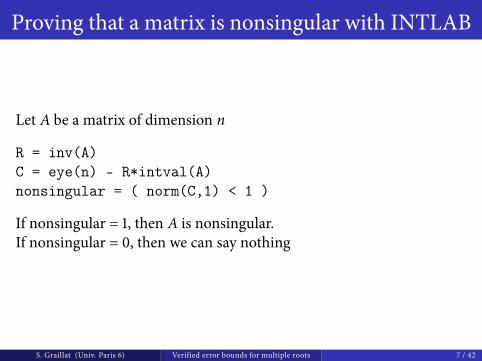
Proving that amatrix is nonsingular with INTLAB
Let A be amatrix of dimension n
R = inv(A)C = eye(n) - R*intval(A)nonsingular = ( norm(C,1) < 1 )
If nonsingular = 1, then A is nonsingular.If nonsingular = 0, then we can say nothing
S. Graillat (Univ. Paris 6) Verified error bounds for multiple roots 7 / 42
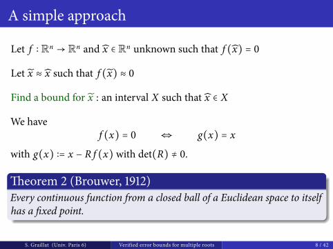
A simple approach
Let f ∶ Rn → Rn and x ∈ Rn unknown such that f (x) = 0
Let x ≈ x such that f (x) ≈ 0
Find a bound for x : an interval X such that x ∈ X
We havef (x) = 0 ⇔ g(x) = x
with g(x) ∶= x − R f (x) with det(R) ≠ 0.
heorem 2 (Brouwer, 1912)Every continuous function from a closed ball of a Euclidean space to itselfhas a ûxed point.
S. Graillat (Univ. Paris 6) Verified error bounds for multiple roots 8 / 42
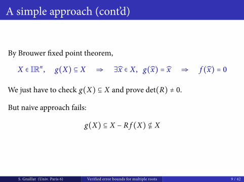
A simple approach (cont’d)
By Brouwer ûxed point theorem,
X ∈ IRn , g(X) ⊆ X ⇒ ∃x ∈ X , g(x) = x ⇒ f (x) = 0
We just have to check g(X) ⊆ X and prove det(R) ≠ 0.
But naive approach fails:
g(X) ⊆ X − R f (X) ⊈ X
S. Graillat (Univ. Paris 6) Verified error bounds for multiple roots 9 / 42
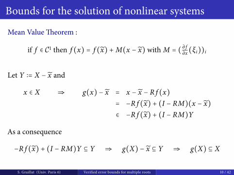
Bounds for the solution of nonlinear systems
Mean Valueheorem :
if f ∈ C1 then f (x) = f (x) +M(x − x) with M = ( ∂ f∂x (ξi))i
Let Y ∶= X − x and
x ∈ X ⇒ g(x) − x = x − x − R f (x)= −R f (x) + (I − RM)(x − x)∈ −R f (x) + (I − RM)Y
As a consequence
−R f (x) + (I − RM)Y ⊆ Y ⇒ g(X) − x ⊆ Y ⇒ g(X) ⊆ X
S. Graillat (Univ. Paris 6) Verified error bounds for multiple roots 10 / 42
Bounds for the solution of nonlinear systems(cont’d)
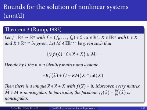
heorem 3 (Rump, 1983)Let f ∶ Rn → Rn with f = ( f1, . . . , fn) ∈ C1, x ∈ Rn, X ∈ IRn with 0 ∈ Xand R ∈ Rn×n be given. Let M ∈ IRn×n be given such that
{∇ fi(ζ) ∶ ζ ∈ x + X} ⊆ Mi ,∶ .
Denote by I the n × n identity matrix and assume
−R f (x) + (I − RM)X ⊆ int(X).
hen there is a unique x ∈ x + X with f (x) = 0. Moreover, every matrixM ∈ M is nonsingular. In particular, the Jacobian J f (x) = ∂ f
∂x (x) isnonsingular.
S. Graillat (Univ. Paris 6) Verified error bounds for multiple roots 11 / 42
Remark
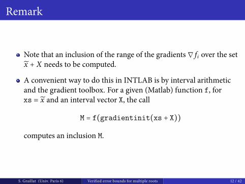
Note that an inclusion of the range of the gradients ∇ fi over the setx + X needs to be computed.
A convenient way to do this in INTLAB is by interval arithmeticand the gradient toolbox. For a given (Matlab) function f, forxs = x and an interval vector X, the call
M = f(gradientinit(xs + X))
computes an inclusion M.
S. Graillat (Univ. Paris 6) Verified error bounds for multiple roots 12 / 42

Outline of the talk
1 Principle of self-validating methods
2 Multiple roots of polynomial systems
3 Numerical experiments
S. Graillat (Univ. Paris 6) Verified error bounds for multiple roots 13 / 42
Veriûcation ofmultiple roots
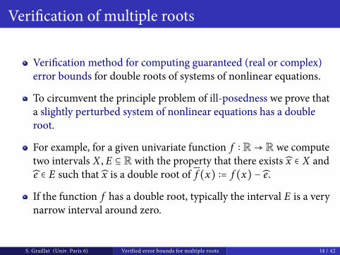
Veriûcation method for computing guaranteed (real or complex)error bounds for double roots of systems of nonlinear equations.
To circumvent the principle problem of ill-posedness we prove thata slightly perturbed system of nonlinear equations has a doubleroot.
For example, for a given univariate function f ∶ R→ R we computetwo intervals X , E ⊆ R with the property that there exists x ∈ X ande ∈ E such that x is a double root of f (x) ∶= f (x) − e.
If the function f has a double root, typically the interval E is a verynarrow interval around zero.
S. Graillat (Univ. Paris 6) Verified error bounds for multiple roots 14 / 42
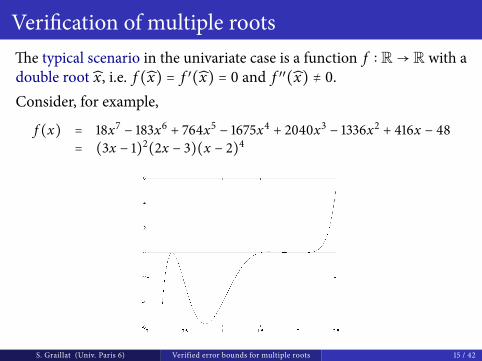
Veriûcation ofmultiple rootshe typical scenario in the univariate case is a function f ∶ R→ R with adouble root x, i.e. f (x) = f ′(x) = 0 and f ′′(x) ≠ 0.Consider, for example,
f (x) = 18x7− 183x6
+ 764x5 − 1675x4+ 2040x3
− 1336x2+ 416x − 48
= (3x − 1)2(2x − 3)(x − 2)4
S. Graillat (Univ. Paris 6) Verified error bounds for multiple roots 15 / 42
Veriûcation ofmultiple roots
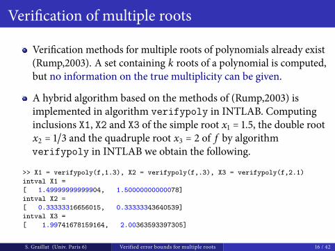
Veriûcation methods for multiple roots of polynomials already exist(Rump,2003). A set containing k roots of a polynomial is computed,but no information on the truemultiplicity can be given.
A hybrid algorithm based on themethods of (Rump,2003) isimplemented in algorithm verifypoly in INTLAB. Computinginclusions X1, X2 and X3 of the simple root x1 = 1.5, the double rootx2 = 1/3 and the quadruple root x3 = 2 of f by algorithmverifypoly in INTLAB we obtain the following.
>> X1 = verifypoly(f,1.3), X2 = verifypoly(f,.3), X3 = verifypoly(f,2.1)intval X1 =[ 1.49999999999904, 1.50000000000078]intval X2 =[ 0.33333316656015, 0.33333343640539]intval X3 =[ 1.99741678159164, 2.00363593397305]
S. Graillat (Univ. Paris 6) Verified error bounds for multiple roots 16 / 42
Veriûcation ofmultiple roots (cont’d)
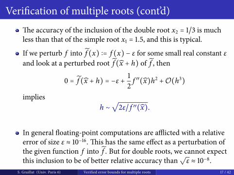
he accuracy of the inclusion of the double root x2 = 1/3 is muchless than that of the simple root x1 = 1.5, and this is typical.
If we perturb f into f (x) ∶= f (x) − ε for some small real constant εand look at a perturbed root f (x + h) of f , then
0 = f (x + h) = −ε + 12f ′′(x)h2 +O(h3)
impliesh ∼
√2ε/ f ′′(x).
In general �oating-point computations are aøicted with a relativeerror of size ε ≈ 10−16. his has the same eòect as a perturbation ofthe given function f into f . But for double roots, we cannot expectthis inclusion to be of better relative accuracy than
√ε ≈ 10−8.
S. Graillat (Univ. Paris 6) Verified error bounds for multiple roots 17 / 42
Dealing with double roots
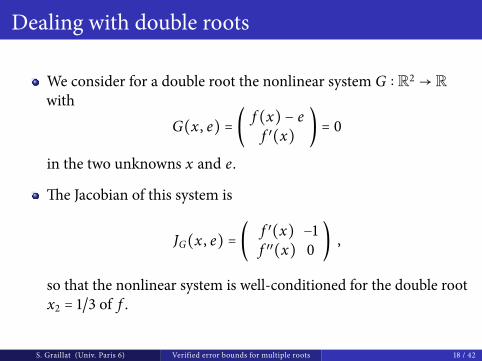
We consider for a double root the nonlinear system G ∶ R2 → Rwith
G(x , e) = ( f (x) − ef ′(x) ) = 0
in the two unknowns x and e.
he Jacobian of this system is
JG(x , e) = ( f ′(x) −1f ′′(x) 0 ) ,
so that the nonlinear system is well-conditioned for the double rootx2 = 1/3 of f .
S. Graillat (Univ. Paris 6) Verified error bounds for multiple roots 18 / 42
Dealing with double roots (cont’d)
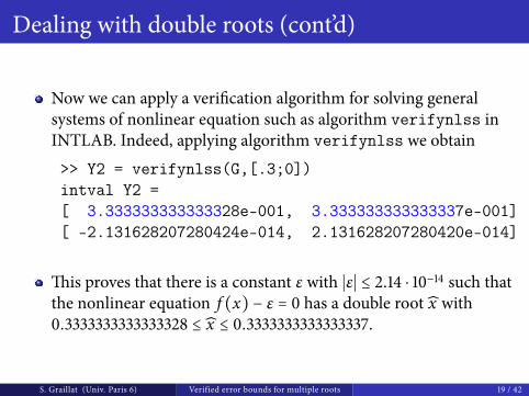
Now we can apply a veriûcation algorithm for solving generalsystems of nonlinear equation such as algorithm verifynlss inINTLAB. Indeed, applying algorithm verifynlss we obtain
>> Y2 = verifynlss(G,[.3;0])intval Y2 =[ 3.333333333333328e-001, 3.333333333333337e-001][ -2.131628207280424e-014, 2.131628207280420e-014]
his proves that there is a constant ε with ∣ε∣ ≤ 2.14 ⋅ 10−14 such thatthe nonlinear equation f (x) − ε = 0 has a double root x with0.3333333333333328 ≤ x ≤ 0.3333333333333337.
S. Graillat (Univ. Paris 6) Verified error bounds for multiple roots 19 / 42

Dealing with double roots (cont’d)
We presented the previous approach in preparation for themultivariate case;
However, for univariate nonlinear functions wemay proceedmoredirectly.
Suppose X ∈ IR is an inclusion of a root x of f ′, and use theinterval evaluation of f at X to compute E ∈ IR with f (X) ⊆ E. Inparticular f (x) ∈ E, so that there exists e ∈ E such that the functiong(x) ∶= f (x) − e satisûes g(x) = g′(x) = 0.
If,moreover, the inclusion X is computed by a veriûcation method,then x is a unique root of f ′ in X, and x is proved to be a doubleroot of g.
S. Graillat (Univ. Paris 6) Verified error bounds for multiple roots 20 / 42
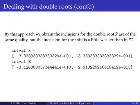
Dealing with double roots (cont’d)
By this approach we obtain the inclusions for the double root x are of thesame quality, but the inclusion for the shi� is a little weaker than in Y2:
intval X =[ 3.333333333333329e-001, 3.333333333333339e-001]intval E =[ -3.126388037344441e-013, 2.913225216616412e-013]
S. Graillat (Univ. Paris 6) Verified error bounds for multiple roots 21 / 42
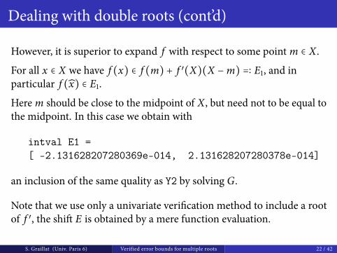
Dealing with double roots (cont’d)
However, it is superior to expand f with respect to some point m ∈ X.
For all x ∈ X we have f (x) ∈ f (m) + f ′(X)(X −m) =∶ E1, and inparticular f (x) ∈ E1.
Here m should be close to themidpoint of X, but need not to be equal tothemidpoint. In this case we obtain with
intval E1 =[ -2.131628207280369e-014, 2.131628207280378e-014]
an inclusion of the same quality as Y2 by solving G.
Note that we use only a univariate veriûcation method to include a rootof f ′, the shi� E is obtained by amere function evaluation.
S. Graillat (Univ. Paris 6) Verified error bounds for multiple roots 22 / 42
hemultivariate case
Let a suitably smooth function f ∶ Rn → Rn and x ∈ Rn be givensuch that f (x) = 0 and the Jacobian of f at x is singular.
A standard veriûcation method such as verifynlssmust failbecause with an inclusion of a root the nonsingularity of theJacobian at the root is proved as well.
Again it is an ill-posed problem and we need some regularizationtechnique.
S. Graillat (Univ. Paris 6) Verified error bounds for multiple roots 23 / 42
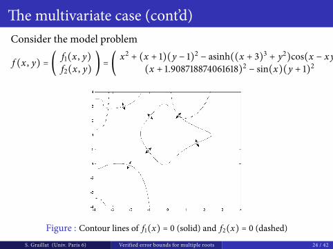
hemultivariate case (cont’d)Consider themodel problem
f (x , y) = (f1(x , y)f2(x , y)
) = (x2+ (x + 1)(y − 1)2
− asinh((x + 3)3+ y2
)cos(x − xy)(x + 1.908718874061618)2
− sin(x)(y + 1)2 ) = 0
Figure : Contour lines of f1(x) = 0 (solid) and f2(x) = 0 (dashed)
S. Graillat (Univ. Paris 6) Verified error bounds for multiple roots 24 / 42
hemultivariate case (cont’d)
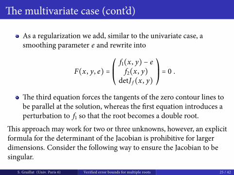
As a regularization we add, similar to the univariate case, asmoothing parameter e and rewrite into
F(x , y, e) =⎛⎜⎝
f1(x , y) − ef2(x , y)
detJ f (x , y)
⎞⎟⎠= 0 .
he third equation forces the tangents of the zero contour lines tobe parallel at the solution, whereas the ûrst equation introduces aperturbation to f1 so that the root becomes a double root.
his approach may work for two or three unknowns, however, an explicitformula for the determinant of the Jacobian is prohibitive for largerdimensions. Consider the following way to ensure the Jacobian to besingular.
S. Graillat (Univ. Paris 6) Verified error bounds for multiple roots 25 / 42
hemultivariate case (cont’d)
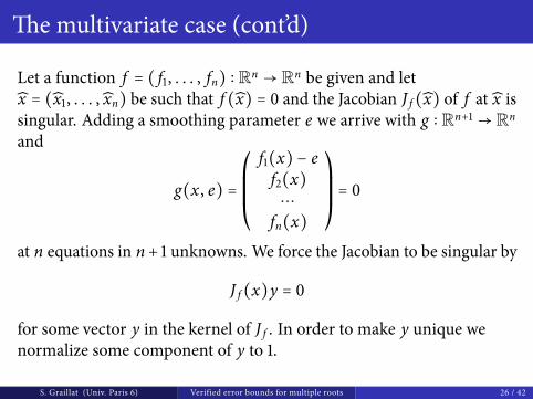
Let a function f = ( f1, . . . , fn) ∶ Rn → Rn be given and letx = (x1, . . . , xn) be such that f (x) = 0 and the Jacobian J f (x) of f at x issingular. Adding a smoothing parameter e we arrive with g ∶ Rn+1 → Rn
and
g(x , e) =⎛⎜⎜⎜⎝
f1(x) − ef2(x)⋯fn(x)
⎞⎟⎟⎟⎠= 0
at n equations in n+ 1 unknowns. We force the Jacobian to be singular by
J f (x)y = 0
for some vector y in the kernel of J f . In order to make y unique wenormalize some component of y to 1.
S. Graillat (Univ. Paris 6) Verified error bounds for multiple roots 26 / 42
hemultivariate case (cont’d)
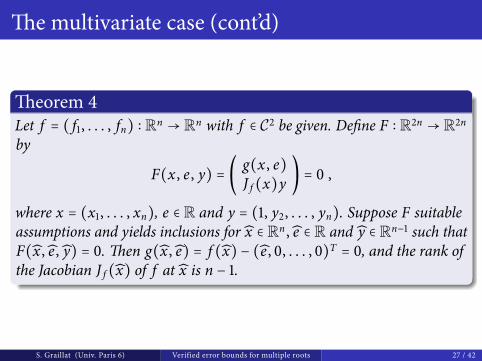
heorem 4Let f = ( f1, . . . , fn) ∶ Rn → Rn with f ∈ C2 be given. Deûne F ∶ R2n → R2n
by
F(x , e , y) = ( g(x , e)J f (x)y
) = 0 ,
where x = (x1, . . . , xn), e ∈ R and y = (1, y2, . . . , yn). Suppose F suitableassumptions and yields inclusions for x ∈ Rn , e ∈ R and y ∈ Rn−1 such thatF(x , e , y) = 0. hen g(x , e) = f (x) − (e , 0, . . . , 0)T = 0, and the rank ofthe Jacobian J f (x) of f at x is n − 1.
S. Graillat (Univ. Paris 6) Verified error bounds for multiple roots 27 / 42
hemultivariate case (cont’d)
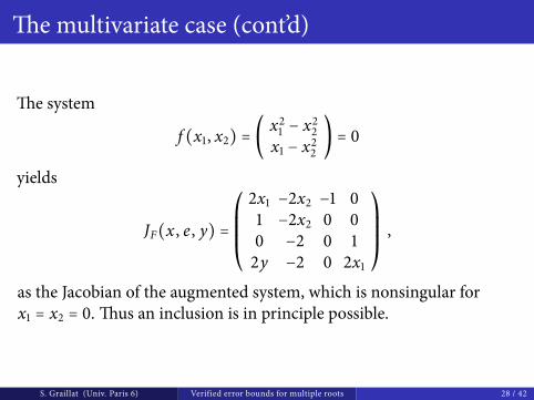
he system
f (x1, x2) = ( x21 − x2
2x1 − x2
2) = 0
yields
JF(x , e , y) =⎛⎜⎜⎜⎝
2x1 −2x2 −1 01 −2x2 0 00 −2 0 12y −2 0 2x1
⎞⎟⎟⎟⎠,
as the Jacobian of the augmented system, which is nonsingular forx1 = x2 = 0. hus an inclusion is in principle possible.
S. Graillat (Univ. Paris 6) Verified error bounds for multiple roots 28 / 42
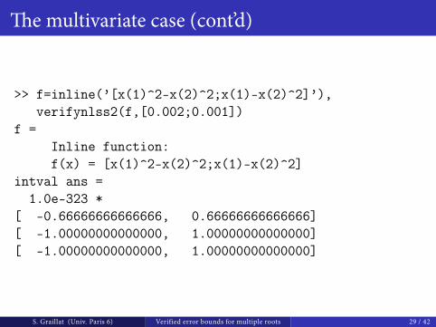
hemultivariate case (cont’d)
>> f=inline(’[x(1)^2-x(2)^2;x(1)-x(2)^2]’),verifynlss2(f,[0.002;0.001])
f =Inline function:f(x) = [x(1)^2-x(2)^2;x(1)-x(2)^2]
intval ans =1.0e-323 *
[ -0.66666666666666, 0.66666666666666][ -1.00000000000000, 1.00000000000000][ -1.00000000000000, 1.00000000000000]
S. Graillat (Univ. Paris 6) Verified error bounds for multiple roots 29 / 42
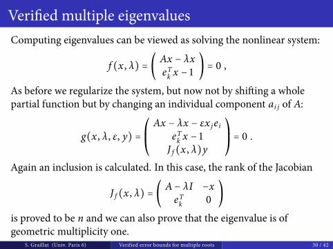
Veriûedmultiple eigenvaluesComputing eigenvalues can be viewed as solving the nonlinear system:
f (x , λ) = ( Ax − λxeTk x − 1 ) = 0 ,
As before we regularize the system, but now not by shi�ing a wholepartial function but by changing an individual component ai j of A:
g(x , λ, ε, y) =⎛⎜⎝
Ax − λx − εx jeieTk x − 1
J f (x , λ)y
⎞⎟⎠= 0 .
Again an inclusion is calculated. In this case, the rank of the Jacobian
J f (x , λ) = ( A− λI −xeTk 0 )
is proved to be n and we can also prove that the eigenvalue is ofgeometricmultiplicity one.
S. Graillat (Univ. Paris 6) Verified error bounds for multiple roots 30 / 42

Outline of the talk
1 Principle of self-validating methods
2 Multiple roots of polynomial systems
3 Numerical experiments
S. Graillat (Univ. Paris 6) Verified error bounds for multiple roots 31 / 42
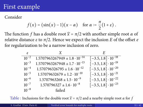
First exampleConsider
f (x) = (sin(x) − 1)(x − α) for α ∶= π2(1 + ε) .
he function f has a double root x = π/2 with another simple root α ofrelative distance ε to π/2. Hence we expect the inclusion E of the oòset efor regularization to be a narrow inclusion of zero.
ε X E10−2 1.5707963267949 ± 1.8 ⋅ 10−14 [−3.5, 1.8] ⋅ 10−18
10−3 1.5707963267948 ± 1.7 ⋅ 10−13 [−3.5, 1.8] ⋅ 10−19
10−4 1.570796326795 ± 1.6 ⋅ 10−12 [−3.5, 1.8] ⋅ 10−20
10−5 1.57079632679 ± 1.2 ⋅ 10−10 [−3.5, 1.8] ⋅ 10−21
10−6 1.5707963268 ± 1.5 ⋅ 10−9 [−3.5, 1.8] ⋅ 10−22
10−7 1.570796327 ± 1.6 ⋅ 10−8 [−3.5, 1.8] ⋅ 10−23
10−8 failed
Table : Inclusions for the double root x = π/2 and a nearby simple root α for f
S. Graillat (Univ. Paris 6) Verified error bounds for multiple roots 32 / 42
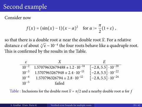
Second exampleConsider now
f (x) = (sin(x) − 1)(x − α)2 for α ∶= π2(1 + ε) ,
so that there is a double root α near the double root x. For a relativedistance ε of about 4
√ε ∼ 10−4 the four roots behave like a quadruple root.
his is conûrmed by the results in the Table.
ε X E10−2 1.57079632679488 ± 1.2 ⋅ 10−14 [−2.8, 5.5] ⋅ 10−20
10−3 1.5707963267948 ± 2.4 ⋅ 10−13 [−2.8, 5.5] ⋅ 10−22
10−4 1.570796326794 ± 2.8 ⋅ 10−12 [−2.8, 5.5] ⋅ 10−24
10−5 failed
Table : Inclusions for the double root x = π/2 and a nearby double root α for f
S. Graillat (Univ. Paris 6) Verified error bounds for multiple roots 33 / 42
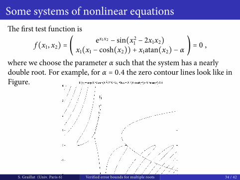
Some systems of nonlinear equationshe ûrst test function is
f (x1, x2) = ( ex1x2 − sin(x21 − 2x1x2)
x1(x1 − cosh(x2)) + x1atan(x2) − α) = 0 ,
where we choose the parameter α such that the system has a nearlydouble root. For example, for α = 0.4 the zero contour lines look like inFigure.
S. Graillat (Univ. Paris 6) Verified error bounds for multiple roots 34 / 42
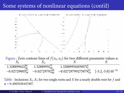
Some systems of nonlinear equations (cont’d)
Figure : Zero contour lines of f (x1, x2) for two diòerent parameter values α.X1 X2 X E
1.3288996218628 1.328899515748 1.3288995683907165−0.027298056759 −0.0272979298
88 −0.027297992758794134 [-5.2,-5.0]⋅10−14
Table : Inclusions X1 , X2 for two single roots and X for a nearly double root for f andα = 0.4003120447407.
S. Graillat (Univ. Paris 6) Verified error bounds for multiple roots 35 / 42
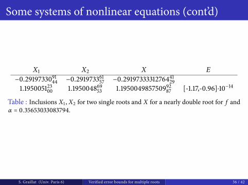
Some systems of nonlinear equations (cont’d)
X1 X2 X E−0.2919733091
44 −0.29197336157 −0.2919733331276441
291.19500512300 1.19500486953 1.195004985750992
87 [-1.17,-0.96]⋅10−14
Table : Inclusions X1 , X2 for two single roots and X for a nearly double root for f andα = 0.35653033083794.
S. Graillat (Univ. Paris 6) Verified error bounds for multiple roots 36 / 42
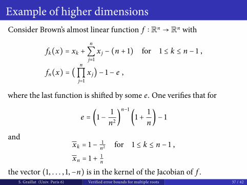
Example of higher dimensionsConsider Brown’s almost linear function f ∶ Rn → Rn with
fk(x) = xk +n
∑j=1
x j − (n + 1) for 1 ≤ k ≤ n − 1 ,
fn(x) = (n
∏j=1
x j) − 1 − e ,
where the last function is shi�ed by some e. One veriûes that for
e = (1 − 1n2)
n−1(1 + 1
n) − 1
andxk = 1 − 1
n2 for 1 ≤ k ≤ n − 1 ,
xn = 1 + 1n
the vector (1, . . . , 1,−n) is in the kernel of the Jacobian of f .S. Graillat (Univ. Paris 6) Verified error bounds for multiple roots 37 / 42
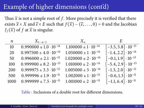
Example of higher dimensions (cont’d)hus x is not a simple root of f . More precisely it is veriûed that thereexists x ∈ X and ε ∈ E such that f (x) − (ε, . . . , 0) = 0 and the JacobianJ f (x) of f at x is singular.
n X1⋯n−1 Xn E10 0.990000 ± 1.0 ⋅ 10−14 1.100000 ± 1 ⋅ 10−14 [−3.5, 5.8] ⋅ 10−1520 0.997500 ± 4.0 ⋅ 10−14 1.050000 ± 1 ⋅ 10−14 [−1.4, 2.2] ⋅ 10−1450 0.996000 ± 2.1 ⋅ 10−13 1.020000 ± 2 ⋅ 10−14 [−0.1, 1.9] ⋅ 10−13100 0.999900 ± 8.2 ⋅ 10−13 1.010000 ± 2 ⋅ 10−14 [−5.4, 2.9] ⋅ 10−13200 0.999975 ± 3.3 ⋅ 10−12 1.005000 ± 5 ⋅ 10−14 [−1.3, 2.0] ⋅ 10−12500 0.999996 ± 1.9 ⋅ 10−11 1.002000 ± 1 ⋅ 10−13 [−0.6, 1.3] ⋅ 10−111000 0.999999 ± 7.5 ⋅ 10−11 1.001000 ± 2 ⋅ 10−13 [−1.1, 6.4] ⋅ 10−11
Table : Inclusions of a double root for diòerent dimensions.
S. Graillat (Univ. Paris 6) Verified error bounds for multiple roots 38 / 42
Conclusion and future work
Conclusion:Eõcient algorithms for computing veriûed and narrow errorbounds with the property that a slightly perturbed system is provedto have a double root within the computed boundsApplied those to univariate polynomials, to multivariatepolynomials and also to eigenvalue problemsNumerical experiments have conûrmed the performance of ouralgorithms
Future work:Detecting singular matricesApplications to approximate coprimeness
S. Graillat (Univ. Paris 6) Verified error bounds for multiple roots 39 / 42
Bibliography I
SiegfriedM. Rump and Stef Graillat.Veriûed error bounds for multiple roots of systems of nonlinearequations.Numer. Algorithms, 54 (2010), no. 3, 359-377.
SiegfriedM. Rump.Veriûcation methods: Rigorous results using �oating-pointarithmetic.Acta Numerica (2010), pp. 287-449.
Bo Einarsson.Accuracy and Reliability in Scientiûc Computing.So�ware-Environments-Tools. SIAM, Philadelphia, PA, 2005.
S. Graillat (Univ. Paris 6) Verified error bounds for multiple roots 40 / 42

Bibliography II
Nicholas J. Higham.Accuracy and stability of numerical algorithms.Society for Industrial and AppliedMathematics (SIAM),Philadelphia, PA, second edition, 2002.
Jean-Michel Muller et al.Handbook of Floating-Point Arithmetic.Birkhäuser, 2010.
R. Moore, R. Kearfott et M. Cloud.Introduction to Interval Analysis.SIAM, 2009.
S. Graillat (Univ. Paris 6) Verified error bounds for multiple roots 41 / 42

hank you for your attention
S. Graillat (Univ. Paris 6) Verified error bounds for multiple roots 42 / 42