TALLINN UNIVERSITY OF TECHNOLOGY

Faculty of Information Technology

Department of Computer Engineering

Tallinn 2015

IAG70LT

Erik Kaju 132643IASM

DECISION SUPPORT SYSTEM FOR FINANCIAL LIQUIDITY PLANNING

Master’s Thesis

Supervisor:

Tarmo Robal (PhD) Research Scientist

Consultants:

Eero Ringmäe Payment Processing expert

Lauri Hein Payment Processing expert

2

Author’s declaration of originality

I hereby certify that I am the sole author of this thesis. All the used materials, references to the

literature and the work of others have been referred to. This thesis has not been presented for

examination anywhere else.

Author: Erik Kaju

31.05.15

3

Abstract

The objective of this thesis is to use information technology facilities and build a minimum

viable product solution that would potentially enhance a liquidity planning process in the

world’s fastest growing money transfer service. Liquidity, in context of this thesis, is a

sufficient amount of monetary funds on remittance company’s foreign bank account. The goal is

to build a prototype of decision support system for making liquidity balancing decisions based

on historical data of fund flows. System must be able to forecast future transfer volumes and

propose when it is the right time to buy certain currency and how much company should buy

that. If the company handled in this thesis shifts too much liquidity to its foreign account, then it

is an unreasonable expense of resources and exchange rate risk (FX risk). If the company shifts

too little liquidity, then it cannot deliver its core business – perform international money

transfers in promised time. The difficulty of forecasting lies in the fact of rapidly changing

environment, randomness and, most of all, diversity of factors that influence the demand for

money. These factors need to be analysed and included in the computational model of MVP.

The prototype will focus only on one specific remittance route – the author of this thesis chose

the remittance channel to Indian rupee. Solution will be tested with real historical data and,

based on the results, author will asseverate whether the proposed model is credible and further

enhancement of the solution is reasonable and encouraged.

This thesis is written in English and is 63 pages long, including 6 chapters, 33 figures and 12

tables.

4

Annotatsioon

Finantslikviidsuse planeerimise otsustusabi süsteem

Antud magistritöö eesmärgiks on otsustusabi süsteemi prototüübi loomine, mis aitaks

potentsiaalselt parendada likviidsuse planeerimise protsessi maailma kiireima kasvuga

rahaülekannete teenust pakkuvas ettevõttes. Käesoleva magistritöö kontekstis tähendab

likviidsus eelkõige väljamakseteks piisavate rahaliste vahendite olemasolu ettevõtte välisvaluuta

kontol. Eesmärgiks on luua otsustusabi süsteemi prototüüp, mis tugineks rahavoogude

statistilistele andmetele ning ennustaks tuleviku rahaülekannete mahtu. Ennustuste ja ettevõtte

kontoseisude analüüsi põhjal peab süsteem tegema põhjendatud ettepanekuid, millal ning mis

koguses peaks ostma välisvaluutat. Kui magistritöös käsitletav ettevõte saadab väliskontole liiga

palju rahalist ressurssi, siis on see omavahendite kulu ning valuutarisk. Kui ettevõte saadab liiga

vähe, siis ei suudeta pakkuda klientidele stabiilset põhiteenust – rahvusvahelisi rahaülekandeid

lubatud ajalistes raamides. Rahavoogude ennustamise keerukuseks on kiiresti muutuv keskkond,

juhuslikkus ja raha vajadust mõjutavate faktorite paljusus. Need faktorid tuleb läbi analüüsida

ning lisada loodava prototüübi arvutusmudelisse. Magistritöö käigus loodav prototüüp

keskendub ainult ühele rahaülekannete marsruudile, autor valis selleks rahaülekanded India

ruupiatesse. Lahendust testitakse reaalsete ajalooliste andmetega, ning tuginedes katsete

tulemustele antakse hinnang, kas väljapakutud arvutusmudelil on potentsiaali ning, kas

lahenduse edaspidine arendus on mõistlik ja õigustatud.

Lõputöö on kirjutatud inglise keeles ning sisaldab teksti 63 leheküljel, 6 peatükki, 33 joonist, 12

tabelit.

5

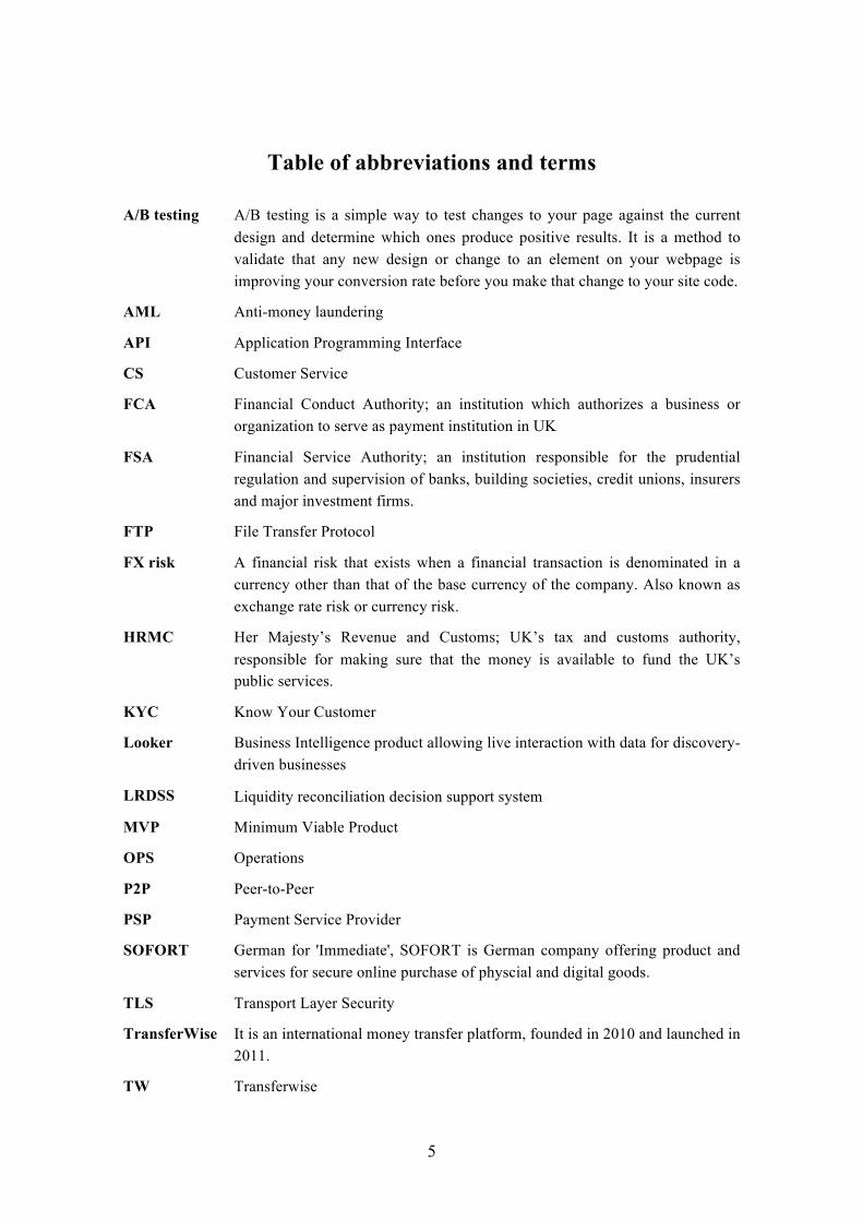
Table of abbreviations and terms

A/B testing   A/B testing is a simple way to test changes to your page against the current design and determine which ones produce positive results. It is a method to validate that any new design or change to an element on your webpage is improving your conversion rate before you make that change to your site code.  

AML   Anti-money laundering

API   Application Programming Interface

CS   Customer Service

FCA   Financial Conduct Authority; an institution which authorizes a business or organization to serve as payment institution in UK

FSA   Financial Service Authority; an institution responsible for the prudential regulation and supervision of banks, building societies, credit unions, insurers and major investment firms.  

FTP   File Transfer Protocol

FX risk   A financial risk that exists when a financial transaction is denominated in a currency other than that of the base currency of the company. Also known as exchange rate risk or currency risk.

HRMC   Her Majesty’s Revenue and Customs; UK’s tax and customs authority, responsible for making sure that the money is available to fund the UK’s public services.

KYC   Know Your Customer

Looker   Business Intelligence product allowing live interaction with data for discovery-driven businesses  

LRDSS Liquidity reconciliation decision support system

MVP   Minimum Viable Product

OPS   Operations

P2P   Peer-to-Peer

PSP Payment Service Provider

SOFORT German for 'Immediate', SOFORT is German company offering product and services for secure online purchase of physcial and digital goods.

TLS Transport Layer Security

TransferWise It is an international money transfer platform, founded in 2010 and launched in 2011.

TW Transferwise

6

Table of contents

1.   Introduction ............................................................................................................. 11  

2.   Business overview - TransferWise .......................................................................... 14  

2.1.   Customer experience ........................................................................................ 14  

2.2.   P2P money transfers ......................................................................................... 15  

2.3.   Safety and privacy ............................................................................................ 16  

2.4.   Business specific financial operations .............................................................. 17  

2.5.   Liquidity balances reconciliation planning – the problem explained ............... 19  

2.6.   Detailed objective of this thesis ........................................................................ 20  

3.   Liquidity planning: analysis of factors .................................................................... 22  

3.1.   Time-series analysis ......................................................................................... 22  

3.1.1.   Time-series ................................................................................................ 22  

3.1.2.   Sample size ................................................................................................ 23  

3.2.   External factors ................................................................................................. 24  

3.2.1.   Recent volume descriptor .......................................................................... 24  

3.2.2.   Growth trends ............................................................................................ 25  

3.2.3.   Weekly patterns ......................................................................................... 28  

3.2.4.   Monthly patterns ........................................................................................ 29  

3.2.5.   Exchange rate movements ......................................................................... 30  

3.2.6.   Frequency of extra large payment orders .................................................. 31  

3.2.7.   National Holidays ...................................................................................... 32  

3.3.   Internal factors .................................................................................................. 33  

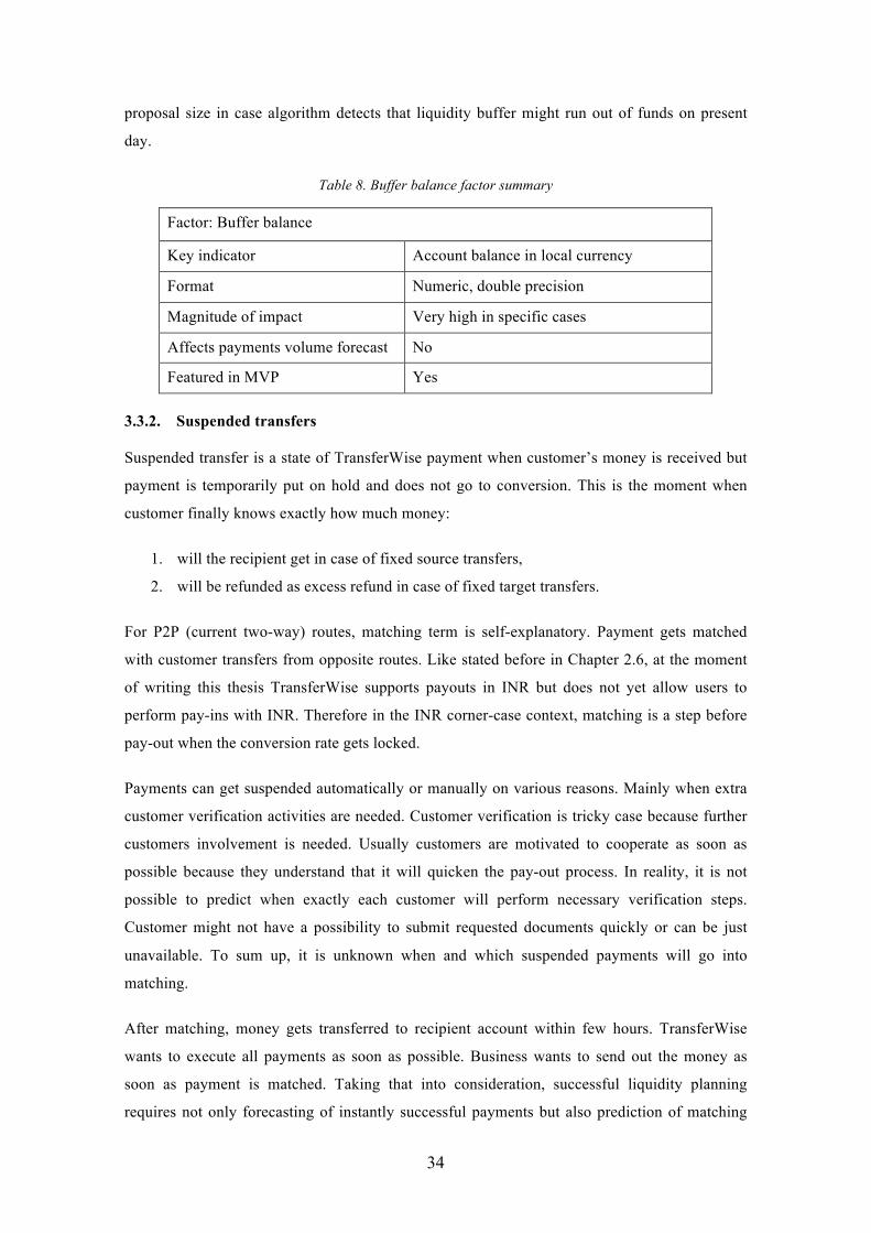
3.3.1.   Liquidity buffer account balance ............................................................... 33  

3.3.2.   Suspended transfers ................................................................................... 34  

3.3.3.   Liquidity in transit ..................................................................................... 35  

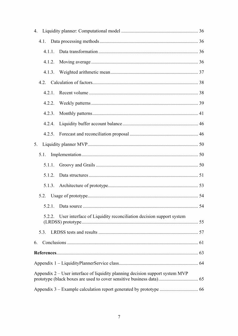
7

4.   Liquidity planner: Computational model ................................................................ 36  

4.1.   Data processing methods .................................................................................. 36  

4.1.1.   Data transformation ................................................................................... 36  

4.1.2.   Moving average ......................................................................................... 36  

4.1.3.   Weighted arithmetic mean ......................................................................... 37  

4.2.   Calculation of factors ........................................................................................ 38  

4.2.1.   Recent volume ........................................................................................... 38  

4.2.2.   Weekly patterns ......................................................................................... 39  

4.2.3.   Monthly patterns ........................................................................................ 41  

4.2.4.   Liquidity buffer account balance ............................................................... 46  

4.2.5.   Forecast and reconciliation proposal ......................................................... 46  

5.   Liquidity planner MVP ............................................................................................ 50  

5.1.   Implementation ................................................................................................. 50  

5.1.1.   Groovy and Grails ..................................................................................... 50  

5.1.2.   Data structures ........................................................................................... 51  

5.1.3.   Architecture of prototype ........................................................................... 53  

5.2.   Usage of prototype ............................................................................................ 54  

5.2.1.   Data source ................................................................................................ 54  

5.2.2.   User interface of Liquidity reconciliation decision support system (LRDSS) prototype ................................................................................................. 55  

5.3.   LRDSS tests and results ................................................................................... 57  

6.   Conclusions ............................................................................................................. 61  

References ...................................................................................................................... 63  

Appendix 1 – LiquidityPlannerService class .................................................................. 64  

Appendix 2 – User interface of liquidity planning decision support system MVP prototype (black boxes are used to cover sensitive business data) ................................. 65  

Appendix 3 – Example calculation report generated by prototype ................................ 66  

8

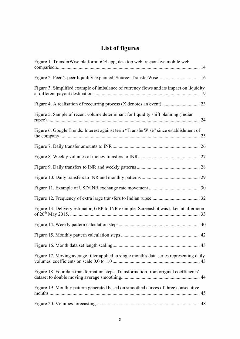
List of figures

Figure 1. TransferWise platform: iOS app, desktop web, responsive mobile web comparison ...................................................................................................................... 14  

Figure 2. Peer-2-peer liquidity explained. Source: TransferWise .................................. 16  

Figure 3. Simplified example of imbalance of currency flows and its impact on liquidity at different payout destinations ....................................................................................... 19  

Figure 4. A realisation of reccurring process (X denotes an event) ............................... 23  

Figure 5. Sample of recent volume determinant for liquidity shift planning (Indian rupee) .............................................................................................................................. 24  

Figure 6. Google Trends: Interest against term “TransferWise” since establishment of the company .................................................................................................................... 25  

Figure 7. Daily transfer amounts to INR ........................................................................ 26  

Figure 8. Weekly volumes of money transfers to INR ................................................... 27  

Figure 9. Daily transfers to INR and weekly patterns .................................................... 28  

Figure 10. Daily transfers to INR and monthly patterns ................................................ 29  

Figure 11. Example of USD/INR exchange rate movement .......................................... 30  

Figure 12. Frequency of extra large transfers to Indian rupee ........................................ 32  

Figure 13. Delivery estimator, GBP to INR example. Screenshot was taken at afternoon of 20th May 2015. ........................................................................................................... 33  

Figure 14. Weekly pattern calculation steps ................................................................... 40  

Figure 15. Monthly pattern calculation steps ................................................................. 42  

Figure 16. Month data set length scaling ........................................................................ 43  

Figure 17. Moving average filter applied to single month's data series representing daily volumes' coefficients on scale 0.0 to 1.0 ........................................................................ 43  

Figure 18. Four data transformation steps. Transformation from original coefficients’ dataset to double moving average smoothing ................................................................. 44  

Figure 19. Monthly pattern generated based on smoothed curves of three consecutive months ............................................................................................................................ 45  

Figure 20. Volumes forecasting ...................................................................................... 48  

9

Figure 21. SingleDayData class ...................................................................................... 51  

Figure 22. WeekData class ............................................................................................. 52  

Figure 23. WeekSummary class ..................................................................................... 52  

Figure 24. MonthData class ............................................................................................ 53  

Figure 25. Abstracted visualisation of MVP prototype architecture .............................. 53  

Figure 26. Daily volumes time series data export from Looker ..................................... 54  

Figure 27. Data import in prototype ............................................................................... 55  

Figure 28. Simulation day selection in prototype ........................................................... 55  

Figure 29. Recent volume settings in prototype ............................................................. 55  

Figure 30. Weekly patterns settings in prototype ........................................................... 56  

Figure 31. Monthly patterns settings in prototype .......................................................... 56  

Figure 32. Forecast section and payout simulation in prototype (black boxes are used to cover sensitive business data) ......................................................................................... 56  

Figure 33. Liquidity shift proposal in prototype (black boxes are used to cover sensitive business data) .................................................................................................................. 57  

10

List of tables

Table 1. Recent volume factor summary ........................................................................ 24  

Table 2. Growth of volume factor summary .................................................................. 27  

Table 3. Weekly patterns factor summary ...................................................................... 29  

Table 4. Monthly patterns factor summary .................................................................... 30  

Table 5. Exchange rate movement factor summary ....................................................... 31  

Table 6. Frequency of large payments factor summary ................................................. 32  

Table 7. National holidays factor summary .................................................................... 33  

Table 8. Buffer balance factor summary ........................................................................ 34  

Table 9. Suspended transfers factor summary ................................................................ 35  

Table 10. Liquidity in transit factor summary ................................................................ 35  

Table 11. Test scenario matrix table ............................................................................... 59  

Table 12. Test execution results ..................................................................................... 59  

11

1. Introduction

Traditionally, for businesses, cash in form of physical banknotes or money in a bank account,

fulfils an operational function, and is used to buy the resources that the business needs.

However, monetary funds is also a resource in itself, and as such has a value or cost measurable

as interest. To an operations manager, cash is something that is not kept for its own sake, but is

needed by the business to carry out its activities. The reasons for holding monetary means,

therefore, are to pay for purchased items and to provide contingency funding should an

unexpected spending need arise. Companies might use the funds to buy raw materials or pay off

the production costs. Liquidity is needed to meet this operational demand for cash [1].

Cash is also subject to shrinkage in value because of inflation that is an inevitable financial risk.

So there is always a need to control monetary funds and keep non-interest earning balances as

low as safely possible. The role of cash management is to plan, monitor and control the cash

flows and the cash position of the company, maintaining its liquidity. The classical meaning of

liquidity is the ability to mobilise cash for the purchase of assets or to cover actual or potential

liabilities. The demand for liquidity is motivated by the need to pay for expenditures, the wish

to take advantage of opportunities that might arise and the need to avoid financial distress [1].

Liquidity analysis requires the use of budgets, particularly the cash budget, which forecasts cash

flows in future periods [2].

One essential challenge of efficient cash management is the forecasting of cash deficits. Cash

forecasting is vital to ensure that sufficient funds are available when they are needed at an

acceptable cost. Forecasts provide an early warning of liquidity problems by estimating how

much, when, how long the cash is required and whether it will be available from anticipated

sources. The price of liquidity is interest, plus arrangement fees for borrowing and other costs

such as legal fees [1].

Above-cited characterisation describes the essence of cash management and liquidity in

traditional established businesses like manufacturing, retail trading and other paid services

where, from end customer point of view, the money is exchanged for goods or services.

In money remittance business, several of above mentioned distinct terms almost conflate into

one. Customers pay in cash for the service of transferring the cash and the commodity that they

buy is also in a form of cash. In international remittance where we are dealing with cross-

exchange transfers, customers buy a cash of foreign currency. Of course in remittance the

classical concept of liquidity still takes place. Money in company’s own bank account fulfils

12

businesses operational needs. Remittance company does not manufacture goods, but for

instance, all financial operations accompanying the remittance and currency exchange service

have own net costs. It is the best practice, and in many cases a requirement from financial

authorities, that customers’ money is set aside in a separate accounts from businesses ones [3].

That is especially vivid in peer-to-peer remittance model (described in details in Chapter 2.2)

where the ultimate goal is to match customer’s money in different destinations in real time.

Precautionary store of funds in accounts located at each possible destination of remittance

channels is a form of liquidity too. Technically, the funds in these accounts belong to customers,

all traditional liquidity risks are also in effect and business is responsible for efficient

management. In this case liquidity means having enough cash to settle pay-out transactions on

the due date. In case of multi-currency remittance the cash in pay-out bank accounts is subject

to shrinkage in value because of (in addition to plain inflation) possible adverse exchange rate

movements. At any point, there are always exchange markets that are less stable than others. So

unreasonable accumulation of surplus funds might cause financial loss. On the other hand, funds

deficit may result in delays of remittance payouts which for instant money transfer business is a

critical case.

The objective of this thesis is to use information technology facilities to build a minimum viable

product (MVP) [4] solution that would potentially enhance a liquidity planning process in the

world’s fastest growing money transfer service. According to Eric Ries, a MVP is such version

of a new product which allows to collect the maximum amount of validated learning with the

least effort [4]. The goal is to build a prototype of decision support system for making liquidity

balancing decisions based on historical data of fund flows. The system must forecast future

transfer volumes in future and propose when it is the right time to buy certain currency and how

much company should buy it. If company shifts too much liquidity to foreign account, it is an

unreasonable expense of resources and FX risk. If company shifts too little liquidity, then it

cannot deliver its core business. The difficulty of forecasting lies in the fact of diversity of

factors that influence the demand for money, rapidly changing environment and randomness.

This prototype will focus only on one specific remittance route. The author chose the remittance

channel to Indian rupee (INR). Remittance route to INR is among the fastest growing ones and

liquidity shift takes long time. From perspective of liquidity management, INR requires much

attention and potential mistakes are costly. Solution will be tested with real historical data and

based on the results author will asseverate whether the proposed model is credible and further

enhancement of the solution is reasonable and encouraged.

To start with, Chapter 2 gives an overview about remittance company this thesis is based on.

That chapter specifies characteristic working principles, roles, processes – necessary

13

background information for in-depth understanding of the problem. Then detailed explanation

of the challenge and elaborated objective of the thesis are expounded. Next, in Chapter 3, comes

the analysis of various factors that are underlying determinants regarding the problem. In

Chapter 4, author will proceed with explication of computational model. That chapter describes

how indications from selected problem factors are used to calculate the forecast. Further on,

Chapter 5 is focused on the MVP implementation – how computational model is realised, which

data structures used, the usage of the prototype, applied testing approaches and summary of the

results. Last, Chapter 6 will summarise the outcome of the thesis.

14

2. Business overview - TransferWise

TransferWise (TW) is an international money transfer platform. It makes it up to 10 times

cheaper to send money abroad compared to using similar services offered by banks. Developed

by the people who built Skype and PayPal, it uses peer-to-peer technology to get rid of all the

fees banks and brokers have kept hidden for decades.

International money transfers are more expensive than meets the eye. Although banks and

brokers often claim there are ‘no fees’, many take as much as 5 percent of the money being sent.

Customers have already moved more than £4,5bn using the platform - an approach that has

saved them £180m [5].

2.1. Customer experience

TransferWise platform is available in web browser, both desktop or mobile-friendly web. User

experience and convenience are strongly emphasised. There are also native applications for

Android and iOS devices. Company aims at creating the best financial service for its customers

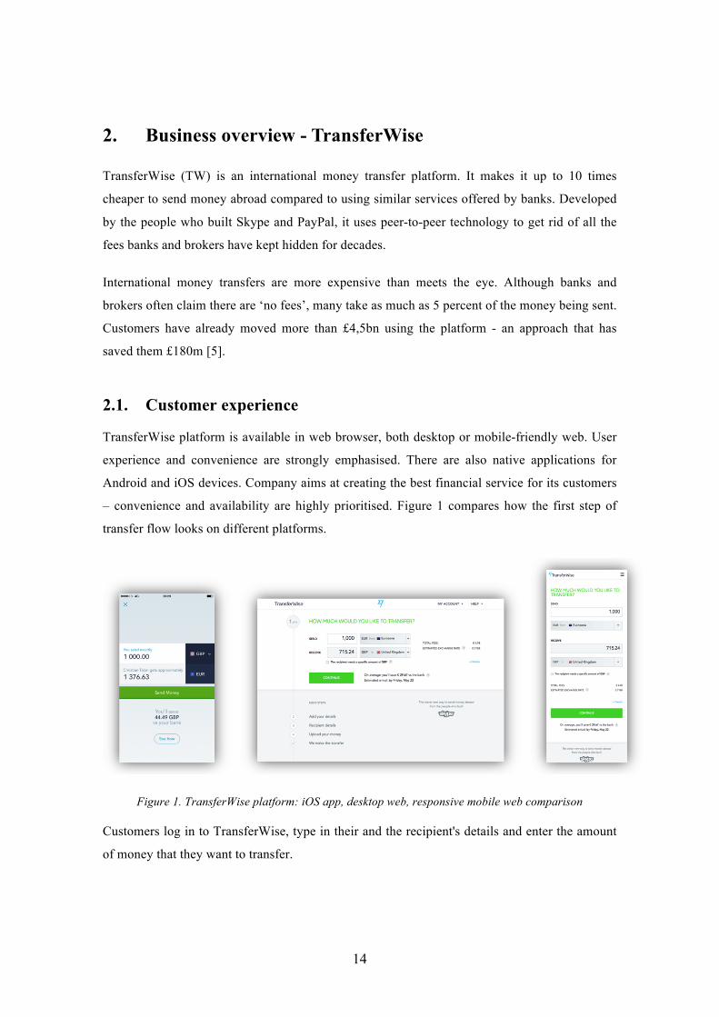
– convenience and availability are highly prioritised. Figure 1 compares how the first step of

transfer flow looks on different platforms.

Figure 1. TransferWise platform: iOS app, desktop web, responsive mobile web comparison

Customers log in to TransferWise, type in their and the recipient's details and enter the amount

of money that they want to transfer.

15

User has a payment option choice:

§ to type in debit card details,

§ go on to internet banking and send the money to TransferWise account,

§ use alternative payment methods, for instance, SOFORT in Europe.

Customer will receive a confirmation email when TW has received the money and another one

when it has been paid out to the recipient.

Costs, speed and convenience are ground for customer motivation. TransferWise never hides its

fees in the exchange rate like it is done by banks or brokers. It clearly presents all its costs

upfront before the customer makes a transfer. Costs vary between currencies, but each route is

typically 10 times cheaper than the average high street bank. The system is based on free or

extremely low-cost local transfers, so the banks have no opportunity to charge their extortionate

fees. The aim of TW is to offer instant T+0 transfers. Ideally, the whole transaction should be

complete within the same day – significantly faster than using a bank. For instance an

international bank transfer of $200 from the US to China, Mexico or Philippines can take up to

5 days and transaction cost will be approximately 6,5% (versus 0,5% in TW) [6].

TransferWise supports money transfers between euro, British pound, Swiss franc, Polish zloty,

Turkish lira, Romania leu, Bulgarian lev, Georgian lari, Hungarian forint, Danish, Swedish,

Czech, Norwegian krone, Australian, Canadian and US dollar. It also supports transfers from

above mentioned currencies to Indian rupee, Malaysian ringgit, Singaporean, Hong Kong, and

New Zealand dollar. Transfers from these to all other supported currencies and many other

routes are continuously added. TW plans to cover all the key markets by the end of 2015.

2.2. P2P money transfers

The technology behind TransferWise is based on a peer-to-peer system. If someone wants to

convert their pounds to euros, TransferWise finds someone who wants to transfer money in the

opposite direction (in this example euros into pounds). The system automatically matches the

currency flows at the real mid-market exchange rate and then pays out from the local euro or

pound account, meaning the money never actually moves across borders. Doing things this way

means customers can avoid traditional banking fees altogether.

Some of currency routes are directly peer-to-peer. This means TransferWise matches customers’

money moving in one direction with another customer’s funds being transferred in the opposite.

It is done on popular, established routes such as euro and pound sterling, for instance. Figure 2

describes the principle of P2P international remittance.

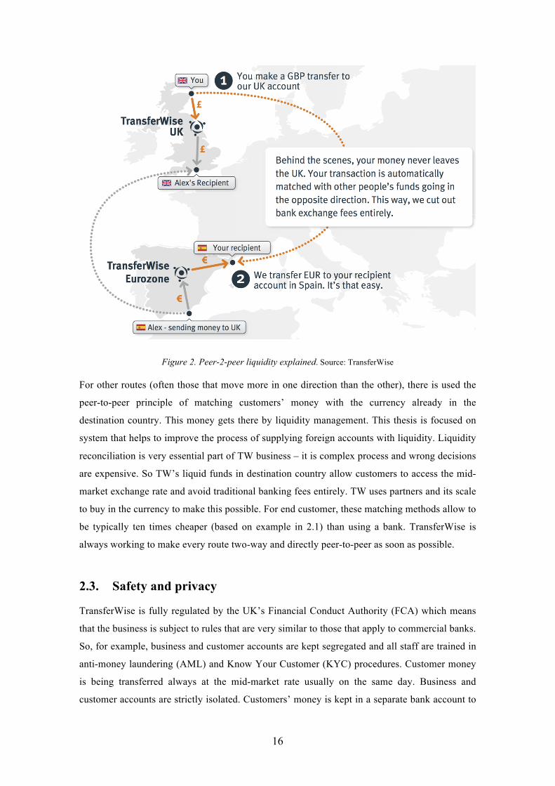
16

Figure 2. Peer-2-peer liquidity explained. Source: TransferWise

For other routes (often those that move more in one direction than the other), there is used the

peer-to-peer principle of matching customers’ money with the currency already in the

destination country. This money gets there by liquidity management. This thesis is focused on

system that helps to improve the process of supplying foreign accounts with liquidity. Liquidity

reconciliation is very essential part of TW business – it is complex process and wrong decisions

are expensive. So TW’s liquid funds in destination country allow customers to access the mid-

market exchange rate and avoid traditional banking fees entirely. TW uses partners and its scale

to buy in the currency to make this possible. For end customer, these matching methods allow to

be typically ten times cheaper (based on example in 2.1) than using a bank. TransferWise is

always working to make every route two-way and directly peer-to-peer as soon as possible.

2.3. Safety and privacy

TransferWise is fully regulated by the UK’s Financial Conduct Authority (FCA) which means

that the business is subject to rules that are very similar to those that apply to commercial banks.

So, for example, business and customer accounts are kept segregated and all staff are trained in

anti-money laundering (AML) and Know Your Customer (KYC) procedures. Customer money

is being transferred always at the mid-market rate usually on the same day. Business and

customer accounts are strictly isolated. Customers’ money is kept in a separate bank account to

17

the businesses as required by the Financial Conduct Authority (FCA). The platform is also very

well capitalised (received $25m worth of investment from Sir Richard Branson and Peter Thiel,

the co-founder of PayPal and later $58m from Ben Horowitz and Marc Andreessen) [7, 8, 9].

TransferWise meets all legal requirements placed on it by the Financial Conduct Authority

(FCA), HM Revenue & Customs (HMRC) and its banking partners to prevent money

laundering – particularly in regards to each Government’s KYC procedures where TransferWise

operates. These regulations require businesses to know, understand and be able to prove the

identity of all their customers in order to quickly close down the account of anyone suspected of

involvement in illegal activities. TransferWise ensures this is done to a high standard by giving

regular training to all its staff. While no financial business can ever be 100 percent certain that

they are not being used for illegal activity, TransferWise takes a number of additional steps,

such as employing a third party advisor, to inform and monitor its anti-money laundering

procedures. [7] [8] [9]

Customer data is kept securely within the terms of the Data Protection Act [10]. The

Information Commissioner's Office has registered TransferWise under the Data Protection Act

98 [11]. Protecting customers and their data is important for the company. No personal data is

ever shared with third parties unless required so by law. Communication of sensitive

information between customer’s browser and TransferWise servers is encrypted using Transport

Layer Security (TLS) [12].

2.4. Business specific financial operations

To assure seamless functioning of the business, several different teams operate in TransferWise.

In context of this thesis, it is worth mentioning Operations (OPS). It is one of the core teams of

the business. OPS experts process all payments from end-to-end, solve any problems and

obstacles on the way. The aim is to process all payments with high speed and quality which

gives direct input to customer satisfaction. This team is in charge for liquidity management

(LM). LM role decides every morning on a daily basis how much and where to shift liquidity.

There are several business specific financial operations and concomitant events that are

involved in the TransferWise model. These operations are as follows:

§ deposit receipt,

§ payment execution,

§ fees reconciliation,

§ liquidity.

18

The majority of these actions are performed automatically. Operations specialists monitor

automated processes via dedicated interface continuously every day. Human interactions are

needed when system detects mistakes. It happens mostly when users enter incorrect details.

Responsible ops agents are informed about incidents automatically and correct the invalid data,

if possible. If necessary, the customer support contacts the sender to correct the details.

Deposit receipt (pay-in) is the first link in chain of TW money transferring operations. At first,

an internal customer payment order gets registered in TW system. Customers send their deposits

via bank transfer to TransferWise’s account in partner bank. TW receives bank statements

automatically and then system links transactions from received statement with internal customer

payment orders and reconciles them. For card payments the principle is the same but instead of

partner bank, there is a card payment processing partner, often referred as payment service

provider (PSP).

Payment execution (pay-out) is the most pleasant operation for end user because the money gets

paid out on the other end. TW prepares payments batch in system and then imparts the payment

file to partner’s payment system (the banking partner that performs a pay-out to the desired

account). Generally, payment submissions are successful – in case of problems TW resolves

rejection reasons and re-submits the payment. Customer gets notified via email that payment

has been successfully processed and partner bank sends out the money. As it is a local transfer,

it never takes more than a few hours. For end user the process has finished – simple and fast.

The interaction between bank and TransferWise goes on – bank statement containing executed

pay-outs gets automatically imported into system. TW links transactions in statement with

customer payment orders and reconciles the data.

Liquidity related operations are also of special character. Successful liquidity management

guarantees that liquidity buffers are always optimally balanced and there is always enough

money for payouts. Liquidity is the main focus of current thesis.

There are two different options how TransferWise manages to replenish liquidity buffers:

§ transfer funds in foreign currency to designated account,

§ transfer funds in local currency to designated account.

In case of foreign currency, TW exchanges the foreign currency to local one with partner’s

trading team. Thereafter, the partner credits the fund in local currency to TW designated

account. Consequent process is already familiar from deposit receipt example – TW receives

bank statemens from partner. Then TW links transactions and reconciles the data with internal

information regarding liquidity balancing orders’ history.

19

2.5. Liquidity balances reconciliation planning – the problem explained

The model of TransferWise works only when the side effects of imbalance of fund flows are

managed efficiently. If TW shifts too many funds, then transfer costs are higher and more

internal resources are utilised, also holding excess funds in some foreign accounts incurs FX

risk. If TW shifts too few funds, then a part of business will halt in the middle of the day. Ops

specialists deal with that challenge on a daily basis. Seriousness and risks of money being

transferred in unequal amounts between destinations will only grow in future. TransferWise

grows at rapid speed and as volumes get bigger, the effect of currency imbalance becomes more

pronounced.

Ideally, the money transferring model which is offered to customers is known as net-off model

in remittances, meaning, there is no money moved between the two countries, only the local

demand/supply pair is settled with the supply/demand pair from abroad. As soon as more money

gets sent into some country than contrariwise, eventually at some point there will be not enough

liquidity in one of the directions.

The business goal of TransferWise is instant payments. It is possible to do instant payments

only if there is enough money on each bank account where company needs to pay out a

payment. Figure 3 visualises the simplified example of imbalance of fund flows.

Figure 3. Simplified example of imbalance of currency flows and its impact on liquidity at different payout destinations

Blue boxes on Figure 3 depict three countries that are linked via currency flows. Money

transfers are displayed in blue color. In favor of expressiveness of the figure, all sums are

presented in same currency (€). Fund totals that are displayed in green and red represent relative

discrepancy between balance of liquidity buffer before and after performed currency transfers.

To simplify the example, the prior amounts of liquidity buffer balances are not taken into

20

account. The figure shows that currency flows were inequal, resulting defalcation of funds at

some destinations (e.g. UK and Norway) and overdepreciation at the other (e.g Spain).

Monetary amounts marked with orange represent necessary liquidity shift operations that are

needed for liquidity reconciliation.

2.6. Detailed objective of this thesis

In reality, none of currency channels will ever be completely balanced. TransferWise will

always need to send money (liquidity) from one owned account to another. The TransferWise

bank account structure and payment methods (cost/speed) between own accounts is basically a

graph. Today, predictions are done based on simple previous period totals manually but the

complex growth and seasonality patterns mean that this is not accurate enough.

The goal is to build a minimum viable product (MVP) [4] of a decision support system that

would determine how liquidity needs to be shifted around between TransferWise accounts. As

this solution helps to mitigate financial risks, the benefit of this system is economising of

company’s financial resources. Ideally, TW would need to predict in advance (depending on

route, from few hours to several days) for each channel how much liquidity will be needed (for

each day or hour, etc). Using the account graph, it is theoretically possible to find the best

source of liquidity to send to each channel.

This thesis will challenge building the MVP of calculation model that will predict the potential

liquidity deficit. Prototype solution will focus on existing currency route where money is being

transferred in only one single way. Well suitable example is TransferWise money transfers

between India and the rest of the world.

TransferWise supports payouts in INR (Indian rupee), but currently does not allow users to

perform pay-ins with INR. Customers send money to India from all over the world and volumes

are high. TW has to execute payouts from its local account in and company’s liquidity buffer

balance in India can naturally only decrease. For that reason TransferWise is in direct necessity

to supplement its Indian liquidity account by transferring money there from buffers located in

another countries. TransferWise is able to perform liquidity balancing transactions for most

accounts several times a day but replenishing the Indian account takes approximately 24 hours.

Herewith mistakes in calculations can have very critical impact and cause delays in payouts. If

liquidity buffer runs out of funds there, it can only be fixed the next day the earliest.

The intention of this thesis is to build a MVP solution that will support ops specialists daily at

making liquidity balancing decisions based on historical data of fund flows and various other

21

internal and external factors. The MVP will focus only on one specific remittance route. Due to

reasons mentioned above, the currency route of choice will be money transfers to Indian rupee

and liquidity buffer under test – a local Indian one. A prototype of decision support algorithm

will be tested with real historical data and the results will asseverate whether the model is

credible and further enhancement of the system is reasonable and encouraged.

22

3. Liquidity planning: analysis of factors

The following section describes factors that affect the formation of liquidity volumes and must

be taken into consideration for successful forecasting of liquidity deficits. The aim of the

analysis is to prioritise these determinants and appraise the level of leverage and impact of each

one. Most significant factors are going to be used as inputs in computational model of the

prototype solution. Therefore, another objective of the analysis is to define a measurable key

indicator and its format for inputs that will be utilised for calculation. As stated in the objective

of the thesis, the MVP will focus on TW’s Indian remittance route. For that reason, author used

INR related data for analysis and all examples in this chapter will be Indian rupee specific. This

chapter will define the scope of the prototype in terms of inputs for calculation. Decision

support system will generate forecast information (considering that liquidity shift decisions are

made once a day in the morning):

§ payments volume forecast – how much worth of money transfers will take place

between next two liquidity shift operations,

§ liquidity shift size proposal – how much money needs to be shifted in the nearest

liquidity balance reconciliation.

These two units of information are closely related but are not equal. Next sub-chapters will

explain why and which factors play role in formation of that information. The analysis in this

chapter will cover the characteristics of each factor and the essence of impacts. The interface of

the system will also justify how both proposed values were formed. Tables 1-10 summarise

each factor that is brought forth so it is convenient to compare them.

3.1. Time-series analysis

3.1.1. Time-series

The main functionality and goal of the prototype being designed is to analyse historical data of

daily money transfers and forecast future volumes. A term “time series” stands for a set of

regular time-ordered observations of a quantitative characteristic of an individual or collective

phenomenon taken at successive, in most cases equidistant, periods/points of time [13].

Examples occur in variety of fields, ranging from economics to engineering, and methods of

analysing time series constitute an important area of statistics [14]. Many time series are

routinely recorded in economics and finance. Examples include share prices on successive days,

export totals in successive months, average incomes in successive months, company profits in

23

successive years and so on. Daily money transfer volumes handled in this thesis is good

example of financial time-series too.

Daily transfer volumes represent discrete and continuous type of time series. A time series is

said to be continuous when observations are made continuously through time [14] as in Figure

4. The adjective ‘continuous’ is used for series of this type especially when the measured

variable can only take a discrete set of values, in scope of this thesis a set of samples is discrete

but is amended every day. A time series is said to be discrete when observations are taken only

at specific time, usually equally spaced [14] – in our case daily delimited. Such discrete

observations are also called sampled series – each day’s volume is a sample.

Figure 4. A realisation of reccurring process (X denotes an event)

Daily transfer volumes is example of non-deterministic time series, it means that consequent

evolvement cannot be predicted exactly. Such type of time series is called stochastic – the future

is only partly determined by past values, so that exact predictions are impossible and must be

replaced by the idea that future values have a probability distribution, which is conditioned by a

knowledge of past values [14, 15]. [14] [15]

3.1.2. Sample size

As a rule, the series should contain enough observations for proper parameter estimation. There

is no hard and fast rule about the minimum size. If the series include cycles, then it should span

enough cycles to precisely model them [15]. If the series possesses seasonality, it should span

enough seasons to model them accurately [15]. Seasonal processes need more observations than

nonseasonal ones. In many cases the more observations the better, but this rule does not always

strictly apply. In a rapidly changing and fast evolving environment like TransferWise, an

outdated statistical data might be not descriptive of present tendencies at all and without extra

complexity in algorithms might reduce the accurateness of the forecast. So it is very important

to choose the optimal sample size.

Samples of data series presented in Chapter 3.2 are primarly meant to describe and visualise the

essence of factors influencing the forecast. The aim is to visualise these determinants in an easy-

to-understand way and not all of these visualised series might meet the optimal sample size

criteria. Therefore, when it will come to implementation and testing, they should be modelled

24

with reservation. Author does not want to asseverate any optimal sample sizes in the analysis of

factors. The goal is to design a prototype in such a way that it is possible to carry out tests with

different ranges of samples and find out optimal values based on the results of experiments.

3.2. External factors

3.2.1. Recent volume descriptor

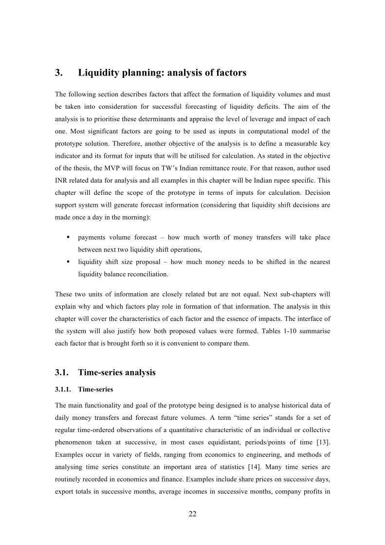
Recent volume is the most important factor. It describes the amount of transfers at recent

calendar days. This is the key determinant that is the basis to the calculation of payments

volume forecast. Input from other factors is applied on top of it to proofread the conclusive

predictable amount of liquidity shift. The format of this key indicator is a single numeric value –

like shown on Figure 5, a deduced sum of all payouts.

Figure 5. Sample of recent volume determinant for liquidity shift planning (Indian rupee)

The blue line (Figure 5) demonstrates daily total sums of transactions where target currency is

specific to particular liquidity buffer. In order to mitigate the risk of miscalculations due to days

with unconventional traffic volumes, it is not only the previous day is taken into account. The

measurable value of this factor is formed based on transfer traffic data of last 2-3 days, it is

visualized with red region. Green region denotes the possible movement of volumes in future.

Table 1. Recent volume factor summary

Factor: Recent volume Key indicator Derivative amount of recently transferred

funds Format Numeric, double precision Magnitude of impact Very high Affects payments volume forecast Yes

Featured in MVP Yes

25

3.2.2. Growth trends

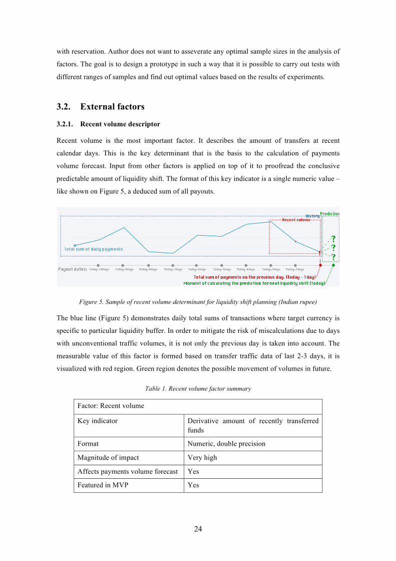
Rapid growth is a characteristic of TransferWise on many different levels – for instance

marketing-driven, invite-program based or plain organic growth. Day after day, TW reaches

more and more people around the world via marketing campaigns. TW has outstanding

performance figures on virality growth, many users recommend the service to their friends and

family. Figure 6, which is based on statistics from Google Trends, displays very vividly how

Internet users’ interest against TransferWise has been growing since the establishment of the

company in 2011 – sixfold a year on the average.

Growing interest against the service brings more new users, the number of transactions ascends

and the overall volume of funds being transferred also grows. Every route has its own growth

rate. It depends on marketing focus or, for example, cultural characteristics. For instance, a TV

advertisement targeting Indian expats in Great Britain can have radical and sharp impact on

“GBP to INR” route growth trend. Also, some nationalities are more inclined to word of mouth

marketing than others.

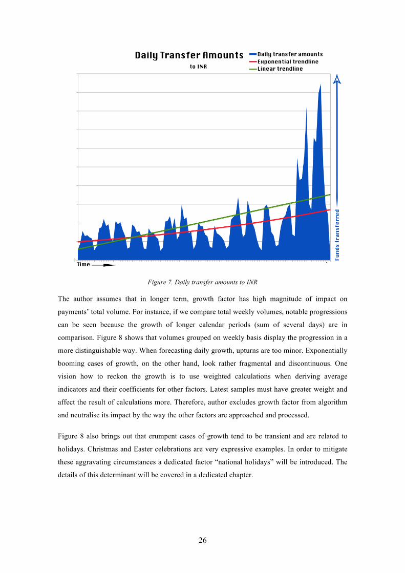
If we inspect the curve of money transfers to Indian rupee on Figure 7, we can see that there is a

specific sinusoidal pattern. Projected trend lines display growth that is easily visible. The

progression is especially remarkable in April 2015 when volumes started to grow exponentially,

increasing threefold in less than 10 days. It was related to very successful INR targeted affiliate

marketing agreement that TW had made.

Figure 6. Google Trends: Interest against term “TransferWise” since establishment of the company

26

Figure 7. Daily transfer amounts to INR

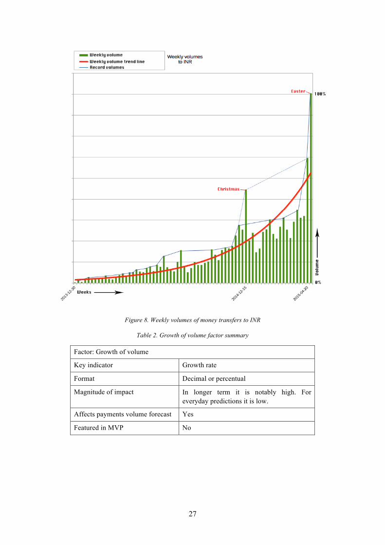
The author assumes that in longer term, growth factor has high magnitude of impact on

payments’ total volume. For instance, if we compare total weekly volumes, notable progressions

can be seen because the growth of longer calendar periods (sum of several days) are in

comparison. Figure 8 shows that volumes grouped on weekly basis display the progression in a

more distinguishable way. When forecasting daily growth, upturns are too minor. Exponentially

booming cases of growth, on the other hand, look rather fragmental and discontinuous. One

vision how to reckon the growth is to use weighted calculations when deriving average

indicators and their coefficients for other factors. Latest samples must have greater weight and

affect the result of calculations more. Therefore, author excludes growth factor from algorithm

and neutralise its impact by the way the other factors are approached and processed.

Figure 8 also brings out that erumpent cases of growth tend to be transient and are related to

holidays. Christmas and Easter celebrations are very expressive examples. In order to mitigate

these aggravating circumstances a dedicated factor “national holidays” will be introduced. The

details of this determinant will be covered in a dedicated chapter.

27

Figure 8. Weekly volumes of money transfers to INR

Table 2. Growth of volume factor summary

Factor: Growth of volume Key indicator Growth rate Format Decimal or percentual Magnitude of impact In longer term it is notably high. For

everyday predictions it is low. Affects payments volume forecast Yes

Featured in MVP No

28

3.2.3. Weekly patterns

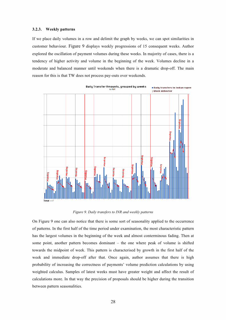
If we place daily volumes in a row and delimit the graph by weeks, we can spot similarities in

customer behaviour. Figure 9 displays weekly progressions of 15 consequent weeks. Author

explored the oscillation of payment volumes during these weeks. In majority of cases, there is a

tendency of higher activity and volume in the beginning of the week. Volumes decline in a

moderate and balanced manner until weekends when there is a dramatic drop-off. The main

reason for this is that TW does not process pay-outs over weekends.

Figure 9. Daily transfers to INR and weekly patterns

On Figure 9 one can also notice that there is some sort of seasonality applied to the occurrence

of patterns. In the first half of the time period under examination, the most characteristic pattern

has the largest volumes in the beginning of the week and almost conterminous fading. Then at

some point, another pattern becomes dominant – the one where peak of volume is shifted

towards the midpoint of week. This pattern is characterised by growth in the first half of the

week and immediate drop-off after that. Once again, author assumes that there is high

probability of increasing the correctness of payments’ volume prediction calculations by using

weighted calculus. Samples of latest weeks must have greater weight and affect the result of

calculations more. In that way the precision of proposals should be higher during the transition

between pattern seasonalities.

29

Table 3. Weekly patterns factor summary

Factor: Weekly patterns

Key indicator Derived average coefficients per day

Format Decimal or percentual

Magnitude of impact Vividly high

Affects payments volume forecast Yes

Featured in MVP Yes

3.2.4. Monthly patterns

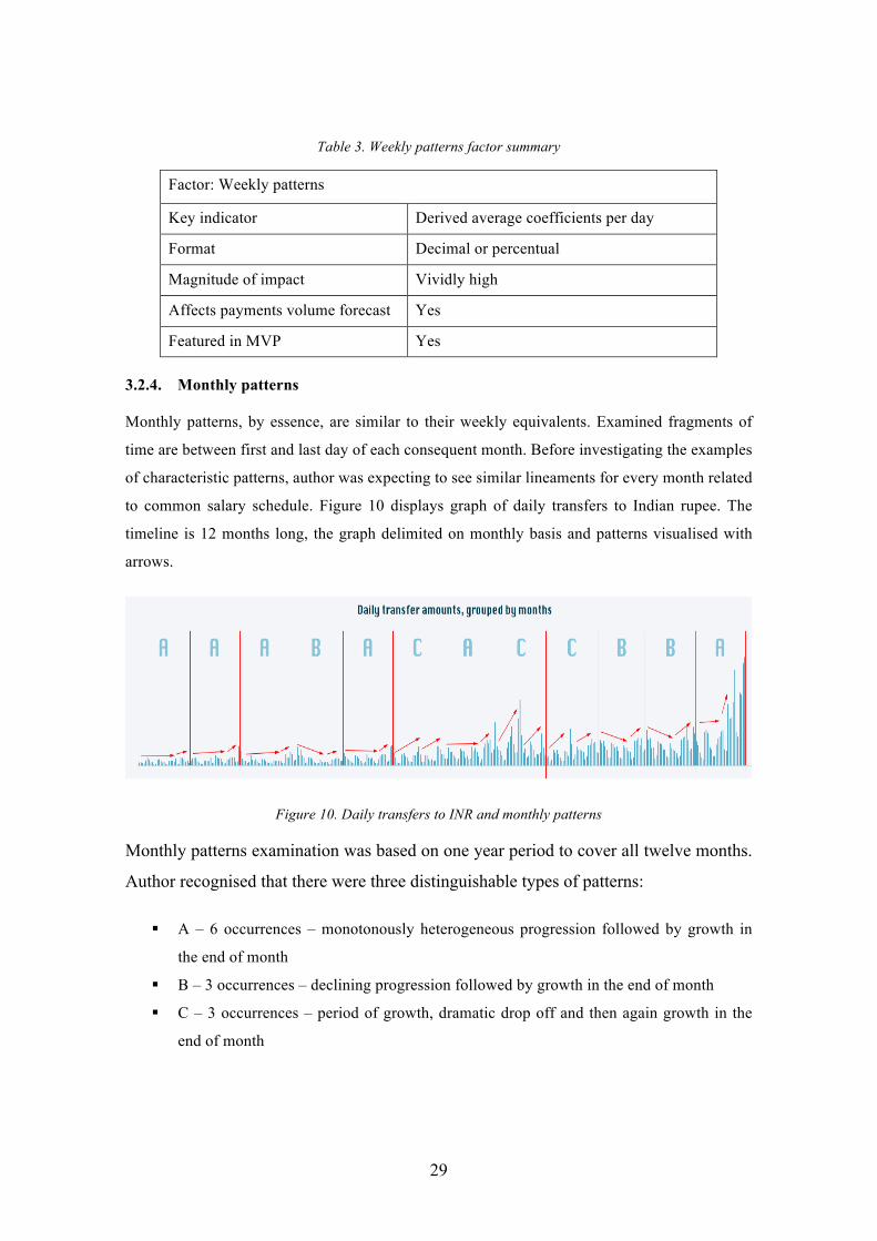
Monthly patterns, by essence, are similar to their weekly equivalents. Examined fragments of

time are between first and last day of each consequent month. Before investigating the examples

of characteristic patterns, author was expecting to see similar lineaments for every month related

to common salary schedule. Figure 10 displays graph of daily transfers to Indian rupee. The

timeline is 12 months long, the graph delimited on monthly basis and patterns visualised with

arrows.

Figure 10. Daily transfers to INR and monthly patterns

Monthly patterns examination was based on one year period to cover all twelve months.

Author recognised that there were three distinguishable types of patterns:

§ A – 6 occurrences – monotonously heterogeneous progression followed by growth in

the end of month

§ B – 3 occurrences – declining progression followed by growth in the end of month

§ C – 3 occurrences – period of growth, dramatic drop off and then again growth in the

end of month

30

One characteristic shared by every pattern is the increase of volumes in the end of

calendar month. Main reason for that is that people get paid often at end or beginning of

month and also the deadline of bills to pay is normally at month end.

Table 4. Monthly patterns factor summary

Factor: Monthly patterns

Key indicator Derived coefficients per day

Format Decimal or percentual

Magnitude of impact Medium

Affects payments volume forecast Yes

Featured in MVP Yes

3.2.5. Exchange rate movements

Experience of people who deal with liquidity management shows that some particular routes are

very sensitive to exchange rate movements. Some groups of customers become strongly active

when the rate of their target currency is showing growth and calm down if the exchange rate

movement is adverse. Such phenomenon is common for different currency routes and Indian

customers are also very good example. Indians, being the world's second most populous nation,

have large scale diaspora widespread most notably in Southeast Asia, United Kingdom, North

America, Australia, South Africa and Southern Europe. Diaspora population estimates vary

from a 12 million to 20 million [16]. When the exchange rate gets in favourable state, Indian

expats around the whole world use the remittance service notably a lot more actively. Figure 11

shows an example of real USD/INR exchange rate progression and illustrates the accompanying

intensity of transfer activity to Indian rupee.

Figure 11. Example of USD/INR exchange rate movement

31

Green coloured regions of the exchange rate curve visualise a positive direction of rate

movement, red ones display the deprecation. The background of graph’s grid is distinguished

into green, red and yellow areas. Green areas mark down time periods when progression of

exchange rate has an identifiable positive impact on frequency of transfers to Indian rupee. Red

areas denote periods when corresponding activity diminishes. The density of color accentuates

the intensity of these tendencies. Longer ups and downs have greater impact. Yellow areas mark

periods when situation normalises and exchange rate factor has no perceiveable impact on

frequency/volume of transfers.

Table 5. Exchange rate movement factor summary

Factor: Exchange rate movement

Key indicator Growth rate change

Format Decimal or percentual

Magnitude of impact Depending on particular routes and size of fluctuations can be notably high

Affects payments volume forecast Yes

Featured in MVP No

3.2.6. Frequency of extra large payment orders

High feedback ratings, fundraising from well-known high-profile venture capitalists, stable

service and continuous product improvement give rise to big customers’ trust against the

service. Customers have trusted already $4.5 billion [5] worth of money transfers. While

majority of payments, in terms of size, are roughly near average, strikingly large payments

occur quite often as well. Such big scale single transfers can be tens or even hundreds times

bigger than the average. It happens that customers transfer funds worth of several million

pounds in single payment [5].

Needless to say, extraordinarily big transfers might be a serious impediment for forecasting

algorithm. Author analysed the history of transfers to Indian rupee and collected statistics about

occurrences of transfers exceeding the average size by several times.

Figure 12 visualises the frequency of extra large payments. The graph shows that defined extra

large transfers take place roughly at half of the days. Figure 12 also brings under notice that the

growth of overall volumes in 2015 also uplifted the frequency of big payments. Author assumes

that knowledge regarding the density of these payments makes it possible to forecast

statistically when to expect them in future. The priority of this factor is not very high because

normally pay-outs of eminently big payments are just adjourned over one extra day. However, it

32

would be great if liquidity planning decision support system could help to cover at least some of

them and speed up their payout process.

Figure 12. Frequency of extra large transfers to Indian rupee

Table 6. Frequency of large payments factor summary

Factor: Frequency of large payments

Key indicator Relative frequency ratio

Format Decimal

Magnitude of impact In case of occurance of large payments: ~5% on the average, low

Affects payments volume forecast Yes

Featured in MVP No  

3.2.7. National Holidays

Figure 8 is focused on weekly transaction volumes but it also vividly brings forth that transfer

activity is booming during holiday periods. Once again, India is a great example. Being a

culturally diverse and fervent society, this nation celebrates various holidays and festivals that,

from remittance point of view, have instant impact on volume of transfers. In addition to

national holidays, there are Hindu, Islamic, Christian, Sikh, Buddhist, Jain celebrations. Also in

respect of Banks, most notable holidays are restricted to 15 days in a year in terms of the

instructions issued by the Department of Economic Affairs [17]. Bank holidays also affect

transfer activity because there are customers who take these dates into account and consider

sending money in advance to get their funds transferred surely at desirable time.

33

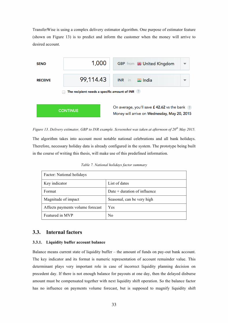
TransferWise is using a complex delivery estimator algorithm. One purpose of estimator feature

(shown on Figure 13) is to predict and inform the customer when the money will arrive to

desired account.

Figure 13. Delivery estimator, GBP to INR example. Screenshot was taken at afternoon of 20th May 2015.

The algorithm takes into account most notable national celebrations and all bank holidays.

Therefore, necessary holiday data is already configured in the system. The prototype being built

in the course of writing this thesis, will make use of this predefined information.

Table 7. National holidays factor summary

Factor: National holidays

Key indicator List of dates

Format Date + duration of influence

Magnitude of impact Seasonal, can be very high

Affects payments volume forecast Yes  Featured in MVP No

3.3. Internal factors

3.3.1. Liquidity buffer account balance

Balance means current state of liquidity buffer – the amount of funds on pay-out bank account.

The key indicator and its format is numeric representation of account remainder value. This

determinant plays very important role in case of incorrect liquidity planning decision on

precedent day. If there is not enough balance for payouts at one day, then the delayed disburse

amount must be compensated together with next liquidity shift operation. So the balance factor

has no influence on payments volume forecast, but is supposed to magnify liquidity shift

34

proposal size in case algorithm detects that liquidity buffer might run out of funds on present

day.

Table 8. Buffer balance factor summary

Factor: Buffer balance Key indicator Account balance in local currency

Format Numeric, double precision

Magnitude of impact Very high in specific cases

Affects payments volume forecast No

Featured in MVP Yes

3.3.2. Suspended transfers

Suspended transfer is a state of TransferWise payment when customer’s money is received but

payment is temporarily put on hold and does not go to conversion. This is the moment when

customer finally knows exactly how much money:

1. will the recipient get in case of fixed source transfers,

2. will be refunded as excess refund in case of fixed target transfers.

For P2P (current two-way) routes, matching term is self-explanatory. Payment gets matched

with customer transfers from opposite routes. Like stated before in Chapter 2.6, at the moment

of writing this thesis TransferWise supports payouts in INR but does not yet allow users to

perform pay-ins with INR. Therefore in the INR corner-case context, matching is a step before

pay-out when the conversion rate gets locked.

Payments can get suspended automatically or manually on various reasons. Mainly when extra

customer verification activities are needed. Customer verification is tricky case because further

customers involvement is needed. Usually customers are motivated to cooperate as soon as

possible because they understand that it will quicken the pay-out process. In reality, it is not

possible to predict when exactly each customer will perform necessary verification steps.

Customer might not have a possibility to submit requested documents quickly or can be just

unavailable. To sum up, it is unknown when and which suspended payments will go into

matching.

After matching, money gets transferred to recipient account within few hours. TransferWise

wants to execute all payments as soon as possible. Business wants to send out the money as

soon as payment is matched. Taking that into consideration, successful liquidity planning

requires not only forecasting of instantly successful payments but also prediction of matching

35

dates of currently suspended transfers. Author assumes that, based on statistical data and

average durations, it is possible to propose an evaluative expected matching time individually

for every suspended transfer. Taking advantage of this data can increase the accurateness of

decision support system prototype.

Table 9. Suspended transfers factor summary

Factor: Suspended transfers

Key indicator Relative frequency ratio

Format Decimal

Magnitude of impact In case of occurrence of large payments: ~5% on the average

Affects payments volume forecast No

Featured in MVP No

3.3.3. Liquidity in transit

Liquidity in transit means funds that were sent with the latest reconciliation and have not yet

reached company’s pay-out buffer account. The key indicator and its format is numeric value of

money in transit. The impact of this factor is very similar to the account balance one. This

determinant is notable in case of incorrect liquidity planning decision on precedent day. Sending

too few funds for pay-outs will cause currency deficit on the next day. Pay-outs will be

postponed. The delayed disburse amount must be then compensated together with next balance

shift operation. So just like the balance factor, funds in transit determinant has no influence on

payments volume forecast. But it is supposed to magnify liquidity shift proposal size in case

algorithm detects that pending liquidity transfer is not big enough to fulfill the expected pay-out

needs. In reality, this factor is more likely a theoretical one, at least in INR case. Normally there

is no unfinished liquidity transfers when new reconciliation planning decisions are being made.

It can theoretically happen if there is some unexpected trouble with liquidity shift transfer which

is a rare corner case. For that reason, author leaves this determinant out of scope and will focus

more on other factors.

Table 10. Liquidity in transit factor summary

Factor: Liquidity in transit

Key indicator Volume of funds in transit

Format Numeric, double

Affects payments volume forecast No

Featured in MVP No

36

4. Liquidity planner: Computational model

The purpose of this chapter is to describe how indications from selected problem factors

(analysed in 3) are used to calculate the forecast.

4.1. Data processing methods

This chapter will introduce and explain some data series processing methods that are common

for calculation of different factors formulated and described in Chapter 3.

4.1.1. Data transformation

The computational model in MVP solution is using several data transformation operations

known from data mining and other data processing fields. The aim of this chapter is to expound

the meaning of terms that are used in Chapter 4.2. In data transformation, the time series data or

their sub-parts are transformed or consolidated into forms appropriate for further processing

steps. Data transformation types featured in this computational model are following:

§ Smoothing is used to remove noise from the data.

§ Aggregation – summary or aggregation operations are applied to the data. For example,

the daily transfer volumes data may be aggregated so as to compute monhtly and annual

total amounts.

§ Generalisation – low level or ‘primitive’ (raw) data are replaced by higher-level

concepts through the use of concept hierarchies [18]. In the context of this thesis, the

example of generalisation is when sub-parts of time series are aggregated into separate

weeks or months and handled as distinct entities.

§ Normalisation – the attribute data are scaled so as to fall within a specified range, such

as 0.0 to 1.0, or 0 to 100.

4.1.2. Moving average

A moving average is a method for smoothing time series by averaging (with or without weights)

a fixed number of consecutive terms. The averaging “moves” over time, in that each data point

of the series is sequentially included in the averaging, while the oldest data point in the span of

the average is removed. In general, the longer the span of the average is, the smoother is the

resulting series [13]. Moving averages are used to smooth fluctuations in time series or to

identify time series components, such as the trend, the cycle, the seasonal, etc [13].

37

A moving average replaces each value of a time series by an average of p preceding values, the

given value and f following values of a series. If p = f the moving average is said to be centered.

The moving average is said to be symmetric if it is centered, and if for each k=1,2,..., p = f, the

weight of the k-th preceding value is equal to the weight of the k-th following one [13].

There are several variations of moving average computation techniques used for smoothing

time-series. Some examples are single moving average (SMA), moving average with trends,

weighted moving average or double moving average (DMA) [13] [19]. Author will use non-

centered SMA and non-centered DMA techniques.

Single moving average is the most basic method, consequent samples from data series are used

as input together with period p that determines which data point of the series must be the oldest

in span of the average. When a moving average is taken of a series of data that already

represents the result of a moving average, it is referred to as a double moving average. It results

in additional smoothing or the removal of more randomness than an equal/length single moving

average [20]. So, as the name implies, the double moving average technique involves taking the

average of averages.

4.1.3. Weighted arithmetic mean

The weighted arithmetic mean is similar to an ordinary arithmetic mean which is the most

common type of average. In the computation of arithmetic mean, equal importance is given to

all the items of the series. However, there are cases where all the items are not of equal

importance, and importance itself is relative by nature. In other words, some items of a series

are more important as compared to the other items in the same series. In such cases, it becomes

important to assign different weights to different items. The weighted mean can be used to

calculate an average that takes into account the importance of each value with respect to the

overall total [21].

The formula for calculating weighted mean is given by Formula 1, where x is the values of the

variable and w the weights attached to values of the variable [22].

𝑥 = !×!!

(1)

In the context of this thesis, author assumes that in many cases older time series samples have

less importance and therefore must have less weight. If all the weights are equal, then the

weighted mean is the same as the arithmetic mean. The notion of weighted mean plays a role in

descriptive statistics and also occurs in a more general form in several other areas of

mathematics.

38

4.2. Calculation of factors

4.2.1. Recent volume

Recent volume (R) is simple calculation. The inputs of the algorithm are:

§ Value T – Time series (list of samples),

§ Value Pr – Pointer to last day’s sample,

§ Value Nr – Value Number of preceding samples to use,

§ Value WMr – Whether to apply weighted mean.

Algorithm takes the defined sample Pr from time series T, normally the preceding calendar day

of forecast calculation. Based on input Nr value, it extracts Nr-1 more preceding samples. Then

it calculates the average value of selected samples. Based on input parameter Pr, the algorithm

decides whether to apply the weighted calculation approach. If weighted calculation is used,

then each next sample has 1/Nr smaller weight and therefore smaller impact on the calculation

result.

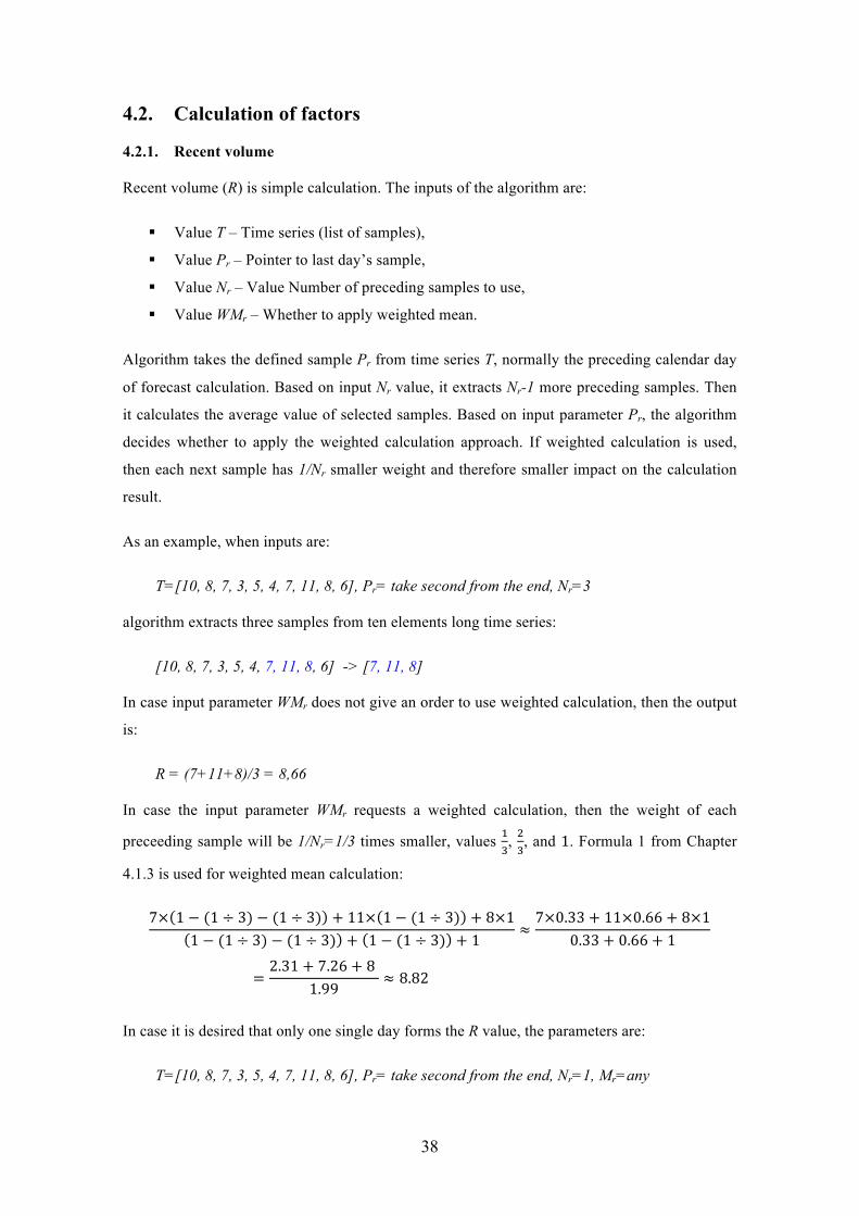
As an example, when inputs are:

T=[10, 8, 7, 3, 5, 4, 7, 11, 8, 6], Pr= take second from the end, Nr=3

algorithm extracts three samples from ten elements long time series:

[10, 8, 7, 3, 5, 4, 7, 11, 8, 6] -> [7, 11, 8]

In case input parameter WMr does not give an order to use weighted calculation, then the output

is:

R = (7+11+8)/3 = 8,66

In case the input parameter WMr requests a weighted calculation, then the weight of each

preceeding sample will be 1/Nr=1/3 times smaller, values !!, !!, and 1. Formula 1 from Chapter

4.1.3 is used for weighted mean calculation:

7× 1 − (1 ÷ 3) − (1 ÷ 3) + 11× 1 − (1 ÷ 3) + 8×11 − (1 ÷ 3) − (1 ÷ 3) + 1 − (1 ÷ 3) + 1

≈7×0.33 + 11×0.66 + 8×1

0.33 + 0.66 + 1

=2.31 + 7.26 + 8  

1.99≈ 8.82

In case it is desired that only one single day forms the R value, the parameters are:

T=[10, 8, 7, 3, 5, 4, 7, 11, 8, 6], Pr= take second from the end, Nr=1, Mr=any

39

Nr=1 means that the output of the algorithm is based on only one element of the series.

[10, 8, 7, 3, 5, 4, 7, 11, 8, 6] -> [8]

Input parameters Nr and WMr allow to carry out tests in various different ways and find out in

practice, which recent volume derivation technique is the most suitable.

4.2.2. Weekly patterns

The inputs for weekly pattern (W) calculation are:

§ Value T – Time series (list of samples),

§ Value Pw – Pointer to last day’s sample,

§ Value Nw – Number of weeks to take into account,

§ Value WMw – Whether to apply weighted mean.

The weekly patterns algorithm takes the defined sample Pw from time series T, normally the

preceding calendar day of forecast calculation. Based on input value Nw, it extracts Nw preceding

weeks, or simply Nw*7 preceding samples (time series days). Extraction:

[T] => [1st week], [2nd week],…,[Nwth week] where each [week] contains 7 days’ data.

Algorithm compares the daily transfer volumes of each day in these weeks. Each sample in the

week’s data series is divided by the week’s highest value. As a result, generalised weekly

datasets do not represent absolute volume numbers, because the data is normalised and

presented on a scale from 0.0 to 1.0. The result of normalisation reflects daily coefficients

relative to each other. Array of volumes gets transformed into map of coefficients. As a simple

example, if daily values of Nwth week are [10, 8, 6, 5, 9, 2, 3] then the normalised representation

will be [1, 0.8, 0.6, 0.5, 0.9, 0.2, 0.3] where all values are simply scaled down ten times because

the greatest value in the original data range is 10. If the first element represents Monday, then

coefficients in this example show that the volume of Saturday was five times smaller than on

Monday (1/0.2=5).

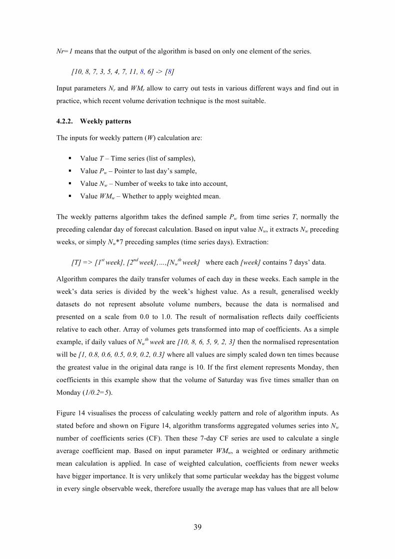
Figure 14 visualises the process of calculating weekly pattern and role of algorithm inputs. As

stated before and shown on Figure 14, algorithm transforms aggregated volumes series into Nw

number of coefficients series (CF). Then these 7-day CF series are used to calculate a single

average coefficient map. Based on input parameter WMw, a weighted or ordinary arithmetic

mean calculation is applied. In case of weighted calculation, coefficients from newer weeks

have bigger importance. It is very unlikely that some particular weekday has the biggest volume

in every single observable week, therefore usually the average map has values that are all below

40

1. After that, all coefficients are scaled up, this time in a way that the weekday of Pw becomes

equal to 1.0.

Figure 14. Weekly pattern calculation steps

An example of calculated average week coefficients (following example is based on real

operational output of already implemented computation in prototype. Values and precision are

reduced):

§ Monday: 0.68309

§ Tuesday: 0.70659

§ Wednesday: 0.72790

§ Thursday: 0.72336

§ Friday: 0.56492

§ Saturday: 0.25342

§ Sunday: 0.23236

For instance, if the weekday of Pw is Tuesday and Tuesday’s value in average coefficient map

is PwV, then we apply a simple formula (Formula 2) to all samples:

𝑥 = 𝑥× !.!!"#

= !!"#

(2)

where x is new value for some day and x is the old one. For Monday it would be:

41

𝑥 = 0.68309×1.0

0.70659=0.683090.72336

≈ 0.96673  

If we applied to all weekdays, then the result W is:

§ Monday: 0.96673

§ Tuesday: 1.0

§ Wednesday: 1.03016

§ Thursday: 1.02373

§ Friday: 0.79950

§ Saturday: 0.35865

§ Sunday: 0.32885

Based on this example, the pattern states that it is likely that volumes on Fridays are 20%

smaller than on Tuesdays (~0.8 vs. 1). Again, in a similar way to recent volume calculation

algorithm, input parameters Nw and WMw make it possible to carry out tests in various different

ways and find out in practice which settings work in a best way for calculating weekly patterns.

4.2.3. Monthly patterns

Monthly pattern (M) algorithm is similar to weekly one but the proposed calculation is more

complex. When compared to weekly patterns, monthly seasonality is more difficult because the

timespan is longer and the length of months is varying. The inputs of the algorithm are:

§ Value T – Time series (list of samples)

§ Value Pm – Pointer to day prior to forecast

§ Value Mn – Number of preceeding last full months to analyse

§ Value MA – Whether to apply moving average smoothing

o MAsd – Whether to use single or double moving average filter

o MAr – Smoothing radius

The proposed algorithm performs calculations only on complete finished months. It is done like

that because the goal is to generalise trends of past months into a single characteristic pattern.

Incomplete month does not implicitly describe the progression of monthly volumes. Again,

when comparing to weekly patterns, approach used there was extracting weeks starting from

day Pw (in monthly pattern approach, the analogous variable is Pm) in time series T. In monthly

pattern calculation, it can only happen if Pm is the last day of current month. So if Pm is

somewhere in the middle of the month, then this month’s data samples are skipped and not used

for calculations. Figure 15 visualises that data aggregation for extracting months is shifted to the

left in time series T span. Similarly to week pattern calculation, values in every extracted month

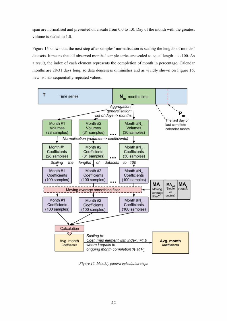
42

span are normalised and presented on a scale from 0.0 to 1.0. Day of the month with the greatest

volume is scaled to 1.0.

Figure 15 shows that the next step after samples’ normalisation is scaling the lengths of months’

datasets. It means that all observed months’ sample series are scaled to equal length – to 100. As

a result, the index of each element represents the completion of month in percentage. Calendar

months are 28-31 days long, so data denseness diminishes and as vividly shown on Figure 16,

new list has sequentially repeated values.

Figure 15. Monthly pattern calculation steps

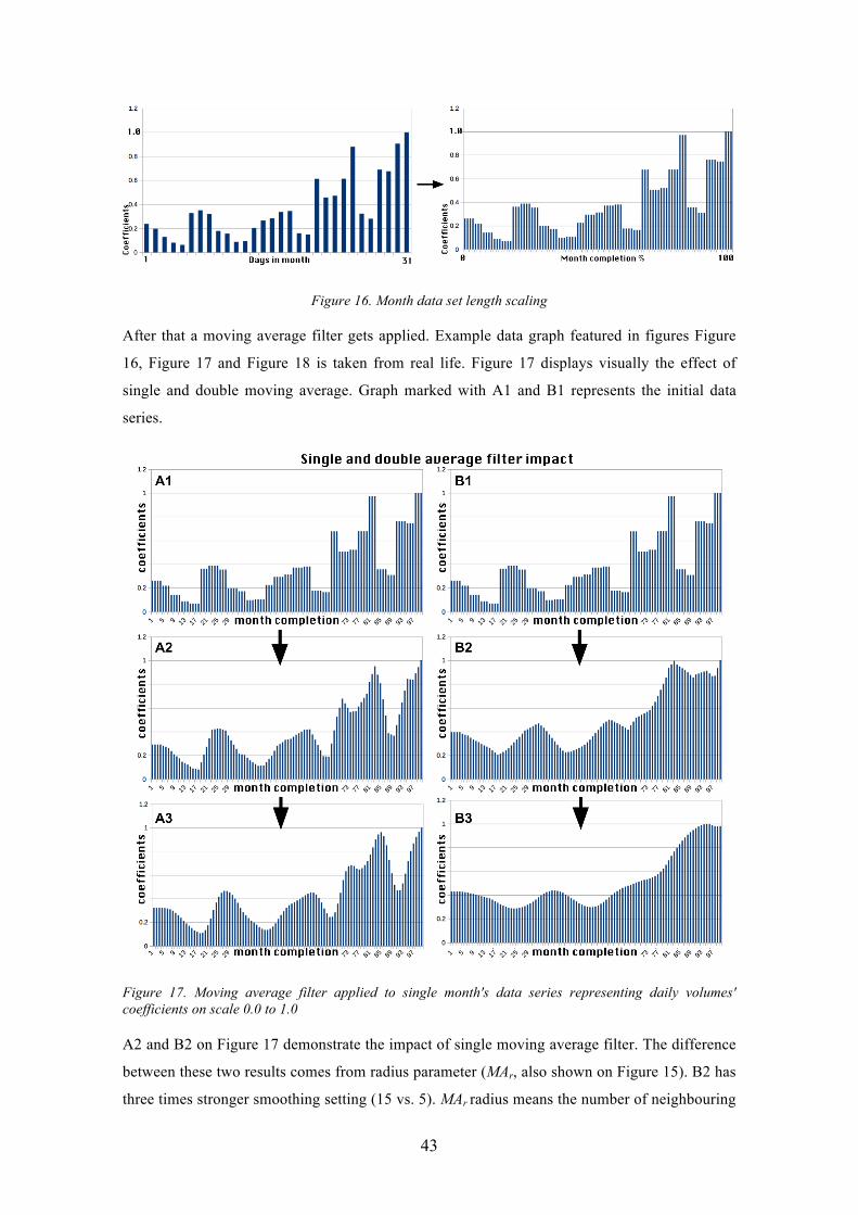
43

Figure 16. Month data set length scaling

After that a moving average filter gets applied. Example data graph featured in figures Figure

16, Figure 17 and Figure 18 is taken from real life. Figure 17 displays visually the effect of

single and double moving average. Graph marked with A1 and B1 represents the initial data

series.

Figure 17. Moving average filter applied to single month's data series representing daily volumes' coefficients on scale 0.0 to 1.0

A2 and B2 on Figure 17 demonstrate the impact of single moving average filter. The difference

between these two results comes from radius parameter (MAr, also shown on Figure 15). B2 has

three times stronger smoothing setting (15 vs. 5). MAr radius means the number of neighbouring

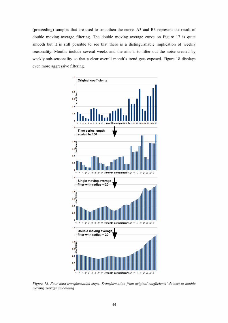
44

(preceeding) samples that are used to smoothen the curve. A3 and B3 represent the result of

double moving average filtering. The double moving average curve on Figure 17 is quite

smooth but it is still possible to see that there is a distinguishable implication of weekly

seasonality. Months include several weeks and the aim is to filter out the noise created by

weekly sub-seasonality so that a clear overall month’s trend gets exposed. Figure 18 displays

even more aggressive filtering.

Figure 18. Four data transformation steps. Transformation from original coefficients’ dataset to double moving average smoothing

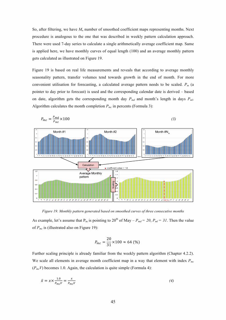
45

So, after filtering, we have Mn number of smoothed coefficient maps representing months. Next

procedure is analogous to the one that was described in weekly pattern calculation approach.

There were used 7-day series to calculate a single arithmetically average coefficient map. Same

is applied here, we have monthly curves of equal length (100) and an average monthly pattern

gets calculated as illustrated on Figure 19.

Figure 19 is based on real life measurements and reveals that according to average monthly

seasonality pattern, transfer volumes tend towards growth in the end of month. For more

convenient utilisation for forecasting, a calculated average pattern needs to be scaled. Pm (a

pointer to day prior to forecast) is used and the corresponding calendar date is derived – based

on date, algorithm gets the corresponding month day Pmd and month’s length in days Pml.

Algorithm calculates the month completion Pmc in percents (Formula 3):

𝑃!" =!!"!!"

×100 (3)

Figure 19. Monthly pattern generated based on smoothed curves of three consecutive months

As example, let’s assume that Pm is pointing to 20th of May – Pmd = 20, Pml = 31. Then the value

of Pmc is (illustrated also on Figure 19):

𝑃!" =2031×100 ≈ 64  (%)

Further scaling principle is already familiar from the weekly pattern algorithm (Chapter 4.2.2).

We scale all elements in average month coefficient map in a way that element with index Pmc

(PmcV) becomes 1.0. Again, the calculation is quite simple (Formula 4):

𝑥 = 𝑥× !.!!!"!

= !!!"!

(4)

46

where x is new value for some day and x is the old one. Figure 19 demonstrates how coefficient

with index 64 becomes valued 1.0 and all other coefficients change proportionally. A

completely scaled coefficient map is average monthly pattern M that is used later in forecast.

To forecast 21st May, we calculate the completion of the month 21/31*100=70 (%) and

compare elements 64 and 70 in coefficient map. Depending on month, we may always skip 1-7

elements but they are not useless, because they were used to smoothen the values that are

utilised for forecasting.

Example of scaled coefficient graph on Figure 19 shows that coefficient with index 70 has

slightly smaller value than the one with index 64. It means that according to the calculated

average monthly trend, volumes are likely to decline but the difference is insignificant.

4.2.4. Liquidity buffer account balance

There are two important determinants related to account balance value:

§ A – Account balance state,

§ D – Deficit.

Determinant A was covered in Chapter 3.3.1. Account balance state describes the amount of

funds on pay-out bank account. The proposed algorithm takes into account the balance state, if

there is enough funds to perform the payouts on the following days, then proposal system must

not demand for liquidity shift. This determinant plays also very important role in case of

incorrect liquidity planning decision on precedent day. If there is not enough balance for

payouts at one day, then the delayed disburse amount must be compensated together with the

next liquidity shift operation. If such undesirable situation occurs, then there will be a list of

pending overdue payouts. Deficit D stands for a total volume of overdue payments.

4.2.5. Forecast and reconciliation proposal

Like stated in Chapter 3 the objective of prototype is to calculate two things:

§ F – payments volume forecast – how much worth of money transfers will take place

between next two liquidity shift operations,

§ P – liquidity shift size proposal – how much money needs to be shifted in the nearest

liquidity balance reconciliation.

This chapter sums up the computational model chapter and connects together different steps of

computations mentioned above. Input parameters for volume forecast and liquidity shift

proposal are:

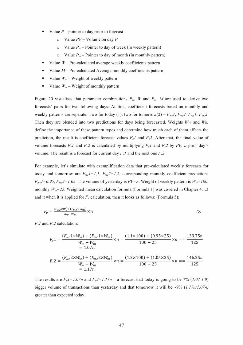
47

§ Value P – pointer to day prior to forecast

o Value PV – Volume on day P

o Value Pw – Pointer to day of week (in weekly pattern)

o Value Pm – Pointer to day of month (in monthly pattern)

§ Value W – Pre-calculated average weekly coefficients pattern

§ Value M – Pre-calculated Average monthly coefficients pattern

§ Value Ww – Weight of weekly pattern

§ Value Wm – Weight of monthly pattern

Figure 20 visualises that parameter combinations Pw, W and Pm, M are used to derive two

forecasts’ pairs for two following days. At first, coefficient forecasts based on monthly and

weekly patterns are separate. Two for today (1), two for tomorrow(2) – Fwc1, Fwc2, Fmc1, Fmc2.

Then they are blended into two predictions for days being forecasted. Weights Ww and Wm

define the importance of these pattern types and determine how much each of them affects the

prediction, the result is coefficient forecast values Fc1 and Fc2. After that, the final value of

volume forecasts Fv1 and Fv2 is calculated by multiplying Fc1 and Fc2 by PV, a prior day’s

volume. The result is a forecast for current day Fv1 and the next one Fv2.

For example, let’s simulate with exemplification data that pre-calculated weekly forecasts for

today and tomorrow are Fwc1=1,1, Fwc2=1,2, corresponding monthly coefficient predictions

Fmc1=0.95, Fmc2=1.05. The volume of yesterday is PV=n. Weight of weekly pattern is Ww=100,

monthly Wm=25. Weighted mean calculation formula (Formula 1) was covered in Chapter 4.1.3

and it when it is applied for Fv calculation, then it looks as follows: (Formula 5):

𝐹! =!!"×! ! !!"×!!

!!!!!×𝑛 (5)

Fv1 and Fv2 calculation:

𝐹!1 =𝐹!"1×𝑊! + 𝐹!"1×𝑊!

𝑊! +𝑊!×𝑛 =

1.1×100 + 0.95×25100 + 25

×𝑛 ==133.75𝑛125

= 1.07𝑛

𝐹!2 =𝐹!"2×𝑊! + 𝐹!"2×𝑊!

𝑊! +𝑊!×𝑛 =

1.2×100 + 1.05×25100 + 25

×𝑛 ==146.25𝑛125

= 1.17𝑛

The results are Fv1=1.07n and Fv2=1.17n – a forecast that today is going to be 7% (1.07-1.0)

bigger volume of transactions than yesterday and that tomorrow it will be ~9% (1,17n/1.07n)

greater than expected today.

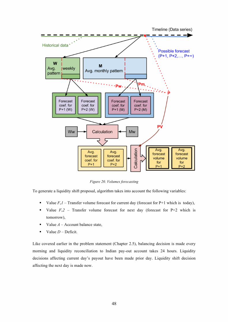
48

Figure 20. Volumes forecasting

To generate a liquidity shift proposal, algorithm takes into account the following variables:

§ Value Fv1 – Transfer volume forecast for current day (forecast for P+1 which is today),

§ Value Fv2 – Transfer volume forecast for next day (forecast for P+2 which is

tomorrow),

§ Value A – Account balance state,

§ Value D – Deficit.

Like covered earlier in the problem statement (Chapter 2.5), balancing decision is made every

morning and liquidity reconciliation to Indian pay-out account takes 24 hours. Liquidity

decisions affecting current day’s payout have been made prior day. Liquidity shift decision

affecting the next day is made now.

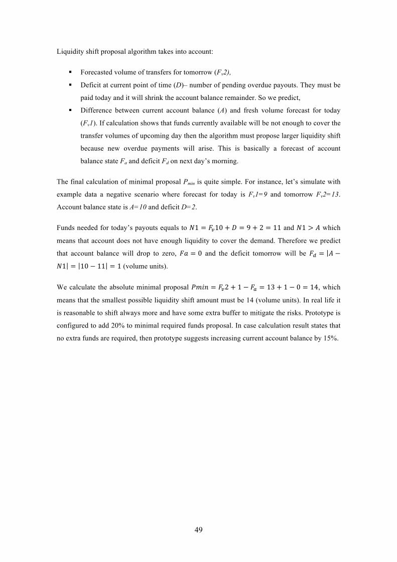
49

Liquidity shift proposal algorithm takes into account:

§ Forecasted volume of transfers for tomorrow (Fv2),

§ Deficit at current point of time (D)– number of pending overdue payouts. They must be

paid today and it will shrink the account balance remainder. So we predict,

§ Difference between current account balance (A) and fresh volume forecast for today

(Fv1). If calculation shows that funds currently available will be not enough to cover the

transfer volumes of upcoming day then the algorithm must propose larger liquidity shift

because new overdue payments will arise. This is basically a forecast of account

balance state Fa and deficit Fd on next day’s morning.

The final calculation of minimal proposal Pmin is quite simple. For instance, let’s simulate with

example data a negative scenario where forecast for today is Fv1=9 and tomorrow Fv2=13.

Account balance state is A=10 and deficit D=2.

Funds needed for today’s payouts equals to 𝑁1 = 𝐹!10 + 𝐷 = 9 + 2 = 11 and 𝑁1 > 𝐴 which

means that account does not have enough liquidity to cover the demand. Therefore we predict

that account balance will drop to zero, 𝐹𝑎 = 0 and the deficit tomorrow will be 𝐹! = 𝐴 −

𝑁1 = 10 − 11 = 1 (volume units).

We calculate the absolute minimal proposal 𝑃𝑚𝑖𝑛 = 𝐹!2 + 1 − 𝐹! = 13 + 1 − 0 = 14, which

means that the smallest possible liquidity shift amount must be 14 (volume units). In real life it

is reasonable to shift always more and have some extra buffer to mitigate the risks. Prototype is

configured to add 20% to minimal required funds proposal. In case calculation result states that

no extra funds are required, then prototype suggests increasing current account balance by 15%.

50

5. Liquidity planner MVP

5.1. Implementation

The prototype is implemented in Groovy language and is based on Grails application

framework. Author decided to choose these facilities because large part of payment processing

codebase in TW is written in Groovy and Grails. Potential future integration with real system

will be the easiest if used technologies and tools match.

5.1.1. Groovy and Grails

Groovy is an expressive object oriented scripting language, which comes with an array of

features conducive for rapid software development and hence high developer productivity. The

language has Java-like syntax and provides seamless access to Java API. Its compiler generates

Java Virtual Machine (JVM) compatible byte code [23]. The similarities with Java language

make it easier for the developers to acquire functional knowledge in Groovy. However, the

objective is not to replace system-programing languages like Java but to complement them and

empower the developer in producing less yet robust code.

Groovy is weakly typed language i.e. the type of object is determined at runtime and is not

dependent on the variable holding the object reference. This allows different usage of the same

variable in different situations, and hence introduces flexibility.

The power of this language is evident from the higher level of abstraction it offers through

native support for data structures like Maps and Lists as well as availability of closures and

builders. Processing of aforementioned data structures and even database records can be

handled by closures. The possibility of referencing closures by variables, passing them as

parameter to method, declaring them as instance field of classes, and parameterisation for

generalisation makes them a powerful feature.

Grails is a next generation full stack application framework, which tightly integrates with Java

and leverages the dynamic language Groovy for its simplicity, syntactic expressiveness, and

flexibility [24]. Additionally it facilitates blending of Java and Groovy through mixing of static

and dynamic code.

Grails builds on the underlying powerful Java features and exposes the embraced mature

frameworks and APIs through simplified interfaces. The usage thereof does not deviate from

well-documented configuration, or restrain development capabilities. The framework essentially

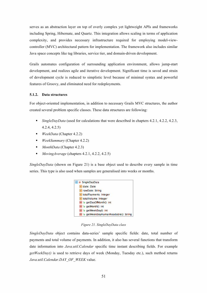
51

serves as an abstraction layer on top of overly complex yet lightweight APIs and frameworks

including Spring, Hibernate, and Quartz. This integration allows scaling in terms of application

complexity, and provides necessary infrastructure required for employing model-view-

controller (MVC) architectural pattern for implementation. The framework also includes similar

Java space concepts like tag libraries, service tier, and domain-driven development.

Grails automates configuration of surrounding application environment, allows jump-start

development, and realizes agile and iterative development. Significant time is saved and strain

of development cycle is reduced to simplistic level because of minimal syntax and powerful

features of Groovy, and eliminated need for redeployments.

5.1.2. Data structures

For object-oriented implementation, in addition to necessary Grails MVC structures, the author

created several problem specific classes. These data structures are following:

§ SingleDayData (used for calculations that were described in chapters 4.2.1, 4.2.2, 4.2.3,

4.2.4, 4.2.5)

§ WeekData (Chapter 4.2.2)

§ WeekSummary (Chapter 4.2.2)

§ MonthData (Chapter 4.2.3)

§ MovingAverage (chapters 4.2.1, 4.2.2, 4.2.5)

SingleDayData (shown on Figure 21) is a base object used to describe every sample in time

series. This type is also used when samples are generalised into weeks or months.

Figure 21. SingleDayData class

SingleDayData object contains data-series’ sample specific fields: date, total number of

payments and total volume of payments. In addition, it also has several functions that transform

date information into Java.util.Calendar specific time instant describing fields. For example

getWeekDay() is used to retrieve days of week (Monday, Tuesday etc.), such method returns

Java.util.Calendar.DAY_OF_WEEK value.

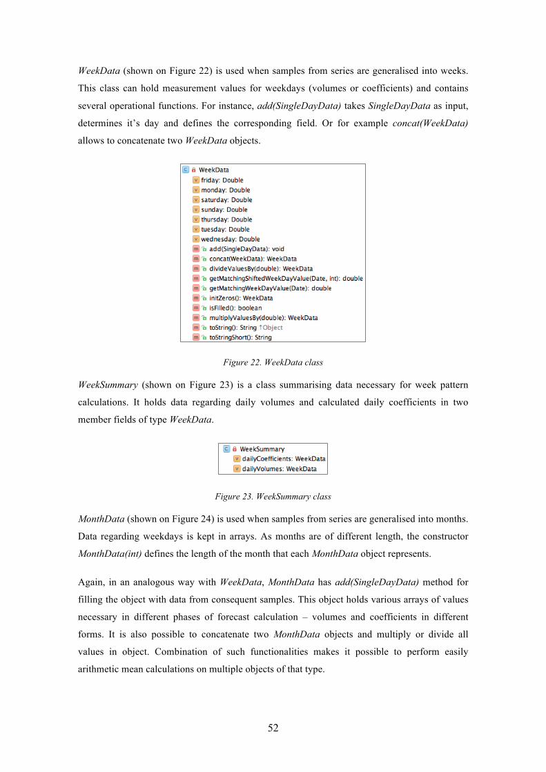
52

WeekData (shown on Figure 22) is used when samples from series are generalised into weeks.

This class can hold measurement values for weekdays (volumes or coefficients) and contains

several operational functions. For instance, add(SingleDayData) takes SingleDayData as input,

determines it’s day and defines the corresponding field. Or for example concat(WeekData)

allows to concatenate two WeekData objects.

Figure 22. WeekData class

WeekSummary (shown on Figure 23) is a class summarising data necessary for week pattern

calculations. It holds data regarding daily volumes and calculated daily coefficients in two

member fields of type WeekData.

Figure 23. WeekSummary class

MonthData (shown on Figure 24) is used when samples from series are generalised into months.

Data regarding weekdays is kept in arrays. As months are of different length, the constructor

MonthData(int) defines the length of the month that each MonthData object represents.

Again, in an analogous way with WeekData, MonthData has add(SingleDayData) method for

filling the object with data from consequent samples. This object holds various arrays of values

necessary in different phases of forecast calculation – volumes and coefficients in different

forms. It is also possible to concatenate two MonthData objects and multiply or divide all

values in object. Combination of such functionalities makes it possible to perform easily

arithmetic mean calculations on multiple objects of that type.

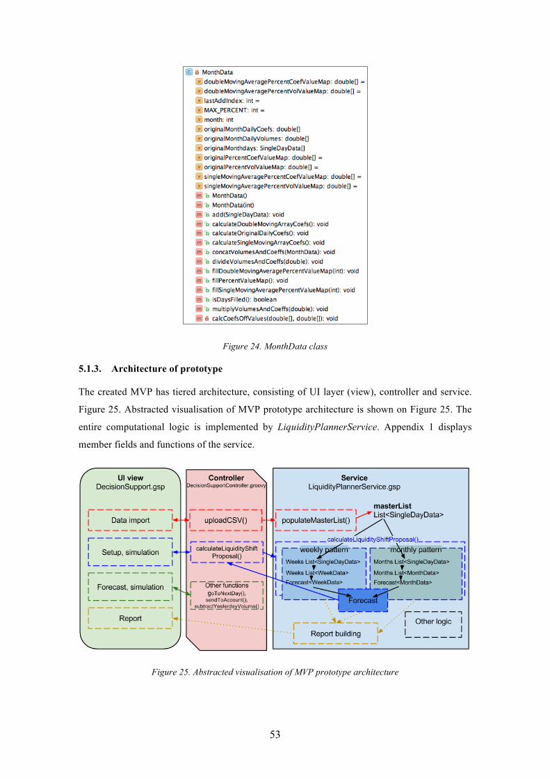
53

Figure 24. MonthData class

5.1.3. Architecture of prototype

The created MVP has tiered architecture, consisting of UI layer (view), controller and service.

Figure 25. Abstracted visualisation of MVP prototype architecture is shown on Figure 25. The

entire computational logic is implemented by LiquidityPlannerService. Appendix 1 displays

member fields and functions of the service.

Figure 25. Abstracted visualisation of MVP prototype architecture

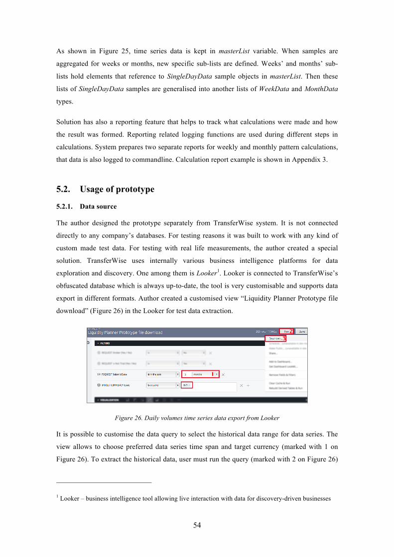
54

As shown in Figure 25, time series data is kept in masterList variable. When samples are

aggregated for weeks or months, new specific sub-lists are defined. Weeks’ and months’ sub-

lists hold elements that reference to SingleDayData sample objects in masterList. Then these

lists of SingleDayData samples are generalised into another lists of WeekData and MonthData

types.

Solution has also a reporting feature that helps to track what calculations were made and how

the result was formed. Reporting related logging functions are used during different steps in

calculations. System prepares two separate reports for weekly and monthly pattern calculations,

that data is also logged to commandline. Calculation report example is shown in Appendix 3.

5.2. Usage of prototype

5.2.1. Data source

The author designed the prototype separately from TransferWise system. It is not connected

directly to any company’s databases. For testing reasons it was built to work with any kind of

custom made test data. For testing with real life measurements, the author created a special

solution. TransferWise uses internally various business intelligence platforms for data

exploration and discovery. One among them is Looker1. Looker is connected to TransferWise’s

obfuscated database which is always up-to-date, the tool is very customisable and supports data

export in different formats. Author created a customised view “Liquidity Planner Prototype file

download” (Figure 26) in the Looker for test data extraction.

Figure 26. Daily volumes time series data export from Looker

It is possible to customise the data query to select the historical data range for data series. The

view allows to choose preferred data series time span and target currency (marked with 1 on

Figure 26). To extract the historical data, user must run the query (marked with 2 on Figure 26)

1 Looker – business intelligence tool allowing live interaction with data for discovery-driven businesses

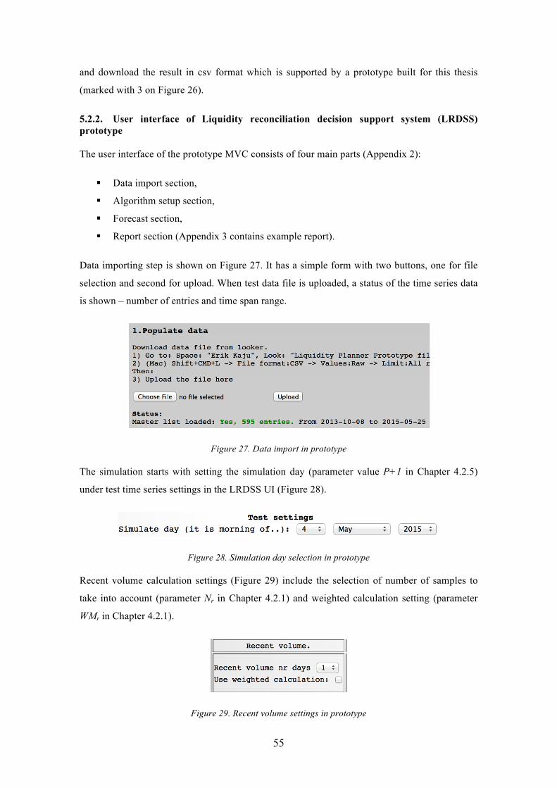
55

and download the result in csv format which is supported by a prototype built for this thesis

(marked with 3 on Figure 26).

5.2.2. User interface of Liquidity reconciliation decision support system (LRDSS) prototype

The user interface of the prototype MVC consists of four main parts (Appendix 2):

§ Data import section,

§ Algorithm setup section,

§ Forecast section,

§ Report section (Appendix 3 contains example report).

Data importing step is shown on Figure 27. It has a simple form with two buttons, one for file

selection and second for upload. When test data file is uploaded, a status of the time series data

is shown – number of entries and time span range.

Figure 27. Data import in prototype

The simulation starts with setting the simulation day (parameter value P+1 in Chapter 4.2.5)

under test time series settings in the LRDSS UI (Figure 28).

Figure 28. Simulation day selection in prototype

Recent volume calculation settings (Figure 29) include the selection of number of samples to

take into account (parameter Nr in Chapter 4.2.1) and weighted calculation setting (parameter

WMr in Chapter 4.2.1).

Figure 29. Recent volume settings in prototype

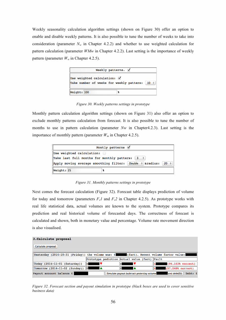
56

Weekly seasonality calculation algorithm settings (shown on Figure 30) offer an option to

enable and disable weekly patterns. It is also possible to tune the number of weeks to take into

consideration (parameter Nw in Chapter 4.2.2) and whether to use weighted calculation for

pattern calculation (parameter WMw in Chapter 4.2.2). Last setting is the importance of weekly

pattern (parameter Ww in Chapter 4.2.5).

Figure 30. Weekly patterns settings in prototype

Monthly pattern calculation algorithm settings (shown on Figure 31) also offer an option to

exclude monthly patterns calculation from forecast. It is also possible to tune the number of

months to use in pattern calculation (parameter Nw in Chapter4.2.3). Last setting is the

importance of monthly pattern (parameter Wm in Chapter 4.2.5).

Figure 31. Monthly patterns settings in prototype

Next comes the forecast calculation (Figure 32). Forecast table displays prediction of volume

for today and tomorrow (parameters Fv1 and Fv2 in Chapter 4.2.5). As prototype works with

real life statistical data, actual volumes are known to the system. Prototype compares its

prediction and real historical volume of forecasted days. The correctness of forecast is

calculated and shown, both in monetary value and percentage. Volume rate movement direction

is also visualised.

Figure 32. Forecast section and payout simulation in prototype (black boxes are used to cover sensitive business data)

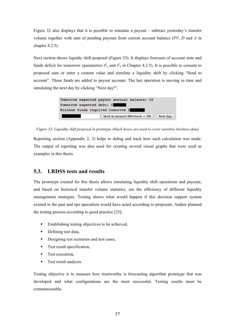
57

Figure 32 also displays that it is possible to simulate a payout – subtract yesterday’s transfer

volume together with sum of pending payouts from current account balance (PV, D and A in

chapter 4.2.5).

Next section shows liquidty shift proposal (Figure 33). It displays forecasts of account state and

funds deficit for tomorrow (parameters Fa and Fd in Chapter 4.2.5). It is possible to consent to

proposed sum or enter a custom value and simulate a liquidity shift by clicking “Send to

account”. These funds are added to payout account. The last operation is moving in time and

simulating the next day by clicking “Next day!”.

Figure 33. Liquidity shift proposal in prototype (black boxes are used to cover sensitive business data)

Reporting section (Appendix 2, 3) helps to debug and track how each calculation was made.

The output of reporting was also used for creating several visual graphs that were used as

examples in this thesis.

5.3. LRDSS tests and results

The prototype created for this thesis allows simulating liquidity shift operations and payouts,

and based on historical transfer volume statistics, see the efficiency of different liquidity

management strategies. Testing shows what would happen if this decision support system

existed in the past and ops specialists would have acted according to proposals. Author planned

the testing process according to good practice [25]:

§ Establishing testing objectives to be achieved,

§ Defining test data,

§ Designing test scenarios and test cases,

§ Test result specification,

§ Test execution,

§ Test result analysis.

Testing objective is to measure how trustworthy is forecasting algorithm prototype that was

developed and what configurations are the most successful. Testing results must be

commensurable.

58

One part of test data is data series, it must be similar when testing different algorithm

configurations. Algorithms under test must be in equal conditions, then it is possible to justify

the difference in results. So time span used in test is always the same. Another part of test data

is different combinations of forecast algorithm settings. Different scenarios must be tested out.

There is only one test case and it is carried out against different algorithm settings. Different

settings scenarios can be seen in Table 11. Common test steps are following:

1. Calculate proposal,

2. Consent to the sum proposed by prototype and shift liquidity according to proposal,

3. Simulate payouts,

4. Go to next day,

5. Repeat steps 1-4 for n consequent days.

Test results are compared based on predefined specifications. For every simulation day under

test, a set of interim results will be logged:

§ how big was the forecast fault,

§ whether forecast guesses volume rate movement direction correctly,

§ whether the payout account runs out of money and liquidity deficit situation arises.

For each scenario under test, a set of results’ info is summed up. Test summaries are compared

in test result matrix table. It is also important to record how big overdepreciation or deficit of

funds is on payout account in by the end of testcase execution.

All tests start in harsh conditions with zero amount on account. It means that testcase starts with

payout funds deficit equal to the volume of one whole day. Algorithm must cope with crisis

situation and normalise the account state. Test results based on 5 different scenarios and making

up 150 test executions (Table 12), reveal that as expected, differences in forecasting algorithm

configuration cause notable precision divergence.

According to Eric Ries, a minimum viable product is such version of a new product which

allows to collect the maximum amount of validated learning with the least effort [4]. It is the

smallest thing to build that delivers value. Author analysed various determinants that affect

transfer volumes and picked for implementation the ones which are directly related to time

series analysis and, based on observations, have the greatest significance.

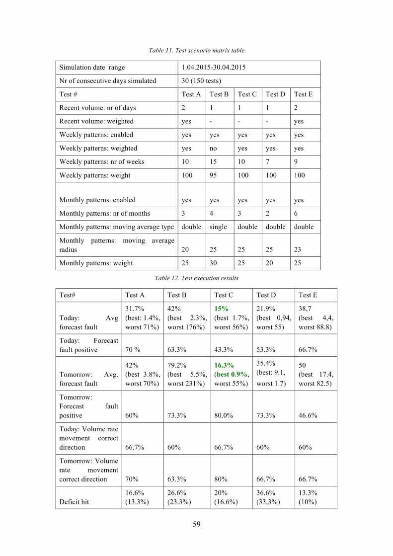
59

Table 11. Test scenario matrix table

Simulation date range 1.04.2015-30.04.2015

Nr of consecutive days simulated 30 (150 tests)

Test # Test A Test B Test C Test D Test E

Recent volume: nr of days 2 1 1 1 2

Recent volume: weighted yes - - - yes

Weekly patterns: enabled yes yes yes yes yes

Weekly patterns: weighted yes no yes yes yes

Weekly patterns: nr of weeks 10 15 10 7 9

Weekly patterns: weight 100 95 100 100 100

Monthly patterns: enabled yes yes yes yes yes

Monthly patterns: nr of months 3 4 3 2 6

Monthly patterns: moving average type double single double double double

Monthly patterns: moving average radius 20 25 25 25 23

Monthly patterns: weight 25 30 25 20 25

Table 12. Test execution results

Test# Test A Test B Test C Test D Test E

Today: Avg forecast fault

31.7% (best: 1.4%, worst 71%)

42% (best 2.3%, worst 176%)

15% (best 1.7%, worst 56%)

21.9% (best 0,94, worst 55)

38,7 (best 4,4, worst 88.8)

Today: Forecast fault positive 70 % 63.3% 43.3% 53.3% 66.7%

Tomorrow: Avg. forecast fault

42% (best 3.8%, worst 70%)

79.2% (best 5.5%, worst 231%)

16.3% (best 0.9%, worst 55%)

35.4% (best: 9.1, worst 1.7)

50 (best 17.4, worst 82.5)

Tomorrow: Forecast fault positive 60% 73.3% 80.0% 73.3% 46.6%

Today: Volume rate movement correct direction 66.7% 60% 66.7% 60% 60%

Tomorrow: Volume rate movement correct direction 70% 63.3% 80% 66.7% 66.7%

Deficit hit 16.6% (13.3%)

26.6% (23.3%)

20% (16.6%)

36.6% (33,3%)

13.3% (10%)

60

Taking into consideration that the prototype does not include in computation all factors,

building absolutely faultless system was not the expectation. The idea was to build a MVP,

carry out a series of tests and assess how auspicious the concept is. Testing shows that some

configurations result more optimistic forecasts and others rather pessimistic – for instance, in

70% of cases the test scenario A forecasted higher volume for upcoming day than it really

turned out to be while Test C was more pessimistic in 56,7% of attempts. Regarding next day’s

prediction, Test C showed the most optimistic forecasts, while Test E predicted too little volume

in 53.4% of attempts. The best combination’s forecasting misses the reality by ~15%, it means

that the average prediction correctness is 85% (pure volume forecasting, without additional

buffer that is added in proposal calculation) where both inadequate and excessive forecasts are

treated as fault. From business operational point of view, insufficient liquidity transfer is more

deprecated. The test scenario C with the greatest precision, in majority of cases also forecasts

correctly whether the volume will grow or decline next day – 80% of executed tests forecasted

the volume rate movement direction correctly, the reliability of analogous forecast for next day

was also 80%. Based on that, the algorithm setup used in Test C is definitely the most reliable in

terms of forecast precision and it tells quite reliably whether the daily volumes will grow or

decline in the next two days. In terms of proposal calculation, it evidently needs improvement,

because even in test scenarios with relatively high forecasting precision, funds deficit situations

occur. From proposal perspective, the most successful was Test E – after normalising the

account state, in 90% of days under test, the deficit occasion did not occur. Proposal algorithm

can be enhanced by increasing the risk mitigation buffer size logic. For some days, the

precision of forecasts is very high, faults are less than 1%. But at the same time, some less

successful predictions have serious imperfections. Author finds that this unstability factor

comes from the fact that not complete scope of functionality is implemented in MVP. Author

assumes that including more factors into calculations and using smarter algorithms in time

series analysis will significantly improve the accuracy and stability of correct forecasts. Author

finds that the MVP has potential because the results in Test scenario C are good for a prototype

with minimal features. Author proposes that the next reasonable step is to enhance the proposal

feature, implement at one or two of several remaining factors in order of their significance and

then to compare the precision and reliability with current human factor. If decision support

system is less efficient than operations specialists, then implement one more determinant and

repeat the test. Once test results will show that decision making assistant tool is more accurate

than human being today, then the solution is ready to be launched in live environment. That

version will be minimum viable product that is reliable in real life and any further enhancements

and improvements will only make it better.

61

6. Conclusions

The objective of this thesis was to use information technology facilities and build a minimum

viable product solution that would potentially enhance a liquidity planning process in the

world’s fastest growing money transfer service. The thesis gives an overview about the

remittance business. Within scope of this thesis, the author designed and built a prototype of

decision support system for making liquidity balancing decisions based on historical data of

fund flows. The prototype focuses on remittance channel to Indian rupee. System forecasts

future transfer volumes and makes proposals when it is the right time to buy certain currency

and how much company should buy that. The difficulty of forecasting lies in the fact of rapidly

changing environment, randomness and, most notably, the diversity of factors that influence the

demand for money. Author made a research on factors that impact transfer volumes. The

analysis of these determinants covers characteristics, impact and significance.

In the thesis a computational model for transfer volumes’ forecasting calculations was

established and implemented in a prototype tool for decision support system. It is explained in

detail how indications from selected problem factors are used in forecast calculations. Author

describes the implementation and architecture of the solution – how computational model is

realised and programmed, which data structures are used and how to use it.

Author tested the solution with real historical data and analysed the results. The idea was to

implement the minimal required features, carry out a series of tests and assess how auspicious

the concept is. Testing shows that in majority of cases, the concept is able to forecast correctly

whether the volume will grow or decline over next days. Author finds that the MVP has

potential because the results in one of executed test scenarios are good for a prototype with

minimal set of functionalities. For some days the precision of forecasts is very high (faults are

less than 1%) while some other less successful predictions have notable imperfections. Author

assumes that including more factors into calculations and using smarter sophisticated algorithms

for time series analysis will improve the accuracy and stability of correct forecasts.

On the average, predictions are quite accurate, but there is still some unstability factor that could

be reduced. Therefore, author proposes that the next reasonable step is to enhance the proposal

feature, implement one or a couple of several remaining factors in order of their significance

and then compare the precision and reliability with current human factor. If decision support

system is less efficient, implement one more determinant and repeat the test. Once tests will

show that decision making assistant tool is more accurate than human being today, then the

62

solution is ready to be launched in live environment. As the number of connected determinants

grows, the overall complexity of the algorithm together with every new enhancement will

ascend as well. Building the whole necessary logic completely from scratch is a tremendous

task of high complexity. In order to efficiently ease the future improvement task, it might be

reasonable to build a hybrid solution and perform some parts of calculations in 3rd party data

analysis tools. Such approach can save valuable development time. Author finds that further

development of the solution in longer term is reasonable and encouraged but for the best results

requires deep research in time series analysis subject field. Stable and trustworthy decision

support system can be very beneficial for the company – it saves human resources and helps to

mitigate businesses FX and enterprise risks which in turn helps to save real financial assets of

the company.

63

References

1. Alistair Graham and Brian Coyle, Cash Flow Forecasting and Liquidity. Chicago, USA: Fitzroy Dearborn Publishers, 2000.

2. Dmitris Chorafas, Liabilities, Liquidity, and Cash Management: Balancing Financial Risks. New York, USA: John Wiley & Sons, 2002.

3. Alastair Hudson, Equity and Trusts. New York, USA: Routledge, 2014. 4. Eric Ries, The Lean Startup: How Today's Entrepreneurs Use Continuous Innovation to Create

Radically Successful Businesses. New York, USA: Crown Publishing Group, 2011. 5. Ann-Marii Nergi, "Kristo Käärmann: 8M from dollars to euros has been the biggest transaction

so far," Eesti Päevaleht, May 2015. 6. Bharati Basu and James Bang, International Remittance Payments and the Global Economy.

New York, USA: Routledge, 2015. 7. Jonathan Moules. (2013, May) The Financial Times. [WWW]

http://www.ft.com/intl/cms/s/0/9d1b4290-bbcf-11e2-82df-00144feab7de.html 8. Sally Davies. (2014, June) The Financial Times. [Online]. [WWW]

http://www.ft.com/intl/cms/s/0/9d1665b6-efec-11e3-a943-00144feabdc0.html 9. Sophie Curtis. (2015, Jan.) The Telegraph. [WWW]

http://www.telegraph.co.uk/technology/news/11369204/TransferWise-attracts-58m-in-funding-from-Andreessen-Horowitz.html

10. UK Information Commissioner's Office, Data Protection Act 1998: Information Commissioner's Guidance about the Issue of Monetary Penalties Prepared and Issued Under Section 55C (1) of the Data Protection Act 1998. UK: Crown, 2012.

11. TransferWise Ltd. TransferWise: Security. [WWW] https://transferwise.com/security 12. Eric Rescorla, SSL and TLS: Designing and Building Secure Systems. Boston, USA: Addison-

Wesley, 2002. 13. OECD, OECD Glossary of Statistical Terms. Paris, France: OECD Publications, 2008. 14. Chris Chatfield, The Analysis of Time Series, 6th ed. London: Chapman and Hall/CRC , 2013. 15. Robert Yaffe and Monnie McGee, An Introduction to Time Series Analysis and Forecasting.

New York, USA: Academic Press, 2000. 16. Vijay Mishra, The Literature of the Indian Diaspora: Theorizing the Diasporic Imaginary.

Abingdon, UK: Routledge, 2007. 17. Morgan Kaufmann, Data Mining: Burlington, USA: M. Kaufmann Publishers, 2008. 18. Government of India, "Holidays to be observed in Central Government Offices to the year

2015," Ministry of Personnel, Public Grievances and Pensions, New Delhi, 2014. 19. Ioannis Christou, Quantitative Methods in Supply Chain Management: Models and Algorithms.

Athens, Greece: Springer Science & Business Media, 2011. 20. Mark Filler and James DiGabriele , A Quantitative Approach to Commercial Damages:

Applying Statistics to the Measurement of Lost Profits. New Jersey, USA: J.Wiley&Sons, 2012. 21. Naval Bajpai, Business Statistics. New Delhi, India: Pearson Education, 2009. 22. J.P.Chauhan, Computer Oriented Statistical and Optimization Methods, 3rd ed.: Pragati

Prakashan-Meerut, 2010. 23. Kenneth Barclay and John Savage, Groovy Programming: An Introduction for Java Developers.

San Francisco, USA: Morgan Kaufmann Publishers, 2010. 24. Graeme Rocher, The Definitive Guide to Grails. New York, USA: Apress, 2006. 25. Milind Limaye, Software Testing. New Delhi, India: Tata McGraw-Hill Education, 2009.

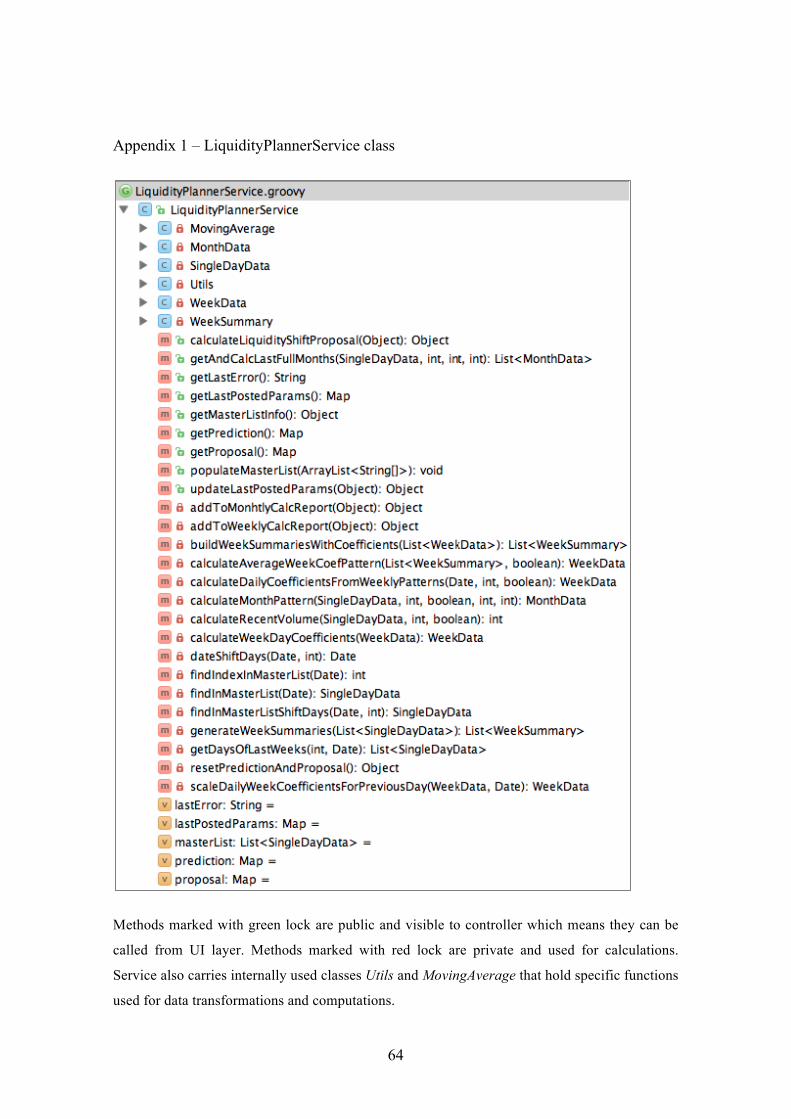
64

Appendix 1 – LiquidityPlannerService class

Methods marked with green lock are public and visible to controller which means they can be

called from UI layer. Methods marked with red lock are private and used for calculations.

Service also carries internally used classes Utils and MovingAverage that hold specific functions

used for data transformations and computations.

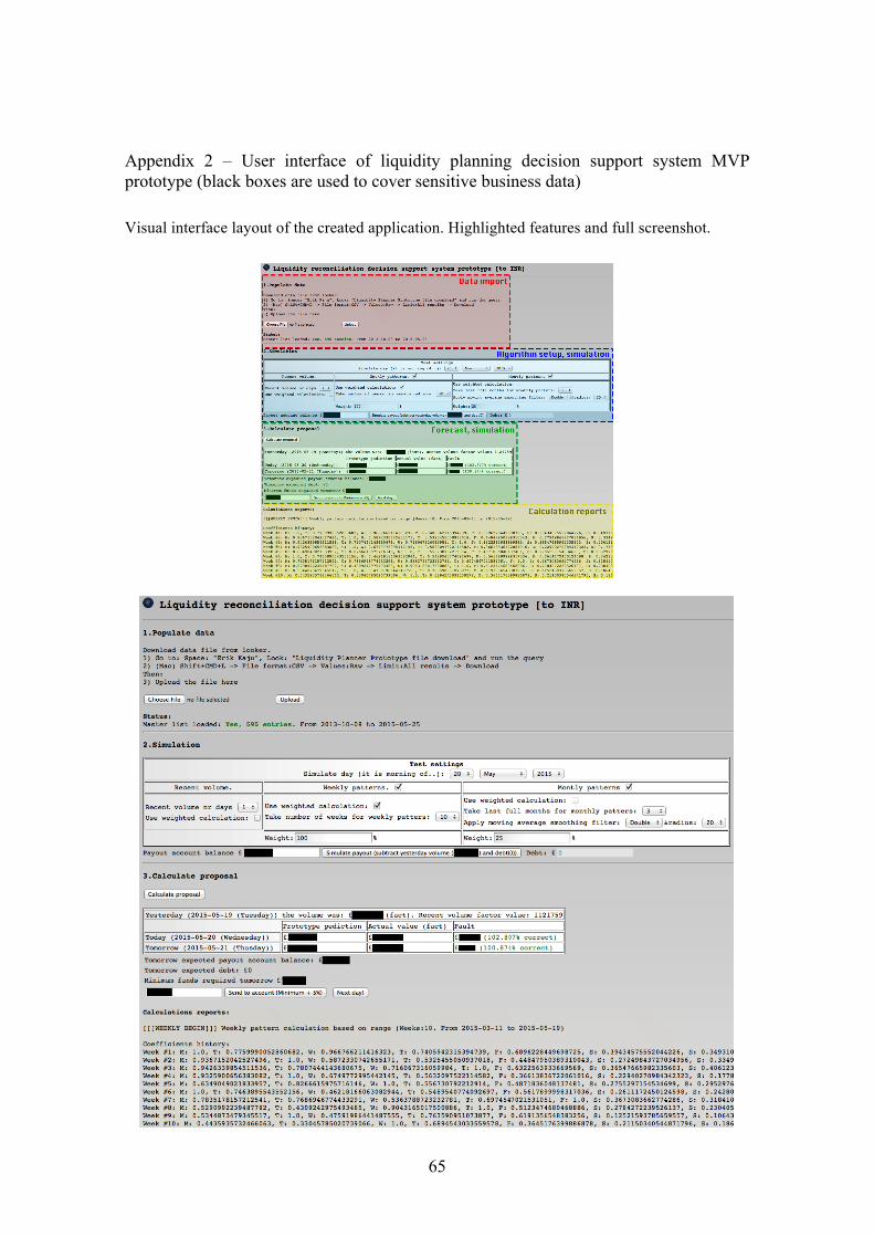
65

Appendix 2 – User interface of liquidity planning decision support system MVP prototype (black boxes are used to cover sensitive business data)

Visual interface layout of the created application. Highlighted features and full screenshot.

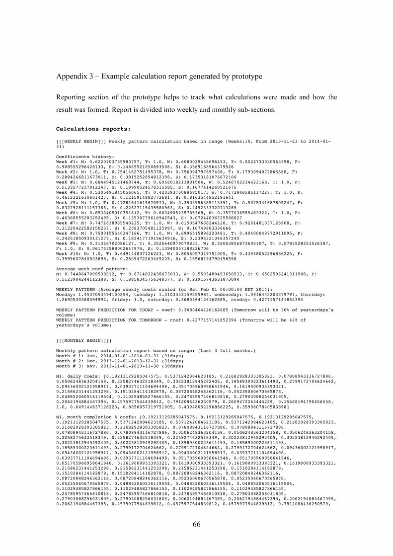
66

Appendix 3 – Example calculation report generated by prototype

Reporting section of the prototype helps to track what calculations were made and how the

result was formed. Report is divided into weekly and monthly sub-sections.

Calculations reports: [[[WEEKLY BEGIN]]] Weekly pattern calculation based on range (Weeks:10. From 2013-11-23 to 2014-01-31) Coefficients history: Week #1: M: 0.6220203755983797, T: 1.0, W: 0.6080029458696453, T: 0.5524733030563398, F: 0.908555296428133, S: 0.14665521050693506, S: 0.3569166564379526 Week #2: M: 1.0, T: 0.7541462751495378, W: 0.756094797897408, T: 0.1793094072865688, F: 0.2884266811673011, S: 0.3815252854812398, S: 0.17353181076672106 Week #3: M: 0.6844945121469744, T: 0.6956018213881504, W: 0.5240702234622168, T: 1.0, F: 0.5133577237912247, S: 0.19990524570315585, S: 0.1677414260521675 Week #4: M: 0.5305491845056065, T: 0.42039373088685017, W: 0.7172846585117227, T: 1.0, F: 0.4612321610601427, S: 0.1215914882772681, S: 0.8163544852191641 Week #5: M: 1.0, T: 0.47281641615870973, W: 0.3503956385113391, T: 0.5075341687805247, F: 0.8327528111157385, S: 0.22627115435580963, S: 0.2492333320713285 Week #6: M: 0.8533405010751612, T: 0.6034905235785368, W: 0.3577036555483322, T: 1.0, F: 0.40368555283292495, S: 0.13530779616942543, S: 0.07244836725508827 Week #7: M: 0.7471838965540225, T: 1.0, W: 0.6150547668244128, T: 0.9261481037125908, F: 0.31220422582150237, S: 0.2583705481125997, S: 0.16749983336666 Week #8: M: 0.7500155540347166, T: 1.0, W: 0.6996515896223481, T: 0.40400049772911095, F: 0.24251850930131277, S: 0.18241771915634916, S: 0.2395321346357245 Week #9: M: 0.31326702086127, T: 0.3526640979070833, W: 0.26063856873695107, T: 0.5783528253526387, F: 1.0, S: 0.061743588002647974, S: 0.13940047188226706 Week #10: M: 1.0, T: 0.649144837126223, W: 0.8056057319751005, T: 0.43948052296886225, F: 0.3599607840503898, S: 0.2609472263445229, S: 0.15568194790456558 Average week coef pattern: M: 0.7448647009530912, T: 0.6714022438673033, W: 0.5593480453650533, T: 0.6502506241311908, F: 0.5123904244112388, S: 0.18858345756348377, S: 0.21915743631873094 WEEKLY PATTERN (Average weekly coefs scaled for Sat Feb 01 00:00:00 EET 2014): Monday: 1.4537053494100254, tuesday: 1.3103333159255985, wednesday: 1.0916442203379797, thursday: 1.2690530368094992, friday: 1.0, saturday: 0.3680464126162685, sunday: 0.4277157141852394 WEEKLY PATTERN PREDICTION FOR TODAY - coef: 0.3680464126162685 (Tomorrow will be 36% of yesterdays's volume) WEEKLY PATTERN PREDICTION FOR TOMORROW - coef: 0.4277157141852394 (Tomorrow will be 42% of yesterdays's volume) [[[MONTHLY BEGIN]]]] Monthly pattern calculation report based on range: (Last 3 full months.) Month # 1: Jan, 2014-01-01-2014-01-31 (31days) Month # 2: Dec, 2013-12-01-2013-12-31 (31days) Month # 3: Nov, 2013-11-01-2013-11-30 (30days) M1, daily coefs: [0.19213129285047575, 0.5371242084623185, 0.21682928303305823, 0.07808943116727886, 0.0506248363204158, 0.2258274632518349, 0.30223812945292405, 0.18589300223611493, 0.2799172704624662, 0.09436002121958917, 0.03937711104694498, 0.051705960958641946, 0.1619000933393321, 0.21586231441253298, 0.1510284114182878, 0.08720848246362116, 0.05235060670565878, 0.048852060516119504, 0.11029485827866155, 0.24785957466810818, 0.27903088256031805, 0.2062194884467395, 0.4575977544839812, 0.7912086436250579, 0.2609472263445229, 0.15568194790456558, 1.0, 0.649144837126223, 0.8056057319751005, 0.43948052296886225, 0.3599607840503898] M1, month completion % coefs: [0.19213129285047575, 0.19213129285047575, 0.19213129285047575, 0.19213129285047575, 0.5371242084623185, 0.5371242084623185, 0.5371242084623185, 0.21682928303305823, 0.21682928303305823, 0.21682928303305823, 0.07808943116727886, 0.07808943116727886, 0.07808943116727886, 0.07808943116727886, 0.0506248363204158, 0.0506248363204158, 0.0506248363204158, 0.2258274632518349, 0.2258274632518349, 0.2258274632518349, 0.30223812945292405, 0.30223812945292405, 0.30223812945292405, 0.30223812945292405, 0.18589300223611493, 0.18589300223611493, 0.18589300223611493, 0.2799172704624662, 0.2799172704624662, 0.2799172704624662, 0.09436002121958917, 0.09436002121958917, 0.09436002121958917, 0.09436002121958917, 0.03937711104694498, 0.03937711104694498, 0.03937711104694498, 0.051705960958641946, 0.051705960958641946, 0.051705960958641946, 0.1619000933393321, 0.1619000933393321, 0.1619000933393321, 0.1619000933393321, 0.21586231441253298, 0.21586231441253298, 0.21586231441253298, 0.1510284114182878, 0.1510284114182878, 0.1510284114182878, 0.08720848246362116, 0.08720848246362116, 0.08720848246362116, 0.08720848246362116, 0.05235060670565878, 0.05235060670565878, 0.05235060670565878, 0.048852060516119504, 0.048852060516119504, 0.048852060516119504, 0.11029485827866155, 0.11029485827866155, 0.11029485827866155, 0.11029485827866155, 0.24785957466810818, 0.24785957466810818, 0.24785957466810818, 0.27903088256031805, 0.27903088256031805, 0.27903088256031805, 0.2062194884467395, 0.2062194884467395, 0.2062194884467395, 0.2062194884467395, 0.4575977544839812, 0.4575977544839812, 0.4575977544839812, 0.7912086436250579,

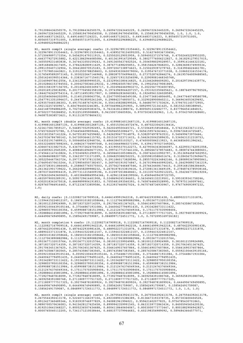
67

0.7912086436250579, 0.7912086436250579, 0.2609472263445229, 0.2609472263445229, 0.2609472263445229, 0.2609472263445229, 0.15568194790456558, 0.15568194790456558, 0.15568194790456558, 1.0, 1.0, 1.0, 0.649144837126223, 0.649144837126223, 0.649144837126223, 0.649144837126223, 0.8056057319751005, 0.8056057319751005, 0.8056057319751005, 0.43948052296886225, 0.43948052296886225, 0.43948052296886225] M1, month compl% (single average) coefs: [0.32296789115354463, 0.32296789115354463, 0.32296789115354463, 0.32296789115354463, 0.43895278124095205, 0.5162760036730656, 0.5715069897173354, 0.5456291479311915, 0.5255020129053959, 0.5094002371576748, 0.47502445229953205, 0.4463779272915882, 0.42213862944085084, 0.4013619916729549, 0.38027776006212827, 0.3618291279517015, 0.3455509231483838, 0.3474431050159243, 0.34913605637602524, 0.3506598029028957, 0.3599141446323181, 0.3691684863617405, 0.3784228280911629, 0.3876771698205853, 0.3581566267848203, 0.32863608374905534, 0.2991155407132904, 0.3044180070515183, 0.30972047338974623, 0.3150229397279742, 0.3163904624461781, 0.3177579851643821, 0.31912550788258603, 0.32049303060079004, 0.3195476733771038, 0.3186023161534176, 0.31765695892973145, 0.3030222647146968, 0.2883875704996622, 0.2737528762846276, 0.26195764009488565, 0.25016240390514366, 0.23836716771540176, 0.2265719315256598, 0.22909081468345768, 0.2316096978412556, 0.2341285809990535, 0.22329563380416825, 0.212462686609283, 0.20162973941439774, 0.20102866153784502, 0.20042758366129232, 0.1998265057847396, 0.1992254279081869, 0.20031583397156705, 0.20140624003494717, 0.2024966460983273, 0.20225677934007855, 0.2020169125818298, 0.20177704582358108, 0.19743969044207157, 0.1931023350605621, 0.1887649796790526, 0.18442762429754314, 0.1871169539517907, 0.1898062836060383, 0.19249561326028589, 0.20325406066202095, 0.214012508063756, 0.22477095546549108, 0.2347736814806495, 0.24477640749580798, 0.25477913351096637, 0.2647818595261249, 0.298842374805073, 0.3329028900840211, 0.3669634053629692, 0.4293575465186303, 0.49175168767429134, 0.5541458288299524, 0.566807971703624, 0.5794701145772955, 0.592132257450967, 0.6047944003246385, 0.5970469862293905, 0.5892995721341425, 0.5815521580388945, 0.6421487094886209, 0.7027452609383474, 0.763341812388074, 0.8005691332682777, 0.8377964541484815, 0.8750237750286852, 0.912251095908889, 0.941500730605926, 0.970750365302963, 1.0, 0.970437691928681, 0.9408753838573621, 0.9113130757860433] M1, month compl% (double average) coefs: [0.41998816012687135, 0.41998816012687135, 0.41998816012687135, 0.41998816012687135, 0.4501535616572476, 0.48702230420136416, 0.5236175817859127, 0.5468575529392493, 0.5620249500445721, 0.5720649158548466, 0.5762156236711152, 0.576570262072788, 0.5744456609859446, 0.5706946553086477, 0.5656159574363461, 0.5596726816725487, 0.5531833567141226, 0.5475518574259682, 0.5426290477914879, 0.5382974978763531, 0.540699673970466, 0.5437036784780142, 0.5473093646115792, 0.5515167323711615, 0.5462635042589635, 0.5340631212318753, 0.5163521917489913, 0.5006685432948756, 0.486638455103527, 0.4740000584213923, 0.4636856001396242, 0.45532268057898245, 0.4486247706997048, 0.44336669860271594, 0.43941797027349283, 0.4366074315827515, 0.43479372624704354, 0.4319055370122273, 0.42795563438366097, 0.4229551742051058, 0.4165859213545309, 0.40884816940677193, 0.39974177157441104, 0.3892667278574483, 0.3808747443880601, 0.3745661147410824, 0.3703406921290972, 0.36506603305388435, 0.3587424310902797, 0.35136944587602953, 0.3438686088207789, 0.3362397731371099, 0.3284829388250225, 0.32059810588451676, 0.31284567519496675, 0.3052256467563724, 0.29773787378131583, 0.2911860173828596, 0.28557022434842166, 0.2808903478905841, 0.2766954570615244, 0.27298540507382457, 0.2697601919274847, 0.26701996440992265, 0.2642908927361219, 0.26157283011866445, 0.2588657765575503, 0.2575627446487546, 0.2576634408174415, 0.2591681586384469, 0.2613621901739622, 0.2642458289988232, 0.26781878153819416, 0.2720813413669109, 0.27848743785938146, 0.2870373645904419, 0.29773112156009196, 0.3124972018648461, 0.33133575229212225, 0.3542467728419204, 0.37826324943600603, 0.40338488849954346, 0.4296118368199504, 0.45694409439722705, 0.4835979005289191, 0.5095729616401908, 0.5348694245184603, 0.5634065132219501, 0.5951839341758246, 0.6302018341675018, 0.6669899904191853, 0.7055481093560393, 0.7458764845528995, 0.7879751160097661, 0.8297607966916465, 0.8712336733859586, 0.9123937460927024, 0.9475748736930967, 0.9767769093997232, 1.0] M2, daily coefs: [0.11220827167909518, 0.6466149991942218, 0.4876422930981438, 0.4889022371331878, 0.11594415224812107, 0.18650101821058646, 0.11127063890882986, 0.0933677132015764, 0.3810012159924989, 0.3871837320714359, 0.2917063451367625, 0.5566169037607864, 0.2857435867383565, 0.055921004439105144, 0.375448671931084, 0.24400427794951435, 0.19334280733111622, 0.32988557950100356, 0.45990887381513984, 0.21212476376049344, 0.17511757035908404, 0.19288864145801896, 0.7739279487818099, 0.3659258391080768, 0.27118097777517325, 0.3927948781809924, 0.6444906749490895, 0.158562491759087, 0.08489971724511772, 1.0, 0.7072095169726182] M2, month completion % coefs: [0.11220827167909518, 0.11220827167909518, 0.11220827167909518, 0.11220827167909518, 0.6466149991942218, 0.6466149991942218, 0.6466149991942218, 0.4876422930981438, 0.4876422930981438, 0.4876422930981438, 0.4889022371331878, 0.4889022371331878, 0.4889022371331878, 0.4889022371331878, 0.11594415224812107, 0.11594415224812107, 0.11594415224812107, 0.18650101821058646, 0.18650101821058646, 0.18650101821058646, 0.11127063890882986, 0.11127063890882986, 0.11127063890882986, 0.11127063890882986, 0.0933677132015764, 0.0933677132015764, 0.0933677132015764, 0.3810012159924989, 0.3810012159924989, 0.3810012159924989, 0.3871837320714359, 0.3871837320714359, 0.3871837320714359, 0.3871837320714359, 0.2917063451367625, 0.2917063451367625, 0.2917063451367625, 0.5566169037607864, 0.5566169037607864, 0.5566169037607864, 0.2857435867383565, 0.2857435867383565, 0.2857435867383565, 0.2857435867383565, 0.055921004439105144, 0.055921004439105144, 0.055921004439105144, 0.375448671931084, 0.375448671931084, 0.375448671931084, 0.24400427794951435, 0.24400427794951435, 0.24400427794951435, 0.24400427794951435, 0.19334280733111622, 0.19334280733111622, 0.19334280733111622, 0.32988557950100356, 0.32988557950100356, 0.32988557950100356, 0.45990887381513984, 0.45990887381513984, 0.45990887381513984, 0.45990887381513984, 0.21212476376049344, 0.21212476376049344, 0.21212476376049344, 0.17511757035908404, 0.17511757035908404, 0.17511757035908404, 0.19288864145801896, 0.19288864145801896, 0.19288864145801896, 0.19288864145801896, 0.7739279487818099, 0.7739279487818099, 0.7739279487818099, 0.3659258391080768, 0.3659258391080768, 0.3659258391080768, 0.27118097777517325, 0.27118097777517325, 0.27118097777517325, 0.27118097777517325, 0.3927948781809924, 0.3927948781809924, 0.3927948781809924, 0.6444906749490895, 0.6444906749490895, 0.6444906749490895, 0.158562491759087, 0.158562491759087, 0.158562491759087, 0.158562491759087, 0.08489971724511772, 0.08489971724511772, 0.08489971724511772, 1.0, 1.0, 1.0] M2, month compl% (single average) coefs: [0.2675544392413178, 0.2675544392413178, 0.2675544392413178, 0.2675544392413178, 0.5224071166197104, 0.6923089015386389, 0.8136673193378735, 0.857303600404528, 0.8912427360489346, 0.9183939746977829, 0.940881961996021, 0.959621602077835, 0.9754785430701863, 0.9890700570636083, 0.9415628127625458, 0.8999942359991545, 0.8633159772863434, 0.8400594565420536, 0.8192510641568227, 0.8005236507434688, 0.8004118640604067, 0.8003000773773447, 0.8001882906942827, 0.8000765040112205, 0.7341171210038444, 0.6681577379964683, 0.602198354989092, 0.5894843664577071,

68

0.576770377926322, 0.5640563893949371, 0.5519292809496279, 0.5398021725043186, 0.5276750640590094, 0.5155479556137001, 0.5365027186870653, 0.5574574817604306, 0.5784122448337958, 0.622538291305616, 0.6666643377774363, 0.7107903842492563, 0.7315914406334113, 0.7523924970175663, 0.7731935534017212, 0.793994609785876, 0.7895301291310856, 0.7850656484762951, 0.7806011678215046, 0.7799391810577465, 0.7792771942939885, 0.7786152075302304, 0.7615450316932714, 0.7444748558563121, 0.7274046800193531, 0.710334504182394, 0.698607382462416, 0.6868802607424381, 0.6751531390224604, 0.6481217217245191, 0.621090304426578, 0.5940588871286367, 0.614823263507412, 0.6355876398861872, 0.6563520162649624, 0.6771163926437376, 0.6957393553751055, 0.7143623181064733, 0.7329852808378412, 0.7091013573348658, 0.6852174338318903, 0.6613335103289149, 0.6552393894351104, 0.649145268541306, 0.6430511476475017, 0.6369570267536973, 0.7061756902391012, 0.7753943537245053, 0.8446130172099091, 0.8489098178401066, 0.853206618470304, 0.8575034191005014, 0.8350028558004188, 0.8125022925003362, 0.7900017292002536, 0.767501165900171, 0.7890410623926891, 0.8105809588852073, 0.8321208553777254, 0.888080570251817, 0.9440402851259084, 1.0, 0.9959075593997754, 0.9918151187995508, 0.9877226781993261, 0.9836302375991014, 0.9014827455508027, 0.8193352535025038, 0.7371877614542051, 0.8127835058749142, 0.8883792502956234, 0.9639749947163325] M2, month compl% (double average) coefs: [0.30485329308426035, 0.30485329308426035, 0.30485329308426035, 0.30485329308426035, 0.36292945744950156, 0.4339114361181297, 0.5043668174414772, 0.5634229384689112, 0.6136522849468785, 0.6569295911885099, 0.6946674754692408, 0.7278952505138603, 0.7574006231600935, 0.7837973599282904, 0.8030657279461986, 0.816965430058479, 0.8267713652046126, 0.8340155614888972, 0.8392496923206743, 0.8428932842320116, 0.8732500489580298, 0.9036008431926048, 0.9339452689029738, 0.964283326089137, 0.9763445148697079, 0.9749685156084568, 0.9629208599418235, 0.9476634680753842, 0.9297476153857176, 0.9095609857838618, 0.8874021038419714, 0.863485111186472, 0.8379735992829042, 0.8109969287792017, 0.7879201832861267, 0.768405831020763, 0.7521748510163369, 0.7397824989770558, 0.7310894634359143, 0.7259775286623392, 0.7220569059480423, 0.7193275952930237, 0.7177895966972834, 0.7174429101608212, 0.7206001060359281, 0.7272603882570782, 0.7374237568242716, 0.7482741299401836, 0.759811109572051, 0.772034695719874, 0.783976474671583, 0.7956368444599411, 0.8070154070521852, 0.8181125604810784, 0.8273477166452524, 0.8347208755447078, 0.8402324352122071, 0.8416896331570844, 0.8390932654448652, 0.8324429340427869, 0.8257906124768941, 0.819136300747187, 0.8124799988536656, 0.8058213087635668, 0.8004781169547628, 0.7964500253944902, 0.7937374321155122, 0.7897017779327451, 0.784343062846189, 0.7776616848886065, 0.7716052183687344, 0.7661744593520982, 0.7613686117731723, 0.7571880736647194, 0.7576195411796735, 0.7626622182525088, 0.772316502915988, 0.7837551684554259, 0.7969790109363482, 0.811987632325992, 0.8245312368151647, 0.8346102224366292, 0.8422241911576225, 0.8473735410109077, 0.8526888705263108, 0.8581705777365946, 0.8638182646089964, 0.8740146698955085, 0.8887597935961304, 0.9080540337436255, 0.9274621112613022, 0.9469840261491603, 0.966620176439963, 0.9863701641009475, 0.997496771954293, 1.0, 0.9938798482380681, 0.9918220188540158, 0.9938257157823174, 0.9998913370557357] M3, daily coefs: [0.2104578372407021, 0.06903154535411808, 0.006358168651037192, 0.6814287467779551, 0.27951393150853077, 0.6966490732785074, 0.3041855897876519, 0.2755615564011292, 0.23019516386399902, 0.11493801399288081, 0.3187185467043083, 0.38910028231250765, 0.34397937891248315, 0.6212348103596416, 0.19540935313612373, 0.01406652755615564, 0.4802258500061372, 0.30882533447894933, 0.1178102368970173, 0.35426537375721123, 0.7260095740763471, 0.392267092181171, 0.14665521050693506, 0.3569166564379526, 0.6220203755983797, 1.0, 0.6080029458696453, 0.5524733030563398, 0.908555296428133, 0.4133791579722597] M3, month completion % coefs: [0.2104578372407021, 0.2104578372407021, 0.2104578372407021, 0.2104578372407021, 0.06903154535411808, 0.06903154535411808, 0.06903154535411808, 0.006358168651037192, 0.006358168651037192, 0.006358168651037192, 0.006358168651037192, 0.6814287467779551, 0.6814287467779551, 0.6814287467779551, 0.27951393150853077, 0.27951393150853077, 0.27951393150853077, 0.27951393150853077, 0.6966490732785074, 0.6966490732785074, 0.6966490732785074, 0.3041855897876519, 0.3041855897876519, 0.3041855897876519, 0.3041855897876519, 0.2755615564011292, 0.2755615564011292, 0.2755615564011292, 0.23019516386399902, 0.23019516386399902, 0.23019516386399902, 0.23019516386399902, 0.11493801399288081, 0.11493801399288081, 0.11493801399288081, 0.3187185467043083, 0.3187185467043083, 0.3187185467043083, 0.38910028231250765, 0.38910028231250765, 0.38910028231250765, 0.38910028231250765, 0.34397937891248315, 0.34397937891248315, 0.34397937891248315, 0.6212348103596416, 0.6212348103596416, 0.6212348103596416, 0.6212348103596416, 0.19540935313612373, 0.19540935313612373, 0.19540935313612373, 0.01406652755615564, 0.01406652755615564, 0.01406652755615564, 0.01406652755615564, 0.4802258500061372, 0.4802258500061372, 0.4802258500061372, 0.30882533447894933, 0.30882533447894933, 0.30882533447894933, 0.30882533447894933, 0.1178102368970173, 0.1178102368970173, 0.1178102368970173, 0.35426537375721123, 0.35426537375721123, 0.35426537375721123, 0.7260095740763471, 0.7260095740763471, 0.7260095740763471, 0.7260095740763471, 0.392267092181171, 0.392267092181171, 0.392267092181171, 0.14665521050693506, 0.14665521050693506, 0.14665521050693506, 0.14665521050693506, 0.3569166564379526, 0.3569166564379526, 0.3569166564379526, 0.6220203755983797, 0.6220203755983797, 0.6220203755983797, 0.6220203755983797, 1.0, 1.0, 1.0, 0.6080029458696453, 0.6080029458696453, 0.6080029458696453, 0.6080029458696453, 0.5524733030563398, 0.5524733030563398, 0.5524733030563398, 0.908555296428133, 0.908555296428133, 0.908555296428133] M3, month compl% (single average) coefs: [0.3147285085730754, 0.3147285085730754, 0.3147285085730754, 0.3147285085730754, 0.2724294081907241, 0.24423013030780838, 0.22408757918232264, 0.1972653532481502, 0.17640325485006067, 0.1597137964011623, 0.14605891843968377, 0.21880735039565924, 0.2803635182190471, 0.3331261575624969, 0.33878451578323276, 0.34373544155789326, 0.34810375431131807, 0.3519867397716906, 0.38829267218197205, 0.42096819490920306, 0.45732185239368783, 0.46433009598246655, 0.4713383395712453, 0.47834658316002404, 0.49592960184439056, 0.5113723345087163, 0.5268150671730419, 0.5469440350081776, 0.5636808514153238, 0.5804176678224702, 0.5971544842296164, 0.5634146923476515, 0.5210568534124346, 0.47869901447721774, 0.4663932876518713, 0.4693247085558209, 0.4722561294597706, 0.4751875503637201, 0.45219140691683174, 0.4291952634699433, 0.4061991200230549, 0.4125483904718725, 0.41552386529047136, 0.41849934010907014, 0.42147481492766903, 0.4473216137683168, 0.4731684126089646, 0.4990152114496125, 0.5282541617182496, 0.5256531451741691, 0.5230521286300885, 0.5204511120860079, 0.5129087147821075, 0.5053663174782071, 0.49782392017430666, 0.4750443751411102, 0.48712065449432534, 0.49919693384754044, 0.5060106059799518, 0.5000082601089968, 0.4940059142380417, 0.4880035683670866, 0.4853750181263503, 0.46846382164038425, 0.4515526251544182, 0.413910390666444, 0.39394846059102, 0.373986530515596, 0.35402460044017203, 0.39369882174134113, 0.4333730430425102, 0.4730472643436793, 0.5262809134579203, 0.55455985550316, 0.5828387975483996, 0.6111177395936394, 0.5861758815830774, 0.5612340235725155, 0.5362921655619536, 0.5241663255547582, 0.527762226338, 0.531358127121242, 0.5349540279044838, 0.5726550009453236, 0.6103559739861635, 0.6480569470270033, 0.6680776156552929, 0.7163607061108287, 0.7646437965663646, 0.785130702458025, 0.7763070704697432, 0.7674834384814616, 0.75865980649318,

69

0.7747908815738995, 0.7867698751989309, 0.7987488688239625, 0.829092838118384, 0.8860618920789226, 0.9430309460394614, 1.0] M3, month compl% (double average) coefs: [0.4287767035158889, 0.4287767035158889, 0.4287767035158889, 0.4287767035158889, 0.4172512977584876, 0.4031646351496867, 0.3891825034297635, 0.3741285549879989, 0.3592616618210681, 0.3450944754174859, 0.33181155031311754, 0.3290022201560561, 0.33307592393552293, 0.3417019729330017, 0.3496918339369284, 0.35710452438695633, 0.36399506054038966, 0.37041395732438936, 0.3787604237052049, 0.3884983012480188, 0.3982116715489427, 0.4084021828450307, 0.41907033528407645, 0.4302156287182863, 0.4454401275576933, 0.46363750488269284, 0.48425859841583185, 0.5080781370895099, 0.5344589326145877, 0.5631169010442586, 0.5938449811919422, 0.6173189177401922, 0.6337147627123815, 0.643630692869743, 0.6523232615237803, 0.6608782895345574, 0.6693352885777747, 0.6777277685556081, 0.6820805548039446, 0.6826407203328584, 0.679158191245513, 0.6756311490045308, 0.6718290254770285, 0.6677523208107996, 0.6626808221829551, 0.6583175328309515, 0.6546629529025827, 0.6513984882532788, 0.6489852751488066, 0.6452546727557994, 0.6402071812220511, 0.6372803163334766, 0.6367251522824995, 0.6385416890691199, 0.6406828217738342, 0.6410724369051054, 0.6420847360394997, 0.6437202193248105, 0.6473863026524338, 0.6522102281224101, 0.658191495586946, 0.6633315144625236, 0.6680894204237352, 0.6714929261596801, 0.6735420316703586, 0.6712658590613526, 0.6658697645154142, 0.6573527477369563, 0.6454847407408889, 0.6364960845929972, 0.6303872794410749, 0.6271583252851217, 0.6280690944174003, 0.6314200846350096, 0.6372112959379496, 0.6464800348502983, 0.6532275287347411, 0.6574537775912782, 0.6595163870923858, 0.66116187333357, 0.6634615528888786, 0.6664144254627242, 0.6697919235133981, 0.6768890207056185, 0.6877067173349725, 0.7036564304752054, 0.7223299484997817, 0.7456518401187551, 0.7736226054799192, 0.8002864846562159, 0.8236463875075085, 0.8437028141815907, 0.8595324918513421, 0.8745339247747709, 0.8884255297440393, 0.9012068066113537, 0.9177536962172322, 0.9398807347571208, 0.9675869219354319, 1.0] MONTHLY PATTERN: [0.38455331447413266, 0.38455331447413266, 0.38455331447413266, 0.38455331447413266, 0.4101262941319591, 0.4413821124496884, 0.47240607856417954, 0.494820938365402, 0.511664831939878, 0.5247153331912826, 0.5342509009097808, 0.5445089668967419, 0.5549941717941059, 0.5654184760687636, 0.5728119209164365, 0.577935145417493, 0.5813376507732898, 0.5840149456742488, 0.5869009794019269, 0.5899177285178794, 0.6040756783730696, 0.6185913074894727, 0.633464600975753, 0.6486953921099406, 0.6560398113012719, 0.6575801987745046, 0.6545342579087443, 0.6521603380407446, 0.650305222394656, 0.6489161527964187, 0.6483343783653196, 0.6453989468184776, 0.6401275636135857, 0.6326876899862848, 0.6265765002435744, 0.6219863796697931, 0.6187903684748254, 0.6164942648756115, 0.613730780805716, 0.6105465889967582, 0.6059556211566581, 0.601290750575881, 0.5964750694953183, 0.5915087446369398, 0.5880731914571232, 0.5867359307609514, 0.5874970803394827, 0.5882675247095323, 0.5892009467069234, 0.5895742930767504, 0.5893721025407809, 0.5897403389507031, 0.5907625640530927, 0.5924389105303435, 0.5936469070116075, 0.5936944905991759, 0.5933731742363941, 0.5922200740805521, 0.5907046600510908, 0.5885358206969544, 0.5869137803015871, 0.5851722689417267, 0.5834643373858863, 0.5814657943727918, 0.5794580023246179, 0.5764504511259163, 0.5728450734069201, 0.5682263384884682, 0.5625174564025107, 0.5577955132742736, 0.5544716461684519, 0.5525462183116556, 0.5524388391198506, 0.5535832178829969, 0.5577929621341866, 0.5654136857363562, 0.5744458580630262, 0.5845898903900757, 0.5959653032217946, 0.6091541569952308, 0.6221078797379705, 0.6348261728266441, 0.6472327605694529, 0.6604261399875312, 0.6746889340254121, 0.6904916669031688, 0.7070314885834917, 0.7277173663826123, 0.7525493691606772, 0.7795423533115442, 0.8060620260870034, 0.8321084563472015, 0.8573741058796285, 0.8829917177884335, 0.9052604888866759, 0.9241803013832973, 0.9413765277643903, 0.959793973781104, 0.9794319916937989, 1.0] CURRENT MONTH COMPLETION: 3% MONTLY PATTERN PREDICTION FOR TODAY - coef: 0.38455331447413266 (Tomorrow will be ~38% of yesterdays's volume)

MONTLY PATTERN PREDICTION FOR TOMORROW - coef: 0.47240607856417954 (Tomorrow will be 47% of yesterdays's volume)