Embed Size (px)
Citation preview
UvA-DARE is a service provided by the library of the University of Amsterdam (http://dare.uva.nl)
UvA-DARE (Digital Academic Repository)
Ergodic theorems for polynomials in nilpotent groups
Zorin-Kranich, P.
Link to publication
Citation for published version (APA):Zorin-Kranich, P. (2013). Ergodic theorems for polynomials in nilpotent groups
General rightsIt is not permitted to download or to forward/distribute the text or part of it without the consent of the author(s) and/or copyright holder(s),other than for strictly personal, individual use, unless the work is under an open content license (like Creative Commons).
Disclaimer/Complaints regulationsIf you believe that digital publication of certain material infringes any of your rights or (privacy) interests, please let the Library know, statingyour reasons. In case of a legitimate complaint, the Library will make the material inaccessible and/or remove it from the website. Please Askthe Library: http://uba.uva.nl/en/contact, or a letter to: Library of the University of Amsterdam, Secretariat, Singel 425, 1012 WP Amsterdam,The Netherlands. You will be contacted as soon as possible.
Download date: 26 Aug 2018
Ergodic theorems for polynomialsin nilpotent groupsPavel Zorin-Kranich
Ergodic theorems for polynom
ials in n
ilpotent grou
psPavel Zorin-K
ranich
Ergodic theorems for polynomialsin nilpotent groups
ACADEMISCH PROEFSCHRIFT
ter verkrijging van de graad van doctoraan de Universiteit van Amsterdamop gezag van de Rector Magnificus
prof. dr. D.C. van den Boomten overstaan van een door het college voor promoties ingestelde
commissie, in het openbaar te verdedigen in de Agnietenkapelop donderdag 12 september 2013, te 12:00 uur
door
Pavel Zorin-Kranich
geboren te St. Petersburg, Rusland
Promotiecommissie
Promotor: prof. dr. A.J. Homburg
Copromotor: dr. T. Eisner
Overige leden: prof. dr. E. Lesigneprof. dr. R. Nageldr. H. Petersprof. dr. C. Thieleprof. dr. J.J.O.O. Wiegerinck
Faculteit der Natuurwetenschappen, Wiskunde en Informatica
Contents
Contents iii
Introduction viiAcknowledgments . . . . . . . . . . . . . . . . . . . . . . . . . . . . . . . . . . . ixSummary . . . . . . . . . . . . . . . . . . . . . . . . . . . . . . . . . . . . . . . . xSamenvatting . . . . . . . . . . . . . . . . . . . . . . . . . . . . . . . . . . . . . . x
1 Nilpotent groups 11.1 General facts . . . . . . . . . . . . . . . . . . . . . . . . . . . . . . . . . . . 1
1.1.1 Commutators and filtrations . . . . . . . . . . . . . . . . . . . . . 11.1.2 Commensurable subgroups . . . . . . . . . . . . . . . . . . . . . 41.1.3 Hirsch length . . . . . . . . . . . . . . . . . . . . . . . . . . . . . . 6
1.2 Polynomial mappings . . . . . . . . . . . . . . . . . . . . . . . . . . . . . . 81.3 IP-polynomials . . . . . . . . . . . . . . . . . . . . . . . . . . . . . . . . . . 11
1.3.1 IP-polynomials in several variables . . . . . . . . . . . . . . . . . 121.3.2 Polynomial-valued polynomials . . . . . . . . . . . . . . . . . . . 131.3.3 Monomial mappings . . . . . . . . . . . . . . . . . . . . . . . . . . 14
2 Mean convergence 172.1 A close look at the von Neumann mean ergodic theorem . . . . . . . . 182.2 Complexity . . . . . . . . . . . . . . . . . . . . . . . . . . . . . . . . . . . . 212.3 The structure theorem . . . . . . . . . . . . . . . . . . . . . . . . . . . . . 242.4 Reducible and structured functions . . . . . . . . . . . . . . . . . . . . . 262.5 Metastability of averages for finite complexity systems . . . . . . . . . 282.6 Right polynomials and commuting group actions . . . . . . . . . . . . . 35
iii
iv CONTENTS
3 Recurrence 393.1 Topological multiple recurrence . . . . . . . . . . . . . . . . . . . . . . . 40
3.1.1 PET induction . . . . . . . . . . . . . . . . . . . . . . . . . . . . . . 413.1.2 Nilpotent Hales-Jewett theorem . . . . . . . . . . . . . . . . . . 423.1.3 Multiparameter nilpotent Hales-Jewett theorem . . . . . . . . . 44
3.2 FVIP groups . . . . . . . . . . . . . . . . . . . . . . . . . . . . . . . . . . . 463.2.1 Partition theorems for IP-rings . . . . . . . . . . . . . . . . . . . . 473.2.2 IP-limits . . . . . . . . . . . . . . . . . . . . . . . . . . . . . . . . . 493.2.3 Generalized polynomials and FVIP groups . . . . . . . . . . . . 53
3.3 Measurable multiple recurrence . . . . . . . . . . . . . . . . . . . . . . . 583.3.1 Compact extensions . . . . . . . . . . . . . . . . . . . . . . . . . . 583.3.2 Mixing and primitive extensions . . . . . . . . . . . . . . . . . . 603.3.3 Existence of primitive extensions . . . . . . . . . . . . . . . . . . 613.3.4 Almost periodic functions . . . . . . . . . . . . . . . . . . . . . . 623.3.5 Multiple mixing . . . . . . . . . . . . . . . . . . . . . . . . . . . . 623.3.6 Multiparameter multiple mixing . . . . . . . . . . . . . . . . . . 653.3.7 Lifting multiple recurrence to a primitive extension . . . . . . 673.3.8 Good groups of polynomial expressions . . . . . . . . . . . . . . 70
4 Higher order Fourier analysis 734.1 Nilmanifolds and nilsequences . . . . . . . . . . . . . . . . . . . . . . . . 73
4.1.1 Rationality and Mal’cev bases . . . . . . . . . . . . . . . . . . . . 744.1.2 Commensurable lattices . . . . . . . . . . . . . . . . . . . . . . . 754.1.3 Cube construction . . . . . . . . . . . . . . . . . . . . . . . . . . . 784.1.4 Vertical characters . . . . . . . . . . . . . . . . . . . . . . . . . . . 79
4.2 Leibman’s orbit closure theorem . . . . . . . . . . . . . . . . . . . . . . . 834.2.1 Nilsequences . . . . . . . . . . . . . . . . . . . . . . . . . . . . . . 834.2.2 Reduction of polynomials to connected Lie groups . . . . . . . 864.2.3 Equidistribution criterion . . . . . . . . . . . . . . . . . . . . . . . 874.2.4 Leibman’s orbit closure theorem . . . . . . . . . . . . . . . . . . 924.2.5 Nilsystems . . . . . . . . . . . . . . . . . . . . . . . . . . . . . . . . 94
4.3 Background from ergodic theory . . . . . . . . . . . . . . . . . . . . . . . 954.3.1 Følner sequences . . . . . . . . . . . . . . . . . . . . . . . . . . . . 954.3.2 Lindenstrauss covering lemma . . . . . . . . . . . . . . . . . . . 964.3.3 Fully generic points . . . . . . . . . . . . . . . . . . . . . . . . . . 984.3.4 Ergodic decomposition . . . . . . . . . . . . . . . . . . . . . . . . 994.3.5 Host-Kra cube spaces . . . . . . . . . . . . . . . . . . . . . . . . . 100
4.4 Wiener-Wintner theorem for nilsequences . . . . . . . . . . . . . . . . . 1034.4.1 The uniformity seminorm estimate . . . . . . . . . . . . . . . . . 104
CONTENTS v
4.4.2 A counterexample . . . . . . . . . . . . . . . . . . . . . . . . . . . 1084.4.3 Wiener-Wintner theorem for generalized nilsequences . . . . . 1094.4.4 L2 convergence of weighted multiple averages . . . . . . . . . 111
5 Return times theorems 1155.1 Return times theorem for amenable groups . . . . . . . . . . . . . . . . 116
5.1.1 The orthogonality condition . . . . . . . . . . . . . . . . . . . . . 1175.1.2 Self-orthogonality implies orthogonality . . . . . . . . . . . . . 1185.1.3 Return times theorem for amenable groups . . . . . . . . . . . 122
5.2 Multiple term return times theorem . . . . . . . . . . . . . . . . . . . . . 1235.2.1 Conventions about cube measures . . . . . . . . . . . . . . . . . 1235.2.2 Return times theorem on cube spaces . . . . . . . . . . . . . . . 1255.2.3 A measure-theoretic lemma . . . . . . . . . . . . . . . . . . . . . 1275.2.4 Universal disintegration of product measures . . . . . . . . . . 1295.2.5 The sufficient special case of convergence to zero . . . . . . . . 132
5.3 Wiener-Wintner return times theorem for nilsequences . . . . . . . . . 134
Bibliography 137
Index 145

Introduction
Furstenberg’s groundbreaking ergodic theoretic proof [Fur77] of Szemerédi’s theo-rem on arithmetic progressions in dense subsets of integers suggested at least twopossible directions for generalization. One is connected with earlier work of Fursten-berg and consists in investigating actions of groups other than Z. The other looks atpolynomial, rather than linear, sequences. Indeed, in the same article Furstenberg[Fur77, Theorem 1.2] gave a short qualitative proof of Sárközy’s theorem [Sar78]on squares in difference sets.
Furstenberg’s proof of the multiple recurrence theorem involves three main steps:a structure theorem for measure-preserving systems that exhibits dichotomy between(relative) almost periodicity and (relative) weak mixing, a coloring argument thatdeals with the almost periodic part of the structure, and a multiple weak mixingargument dealing with the weakly mixing part. It was the structure theoremwhose generalization to Zd -actions required most of the additional work in themultiple recurrence theorem for commuting transformations due to Furstenbergand Katznelson [FK78]. The coloring argument carried through using Gallai’smultidimensional version of van der Waerden’s theorem. Also the multiple weakmixing argument worked similarly to the case of Z-actions, namely by induction onthe number of terms in the multiple ergodic average.
However, in the polynomial case, induction on the number of terms does notseem to work. This difficulty has been resolved by Bergelson [Ber87] who has foundan appropriate induction scheme, called PET induction. Later, jointly with Leibman[BL96], he completed his program by proving a polynomial multiple recurrencetheorem by Furstenberg’s method, using a polynomial van der Waerden theorem asthe main new ingredient.
This is when polynomials in nilpotent groups appeared on the stage. Both thecoloring and the multiple weak mixing steps in Furstenberg’s framework involvepolynomial maps and PET induction when carried out for nilpotent groups, even ifone is ultimately interested in linear sequences, see [Lei98]. A similar phenomenon
vii
viii INTRODUCTION
occurs in Walsh’s recent proof of norm convergence of nilpotent multiple ergodicaverages [Wal12] (which we extended to arbitrary amenable groups in [Zor11]).Thus polynomials in nilpotent groups, with Leibman’s axiomatization [Lei02], seemindispensable for understanding multiple recurrence for nilpotent group actions.
While the work mentioned above concerns Cesàro averages of multicorrelationsequences, there are by now at least two alternative approaches to the study ofasymptotic behavior of dynamical systems: using IP-limits or using limits alongidempotent ultrafilters. It is the former approach on which we concentrate. Theproof of the IP multiple recurrence theorem due to Furstenberg and Katznelson[FK85] parallels Furstenberg’s earlier averaging arguments, although rigidity re-places almost periodicity, mild mixing weak mixing, and the Hales-Jewett theoremthe van der Waerden theorem. A direct continuation of their work in the polynomialdirection has been carried out by Bergelson and McCutcheon [BM00], mixing thetechniques outlined above and a polynomial extension of the Hales-Jewett theoremproved earlier by Bergelson and Leibman [BL99].
One of our main results is a nilpotent extension of the IP multiple recurrencetheorem [Zor12]. We take a somewhat novel approach to the structure theorem,obtaining dichotomy between compactness and mixing not on the level of the actinggroup, but on the level of the group of polynomials with values in the acting group.We have also found it necessary to prove a new coloring result, sharpening thenilpotent Hales-Jewett theorem due to Bergelson and Leibman [BL03]. On the otherhand, the mixing part is handled in essentially the usual way using PET induction.As remarked earlier, this method compels us to deal with polynomial mappings. Ourarguments heavily rely on an efficient axiomatization of IP-polynomials along thelines of Leibman’s work, but incorporating some more recent ideas.
Another reason to study polynomial, rather than linear, sequences in nilpotentgroups comes from quantitative equidistribution theory on nilmanifolds (that is,compact homogeneous spaces of nilpotent Lie groups). Nilmanifolds play an impor-tant role in the theory of multiple ergodic averages [HK05], where one is interestedin linear orbits of the form (gn x), where x is a point in the nilmanifold and g anelement of the structure group. An obstacle for establishing results that are uniformin all such orbits is the fact that g is drawn from the possibly non-compact structuregroup. This can be circumvented by considering polynomial orbits, since every linearorbit on a nilmanifold can be represented as a polynomial orbit with coefficientsthat come from fixed compact subsets of the structure group. This is an importantingredient in the proof of the quantitative equidistribution theorem of Green andTao [GT12].
We review this circle of ideas in order to motivate our proof of the uniformextension of the Wiener-Wintner theorem for nilsequences. This is a result about
ix
universally good weights for the pointwise ergodic theorem, that is, sequences (an)such that for every ergodic measure-preserving system (X , T ) and every f ∈ L∞(X )the averages
1
N
N∑
n=1
anT n f
converge as N →∞ pointwise almost everywhere. The Wiener-Wintner theorem fornilsequences [HK09, Theorem 2.22] states that nilsequences are universally goodweights, the full measure set on which convergence holds being independent of thenilsequence. We show that convergence in this result is in fact uniform over a classof nilsequences of bounded complexity provided that f is orthogonal to a certainnilfactor of (X , T ) (this is joint work with T. Eisner [EZ13]). The explicit descriptionof a full measure set on which the above averages converge also allows us to deducea version of the Wiener-Wintner theorem for non-ergodic systems (note that anappeal to the ergodic decomposition does not suffice for this purpose).
An opposite extreme to nilsequences in the class of universally good weightsfor the pointwise ergodic theorem are the random weights provided by Bourgain’sreturn times theorem [Bou+89]. This result has been generalized to certain multipleergodic averages by Rudolph [Rud98] using the machinery of joinings. In a differentdirection, a Wiener-Wintner type extension of the return times theorem has beenobtained by Assani, Lesigne, and Rudolph [ALR95] using the Conze-Lesigne algebra.This suggested to attack the multiple term return times theorem using Host-Krastructure theory, which we do in the last chapter. This leads us to a joint extension[Zor13a] of all aforementioned weighted pointwise ergodic theorems, in whichwe also identify characteristic factors. The proof involves a version of Bourgain’sorthogonality criterion valid for arbitrary tempered Følner sequences [Zor13b].
Acknowledgments
I owe a large part of my mathematical upbringing to Rainer Nagel and Fulvio Ricciand take this opportunity to express my gratitude. In connection with this thesis, Ithank Vitaly Bergelson, Tanja Eisner, and Nikos Frantzikinakis for asking questionsthat initiated the research reflected here and for patient explanations that providedme with helpful tools.
This thesis was partially funded by The Netherlands Organisation for ScientificResearch (Nederlandse Organisatie voor Wetenschappelijk Onderzoek).
x INTRODUCTION
Summary
In Chapter 1 we extend Leibman’s theory of polynomials in nilpotent groups [Lei02]to IP-polynomials.
In Chapter 2 we extend Walsh’s nilpotent multiple mean ergodic theorem[Wal12] to polynomial actions of arbitrary amenable groups.
In Chapter 3 we sharpen the topological nilpotent IP multiple recurrence theoremof Bergelson and Leibman [BL03], prove a nilpotent analog of an IP polynomialergodic theorem of Bergelson, Håland Knutson, and McCutcheon [BHM06], anduse these results to prove a joint extension of the IP polynomial multiple recurrencetheorem of Bergelson and McCutcheon [BM00; McC05] and Leibman’s nilpotentpolynomial multiple recurrence theorem [Lei98].
In Chapter 4 we review the proof of Leibman’s orbit closure theorem [Lei05c]due to Green and Tao [GT12] and use their ideas to prove a uniform extension ofthe Wiener-Wintner theorem for nilsequences [HK09].
In Chapter 5 we extend Bourgain’s return times theorem [Bou+89] to arbitrarylocally compact second countable amenable groups and prove a joint extension ofRudolph’s multiple term return times theorem [Rud98], the Wiener-Wintner returntimes theorem [ALR95], and the Wiener-Wintner theorem for nilsequences.
Samenvatting
Furstenbergs baanbrekende ergodisch-theoretische bewijsvoering van Szemerédi’sstelling over rekenkundige rijen in grote deelverzamelingen van gehele getallensuggereert tenminste twee mogelijkheden tot generalisatie. Eén daarvan hangtsamen met eerder werk van Furstenberg en beschouwt werkingen van anderegroepen dan Z. De andere richting beschouwt polynomiale, in plaats van lineaire,rijen.
Het bewijs van Furstenberg kent drie stappen: een structuurstelling voor maatbe-warende afbeeldingen die een dichotomie tussen bijna-periodiciteit en zwak-mixinggeeft, een kleuring-argument voor bijna-periodiciteit, en een meervoudig-zwak-mixing-argument dat zwak-mixing behandelt. Het was de structuurstelling waarvoorde generalisatie naar Zd -acties het meeste extra werk vergde in de meervoudigeterugkeerstelling voor commuterende transformaties. Het kleuring-argument werdgegeneraliseerd met Gallai’s meerdimensionale versie van van der Waerden’s stelling.Het meervoudig-zwak-mixing argument werkt analoog voor het geval van Z-acties,namelijk met een inductie op het aantal termen in de meervoudige ergodischegemiddelden.
xi
Voor polynomiale rijen lijkt zo’n inductie op het aantal termen niet te werken.Bergelson vond een oplossing met een geschikt inductieschema dat PET-inductiewordt genoemd. Samen met Leibman voltooide hij het programma voor polynomialerijen met de methode van Furstenberg, met een polynomiale van der Waerdenstellingals nieuw ingrediënt.
Deze ontwikkelingen gaven aanleiding tot de studie van polynomen in nilpotentegroepen. Polynomen in nilpotente groepen zijn onontbeerlijk voor de studie vanmeervoudige terugkeerstellingen voor werkingen van nilpotente groepen.
Een alternatieve benadering voor de studie van asymptotisch gedrag van dyna-mische systemen maakt gebruik van IP-limieten. Het bewijs van de IP-meervoudigeterugkeerstelling door Furstenberg en Katznelson loopt parallel aan Furstenbergseerdere argumenten.
De resultaten in dit proefschrift sluiten aan bij deze cirkel aan ideeën. InHoofdstuk 1 wordt er een analogon van Leibman’s theorie van polynomen innilpotente groepen voor IP-polynomen opgezet. In Hoofdstuk 2 wordt Walsh’smeervoudige ergodische stelling tot polynomiale werkingen van middelbare groepenuitgebreid. In Hoofdstuk 3 wordt een gemeenschappelijke uitbreiding van zowel deIP-polynomiale als ook de nilpotente meervoudige terugkeerstelling bewezen. InHoofdstuk 4 wordt een uniforme versie van de stelling van Wiener–Wintner voornilrijen bewezen. In Hoofdstuk 5 wordt een versie van de terugkeertijdenstellingbewezen die zowel de meervoudige, de Wiener–Wintner, als ook de nilrij-uitbreidingomvat.

Chapter 1
Nilpotent groups
1.1 General facts
Here we present in a self-contained way everything that we will need to know aboutnilpotent groups.
1.1.1 Commutators and filtrations
We use the convention [a, b] = a−1 b−1ab for commutators and ab = b−1ab forconjugation. The following identities, which hold in arbitrary groups and aredue to Hall [Hal33] (see also [Laz54, p. 107]), are fundamental for dealing withcommutators efficiently.
[a, bc] = [a, c][a, b][[a, b], c] (1.1)
[ab, c] = [a, c][[a, c], b][b, c] (1.2)
[[a, b], ca][[c, a], bc][[b, c], ab] = id (1.3)
Note also for future use the identity
[x y, uv] = [x , u][x , v][[x , v], [x , u]][[x , u], v]· [[x , v][x , u][[x , u], v], y] (1.4)
· [y, v][y, u][[y, u], v].
Given subsets A, B of a group G we denote by [A, B] the subgroup generated bythe elements [a, b], where a ∈ A, b ∈ B, by AB the set of elements of the form ab,
1
2 CHAPTER 1. NILPOTENT GROUPS
a ∈ A, b ∈ B, and by ⟨A⟩ the subgroup generated by the elements of A. The subgrouprelation is denoted by “≤” and the normal subgroup relation by “Å”. Note that ifA, B ≤ G are subgroups and one of them is normal, then we have AB = ⟨AB⟩.
Theorem 1.5 (see e.g. [MKS66, Theorem 5.2]). Let G be a group and A, B, C Å Gbe normal subgroups. Then
[[A, B], C]≤ [[C , A], B][[B, C], A].
Proof. Notice the following version of (1.2):
[ab, c] = [ab, cb][b, c] (1.6)
By this identity it suffices to show that for every a ∈ A, b ∈ B, and c ∈ C thecommutator [[a, b], c] is contained in the group on the right. Since C a = C , thisfollows from (1.3).
Definition 1.7. Let G be a group. The lower central series of G is the sequence ofsubgroups Gi , i ∈ N, defined by G0 = G1 := G and Gi+1 := [Gi , G] for i ≥ 1. Thegroup G is called nilpotent (of nilpotency class d) if Gd+1 = id.
A prefiltration G• is a sequence of nested groups
G0 ≥ G1 ≥ G2 ≥ . . . such that [Gi , G j]⊂ Gi+ j for any i, j ∈ N. (1.8)
A filtration (on a group G) is a prefiltration in which G0 = G1 (and G0 = G).
We will frequently write G instead of G0. Conversely, most groups G that weconsider are endowed with a prefiltration G• such that G0 = G. A group may admitseveral prefiltrations, and we usually fix one of them even if we do not refer to itexplicitly.
A prefiltration is said to have length d ∈ N if Gd+1 is the trivial group and length−∞ if G0 is the trivial group. Arithmetic for lengths is defined in the same way asconventionally done for degrees of polynomials, i.e. d − t =−∞ if d < t.
Lemma 1.9 (see e.g. [MKS66, Theorem 5.3]). Let G be a group. Then the lowercentral series G• is a filtration.
Proof. The fact that[G0, Gi] = [Gi , G0]⊂ Gi
is equivalent to Gi being normal in G, and this is quickly established by inductionon i. This also shows that Gi+1 ⊆ Gi for all i.
1.1. GENERAL FACTS 3
It remains to show that
[Gi , G j]⊆ Gi+ j for i, j ≥ 1.
To this end use induction on j. For j = 1 this follows by definition of Gi+1, sosuppose that the above statement is known for j. Then we have
[Gi , G j+1] = [Gi , [G j , G1]]⊂ [[G1, Gi], G j][[G j , Gi], Gi]
= [Gi+1, G j][Gi+ j , G1]⊂ Gi+1+ j
by Theorem 1.5 and two applications of the inductive hypothesis.
Let G be a group. A simple n-fold commutator (on G) is an element of the form
[[. . . [[g1, g2], g3] . . . , gn−1], gn], g1, . . . , gn ∈ G.
For brevity, we denote simple n-fold commutators by [g1, . . . , gn].
Lemma 1.10 (see [MKS66, Problem 5.3.3]). Let G be a group and G• the lowercentral series on G. Then, for every n ≥ 1, the group Gn is generated by the simplen-fold commutators on G.
Proof. Use induction on n. For n= 1 the conclusion is trivial, so suppose that theconclusion is known for n.
The group Gn+1 is generated by commutators of the form [a, b] with a ∈ Gn
and b ∈ G. By the inductive hypothesis we have a =∏M
i=1 cσii , where ci are simple
n-fold commutators on G and σi ∈ ±1.Using (1.6) and induction on M we see that [a, b] can be written as a product of
elements of the form [cσ, b], where c is a simple n-fold commutator and σ ∈ ±1.The commutator [c, b] is clearly a simple n + 1-fold iterated commutator, and[c−1, b] = [c, bc]−1 is the inverse of a simple n+ 1-fold iterated commutator.
Lemma 1.11 ([Lei05b, Lemma 2.6]). Let G be a nilpotent group and H ≤ G asubgroup such that H[G, G] = G. Then H = G.
Proof. Use induction on the nilpotency class d of G. If d = 1, then [G, G] = id andthe conclusion holds trivially. In the inductive step apply the induction hypothesis toHGd/Gd ≤ G/Gd . This yields HGd = G. By Lemma 1.10, the group Gd is generatedby the simple d-fold commutators on G. Since Gd is central and G = HGd , everysuch commutator equals a simple d-fold commutator on H, so that Gd ≤ H, and theconclusion follows.
4 CHAPTER 1. NILPOTENT GROUPS
1.1.2 Commensurable subgroups
On filtered groups, simple iterated commutators behave like multilinear formsmodulo higher order error terms.
Lemma 1.12. Let G be a group and G• be the lower central series. Then we have
[m1∏
i=1
g1,i , . . . ,mn∏
i=1
gn,i]≡m1∏
i1=1
· · ·mn∏
in=1
[g1,i1 , . . . , gn,in] mod Gl1+···+ln+1
for any n≥ 1, lk ∈ N, mk ∈ N, and gk,i ∈ Glk.
Proof. The case n= 1 is trivial, and the case n= 2 follows by induction on m1 andm2 using (1.2), (1.1), and Lemma 1.9.
Assume that the conclusion holds for n= 2 and for some other value of n, thenthe conclusion for n+ 1 follows since
[m1∏
i=1
g1,i , . . . ,mn+1∏
i=1
gn+1,i] = [m1∏
i1=1
· · ·mn∏
in=1
[g1,i1 , . . . , gn,in]c,mn+1∏
i=1
gn+1,i]
for some c ∈ Gl1+···+ln+1 by the induction hypothesis, by (1.2), and using the casen= 2.
We will use the above result to obtain some useful facts about finite indexsubgroups of nilpotent groups.
Definition 1.13. Let G be a group and H ⊂ G. We write
rpH := g ∈ G : g r ∈ H andp
H :=⋃
r∈N>0
rpH.
The setp
H is called the closure of H in [BL02].Clearly, G ⊂
pH is a necessary local condition for H to be a finite index subgroup
of G. More interestingly, this condition is also locally sufficient, as will follow fromthe next result.
Lemma 1.14. Let G be a nilpotent group with a finite generating set F. Let alsoH ≤ G be a subgroup and assume F ⊂
pH. Then [G : H]<∞.
Proof. Since F is finite, we have in fact F ⊂ rp
H for some r.We use induction on the nilpotency class d of G. If d = 0, then the conclusion
holds trivially. So assume that the conclusion holds for d − 1.
1.1. GENERAL FACTS 5
Let G• be the lower central series of G. Without loss of generality we may assumethat F is symmetric, that is, F−1 = F . By Lemma 1.10, the group Gd is generated bythe simple d-fold commutators on G. By Lemma 1.12 and since Gd+1 is trivial, wemay take these simple d-fold commutators on F . By Lemma 1.12 again, we have
[ f1, . . . , fd]rd= [ f r
1 , . . . , f rd ] for f1, . . . , fd ∈ F,
and this is an element of H by the assumption.Since there are only finitely many simple d-fold commutators on F , and since
the subgroup Gd is central in G, this readily implies that H has finite index in HGd .Hence, without loss of generality, we may replace H by HGd . In particular, we mayassume Gd ⊂ H. The conclusion follows from the identity
[G : H] = [G/Gd , H/Gd]
and the induction hypothesis.
The conclusion of this lemma need not hold for solvable groups. Consider thesemidirect product G = Z2 nZ that is associated to the inversion action π : Z2yZgiven by π(a)(b) = (−1)a b. Consider the generating set F = (1, 0), (1, 1). Then Fconsists of elements of order 2, so the hypothesis of the lemma holds with H beingthe trivial subgroup. On the other hand, [G : H] =∞.
Recall that two subgroups H, H ′ ≤ G are called commensurable if H ∩ H ′ hasfinite index both in H and H ′. The commensurator commG(H) of a subgroup H ≤ Gis the set of all g ∈ G such that H and gH g−1 are commensurable.
Corollary 1.15. Let G be a nilpotent group and H ≤ G a finitely generated subgroup.Then
pH is a subgroup of G and H has finite index in every finitely generated subgroup
ofp
H that contains H. In particular,p
H ≤ commG(H).
A succinct way of formulating this corollary would be thatp
H is a “locally finiteindex surgroup of H”. Note that a property holds locally in a group if it holds forevery finitely generated subgroup. For a subgroup A ≤ B there seems to be nostandard name for the relation of B to A: the words “extension” and “supergroup”are reserved for other purposes. We will use the word “surgroup” in this situation.
If H Å G is normal, then this result reduces to the well-known fact that thetorsion elements of a nilpotent group form a subgroup.
Recall that a group is called Noetherian if every ascending chain of subgroupsis eventually constant. It is well-known that if K ,Q are Noetherian groups and wehave a short exact sequence
0→ K → G→Q→ 0,
6 CHAPTER 1. NILPOTENT GROUPS
then G is also a Noetherian group. From this it follows that every finitely generatednilpotent group is Noetherian. This can be seen by induction on the nilpotencyclass l. For commutative groups this follows from the structure theorem for finitelygenerated abelian groups. Assume that the conclusion is known for groups ofnilpotency class l − 1. By Lemma 1.10 and Lemma 1.12, the commutative group Glis finitely generated, and we can apply the induction hypothesis in the short exactsequence 0→ Gl → G→ G/Gl → 0.
1.1.3 Hirsch length
We use Hirsch length of a group as a substitute for the concept of the rank of afree Z-module. Recall that a subnormal series in a group is called polycyclic if thequotients of consecutive subgroups in this series are cyclic and a group is calledpolycyclic if it admits a polycyclic series.
Definition 1.16. The Hirsch length h(G) of a polycyclic group G is the number ofinfinite quotients of consecutive subgroups in a polycyclic series of G.
Recall that the Hirsch length is well-defined by the Schreier refinement theorem,see e.g. [Rot95, Theorem 5.11]. This is due to Hirsch [Hir38, Theorem 1.42]. For afinitely generated nilpotent group G with a filtration G• one has
h(G) =∑
i
rank Gi/Gi+1.
Lemma 1.17. Let G be a finitely generated nilpotent group. Then for every subgroupV ≤ G we have that h(V ) = h(G) if and only if [G : V ]<∞.
Proof. If [G : V ] < ∞, then we can find a finite index subgroup W ≤ V that isnormal in G, and the equality h(G) = h(W ) = h(V ) follows from the Schreierrefinement theorem.
Let now G• be the lower central series of G. Let V ≤ G be a subgroup withh(V ) = h(G) and assume in addition that Gi ≤ V for some i = 1, . . . , d +1. We showthat [G : V ]<∞ by induction on i. For i = 1 the claim is trivial and for i = d + 1 itprovides the desired equivalence.
Assume that the claim holds for some i. Let Vi := V ∩ Gi be the filtration on Vinduced by G• and assume Vi+1 = Gi+1. By the assumption we have
d∑
j=1
rank G j/G j+1 = h(G) = h(V ) =d∑
j=1
rank Vj/Vj+1,
1.1. GENERAL FACTS 7
and, since Vj/Vj+1∼= VjG j+1/G j+1 ≤ G j/G j+1 for every j, this implies that Vi/Gi+1 ≤
Gi/Gi+1 is a finite index subgroup. Let K ⊂ Gi be a finite set such that KVi/Gi+1 =Gi/Gi+1. Then KV ≤ G is a subgroup and a finite index surgroup of V . Moreover,we have KV ⊇ Gi , and by the first part of the lemma we obtain h(KV ) = h(V ).
By the induction hypothesis KV has finite index in G, so the index of V is alsofinite.
Lemma 1.18. Let G be a finitely generated nilpotent group with a filtration G• oflength d and let V ≤ G a subgroup. Then for every j = 1, . . . , d + 1 and every g ∈ Gthere exist at most finitely many finite index surgroups of V of the form
V, gc
withc ∈ G j .
Proof. We use descending induction on j. The case j = d+1 is clear, so assume thatthe conclusion is known for j+ 1 and consider some g ∈ G.
Let ca, a = 0, 1 be elements of G j such that
V, gca
are finite index surgroups ofV . Then also
¬
V G j+1, gca
¶
/G j+1 is a finite index surgroup of V G j+1/G j+1, so thatthere exists an m> 0 such that (gcaG j+1)m ∈ V G j+1/G j+1 for a = 0, 1.
Since the elements caG j+1 are central in G/G j+1 this implies (c−10 c1)mG j+1 ∈
(V G j+1 ∩ G j)/G j+1. But the latter group is a subgroup of the finitely generatedabelian group G j/G j+1, so that c−1
0 c1 ∈ K(V G j+1 ∩ G j) for some finite set K ⊂ G jthat does not depend on c0, c1.
Multiplying c1 with an element of V we may assume that c1 ∈ c0KG j+1. By theinduction hypothesis for each g ′ ∈ gc0K there exist at most finitely many finiteindex surgroups of the form
V, g ′c′
with c′ ∈ G j+1, so we have only finitely manysurgroups of the form
V, gc1
as required.
Corollary 1.19. Let G be a finitely generated nilpotent group and V be a subgroup.Then there exist at most finitely many finite index surgroups of V of the form ⟨V, c⟩.
Proof. Consider any filtration G• and apply Lemma 1.18 with j = 1 and g = 1G .
The following example shows that Corollary 1.19 may fail for virtually nilpotentgroups. Consider the semidirect product G = Z2 n Z that is associated to theinversion action π : Z2yZ given by π(a)(b) = (−1)a b. Then G2 = [G, G] = 2Z isan abelian subgroup of index 4 and Gi+1 = [G, Gi] = 2iZ for all i ∈ N, so G is notnilpotent. Let V = 0 ≤ G be the trivial subgroup. Since we have (1a)2 = 0 ∈ V forany a ∈ Z, each group of the form
¬
V, 1a¶
is a surgroup of V with index 2. On theother hand, for every value of a we obtain a different surgroup.
8 CHAPTER 1. NILPOTENT GROUPS
1.2 Polynomial mappings
In this section we set up the algebraic framework for dealing with polynomials withvalues in a nilpotent group. We begin with a generalization of Leibman’s resultthat polynomial mappings into a nilpotent group form a group under pointwiseoperations [Lei02, Proposition 3.7]. Following an idea from the proof of thatresult by Green and Tao [GT12, Proposition 6.5], we encode the information thatis contained in Leibman’s notion of vector degree in a prefiltration indexed byN= 0, 1, . . . (see [GTZ12, Appendix B] for related results regarding prefiltrationsindexed by more general partially ordered semigroups). The treatment below firstappeared in [Zor12].
Let G• be a prefiltration of length d and let t ∈ N be arbitrary. We denote by G•+tthe prefiltration of length d − t given by (G•+t)i = Gi+t and by G•/t the prefiltrationof length min(d, t − 1) given by Gi/t = Gi/Gt (this is understood to be the trivialgroup for i ≥ t; note that Gt is normal in each Gi for i ≤ t by (1.8)). These twooperations on prefiltrations can be combined: we denote by G•/t+s the prefiltrationgiven by Gi/t+s = Gi+s/Gt , it can be obtained applying first the operation /t andthen the operation +s (hence the notation).
If G• is a prefiltration and d = (di)i∈N ⊂ N is a superadditive sequence (i.e.di+ j ≥ di + d j for all i, j ∈ N; by convention d−1 =−∞) then G d
• , defined by
G di = G j whenever d j−1 < i ≤ d j , (1.20)
is again a prefiltration.We define G•-polynomial maps by induction on the length of the prefiltration.
Definition 1.21. Let Γ be any set and T be a set of partially defined maps T : Γ⊃dom (T)→ Γ. Let G• be a prefiltration of length d ∈ −∞∪N. A map g : Γ→ G0is called G•-polynomial (with respect to T ) if either d =−∞ (so that g identicallyequals the identity) or for every T ∈ T there exists a G•+1-polynomial map DT gsuch that
DT g = g−1T g := g−1(g T ) on dom T. (1.22)
We write P(Γ, G•) for the set of G•-polynomial maps, usually suppressing anyreference to the set of maps T .
Informally, a map g : Γ→ G0 is polynomial if every discrete derivative DT g ispolynomial “of lower degree” (the “degree” of a G•-polynomial map would be thelength of the prefiltration G•, but we prefer not to use this notion since it is necessaryto keep track of the prefiltration G• anyway). The connection with Leibman’s notion
1.2. POLYNOMIAL MAPPINGS 9
of vector degree is provided by (1.20): a map has vector degree d with respect to aprefiltration G• if and only if it is G d
• -polynomial.Note that if a map g is G•-polynomial then the map gGt is G•/t -polynomial
for any t ∈ N (but not conversely). We abuse the notation by saying that g isG•/t -polynomial if gGt is G•/t -polynomial. In assertions that hold for all T ∈ T weomit the subscript in DT .
The next theorem is the basic result about G•-polynomials.
Theorem 1.23. For every prefiltration G• of length d ∈ −∞∪N the following holds.
1. Let t i ∈ N and gi : Γ→ G be maps such that gi is G•/(d+1−t1−i)+t i-polynomial for
i = 0,1. Then the commutator [g0, g1] is G•+t0+t1-polynomial.
2. Let g0, g1 : Γ → G be G•-polynomial maps. Then the product g0 g1 is alsoG•-polynomial.
3. Let g : Γ→ G be a G•-polynomial map. Then its pointwise inverse g−1 is alsoG•-polynomial.
Proof. We use induction on d. If d = −∞, then the group G0 is trivial and theconclusion hold trivially. Let d ≥ 0 and assume that the conclusion holds for allsmaller values of d.
We prove part (1) using descending induction on t = t0+ t1. We clearly have[g0, g1] ⊂ Gt . If t ≥ d + 1, there is nothing left to show. Otherwise it remainsto show that D[g0, g1] is G•+t+1-polynomial. To this end we use the commutatoridentity
D[g0, g1] = [g0, Dg1] · [[g0, Dg1], [g0, g1]]· [[g0, g1], Dg1] · [[g0, g1Dg1], Dg0] · [Dg0, g1Dg1]. (1.24)
We will show that the second to last term is G•+t+1-polynomial, the argument forthe other terms is similar. Note that Dg0 is G•/(d+1−t1)+t0+1-polynomial. By the innerinduction hypothesis it suffices to show that [g0, g1Dg1] is G•/(d−t0)+t1
-polynomial.But the prefiltration G•/(d−t0) has smaller length than G•, and by the outer inductionhypothesis we can conclude that g1Dg1 is G•/(d−t0)+t1
-polynomial. Moreover, g0 isclearly G•/(d−t0−t1)-polynomial, and by the outer induction hypothesis its commuta-tor with g1Dg1 is G•/(d−t0)+t1
-polynomial as required.Provided that each multiplicand in (1.24) is G•+t+1-polynomial, we can conclude
that D[g0, g1] is G•+t+1-polynomial by the outer induction hypothesis.Part (2) follows immediately by the Leibniz rule
D(g0 g1) = Dg0[Dg0, g1]Dg1 (1.25)
10 CHAPTER 1. NILPOTENT GROUPS
from (1) with t0 = 1, t1 = 0 and the induction hypothesis.To prove part (3) notice that
D(g−1) = g(Dg)−1 g−1 = [g−1, Dg](Dg)−1. (1.26)
By the induction hypothesis the map g−1 is G•/d -polynomial, the map Dg is G•+1-polynomial, and the map (Dg)−1 is G•+1-polynomial. Thus also D(g−1) is G•+1-polynomial by (1) and the induction hypothesis.
Discarding some technical information that was necessary for the inductive proofwe can write the above theorem succinctly as follows.
Corollary 1.27. Let G• be a prefiltration of length d. Then the set P(Γ, G•) of G•-polynomials on Γ is a group under pointwise operations and admits a canonicalprefiltration of length d given by
P(Γ, G•)≥ P(Γ, G•+1)≥ · · · ≥ P(Γ, G•+d+1).
Clearly, every subgroup F ≤ P(Γ, G•) admits a canonical prefiltration F• given by
Fi := F ∩ P(Γ, G•+i). (1.28)
Remark 1.29. If Γ is a group, then we recover [Lei02, Proposition 3.7] setting
T = Tb : n 7→ nb, dom (Tb) = Γ, where b ∈ Γ. (1.30)
Remark 1.31. Polynomial mappings defined on Γ = Z with translation maps (1.30)are called polynomial sequences. The polynomial sequences fail to form a group ifG is replaced by the dihedral group D3 that is the smallest non-nilpotent group.Indeed, let δ be a rotation and σ a reflection in D3, then δ3 = σ2 = (σδ)2 =1. The sequences (. . . ,σ, 1,σ, 1, . . . ) and (. . . ,σδ, 1,σδ, 1, . . . ) are polynomial(they vanish after any two discrete differentiations), but their pointwise product(. . . ,δ, 1,δ, 1, . . . ) is not.
If Γ = Zr or Γ = Rr , then examples of polynomial mappings are readily obtainedconsidering g(n) = T p1(n)
1 · · · · · T pl (n)l , where pi : Zr → Z (resp. Rr → R) are
conventional polynomials and Ti : Z → G (resp. R → G) are one-parametersubgroups.
For noncommutative groups Γ it is not evident that there exist any non-trivialpolynomial functions g : Γ→ G to some nilpotent group. However, group homomor-phisms are always polynomial.
1.3. IP-POLYNOMIALS 11
Example 1.32. If Γ is a group and
T = Ta,b : Γ→ Γ, n 7→ anb, where a, b ∈ Γ, (1.33)
then every group homomorphism g : Γ → G1 is polynomial. In particular, everyhomomorphism to a nilpotent group is polynomial with respect to the lower centralseries.
This can be seen by induction on the length d of the prefiltration G• as follows.If d =−∞, then there is nothing to show. Otherwise write
DTa,bg(n) = g(n)−1 g(anb) = [g(n), g(a)−1]g(ab). (1.34)
By the induction hypothesis gGd is G•/d -polynomial and the constant maps g(a)−1,g(ab) are G•+1-polynomial since they take values in G1. Hence DTa,b
g is G•+1-polynomial by Theorem 1.23.
We will encounter further concrete examples of polynomials in Proposition 1.43and Lemma 3.37.
1.3 IP-polynomials
In this section we will work with polynomials defined on the partial semigroup1 F;of finite subsets of N with the operation α ∗ β = α∪ β that is only defined if α andβ are disjoint. It is partially ordered by the relation
α < β :⇐⇒ maxα <minβ .
Note that in particular ;< α and α < ; for any α ∈ F;.The set T is then given by
T = Tα : β 7→ α ∗ β , dom (Tα) = β : α∩ β = ;, where α ∈ Γ. (1.35)
If T = Tα, then we also write Dα instead of DTα . We write VIP(G•)≤ P(F;, G•) forthe subgroup of polynomials that vanish at ; and call its members VIP systems. Forevery g ∈ VIP(G•) and β ∈ F; we have
g(β) = g(;)Dβ g(;) ∈ G1. (1.36)
1A partial semigroup [BBH94] is a set Γ together with a partially defined operation ∗: Γ×Γ→ Γ thatis associative in the sense that (a ∗ b) ∗ c = a ∗ (b ∗ c) whenever both sides are defined.
12 CHAPTER 1. NILPOTENT GROUPS
Therefore the symmetric derivative D, defined by
Dβ g(α) := Dβ g(α)g(β)−1 = g(α)−1 g(α∪ β)g(β)−1, (1.37)
maps VIP(G•) into VIP(G•+1). Moreover, VIP(G•) admits the canonical prefiltrationof length d − 1 given by
VIP(G•)≥ VIP(G•+1)≥ · · · ≥ VIP(G•+d).
There is clearly no need to keep track of values of VIP systems at ;, so we considerthem as functions on F :=F; \ ;.
The group VIP(G•) can be alternatively characterized by VIP(G•) = 1G forprefiltrations G• of length d =−∞, 0 and
g ∈ VIP(G•) ⇐⇒ g :F → G1 and ∀β ∈ F Dβ g ∈ VIP(G•+1).
This characterization shows that if G is an abelian group with the standard filtrationG0 = G1 = G, G2 = 1G, then VIP(G•) is just the set of IP systems in G.
1.3.1 IP-polynomials in several variables
The inductive procedure that has been so far utilized in all polynomial extensions ofSzemerédi’s theorem inherently relies on polynomials in several variables. We findit more convenient to define polynomials in m variables not on Fm, but rather onthe subset Fm
< ⊂Fm that consists of ordered tuples, that is,
Fm< = (α1, . . . ,αm) ∈ Fm : α1 < · · ·< αm.
Analogously, Fω< is the set of infinite increasing sequences in F . We will frequently
denote elements of Fm< or Fω
< by ~α= (α1,α2, . . . ).
Definition 1.38. Let G• be a prefiltration and F ≤ VIP(G•) a subgroup. We definethe set F⊗m of polynomial expressions in m variables by induction on m as follows.We set F⊗0 = 1G and we let F⊗(m+1) be the set of functions g : Fm+1
< → G0 suchthat
g(α1, . . . ,αm+1) =Wα1,...,αm(αm+1)S(α1, . . . ,αm),
where S ∈ F⊗m and Wα1,...,αm ∈ F for every α1 < · · ·< αm.
Note that F⊗1 = F . Polynomial expressions also behave well with respect tofiltrations.
1.3. IP-POLYNOMIALS 13
Lemma 1.39. Suppose that F is invariant under conjugation by constant functions.Then, for every m, the set F⊗m is a group under pointwise operations and admits acanonical prefiltration given by (F⊗m)i = (Fi)
⊗m.If K ≤ F is a subgroup that is invariant under conjugation by constant functions,
then K⊗m ≤ F⊗m is also a subgroup.
Proof. We use induction on m. For m= 0 there is nothing to show. Let
R j ∈ (Ft j)⊗(m+1) : (α1, . . . ,αm+1) 7→Wα1,...,αm
j (αm+1)S j(α1, . . . ,αm), j = 0, 1
be polynomial expressions in m+ 1 variables. Suppressing the variables α1, . . . ,αm,we have
R0R−11 (αm+1) =W0(αm+1)
S0S−11 W−1
1 S1S−10
︸ ︷︷ ︸
∈F
(αm+1)S0S−11 ,
so that R0R−11 ∈ F⊗(m+1). Hence F⊗(m+1) is a group.
In order to show that (F•)⊗(m+1) is indeed a prefiltration we have to verify that
[R0, R1] = [W0S0, W1S1] ∈ (Ft0+t1)m+1.
This follows from the identity (1.4). It is clear that K⊗m ≤ F⊗m is a subgroupprovided that both sets are groups.
For every m ∈ N there is a canonical embedding F⊗m ≤ F⊗(m+1) that forgets thelast variable. Thus we can talk about
F⊗ω := inj limm∈N
F⊗m =⋃
m∈N
F⊗m,
this is a group of maps defined on Fω< with prefiltration (F⊗ω)i = (Fi)
⊗ω.
1.3.2 Polynomial-valued polynomials
It will be beneficial to consider IP-polynomials with values in a group of IP-polynomials,which should in turn have a sufficiently rich structure.
Definition 1.40. Let G• be a filtration of length d. A VIP group is a subgroupF ≤ VIP(G•) that is closed under conjugation by constant functions and under D inthe sense that for every g ∈ F and α ∈ F the symmetric derivative Dαg lies in F1(defined in (1.28)).
14 CHAPTER 1. NILPOTENT GROUPS
In particular, the group VIP(G•) itself is VIP. The definition of a VIP group istailored to the following construction.
Proposition 1.41. Let F ≤ VIP(G•) be a VIP group. Then for every g ∈ F⊗m thesubstitution map
h : ~β = (β1, . . . ,βm) ∈ Fm< 7→ (g[~β] : ~α ∈ Fω
< 7→ g(∪i∈β1αi , . . . ,∪i∈βm
αi)) (1.42)
lies in VIP(F⊗ω)⊗m.
Proof. We proceed by induction on m. In case m = 0 there is nothing to show, sosuppose that the assertion is known for m and consider g ∈ F⊗(m+1). By definitionwe have
g(α1, . . . ,αm+1) =Wα1,...,αm(αm+1)S(α1, . . . ,αm)
andh(β1, . . . ,βm+1)(~α) =W∪i∈β1
αi ,...,∪i∈βmαi[βm+1](~α)S[β1, . . . ,βm](~α).
In view of the induction hypothesis it remains to verify that the map
h : β 7→ (~α 7→W∪i∈β1αi ,...,∪i∈βmαi[β](~α)), β > βm > · · ·> β1,
is in VIP(F⊗ω). The fact that h(β) ∈ F⊗ω for all β follows by induction on |β | usingthe identity
W∪i∈β1αi ,...,∪i∈βmαi[β ∪ b](~α) =
W∪i∈β1αi ,...,∪i∈βmαi (αb)D∪i∈βαi
W∪i∈β1αi ,...,∪i∈βmαi (αb)W
∪i∈β1αi ,...,∪i∈βmαi[β](~α)
that holds whenever b > β > βm > · · ·> β1. In order to see that h is polynomial inβ observe that
Dγh(β) : ~α 7→ D∪i∈γαiW∪i∈β1
αi ,...,∪i∈βmαi (∪i∈βαi), β > γ > βm > · · ·> β1.
1.3.3 Monomial mappings
In this section we verify that monomial mappings into nilpotent groups in thesense of Bergelson and Leibman [BL03, §1.3] are polynomial in the sense of Defini-tion 1.21.
For a sequence of finite sets R = (R0, R1, . . . ) only finitely many of which arenon-empty and a set α write
R[α] := α0 × R0 ]α1 × R1 ] . . .
Here the symbol ] denotes disjoint union and αi are powers of the set α (note thatα0 consists of one element, the empty tuple).
1.3. IP-POLYNOMIALS 15
Proposition 1.43. Let G• be a prefiltration of length d and N ⊂ N any subset. Letg• : R[N]→ G, x 7→ gx be a mapping such that g•(N i × Ri)⊂ Gi for every i ∈ N and≺ be any linear ordering on R[N]. Then the map
g : F (N)→ G, α 7→≺∏
j∈R[α]
g j
is G•-polynomial on the partial semigroup F (N)⊂F that consists of finite subsets ofN (here the symbol ≺ on top of
∏
indicates the order of factors in the product).
Proof. We induct on the length of the prefiltration G•. If d = −∞, then there isnothing to prove. Otherwise let β ∈ F (N). We have to show that Dβ g is G•+1-polynomial.
Let B ⊂ R[N] be a finite set and A⊂ B. By induction on the length of an initialsegment of A (that proceeds by pulling the terms g j , j ∈ A, out of the double productone by one, leaving commutators behind) we see that
≺∏
j∈B
g j =≺∏
j∈A
g j
≺∏
j∈B\A
−lexicographic∏
k∈A≤d
g j,k, (1.44)
where A≤d is the set of all tuples of elements of A with at most d coordinates in Nand
g j,; = g j , g j,(k0,...,ki) =
¨
[g j,(k0,...,ki−1), gki] if j ≺ k0 ≺ · · · ≺ ki ,
1 otherwise.
Let α ∈ F (N) be disjoint from β . Applying (1.44) with A := R[α] and B :=R[α∪ β] we obtain
Dβ g(α) =≺∏
j∈R[α∪β]\R[α]
−lexicographic∏
k∈R[α]≤d
g j,k,
where g j,(k0,...,ki) ∈ Gl+l0+···+liprovided that j ∈ αl × Rl and k0 ∈ αl0 × Rl0 , . . . , ki ∈
αli × Rli.
The double product can be rewritten as∏≺′
l∈S[α] hl for some sequence of finitesets S, an ordering ≺′ on S[N ′], where N ′ = N \ β , and h• : S[N ′] → G. Thesequence of sets S is obtained by the requirement
(R[α∪ β] \ R[α])× R[α]≤d = S[α]
16 CHAPTER 1. NILPOTENT GROUPS
for every α⊂ N ′. The lexicographic ordering on (R[N] \ R[N ′])× R[N ′]≤d inducesan ordering ≺′ on S[N ′]. Define hz = g j,k if ( j, k) corresponds to z ∈ S[N ′].
By construction we have h•((N ′)i×Si)⊂ Gi+1 since each element of R[N]\R[N ′]has at least one coordinate in N but not N ′. Thus Dβ g is G•+1-polynomial by theinduction hypothesis.
Corollary 1.45. Let G be a nilpotent group with lower central series
G = G0 = G1 ≥ · · · ≥ Gs ≥ Gs+1 = 1G,
let g• : N d → G be an arbitrary mapping, and let ≺ be any linear ordering on N d .Then the map
g : F (N)→ G, α 7→≺∏
j∈αd
g j
is polynomial on the partial semigroup F (N) with respect to the filtration
G0 ≥ G1 ≥ · · · ≥ G1︸ ︷︷ ︸
d times
≥ · · · ≥ Gs ≥ · · · ≥ Gs︸ ︷︷ ︸
d times
≥ Gs+1. (1.46)
Chapter 2
Mean convergence
The problem of mean convergence of mean ergodic averages has been recentlyresolved by Walsh [Wal12]. In this chapter we discuss modifications to his argumentsthat provide convergence in the unifom Cesàro sense along Følner nets in arbitraryamenable groups. This material appeared in [Zor11]. Let us start by recalling therelevant definitions.
We denote by G a locally compact (not necessarily second countable) amenablegroup with a left Haar measure | · |. We fix a probability space X and a filterednilpotent group G• of unitary operators on L2(X ) that act as isometric algebrahomomorphisms on L∞(X ) (thus the group G comes from a group of measure-preserving transformations). Polynomial maps G → G are defined with respect tothe translation maps (1.33).
Definition 2.1. A net (Φα)α∈A of nonempty compact subsets of G is called a Følnernet if for every compact set K ⊂ G one has
limα
supl∈K|lΦα∆Φα|/|Φα|= 0.
Note that (Φαbα)α∈A is a Følner net for any shifts bα ∈ G whenever (Φα)α isFølner. It is well-known that every amenable group admits a Følner net, which canbe chosen to be a sequence if the group is σ-compact [Pat88, Theorem 4.16].
We use the expectation notation En∈I f (n) = 1|I |
∫
n∈If (n) for finite measure
subsets I ⊂ G , where the integral is taken with respect to the left Haar measure.The convergence theorem takes the following form.
17
18 CHAPTER 2. MEAN CONVERGENCE
Theorem 2.2. Let g1, . . . , g j ∈ P(G , G•) be measurable and f0, . . . , f j ∈ L∞(X ) bearbitrary bounded functions. Then for every Følner net (Φα)α∈A in G and any choice of(aα)α∈A ⊂ G the limit
limαEm∈aαΦα f0 g1(m) f1 · · · · · g j(m) f j (2.3)
exists in L2(X ) and is independent of the Følner net (Φα)α∈A and the shifts (aα)α∈A.
In view of Example 1.32 this result applies for instance if G = G is the discreteHeisenberg group and gk(m) = mk.
We have to address two additional issues not arising in the discrete settingG = Zr . The first is that the family of sets aΦαba,b∈G ,α∈A need not be directed byinclusion. However, it is directed by approximate (up to a small proportion) inclusion.This turns out to be sufficient for our purposes and gives uniform convergence overtwo-sided shifts aΦαb as a byproduct.
The second issue is that in general a function from a directed set to itself, unlikea sequence of natural numbers, cannot be majorized by a monotone function. Thuswe have to avoid to pass to monotone functions.
We remark that Theorem 2.2 provides convergence of the averages in [Aus12,Theorem 1.2] on the joining (and not only of their expectations on the first factor)but fails to produce the invariance. An analog of Theorem 2.2 cannot hold forsolvable groups of exponential growth in view of counterexamples due to Bergelsonand Leibman [BL04].
Walsh’s argument is based on Kreisel’s no-counterexample interpretation of con-vergence. In order to explain this and some other ideas involved in this technique,we begin with a proof of a (known) quantitative version of the von Neumann meanergodic theorem for multiplicators on the unit circle T.
2.1 A close look at the von Neumann mean ergodictheorem
Throughout this section µ denotes a Borel measure on T and U f (λ) = λ f (λ) is amultiplicator on L2(T,µ). The von Neumann mean ergodic theorem in its simplestform reads as follows.
Multiplicator von Neumann Theorem 2.4. Let µ and U be as above. Then theergodic averages aN = En≤N Un f converge in L2(µ).
Proof. The averages aN are dominated by | f | and converge pointwise, namely tof (1) at 1 and to zero elsewhere.
2.1. A CLOSE LOOK AT THE VON NEUMANN MEAN ERGODIC THEOREM 19
It is well-known that no uniform bound on the rate of convergence of the ergodicaverages can be given even if U is similar to the Koopman operator of a measure-preserving transformation [Kre79]. However, there does exist a uniform boundon the rate of metastability of the ergodic averages. Let us recall the concept ofmetastability. The sequence (aN ) converges if and only if it is Cauchy, i.e.
∀ε > 0∃M ∀N , N ′(M ≤ N , N ′ =⇒ ‖aN − aN ′‖2 < ε).
The negation of this statement, i.e. “(aN ) is not Cauchy” reads
∃ε > 0∀M ∃N , N ′ : M ≤ N , N ′, ‖aN − aN ′‖2 ≥ ε.
Choosing witnesses N(M), N ′(M) for each M and defining
F(M) =maxN(M), N ′(M)
we see that this is equivalent to
∃ε > 0∃F : N→ N∀M ∃N , N ′ : M ≤ N , N ′ ≤ F(M), ‖aN − aN ′‖2 ≥ ε.
Negating this we obtain that (aN ) is Cauchy if and only if
∀ε > 0∀F : N→ N∃M ∀N , N ′(M ≤ N , N ′ ≤ F(M) =⇒ ‖aN − aN ′‖2 < ε).
This kind of condition, namely that the oscillation of a function is small on a finiteinterval is called metastability. A bound on the rate of metastability is a bound on Mthat may depend on ε and F but not the sequence (aN )N .
The appropriate reformulation of the von Neumann mean ergodic theorem forthe operator U in terms of metastability reads as follows.
Multiplicator von Neumann Theorem 2.5 (finitary version). Let µ and U be asabove. Then for every ε > 0, every function F : N→ N and every f ∈ L2(µ) there existsa number M such that for every M ≤ N , N ′ ≤ F(M) we have
En≤N Un f −En≤N ′Un f
2< ε. (2.6)
Although Theorem 2.5 is equivalent to Theorem 2.4 by the above considerations,we now attempt to prove it as stated.
Proof of Theorem 2.5. It clearly suffices to consider strictly monotonically increasingfunctions F . Let us assume ‖ f ‖2 = 1, take an arbitrary M and see what can be saidabout the averages in (2.6).
20 CHAPTER 2. MEAN CONVERGENCE
Suppose first that f is supported near 1, say on the disc AM with radius ε
6F(M)and center 1. Then Un f is independent of n up to a relative error of ε
6provided that
n≤ F(M), hence both averages are nearly equal.Suppose now that the support of f is bounded away from 1, say f is supported
on the complement BM of the disc with radius 12εM
and center 1. Then the exponential
sums 1N
∑
1≤n≤N λn are bounded by ε
6for all λ in the support of f provided that
N ≥ M , hence both averages are small.However, there is an annulus whose intersection with the unit circle EM =
T \ (AM ∪ BM ) does not fall in any of the two cases. The key insight is that theregions EMi
can be made pairwise disjoint if one chooses a sufficiently rapidlygrowing sequence (Mi)i , for instance it suffices to ensure 12
εMi+1< ε
6F(Mi).
Given f with ‖ f ‖2 ≤ 1, we can by the pigeonhole principle find an i such that‖ f EMi
‖2 < ε/6 (here we identify sets with their characteristic functions). Thus wecan split
f = σ+ u+ v, (2.7)
where σ = f AMiis “structured”, u= f BMi
is “pseudorandom”, and v = f EMiis L2-
small. By the above considerations we obtain (2.6) for all Mi ≤ N , N ′ ≤ F(Mi).
Observe that the sequence (Mi)i in the foregoing proof does not depend on themeasure µ. Moreover, a finite number of disjoint regions EMi
suffices to ensurethat f EMi
is small for some i. This yields the following strengthening of the vonNeumann theorem.
Multiplicator von Neumann Theorem 2.8 (quantitative version). For every ε > 0and every function F : N→ N there exist natural numbers M1, . . . , MK such that forevery µ and every f ∈ L2(µ) with ‖ f ‖2 ≤ 1 there exists an i such that for everyMi ≤ N , N ′ ≤ F(Mi) we have
En≤N Un f −En≤N ′Un f
2< ε,
where U f (λ) = λ f (λ) is a multiplicator as above.
The spectral theorem or the Herglotz-Bochner theorem can be used to deducea similar result for any unitary operator. The argument of Avigad, Gerhardy, andTowsner [AGT10, Theorem 2.16] gives a similar result for arbitrary contractions onHilbert spaces. An even more precise result regarding contractions on uniformlyconvex spaces has been recently obtained by Avigad and Rute [AR12].
2.2. COMPLEXITY 21
Quantitative statements similar to Theorem 2.8 with uniform bounds that do notdepend on the particular measure-preserving system allow us to use a certain induc-tion argument that breaks down if this uniformity is disregarded. A decompositionof the form (2.7), albeit a much more elaborate one (Structure Theorem 2.16), willalso play a prominent role.
2.2 Complexity
In this section we give a streamlined treatment of the notion of complexity due toWalsh [Wal12, §4]. It serves as the induction parameter in the proof of Theorem 2.2.
An ordered tuple g = (g0, . . . , g j) of measurable mappings from G to G in whichg0 ≡ 1G is called a system (it is not strictly necessary to include the constant mappingg0 in the definition, but it comes in handy in inductive arguments).
The complexity of the trivial system g = (1G) is by definition at most zero,in symbols cplxg ≤ 0. A system has finite complexity if it can be reduced to thetrivial system in finitely many steps by means of two operations, reduction (used inProposition 2.34) and cheating (used in Theorem 2.31).
For a, b ∈ G we define the (a, b)-reduction of mappings g, h: G → G to be themapping
g|h
a,b (n) = Da,b(g−1)(n)Ta,bh(n) = g(n)g(anb)−1h(anb)
and the (a, b)-reduction of a system g= (g0, . . . , g j) to be the system
g∗a,b := g′ ]¬
g j |g′¶
a,b=
g0, . . . , g j−1,¬
g j |g0
¶
a,b, . . . ,
¬
g j |g j−1
¶
a,b
,
where we use the shorthand notation g′ = (g0, . . . , g j−1) and¬
g j |(g0, . . . , g j−1)¶
=(¬
g j |g0
¶
, . . . ,¬
g j |g j−1
¶
), and where the symbol “]” denotes concatenation. If thereduction g∗a,b has complexity at most c− 1 for every a, b ∈ G , then the system g isdefined to have complexity at most c.
Furthermore, if g is a system of complexity at most c and the system g consists offunctions of the form gc, where g ∈ g and c ∈ G, then we cheat and set cplx g≤ c.This definition tells that striking out constants and multiple occurrences of the samemapping in a system as well as rearranging mappings will not change the complexity,and adding new mappings can only increase the complexity, for example
cplx(1G , g2, g1c, g1, c′) = cplx(1G , g1, g2)≤ cplx(1G , g1, g2, g3).
22 CHAPTER 2. MEAN CONVERGENCE
Note that cheating is transitive in the sense that if one can go from system g tosystem g in finitely many cheating steps, then one can also go from g to g in onecheating step.
In general a system need not have finite complexity. We record here a streamlinedproof of Walsh’s result that that every polynomial system does have finite complexity.We say that a system (g0, . . . , g j) is G•-polynomial for a prefiltration G• if gi ∈P(G , G•) for every i. For brevity we will denote discrete derivatives by
Da,b g(n) := g−1(n)Ta,b g(n), where Ta,b g(n) = g(anb).
Note that for every G•-polynomial g and a, b ∈ G the translate Ta,b g is also G•-polynomial (since T g = gDT g). We will omit the indices a, b in statements thathold for all a, b.
Theorem 2.9. The complexity of every G•-polynomial system g = (g0, . . . , g j) isbounded by a constant c(d, j) that only depends on the length d of the prefiltration G•and the size j of the system.
The proof is by induction on d. For induction purposes we need the formallystronger statement below. We use the convenient shorthand notation g(h0, . . . , hk) =(gh0, . . . , ghk).
Proposition 2.10. Let g = (g0, . . . , g j) be a G•-polynomial system. Let also h0, . . . ,h jbe G•+1-polynomial systems and assume cplxh j ≤ c j . Then the complexity of thesystem g= g0h0 ] · · · ] g jh j is bounded by a constant c′ = c′(d, j, |h0|, . . . , |h j−1|,c j),where d is the length of G•.
The induction scheme is as follows. Theorem 2.9 with length d − 1 is used toprove Proposition 2.10 with length d, that in turn immediately implies Theorem 2.9with length d. The base case, namely Theorem 2.9 with d = −∞, is trivial andc(−∞, j) = 0.
Proof of Prop. 2.10 assuming Thm. 2.9 for length d − 1. It suffices to obtain a uni-form bound on the complexity of g∗ for every reduction g∗ = g∗a,b, possibly cheatingfirst. Splitting h j = h′j ] (h) (where h′j might be empty) we obtain
g∗ = g0h0 ] · · · ] g j−1h j−1 ] g jh′j ]D
g jh|g0h0 ] · · · ] g j−1h j−1 ] g jh′j
E
. (2.11)
Note that for every G•+1-polynomial h′ we have¬
g jh|g jh′¶
= g jh(T g j Th)−1T g j Th′ = g jh(Th)−1Th′ = g j
h|h′
(2.12)
2.2. COMPLEXITY 23
and
¬
g jh|gih′¶
= D(h−1 g−1j )T gi Th′ = D(h−1 g−1
j )gi Dgi Th′
= gi D(h−1 g−1
j )[D(h−1 g−1
j ), gi]Dgi Th′ = gi h, (2.13)
where h is a G•+1-polynomial by Theorem 1.23. By cheating we can rearrange theterms on the right-hand side of (2.11), obtaining
cplxg∗ ≤ cplx
g0h0 ] · · · ] g j−1h j−1 ] g j
h′j ]D
h|h′jE
(2.14)
for some G•+1-polynomial systems h0, . . . , h j−1 with cardinality 2|h0|, . . . , 2|h j−1|,respectively.
We use nested induction on j and c j . In the base case j = 0 we have g= h0 andwe obtain the conclusion with
c′(d, 0,c0) = c0.
Suppose that j > 0 and the conclusion holds for j − 1. If c j = 0, then by cheatingwe may assume h j = (1G). Moreover, (2.14) becomes
cplxg∗ ≤ cplx
g0h0 ] · · · ] g j−1h j−1
.
The induction hypothesis on j and Theorem 2.9 applied to h j−1 yield the conclusionwith the bound
c′(d, j, |h0|, . . . , |h j−1|, 0) = c′(d, j − 1,2|h0|, . . . , 2|h j−2|,c(d − 1,2|h j−1|)) + 1.
If c j > 0, then by cheating we may assume h j 6= (1G) and cplxh∗j ≤ c j − 1, and(2.14) becomes
cplxg∗ ≤ cplx
g0h0 ] · · · ] g j−1h j−1 ] g jh∗j
.
The induction hypothesis on c j now yields the conclusion with the bound
c′(d, j, |h0|, . . . , |h j−1|,c j) = c′(d, j, 2|h0|, . . . , 2|h j−1|,c j − 1) + 1.
Proof of Thm. 2.9 assuming Prop. 2.10 for length d. Use Proposition 2.10 with sys-tem g as in the hypothesis and systems h0, . . . ,h j being the trivial system (1G). Thisyields the bound
c(d, j) = c′(d, j, 1, . . . , 1, 0).
24 CHAPTER 2. MEAN CONVERGENCE
2.3 The structure theorem
The idea to prove a structure theorem for elements of a Hilbert space via the Hahn-Banach theorem is due to Gowers [Gow10, Proposition 3.7]. The insight of Walsh[Wal12, Proposition 2.3] was to allow the “structured” and the “pseudorandom” partin the decomposition to take values in varying spaces that satisfy a monotonicitycondition.
His assumption that these spaces are described by norms that are equivalentto the original Hilbert space norm can be removed. In fact the structure theoremcontinues to hold for spaces described by extended seminorms1 that are easier toconstruct in practice as we will see in Lemma 2.27.
We caution the reader about the assignment of symbols: elements of G aredenoted in this chapter by a, b, n, m, indices (elements of A) by α,β , N , M , realnumbers by ε,δ, C , integers by i, j, k, t, K ,c, and bounded functions on X by f ,σ.Without loss of generality we work with real-valued functions on X .
The Hahn-Banach theorem is used in the following form.
Lemma 2.15. Let Vi , i = 1, . . . , k, be convex subsets of a Hilbert space H, at leastone of which is open, and each of which contains 0. Let V := c1V1 + · · ·+ ckVk withci > 0 and take f 6∈ V . Then there exists a vector φ ∈ H such that
f ,φ
≥ 1 and
v,φ
< c−1i for every v ∈ Vi and every i.
Proof. By the assumption the set V is open, convex and does not contain f . By theHahn-Banach theorem there exists a φ ∈ H such that
f ,φ
≥ 1 and
v,φ
< 1 forevery v ∈ V . The claim follows.
The next result somewhat resembles Tao’s structure theorem [Tao06], thoughTao’s result gives additional information (positivity and boundedness of the struc-tured part). Gowers [Gow10] described tricks that allow to extract this kind ofinformation from a proof via the Hahn-Banach theorem.
Structure Theorem 2.16. For every δ > 0, any functions ω,ψ: A→ A, and everyM• ∈ A there exists an increasing sequence of indices
M• ≤ M1 ≤ · · · ≤ Md2δ−2e (2.17)
for which the following holds. Let η: R+ → R+ be any function and (‖ · ‖α)α∈A be anet of extended seminorms on a Hilbert space H such that the net of dual extended
1An extended seminorm ‖ · ‖ on a vector space H is a function with extended real values [0,+∞] thatis subadditive, homogeneous (i.e. ‖λu‖= |λ|‖u‖ if λ 6= 0) and takes the value 0 at 0.
2.3. THE STRUCTURE THEOREM 25
seminorms (‖ · ‖∗α)α∈A decreases monotonically. Then for every f ∈ H with ‖ f ‖ ≤ 1there exists a decomposition
f = σ+ u+ v (2.18)
and an 1≤ i ≤ d2δ−2e such that
‖σ‖β < Cδ,ηi , ‖u‖∗α < η(C
δ,ηi ), and ‖v‖< δ, (2.19)
where the indices α and β satisfy ω(α)≤ Mi and ψ(Mi)≤ β , and where the constantCδ,η
i belongs to a decreasing sequence that only depends on δ and η and is definedinductively starting with
Cδ,ηd2δ−2e = 1 by Cδ,η
i−1 =maxn
Cδ,ηi ,
2
η(Cδ,ηi )
o
. (2.20)
In the sequel we will only use Theorem 2.16 with the identity functionω(α) := α,in which case we can choose α= Mi , and with δ and η as in (2.24).
Proof. It suffices to consider functions such that ω(N)≥ N and ψ(N)≥ N for all N(in typical applications ψ grows rapidly).
The sequence (Mi) and auxiliary sequences (αi), (βi) are defined inductivelystarting with α1 := M• by
Mi :=ω(αi), βi :=ψ(Mi), αi+1 := βi ,
so that all three sequences increase monotonically. Let r be chosen later and assumethat there is no i ∈ 1, . . . , r for which a decomposition of the form (2.18) withα= αi , β = βi exists.
For every i ∈ 1, . . . , r we apply Lemma 2.15 with V1, V2, V3 being the open unitballs of ‖ · ‖βi
, ‖ · ‖∗αiand ‖ · ‖, respectively, and with c1 = Ci , c2 = η(Ci), c3 = δ.
Note that V3 is open in H. We obtain vectors φi ∈ H such that
φi , f
≥ 1, ‖φi‖∗βi≤ (Ci)
−1, ‖φi‖∗∗αi≤ η(Ci)
−1, ‖φi‖ ≤ δ−1.
Take i < j, then βi ≤ α j , and by (2.20) we have
|¬
φi ,φ j
¶
| ≤ ‖φi‖∗α j‖φ j‖∗∗α j
≤ ‖φi‖∗βi‖φ j‖∗∗α j
≤ (Ci)−1η(C j)
−1 ≤ (C j−1)−1η(C j)
−1 ≤ (2η(C j)−1)−1η(C j)
−1 =1
2,
so that
r2 ≤
φ1 + · · ·+φr , f2 ≤ ‖φ1 + · · ·+φr‖2 ≤ rδ−2 +
r2 − r
2,
which is a contradiction if r ≥ 2δ−2.
26 CHAPTER 2. MEAN CONVERGENCE
2.4 Reducible and structured functions
In this section we adapt Walsh’s notion of a structured function and a correspondinginverse theorem to our context. Informally, a function is reducible with respect toa system if its shifts can be approximated by shifts arising from reductions of thissystem, uniformly over Følner sets that are not too large. A function is structured ifit is a linear combination of reducible functions.
In order to formulate the relevant properties concisely we introduce two piecesof notation. Given a Følner net (Φα)α∈A, we call sets of the form aΦαb, a, b ∈ G ,α ∈ A, Følner sets. Such sets are usually denoted by the letter I . For a Følner set Iwe write bIc= α if I = aΦαb for some a, b ∈ G .
By the Følner property for every γ > 0 there exists a function ϕγ : A→ A suchthat
supl∈Φα|lΦβ∆Φβ |/|Φβ |< γ for every β ≥ ϕγ(α). (2.21)
Definition 2.22. Let g = (g0, . . . , g j) be a system, γ > 0 and N ∈ A. A function σbounded by one is called uniformly (g,γ, N)-reducible (in symbols σ ∈ Σg,γ,N ) if forevery Følner set I with ϕγ(bIc) ≤ N there exist functions b0, . . . , b j−1 bounded byone, an arbitrary finite measure set J ⊂ G and some a ∈ G such that for every l ∈ I
g j(l)σ−Em∈J
j−1∏
i=0
¬
g j |gi
¶
a,m(l)bi
∞< γ. (2.23)
Walsh’s definition of L-reducibility with parameter ε corresponds to uniform(g,γ, N)-reducibility with N = ϕγ(L) and a certain γ = γ(ε) that will now be definedalong with other parameters used in the proof of the main result.
Given ε > 0 we fix
δ =ε
22 · 32 and η(x) =ε2
23 · 33 x(2.24)
and define the decreasing sequence Cδ,η1 ≥ · · · ≥ Cδ,η
d2δ−2e as in (2.20). It is in turnused to define the function
γ= γ1(ε) =ε
3 · 8C∗, where C∗ = Cδ,η
1 , (2.25)
and its iterates γc+1(ε) = γc(γ).
2.4. REDUCIBLE AND STRUCTURED FUNCTIONS 27
The ergodic average corresponding to a system g= (g0, . . . , g j), bounded func-tions f0, . . . , f j and a finite measure set I ⊂ G is denoted by
A gI [ f0, . . . , f j] := En∈I
j∏
i=0
gi(n) fi .
The inverse theorem below tells that any function that gives rise to a large ergodicaverage correlates with a reducible function.
Inverse Theorem 2.26. Let ε > 0. Suppose that ‖u‖∞ ≤ 3C, the functions f0, . . . , f j−1
are bounded by one, and ‖A gI [ f0, . . . , f j−1, u]‖2 > ε/6 for some Følner set I = aΦN b.
Then there exists a uniformly (g,γ, N)-reducible function σ such that ⟨u,σ⟩> 2η(C).
Proof. Set b0 :=A gI [ f0, . . . , f j−1, u] f0/‖u‖∞, so that ‖b0‖∞ ≤ 1, and b1 := f1, . . . , b j−1 :=
f j−1. Recall g0 ≡ 1G and note that
2η(C)< ‖u‖−1∞
A gI [ f0, . . . , f j−1, u]
2
2
=
*
En∈I
j−1∏
i=0
gi(n) fi · g j(n)u,A g
I [ f0, . . . , f j−1, u]
‖u‖∞
+
= En∈I
*
g j(n)u,j−1∏
i=0
gi(n)bi
+
=
*
u,Em∈ΦN
j−1∏
i=0
g j(amb)−1 gi(amb)bi
︸ ︷︷ ︸
=:σ
+
.
We claim that σ is uniformly (g,γ, N)-reducible.Consider a Følner set aΦL b with ϕγ(L)≤ N . We have to show (2.23) for some
J ⊂ G and every l ∈ ΦL . By definition (2.21) of ϕγ we obtain
σ−Em∈ΦN
j−1∏
i=0
g j(almb)−1 gi(almb)bi
∞≤|lΦN∆ΦN ||ΦN |
< γ.
Since g j(al b) is an isometric algebra homomorphism, we see that g j(al b)σ isuniformly approximated by
Em∈ΦN
j−1∏
i=0
g j(al b)g j(almb)−1 gi(almb)bi .
28 CHAPTER 2. MEAN CONVERGENCE
Splitting almb = aa−1 · al b · b−1mb we can write this function as
Em∈ΦN
j−1∏
i=0
¬
g j , gi
¶
aa−1,b−1mb(al b)bi = Em∈b−1ΦN b
j−1∏
i=0
¬
g j , gi
¶
aa−1,m(al b)bi ,
which gives (2.23) with J = b−1ΦN b for the Følner set I = aΦL b.
Structure will be measured by extended seminorms associated to sets Σ ofreducible functions by the following easy lemma.
Lemma 2.27 (cf. [Gow10, Corollary 3.5]). Let H be an inner product space andΣ⊂ H. Then the formula
‖ f ‖Σ := infn
k−1∑
t=0
|λt | : f =k−1∑
t=0
λtσt ,σt ∈ Σo
, (2.28)
where empty sums are allowed and the infimum of an empty set is by convention +∞,defines an extended seminorm on H whose dual extended seminorm is given by
‖ f ‖∗Σ := supφ∈H:‖φ‖Σ≤1
|
f ,φ
|= supσ∈Σ|
f ,σ
|. (2.29)
Heuristically, a function with small dual seminorm is pseudorandom since itdoes not correlate much with structured functions.
2.5 Metastability of averages for finite complexity sys-tems
We come to the proof of the norm convergence result. Instead of Theorem 2.2 weconsider a quantitative statement that is strictly stronger in the same way as thequantitative von Neumann Theorem 2.8 is strictly stronger than the finitary vonNeumann Theorem 2.5. We use the notation
A gI ,I ′[ f0, . . . , f j] :=A g
I [ f0, . . . , f j]−AgI ′[ f0, . . . , f j].
for the difference between two multiple averages. We will now quantify the state-ment from the introduction that Følner sets are approximately ordered by inclusion.
A finite measure set K is said to be γ-approximately included in a measurable setI , in symbols K ®γ I , if |K \ I |/|K | < γ. The next lemma states that the family ofFølner sets is directed by γ-approximate inclusion.
2.5. METASTABILITY OF AVERAGES FOR FINITE COMPLEXITY SYSTEMS 29
Lemma 2.30. For every γ > 0 and any compact sets I and I ′ with positive measurethere exists an index dI , I ′eγ ∈ A with the property that for every β ≥ dI , I ′eγ thereexists some b ∈ G such that I ®γ Φβ b and I ′ ®γ Φβ b.
Note that the expectation satisfies En∈aI b f (n) = En∈I f (anb) for any a, b ∈ G .
Proof. Let K ⊂ G be compact and c > 0 to be chosen later. By the Følner propertythere exists an index α0 ∈ A such that for every α≥ α0 we have |lΦα ∩Φα|/|Φα|>1− c for all l ∈ K . Integrating over K and using Fubini’s theorem we obtain
1− c < El∈KEb∈Φα1Φα(l b)
= Eb∈ΦαEl∈K1Φα b−1(l)
= Eb∈Φα |K ∩Φα b−1|/|K |.
Therefore there exists a b ∈ G (that may depend on α ≥ α0) such that |K ∩Φαb|/|K |> 1− c, so |K \Φαb|/|K |< c.
We apply this with K = I ∪ I ′ and c = γmin|I |,|I ′||K | . Let dI , I ′eγ := α0 as above and
α≥ dI , I ′eγ. Then for an appropriate b ∈ G we have
|I \Φαb|/|I | ≤ |K \Φαb|/|I |< |K |β/|I | ≤ γ,
and analogously for I ′.
With this notation in place, we can formulate the main metastability result.
Theorem 2.31. For every complexity c ∈ N and every ε > 0 there exists Kc,ε ∈ N suchthat for every function F : A→ A and every M ∈ A there exists a tuple of indices
M ≤ M c,ε,F1 , . . . , M c,ε,F
Kc,ε∈ A (2.32)
of size Kc,ε such that for every system g with complexity at most c and every choice offunctions f0, . . . , f j ∈ L∞(X ) bounded by one there exists 1≤ i ≤ Kc,ε such that for allFølner sets I , I ′ with M c,ε,F
i ≤ bIc, bI ′c and dI , I ′eγc(ε) ≤ F(M c,ε,Fi ) we have
‖A gI ,I ′[ f0, . . . , f j]‖2 < ε. (2.33)
Recall that dI , I ′eγc(ε) was defined in Lemma 2.30. Theorem 2.31 will be provedby induction on the complexity c. As an intermediate step we need the following.
30 CHAPTER 2. MEAN CONVERGENCE
Proposition 2.34. For every complexity c ∈ N and every ε > 0 there exists Kc,ε ∈ Nsuch that for every function F : A→ A and every M ∈ A there exists a tuple of indices
M ≤ M c,ε,F1 , . . . , M c,ε,F
Kc,ε∈ A (2.35)
of size Kc,ε as well as an index N = Nc,ε,F (M) such that the following holds. For everysystem g such that every reduction g∗a,b (a, b ∈ G ) has complexity at most c, every choiceof functions f0, . . . , f j−1 ∈ L∞(X ) bounded by one, and every finite linear combination∑
t λtσt of uniformly (g,γ, N)-reducible functions σt there exists 1 ≤ i ≤ Kc,ε suchthat for all Følner sets I , I ′ with M c,ε,F
i≤ bIc, bI ′c and dI , I ′eγc+1(ε) ≤ F(M c,ε,F
i) we
have
A gI ,I ′[ f0, . . . , f j−1,
∑
t
λtσt]
2< 8γ
∑
t
|λt |. (2.36)
The induction procedure is as follows. Theorem 2.31 for complexity c is usedto deduce Proposition 2.34 for complexity c, which is in turn used to show Theo-rem 2.31 for complexity c+ 1. The base case (Theorem 2.31 with c= 0) is trivial,take K0,ε = 1 and M0,ε,F
1 = M .
Proof of Prop. 2.34 assuming Thm. 2.31 for complexity c. The tuple (2.35) and theindex N will be chosen later. For the moment assume that I , I ′ ®γ I0 for someFølner set I0 with ϕγ(bI0c) ≤ N . Consider the functions bt
0, . . . , btj−1 bounded by
one, the set J t ⊂ G and the element at ∈ G from the definition of uniform (g,γ, N)-reducibility of σt over I0 (Definition 2.22). Write O(x) for an error term boundedby x in L∞(X ). By (2.23) we have
A gI [ f0, . . . , f j−1,σt] =
1
|I |
∫
n∈I
j−1∏
i=0
gi(n) fi · g j(n)σt
=1
|I |
∫
n∈I∩I0
j−1∏
i=0
gi(n) fi
Em∈J t
j−1∏
i=0
¬
g j |gi
¶
at ,m(n)bt
i +O(γ)
!
+|I \ I0||I |
O(1).
The first error term accounts for the L∞ error in the definition of uniform reducibilityand the second for the fraction of I that is not contained in I0. This can in turn beapproximated by
1
|I |
∫
n∈I
Em∈J t
j−1∏
i=0
gi(n) fi
j−1∏
i=0
¬
g j |gi
¶
at ,m(n)bt
i +|I ∩ I0||I |
O(γ) +|I \ I0||I |
O(2)
= Em∈J tAg∗
at ,m
I [ f0, . . . , f j−1, bt0, . . . , bt
j−1] +O(3γ).
2.5. METASTABILITY OF AVERAGES FOR FINITE COMPLEXITY SYSTEMS 31
Using the analogous approximation for I ′ and summing over t we obtain
‖A gI ,I ′[ f0, . . . , f j−1,
∑
t
λtσt]‖2
≤∑
t
|λt |Em∈J t‖Ag∗
at ,m
I ,I ′ [ f0, . . . , f j−1, bt0, . . . , bt
j−1]‖2 + 6γ∑
t
|λt |. (2.37)
If G is commutative and g consists of affine mappings, then the maps that constitutesystems g∗at ,m differ at most by constants, and in this case one can bound the firstsummand by a norm of a difference of averages associated to certain functions onX ×]t J
t similarly to the reduction in [Tao08, §5]. In general we need (a versionof) the more sophisticated argument of Walsh that crucially utilizes the uniformityin the induction hypothesis. The argument provides a bound on most (with respectto the weights |λt |/|J t |) of the norms that occur in the first summand.
Let r = r(c,ε) be chosen later. We use the operation M 7→ M c,γ,Fsi and the
constant K = Kc,γ from Theorem 2.31 (with γ in place of ε) to inductively definefunctions Fr , . . . , F1 : A→ A by
Fr = F, Fs−1(M) := sup1≤i≤K
Fs(Mc,γ,Fsi ).
This depends on a choice of a supremum function for the directed set A that can bemade independently of all constructions performed here. Using the same notationdefine inductively for 1≤ i1, . . . , ir ≤ K the indices
M () := M , M (i1,...,is−1,is) := (M (i1,...,is−1))c,γ,Fsis
.
The theorem tells that for every t, m and 1 ≤ i1, . . . , is−1 ≤ K there exists some1≤ is ≤ K such that
‖Ag∗
at ,m
I ,I ′ [ f0, . . . , f j−1, bt0, . . . , bt
j−1]‖2 < γ (2.38)
holds provided
M (i1,...,is) = (M (i1,...,is−1))c,γ,Fsis
≤ bIc, bI ′c and dI , I ′eγc(γ) ≤ Fs(M(i1,...,is)). (2.39)
Start with s = 1. By the pigeonhole principle there exists an i1 such that (2.38)holds for at least the fraction 1/K of the pairs (t, m) with respect to the weights|λt |/|J t | (provided (2.39) with s = 1).
Using the pigeonhole principle repeatedly on the remaining pairs (t, m) withweights |λt |/|J t | we can find a sequence i1, . . . , ir such that for all pairs but the
32 CHAPTER 2. MEAN CONVERGENCE
fraction ( K−1K)r the estimate (2.38) holds provided that the conditions (2.39) are
satisfied for all s.By definition we have M ≤ M (i1) ≤ M (i1,i2) ≤ · · · ≤ M (i1,...,ir ) and
F1(M(i1))≥ F2((M
(i1))c,γ,F2i2) = F2(M
(i1,i2))≥ . . .
≥ Fr(M(i1,...,ir )) = F(M (i1,...,ir ))
for any choice of i1, . . . , ir . Therefore the conditions (2.39) become stronger as sincreases. Recall from (2.25) that γc(γ) = γc+1(ε), thus we only need to ensure
M (i1,...,ir ) ≤ bIc, bI ′c and dI , I ′eγc+1(ε) ≤ F(M (i1,...,ir )). (2.40)
This is given by the hypothesis if we define the tuple (2.35) to consist of all numbersM (i1,...,ir ) where i1, . . . , ir ∈ 1, . . . , K, so Kc,ε = (Kc,γ)r .
We now choose r to be large enough that ( K−1K)r < γ. Then the sum at the
right-hand side of (2.37) splits into a main term that can be estimated by γ∑
t |λt |using (2.38) and an error term that can also be estimated by γ
∑
t |λt | using thetrivial bound
‖Ag∗
at ,m
I ,I ′ [ f0, . . . , f j−1, bt0, . . . , bt
j−1]‖2 ≤ 1.
Finally, the second condition in (2.40) by definition means that there exists a Følnerset I0 such that bI0c = F(M (i1,...,ir )) and I , I ′ ®γc+1(ε) I0. In particular we haveI , I ′ ®γ I0 since γc+1(ε)≤ γ1(ε) = γ. Taking
N := sup1≤i1,...,ir≤K
ϕγ(F(M(i1,...,ir )))
guarantees ϕγ(bI0c)≤ N .
Proof of Thm. 2.31 assuming Prop. 2.34 for complexity c− 1. Let c, ε, F and a sys-tem g with complexity at most c be given. By cheating we may assume that everyreduction g∗a,b (a, b ∈ G ) has complexity at most c− 1.
We apply the Structure Theorem 2.16 with the following data. The extendedseminorms ‖ · ‖N := ‖ · ‖Σg,γ,N
, N ∈ A, are given by Lemma 2.27; the dual extendedseminorms ‖ · ‖∗N = ‖ · ‖
∗Σg,γ,N
decrease monotonically since Σg,γ,N ′ ⊂ Σg,γ,N whenever
N ′ ≥ N . The function ψ(M) := Nc,ε,F (M) is given by Proposition 2.34 with c, ε, Fas in the hypothesis of this theorem. Finally, ω(α) := α and M• := M . The structuretheorem provides a decomposition
f j =∑
t
λtσt + u+ v, (2.41)
2.5. METASTABILITY OF AVERAGES FOR FINITE COMPLEXITY SYSTEMS 33
where∑
t |λt | < Cδ,ηi =: Ci ≤ C∗, σt ∈ Σg,γ,B, ‖u‖∗Mi
< η(Ci) and ‖v‖2 < δ. Hereψ(Mi) ≤ B, and the index Mi ≥ M• = M comes from the sequence (2.17) thatdepends only on ψ, M and ε, and whose length d2δ−2e depends only on ε. Notethat ψ in turn depends only on c, ε and F .
We will need an L∞ bound on u in order to use the Inverse Theorem 2.26. Tothis end let S = |v| ≤ Ci ⊂ X , then
|u|1S ≤ 1S +∑
t
|λt |1S + |v|1S ≤ 3Ci .
Moreover, the restriction of u to Sû is bounded by
|u|1Sû ≤ 1Sû +∑
t
|λt |1Sû + |v|1Sû ≤ 3|v|1Sû ,
so it can be absorbed in the error term v. It remains to check that ‖u1S‖∗Miis small.
By Chebyshev’s inequality we have C2i µ(S
û) ≤ ‖v‖22, so that µ(Sû)1/2 ≤ δ/Ci . Let
now σ ∈ ΣMibe arbitrary and estimate
|
u1S ,σ
| ≤ | ⟨u,σ⟩ |+ |
u1Sû ,σ
| ≤ ‖u‖∗Mi+ ‖u1Sû‖2‖σ1Sû‖2
< η(Ci) + 3‖v‖2µ(Sû)1/2 ≤ η(Ci) + 3δ ·δ/Ci < 2η(Ci).
Thus (replacing u by u1S and v by v+u1Sû if necessary) we may assume ‖u‖∞ ≤ 3Ciat the cost of having only ‖u‖∗Mi
< 2η(Ci) and ‖v‖2 ≤ 4δ < ε/6.Now we estimate the contributions of the individual summands in (2.41) to
(2.33). The bounds
‖A gI [ f0, . . . , f j−1, v]‖2 ≤
ε
6and ‖A g
I ′[ f0, . . . , f j−1, v]‖2 ≤ε
6
are immediate. Proposition 2.34 for complexity c−1 with M = Mi (applicable sincethe functions σt are uniformly (g,γ,ψ(Mi))-reducible) shows that
A gI ,I ′[ f0, . . . , f j−1,
∑
t
λtσt]
2< 8γ
∑
t
|λt |<ε
3,
provided that the Følner sets I , I ′ satisfy
M c−1,ε,Fi
≤ bIc, bI ′c and dI , I ′eγc(ε) ≤ F(M c−1,ε,Fi
)
34 CHAPTER 2. MEAN CONVERGENCE
for some M c−1,ε,Fi
that belongs to the tuple (2.35) given by the same proposition.
The former condition implies in particular Mi ≤ M c−1,ε,Fi
≤ bIc, bI ′c, and in this casethe Inverse Theorem 2.26 shows that
‖A gI [ f0, . . . , f j−1, u]‖2 ≤
ε
6and ‖A g
I ′[ f0, . . . , f j−1, u]‖2 ≤ε
6,
since otherwise there exists a uniformly (g,γ, Mi)-reducible function σ such that⟨u,σ⟩> 2η(Ci).
We obtain the conclusion of the theorem with the tuple (2.32) being the con-catenation of the tuples (2.35) provided by Proposition 2.34 with M = Mi ≥ M for1≤ i ≤ d2δ−2e. In particular, Kε,c = d2δ−2eKε,c−1.
This completes the induction and thus the proof of Proposition 2.34 and The-orem 2.31. The latter theorem implies the following convergence result whoseproof has been already outlined in the discussion of the von Neumann mean ergodictheorem. The proof is nevertheless included for completeness.
Corollary 2.42. Let g = (g0, . . . , g j) be a system with finite complexity and f0, . . . , f j ∈L∞(X ) be bounded functions. Then for every Følner net (Φα)α∈A in G the limit
limbIc∈AA g
I [ f0, . . . , f j] (2.43)
exists in L2(X ) and is independent of the Følner sequence (ΦN )N .
Proof. We may assume that the functions f0, . . . , f j are bounded by one and cplxg≤c for some c<∞. We use the abbreviations
g f (m) := g0(m) f0 · · · · · g j(m) f j , g f (I) := Em∈Ig f (m) =A gI [ f0, . . . , f j].
Assume that the functions g f (I) do not converge in L2(X ) along bIc ∈ A. Thenthere exists an ε > 0 such that for every M ∈ A there exist Følner sets I , I ′ such thatM ≤ bIc, bI ′c and
‖g f (I)− g f (I ′)‖2 = ‖AgI ,I ′[ f0, . . . , f j]‖2 > ε.
This contradicts Theorem 2.31 with F(M) := dI , I ′eγc(ε). Therefore the limit
g f (G ) := limbIc∈A
g f (I)
exists. The uniqueness is clear for limits along Følner sequences since any two suchsequences are subsequences of some other Følner sequence. The advantage of theaveraging argument below is that it also works for nets.
2.6. RIGHT POLYNOMIALS AND COMMUTING GROUP ACTIONS 35
Let (Φ′α′)α′∈A′ be another Følner sequence in G . Let ε > 0 be given and take
N ∈ A so large that
g f (I)− g f (G )
2 < ε
whenever bIc ≥ N .Let N ′ ∈ A′ be so large that |nΦ′N ′∆Φ
′N ′ |< ε|Φ
′N ′ | for every n ∈ ΦN . Then
Em∈Φ′N ′
g f (m)−Em∈nΦ′N ′
g f (m)
∞< ε
for every n ∈ ΦN . Writing O(ε) for an error term that is bounded by ε in L2(X ) weobtain
Em∈Φ′N ′
g f (m) = En∈ΦNEm∈Φ′
N ′g f (m)
= En∈ΦNEm∈Φ′
N ′g f (nm) +O(ε)
= Em∈Φ′N ′En∈ΦN
g f (nm) +O(ε)
= Em∈Φ′N ′En∈ΦN mg f (n) +O(ε)
= Em∈Φ′N ′
g f (G ) +O(2ε)
= g f (G ) +O(2ε).
Since ε is arbitrary, the averages g f (Φ′N ′) converge to g f (G ) for N ′ ∈ A′.
Theorem 2.2 follows immediately from Theorem 2.9 applied to the polynomialsystem g= (g0, . . . , g j), where g0 ≡ 1G , and Corollary 2.42.
2.6 Right polynomials and commuting group actions
An inspection reveals that every occurrence of a ∈ G and related objects a′, ai , at , aN , a′N ∈G in this chapter could be replaced by 1G (in fact we could restrict their valuesto any subgroup of G , but we do not use this). This leads to the notion of righttranslation and right derivative of a mapping g : G → G that are defined by
Tb g(n) = g(nb) and Db g(n) = g(n)−1 g(nb),
respectively. Right polynomials, right reduction ⟨·, ·⟩b and ·∗b and right complexity ofsystems are defined similarly to polynomials, reduction and complexity, respectively,with right derivatives in place of derivatives. Right Følner sets are sets of the formΦN b.
36 CHAPTER 2. MEAN CONVERGENCE
With these definitions we obtain an analog of Corollary 2.42 with complexityreplaced by right complexity and Følner sets replaced by right Følner sets and ananalog of Theorem 2.9 with polynomials replaced by right polynomials. Togetherthey immediately imply the following analog of Theorem 2.2 for right polynomials.
Theorem 2.44. Let g1, . . . , g j : G → G be measurable right polynomial mappings andf1, . . . , f j ∈ L∞(X ) be arbitrary bounded functions. Then for every Følner net (Φα)α∈Ain G the limit
limα∈AEm∈Φα g1(m) f1 · · · · · g j(m) f j (2.45)
exists in L2(X ) and is independent of the Følner net (Φα)α∈A.
A second application of the analog of Corollary 2.42 described above deals withcommuting actions of G without any further assumptions on the group G generatedby the corresponding unitary operators. Note that a group action τi gives rise toan antihomomorphism gi : G → G, gi(m) f = f τi(m), that is, a mapping such thatgi(nb) = gi(b)gi(n) for every n, b ∈ G .
Proposition 2.46. Let g0 ≡ 1G and g1, . . . , g j : G → G be antihomomorphisms thatcommute pairwise in the sense that gi(n)gk(b) = gk(b)gi(n) for every n, b ∈ Gprovided i 6= k. Then the system (g0, g0 g1, . . . , g0 . . . g j) has right complexity at mostj.
Proof. Every antihomomorphism gi : G → G satisfies
Db(g−1i )(n) = gi(n)gi(nb)−1 = gi(n)(gi(b)gi(n))
−1 = gi(b)−1
andTb gi(n) = gi(nb) = gi(b)gi(n).
Thus for every i < j we have¬
g0 . . . g j , g0 . . . gi
¶
b= Db((g0 . . . g j)
−1)Tb(g0 . . . gi)
= (g0(b) . . . g j(b))−1 g0(b)g0 . . . gi(b)gi
= g0 . . . gi gi+1(b)−1 . . . g j(b)
−1.
Since gi+1(b)−1 . . . g j(b)−1 ∈ G is a constant, we obtain
cplx(g0, g0 g1, . . . , g0 . . . g j)∗b = cplx(g0, g0 g1, . . . , g1 . . . g j−1)
by cheating. We can conclude by induction on j.
2.6. RIGHT POLYNOMIALS AND COMMUTING GROUP ACTIONS 37
Proposition 2.46 and the analog of Corollary 2.42 for right complexity have thefollowing immediate consequence.
Theorem 2.47. Let τ1, . . . ,τ j be measure-preserving actions of G on X that commutepairwise in the sense that
τi(m)τk(n) = τk(n)τi(m) whenever m, n ∈ G , i 6= k
and f0, . . . , f j ∈ L∞(X ) be arbitrary bounded functions. Then for every Følner net(Φα)α∈A in G the limit
limα∈AEm∈Φα f0(x) f1(τ1(m)x) · · · · · f j(τ1(m) . . .τ j(m)x) (2.48)
exists in L2(X ) and is independent of the Følner net (Φα)α∈A.
This result generalizes the double ergodic theorem for commuting actions of anamenable group due to Bergelson, McCutcheon, and Zhang [BMZ97, Theorem 4.8].

Chapter 3
Recurrence
Furstenberg’s ergodic theoretic proof [Fur77] of Szemerédi’s theorem on arithmeticprogressions [Sze75] has led to various generalizations of the latter. Recall thatFurstenberg’s original multiple recurrence theorem provides a syndetic set of returntimes. The IP recurrence theorem of Furstenberg and Katznelson [FK85], amongother things, improves this to an IP* set. The idea to consider the limit behaviorof a multicorrelation sequence not along a Følner sequence but along an IP-ringhas proved to be very fruitful and allowed them to obtain the density Hales-Jewetttheorem [FK91].
In a different direction, Bergelson and Leibman [BL96] have proved a polynomialmultiple recurrence theorem. The set of return times in this theorem was shown tobe syndetic by Bergelson and McCutcheon [BM96]. That result has been extendedfrom commutative to nilpotent groups of transformations by Leibman [Lei98]. Manyof the additional difficulties involved in the nilpotent extension were algebraic innature and have led Leibman to develop a general theory of polynomial mappingsinto nilpotent groups [Lei02]. An important aspect of the proofs of these polynomialrecurrence theorems, being present in all later extensions including the present one,is that the induction process involves “multiparameter” recurrence even if one isultimately only interested in the “one-parameter” case.
More recently an effort has been undertaken to combine these two directions.Building on their earlier joint work with Furstenberg [BFM96], Bergelson andMcCutcheon [BM00] have shown the set of return times in the polynomial multiplerecurrence theorem is IP*. Joint extensions of their result and the IP recurrencetheorem of Furstenberg and Katznelson have been obtained by Bergelson, HålandKnutson and McCutcheon for single recurrence [BHM06] and McCutcheon for
39
40 CHAPTER 3. RECURRENCE
multiple recurrence [McC05]. The results of the last two papers also providemultiple recurrence along admissible generalized polynomials (Definition 3.31),and, more generally, along FVIP-systems (Definition 3.12).
In [Zor12] we continue this line of investigation. Our Theorem 3.69 generalizesMcCutcheon’s IP polynomial multiple recurrence theorem to the nilpotent setting.Its content is best illustrated by the following generalization of Leibman’s nilpotentmultiple recurrence theorem (here and throughout this chapter group actions ontopological spaces and measure spaces are on the right and on function spaces onthe left.).
Theorem 3.1. Let T1, . . . , Tt be invertible measure-preserving transformations on aprobability space (X ,A ,µ) that generate a nilpotent group. Then for every A∈A withµ(A) > 0, every m ∈ N, and any admissible generalized polynomials pi, j : Zm → Z,i = 1, . . . , t, j = 1, . . . , s, the set
n
~n ∈ Zm : µ
s⋂
j=1
A
t∏
i=1
Tpi, j(~n)i
−1> 0o
(3.2)
is FVIP* in Zm, that is, it has nontrivial intersection with every FVIP-system in Zm.
In particular, the set (3.2) is IP*, so that it is syndetic [Fur81, Lemma 9.2]. Theclass of admissible generalized polynomials contains ordinary integer polynomialsthat vanish at zero, for further examples see e.g. (3.32). By the Furstenbergcorrespondence principle we obtain the following combinatorial corollary.
Corollary 3.3. Let G be a finitely generated nilpotent group, T1, . . . , Tt ∈ G, andpi, j : Zm→ Z, i = 1, . . . , t, j = 1, . . . , s, be admissible generalized polynomials. Thenfor every subset E ⊂ G with positive upper Banach density the set
n
~n ∈ Zm : ∃g ∈ G : gt∏
i=1
Tpi, j(~n)i ∈ E, j = 1, . . . , s
o
is FVIP* in Zm.
3.1 Topological multiple recurrence
In this section we refine the nilpotent Hales-Jewett theorem due to Bergelson andLeibman [BL03, Theorem 0.19] using the induction scheme from [BL99, Theorem3.4]. This allows us to deduce a multiparameter nilpotent Hales-Jewett theoremthat will be ultimately applied to polynomial-valued polynomials mappings.
3.1. TOPOLOGICAL MULTIPLE RECURRENCE 41
3.1.1 PET induction
First we describe the PET (polynomial exhaustion technique) induction scheme[Ber87]. For a polynomial g ∈ VIP(G•) define its level l(g) as the greatest integer lsuch that g ∈ VIP(G•+l). We define an equivalence relation on the set of non-zeroG•-polynomials by g ∼ h if and only if l(g) = l(h) < l(g−1h). Transitivity andsymmetry of ∼ follow from Theorem 1.23.
Definition 3.4. A system is a finite subset A⊂ VIP(G•). The weight vector of a systemA is the function
l 7→ the number of equivalence classes modulo ∼ of level l in A.
The lexicographic ordering is a well-ordering on the set of weight vectors and thePET induction is induction with respect to this ordering.
Proposition 3.5. Let A be a system, h ∈ A be a mapping of maximal level and B ⊂ G1,M ⊂F be finite sets. Then the weight vector of the system
A′′ = bh−1 g Dαg b−1, g ∈ A,α ∈ M , b ∈ B \ 1G
precedes the weight vector of A.
Proof. We claim first that the weight vector of the system
A′ = h−1 g Dαg, α ∈ M , g ∈ A \ 1G
precedes the weight vector of A. Indeed, if l(g) < l(h), then g ∼ h−1 g Dαg. Ifl(g) = l( g) = l(h) and g ∼ g 6∼ h, then h−1 g Dαg ∼ h−1 g Dα g. Finally, if g ∼ h, thenl(h−1 g Dαg)> l(h). Thus the weight vector of A′ does not differ from the weight ofvector of A before the l(h)-th position and is strictly smaller at the l(h)-th position,as required.
We now claim that the weight vector of the system
A′′ = bg b−1, g ∈ A′, b ∈ B
coincides with the weight vector of the system A′. Indeed, this follows directly from
bg b−1 = g[g, b−1]∼ g.
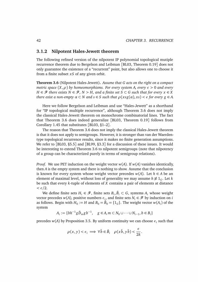
42 CHAPTER 3. RECURRENCE
3.1.2 Nilpotent Hales-Jewett theorem
The following refined version of the nilpotent IP polynomial topological mutiplerecurrence theorem due to Bergelson and Leibman [BL03, Theorem 0.19] does notonly guarantee the existence of a “recurrent” point, but also allows one to choose itfrom a finite subset xS of any given orbit.
Theorem 3.6 (Nilpotent Hales-Jewett). Assume that G acts on the right on a compactmetric space (X ,ρ) by homeomorphisms. For every system A, every ε > 0 and everyH ∈ F there exists N ∈ F , N > H, and a finite set S ⊂ G such that for every x ∈ Xthere exist a non-empty α⊂ N and s ∈ S such that ρ(xsg(α), xs)< ε for every g ∈ A.
Here we follow Bergelson and Leibman and use “Hales-Jewett” as a shorthandfor “IP topological multiple recurrence”, although Theorem 3.6 does not implythe classical Hales-Jewett theorem on monochrome combinatorial lines. The factthat Theorem 3.6 does indeed generalize [BL03, Theorem 0.19] follows fromCorollary 1.45 that substitutes [BL03, §1–2].
The reason that Theorem 3.6 does not imply the classical Hales-Jewett theoremis that it does not apply to semigroups. However, it is stronger than van der Waerden-type topological recurrence results, since it makes no finite generation assumptions.We refer to [BL03, §5.5] and [BL99, §3.3] for a discussion of these issues. It wouldbe interesting to extend Theorem 3.6 to nilpotent semigroups (note that nilpotencyof a group can be characterized purely in terms of semigroup relations).
Proof. We use PET induction on the weight vector w(A). If w(A) vanishes identically,then A is the empty system and there is nothing to show. Assume that the conclusionis known for every system whose weight vector precedes w(A). Let h ∈ A be anelement of maximal level, without loss of generality we may assume h 6≡ 1G . Let kbe such that every k-tuple of elements of X contains a pair of elements at distance< ε/2.
We define finite sets Hi ∈ F , finite sets Bi , Bi ⊂ G, systems Ai whose weightvector precedes w(A), positive numbers εi , and finite sets Ni ∈ F by induction on ias follows. Begin with H0 := H and B0 = B0 = 1G. The weight vector w(Ai) of thesystem
Ai := bh−1 g Dm g b−1, g ∈ A, m⊂ N0 ∪ · · · ∪ Ni−1, b ∈ Bi
precedes w(A) by Proposition 3.5. By uniform continuity we can choose εi such that
ρ(x , y)< εi =⇒ ∀b ∈ Bi ρ(x b, y b)<ε
2k.
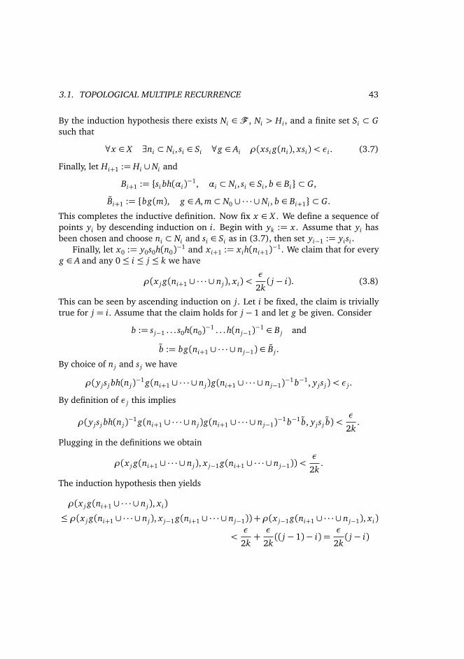
3.1. TOPOLOGICAL MULTIPLE RECURRENCE 43
By the induction hypothesis there exists Ni ∈ F , Ni > Hi , and a finite set Si ⊂ Gsuch that
∀x ∈ X ∃ni ⊂ Ni , si ∈ Si ∀g ∈ Ai ρ(xsi g(ni), xsi)< εi . (3.7)
Finally, let Hi+1 := Hi ∪ Ni and
Bi+1 := si bh(αi)−1, αi ⊂ Ni , si ∈ Si , b ∈ Bi ⊂ G,
Bi+1 := bg(m), g ∈ A, m⊂ N0 ∪ · · · ∪ Ni , b ∈ Bi+1 ⊂ G.
This completes the inductive definition. Now fix x ∈ X . We define a sequence ofpoints yi by descending induction on i. Begin with yk := x . Assume that yi hasbeen chosen and choose ni ⊂ Ni and si ∈ Si as in (3.7), then set yi−1 := yisi .
Finally, let x0 := y0s0h(n0)−1 and x i+1 := x ih(ni+1)−1. We claim that for everyg ∈ A and any 0≤ i ≤ j ≤ k we have
ρ(x j g(ni+1 ∪ · · · ∪ n j), x i)<ε
2k( j− i). (3.8)
This can be seen by ascending induction on j. Let i be fixed, the claim is triviallytrue for j = i. Assume that the claim holds for j− 1 and let g be given. Consider
b := s j−1 . . . s0h(n0)−1 . . . h(n j−1)
−1 ∈ B j and
b := bg(ni+1 ∪ · · · ∪ n j−1) ∈ B j .
By choice of n j and s j we have
ρ(y js j bh(n j)−1 g(ni+1 ∪ · · · ∪ n j)g(ni+1 ∪ · · · ∪ n j−1)
−1 b−1, y js j)< ε j .
By definition of ε j this implies
ρ(y js j bh(n j)−1 g(ni+1 ∪ · · · ∪ n j)g(ni+1 ∪ · · · ∪ n j−1)
−1 b−1 b, y js j b)<ε
2k.
Plugging in the definitions we obtain
ρ(x j g(ni+1 ∪ · · · ∪ n j), x j−1 g(ni+1 ∪ · · · ∪ n j−1))<ε
2k.
The induction hypothesis then yields
ρ(x j g(ni+1 ∪ · · · ∪ n j), x i)
≤ ρ(x j g(ni+1 ∪ · · · ∪ n j), x j−1 g(ni+1 ∪ · · · ∪ n j−1))+ρ(x j−1 g(ni+1 ∪ · · · ∪ n j−1), x i)
<ε
2k+ε
2k(( j− 1)− i) =
ε
2k( j− i)
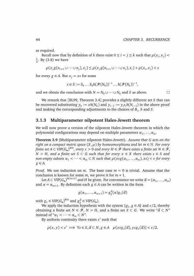
44 CHAPTER 3. RECURRENCE
as required.Recall now that by definition of k there exist 0≤ i < j ≤ k such that ρ(x i , x j)<
ε
2. By (3.8) we have
ρ(x j g(ni+1 ∪ · · · ∪ n j), x j)≤ ρ(x j g(ni+1 ∪ · · · ∪ n j), x i) +ρ(x i , x j)< ε
for every g ∈ A. But x j = xs for some
s ∈ S := Sk . . . S0h(F (N0))−1 . . . h(F (Nk))
−1,
and we obtain the conclusion with N = N0 ∪ · · · ∪ Nk and S as above.
We remark that [BL99, Theorem 3.4] provides a slightly different set S that canbe recovered substituting yk := xh(Nk) and yi−1 := yisih(Ni−1) in the above proofand making the corresponding adjustments to the choices of Bi , b and S.
3.1.3 Multiparameter nilpotent Hales-Jewett theorem
We will now prove a version of the nilpotent Hales-Jewett theorem in which thepolynomial configurations may depend on multiple parameters α1, . . . ,αm.
Theorem 3.9 (Multiparameter nilpotent Hales-Jewett). Assume that G acts on theright on a compact metric space (X ,ρ) by homeomorphisms and let m ∈ N. For everyfinite set A⊂ VIP(G•)
⊗m, every ε > 0 and every H ∈ F there exists a finite set N ∈ F ,N > H, and a finite set S ⊂ G such that for every x ∈ X there exists s ∈ S andnon-empty subsets α1 < · · ·< αm ⊂ N such that ρ(xsg(α1, . . . ,αm), xs)< ε for everyg ∈ A.
Proof. We use induction on m. The base case m = 0 is trivial. Assume that theconclusion is known for some m, we prove it for m+ 1.
Let A⊂ VIP(G•)⊗(m+1) and H be given. For convenience we write ~α = (α1, . . . ,αm)
and α= αm+1. By definition each g ∈ A can be written in the form
g(α1, . . . ,αm+1) = g~α2 (α)g1(~α)
with g1 ∈ VIP(G•)⊗m and g~α2 ∈ VIP(G•).
We apply the induction hypothesis with the system g1, g ∈ A and ε/2, therebyobtaining a finite set N ∈ F , N > H, and a finite set S ⊂ G. We write “~α ⊂ N”instead of “α1 < · · ·< αm ⊂ N”.
By uniform continuity there exists ε′ such that
ρ(x , y)< ε′ =⇒ ∀s ∈ S, ~α⊂ N , g ∈ A ρ(xsg1(~α), ysg1(~α))< ε/2.
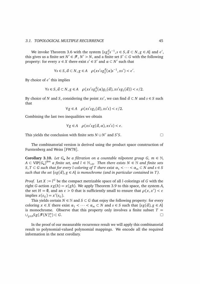
3.1. TOPOLOGICAL MULTIPLE RECURRENCE 45
We invoke Theorem 3.6 with the system sg~α2 s−1, s ∈ S, ~α ⊂ N , g ∈ A and ε′,this gives us a finite set N ′ ∈ F , N ′ > N , and a finite set S′ ⊂ G with the followingproperty: for every x ∈ X there exist s′ ∈ S′ and α⊂ N ′ such that
∀s ∈ S, ~α⊂ N , g ∈ A ρ(xs′sg~α2 (α)s−1, xs′)< ε′.
By choice of ε′ this implies
∀s ∈ S, ~α⊂ N , g ∈ A ρ(xs′sg~α2 (α)g1(~α), xs′sg1(~α))< ε/2.
By choice of N and S, considering the point xs′, we can find ~α⊂ N and s ∈ S suchthat
∀g ∈ A ρ(xs′sg1(~α), xs′s)< ε/2.
Combining the last two inequalities we obtain
∀g ∈ A ρ(xs′sg(~α,α), xs′s)< ε.
This yields the conclusion with finite sets N ∪ N ′ and S′S.
The combinatorial version is derived using the product space construction ofFurstenberg and Weiss [FW78].
Corollary 3.10. Let G• be a filtration on a countable nilpotent group G, m ∈ N,A ⊂ VIP(G•)
⊗m a finite set, and l ∈ N>0. Then there exists N ∈ N and finite setsS, T ⊂ G such that for every l-coloring of T there exist α1 < · · · < αm ⊂ N and s ∈ Ssuch that the set sg(~α), g ∈ A is monochrome (and in particular contained in T).
Proof. Let X := lG be the compact metrizable space of all l-colorings of G with theright G-action x g(h) = x(gh). We apply Theorem 3.9 to this space, the system A,the set H = ;, and an ε > 0 that is sufficiently small to ensure that ρ(x , x ′) < εimplies x(eG) = x ′(eG).
This yields certain N ∈ N and S ⊂ G that enjoy the following property: for everycoloring x ∈ X there exist α1 < · · · < αm ⊂ N and s ∈ S such that sg(~α), g ∈ Ais monochrome. Observe that this property only involves a finite subset T =∪g∈ASg(F (N)m<)⊂ G.
In the proof of our measurable recurrence result we will apply this combinatorialresult to polynomial-valued polynomial mappings. We encode all the requiredinformation in the next corollary.
46 CHAPTER 3. RECURRENCE
Corollary 3.11. Let m ∈ N, K ≤ F ≤ VIP(G•) be VIP groups, and FE≤ VIP(G•)⊗ω be
a countable subgroup that is closed under substitutions g 7→ g[~β] (recall (1.42)).Then for any finite subsets (Ri)ti=0 ⊂ K⊗m∩FE and (Wk)
v−1k=0 ⊂ F⊗m∩FE there exist
N , w ∈ N and (Li , Mi)wi=1 ⊂ (K⊗N ∩ FE)× (F⊗N ∩ FE) such that for every l-coloring
of the latter set there exists an index a and sets β1 < · · · < βm ⊂ N such that theset (LaRi[~β], MaWk[~β]L−1
a )i,k is monochrome (and in particular contained in the set(Li , Mi)wi=1). We may assume L1 ≡ 1G .
Proof. By Proposition 1.41 the maps ~β 7→ (Ri[~β], Wk[~β]Ri[~β]) are polynomialexpressions with values in K⊗ω × F⊗ω. By the assumption they also take valuesin FE × FE. Given an l-coloring χ of (K⊗ω ∩ FE) × (F⊗ω ∩ FE) we pass to thel-coloring χ(g, h) = χ(g, hg−1). Corollary 3.10 then provides the desired N and(Li , Mi)wi=1 = T ∪ S.
3.2 FVIP groups
For reasons that will become clear shortly, our ergodic multiple recurrence resultis restricted to a certain class of VIP systems with the following finite generationproperty.
Definition 3.12. An FVIP group is a finitely generated VIP group. An FVIP system isa member of some FVIP group.
The main result about FVIP groups is the following nilpotent version of [BFM96,Theorem 1.8] and [BHM06, Theorem 1.9] that will be used to construct “primitiveextensions” (we will recall the definitions of a primitive extension and an IP-limit indue time).
Theorem 3.13. Let G• be a prefiltration of finite length and F ≤ VIP(G•) be an FVIPgroup. Suppose that G0 acts on a Hilbert space H by unitary operators and that foreach (gα)α ∈ F the weak limit Pg = w-IP-limα∈F gα exists. Then
1. each Pg is an orthogonal projection and
2. these projections commute pairwise.
The finite generation assumption cannot be omitted in view of a counterexamplein [BFM96].
3.2. FVIP GROUPS 47
3.2.1 Partition theorems for IP-rings
An IP-ring is a subset of F that consists of all finite unions of a given strictlyincreasing chain α0 < α1 < . . . of elements ofF [FK85, Definition 1.1]. In particular,F is itself an IP-ring (associated to the chain 0 < 1 < . . . ). Polynomials aregenerally assumed to be defined on F even if we manipulate them only on somesub-IP-ring of F .
Since we will be dealing a lot with assertions about sub-IP-rings we find itconvenient to introduce a shorthand notation. If some statement holds for a certainsub-IP-ring F ′ ⊂ F then we say that it holds without loss of generality (wlog). Inthis case we reuse the symbol F to denote the sub-IP-ring on which the statementholds (in particular this IP-ring may change from use to use). With this conventionthe basic Ramsey-type theorem about IP-rings reads as follows.
Theorem 3.14 (Hindman [Hin74]). Every finite coloring of F is wlog monochrome.
This is not the same as the assertion “wlog every finite coloring ofF is monochrome”,since the latter would mean that there exists a sub-IP-ring on which every coloring ismonochrome.
As a consequence of Hindman’s theorem 3.14, a map from F to a compactmetric space for every ε > 0 wlog has values in an ε-ball. As the next lemma shows,for polynomial maps into compact metric groups the ball can actually be chosen tobe centered at the identity. In a metric group we denote the distance to the identityby ‖ · ‖.
Lemma 3.15. Let G• be a prefiltration in the category of compact metric groups andP ∈ VIP(G•). Then for every ε > 0 we have wlog ‖P‖< ε.
Proof. We use induction on the length of the prefiltration G•. If the prefiltration istrivial, then there is nothing to show, so assume that the conclusion is known forG•+1.
Let δ,δ′ > 0 be chosen later. By compactness and Hindman’s theorem 3.14 wemay wlog assume that the image P(F ) is contained in some ball B(g,δ) with radiusδ in G1. By uniform continuity of the group operation we have Dβ P(α) ∈ B(g−1,δ′)for any α > β ∈ F provided that δ is small enough depending on δ′. On the otherhand, for a fixed β , by the induction hypothesis we have wlog ‖Dβ P‖< δ′, so that‖g−1‖< 2δ′. By continuity of inversion this implies ‖g‖< ε/2 provided that δ′ issmall enough. This implies ‖P‖< ε provided that δ is small enough.
Corollary 3.16 ([BHM06, Proposition 1.1]). Let W• be a prefiltration, A⊂ VIP(W•)be finite, and V ≤W be a finite index subgroup. Then wlog for every g ∈ A we haveg(F )⊂ V .
48 CHAPTER 3. RECURRENCE
Proof. Let g ∈ A. Passing to a subgroup we may assume that V is normal. Takingthe quotient by V , we may assume that W is finite and V = 1W . By Lemma 3.15with an arbitrary discrete metric we may wlog assume that g ≡ 1W .
In course of proof of Theorem 3.13 it will be more convenient to use a conventionfor the symmetric derivative that differs from (1.37), namely
Dαg(β) = g(α)−1Dαg(β).
Clearly a VIP group is also closed under D.
Lemma 3.17. Let F be a VIP group, W ≤ F be a subgroup and V ≤ W be a finiteindex subgroup. Suppose that g ∈ F is such that the symmetric derivative Dαg ∈W forall α. Then wlog for every α the symmetric derivative Dαg coincides with an element ofV on some sub-IP-ring of the form β ∈ F : β > β0.
Proof. Since V has finite index and by Hindman’s theorem 3.14 we can wlog assumethat Dαg ∈ w−1V for some w ∈W and all α. Assume that w 6∈ V . Let
h(α) := wDαg =
¨
w, α= ;vα ∈ V otherwise.
Let α1 < · · ·< αd be non-empty, by induction on d we see that Dαd. . . Dα1
h(α) ∈ V
for all α 6= ; and Dαd. . . Dα1
h(;) ∈ V w(−1)d V .On the other hand the map α 7→ h(α)(β) is G•+1-polynomial on α : α∩ β = ;
for fixed β . Therefore Dαd. . . Dα1
h(;) vanishes at all β > αd , that is, w coincideswith an element of V on β : β > αd.
It is possible to see Lemma 3.17 (and Lemma 3.53 later on) as a special case ofCorollary 3.16 by considering the quotient of VIP(G•) by the equivalence relation ofequality on IP-rings of the form α : α > α0, but we prefer not to set up additionalmachinery.
In order to apply the above results we need a tool that provides us with finite in-dex subgroups. To this end recall the following multiparameter version of Hindman’stheorem 3.14.
Theorem 3.18 (Milliken [Mil75], Taylor [Tay76]). Every finite coloring of F k< is
wlog monochrome.
The next lemma is a substitute for [BFM96, Lemma 1.6] in the non-commutativecase. This is the place where the concept of Hirsch length is utilized.
3.2. FVIP GROUPS 49
Lemma 3.19. Let G be a finitely generated nilpotent group and g : F → G be anymap. Then wlog there exist a natural number l > 0 and a subgroup W ≤ G such thatfor any α1 < · · ·< αl ∈ F the elements gα1
, . . . , gαlgenerate a finite index subgroup
of W.
Proof. By the Milliken-Taylor theorem 3.18 we may wlog assume that for eachl ≤ h(G) + 1 the Hirsch length h(
¬
gα1, . . . , gαl
¶
) does not depend on (α1, . . . ,αl) ∈F l<. Call this value hl . It is an increasing function of l that is bounded by h(G),
hence there exists an l such that hl = hl+1. Fix some (α1, . . . ,αl) ∈ F l< and let
V :=¬
gα1, . . . , gαl
¶
.Since hl+1 = hl and by Lemma 1.17, we see that
V, gα
is a finite indexextension of V for each α > αl . By Corollary 1.19 and Hindman’s Theorem 3.14we may wlog assume that each gα lies in one such extension W . By definitionof hl this implies that wlog for every (α1, . . . ,αl) ∈ F l
< the Hirsch length of thegroup
¬
gα1, . . . , gαl
¶
≤W is h(W ). Hence each¬
gα1, . . . , gαl
¶
≤W is a finite indexsubgroup by Lemma 1.17.
3.2.2 IP-limits
Let X be a topological space, m ∈ N and g :Fm< → X be a map. We call x ∈ X an
IP-limit of g, in symbols IP-lim~α g~α = x , if for every neighborhood U of x there existsα0 such that for all ~α ∈ Fm
< , ~α > α0, one has g~α ∈ U .By the Milliken-Taylor theorem 3.18 and a diagonal argument, cf. [FK85, Lemma
1.4], we may wlog assume the existence of an IP-limit (even of countably manyIP-limits) if X is a compact metric space, see [FK85, Theorem 1.5].
If X is a Hilbert space with the weak topology, then we write w-IP-lim instead ofIP-lim to stress the topology.
Following a tradition, we write arguments of maps defined on F as subscriptsin this section. We also use the notation and assumptions of Theorem 3.13.
The next lemma follows from the equivalence of the weak and the strongtopology on the unit sphere of H and is stated for convenience.
Lemma 3.20. Assume that f ∈ fix Pg , that is, that w-IP-limα gα f = f . Then alsoIP-limα gα f = f (in norm).
For any subgroup V ≤ F we write PV for the orthogonal projection onto thespace
⋂
g∈V fix Pg .
Lemma 3.21. Assume that V =
g1, . . . , gs
is a finitely generated group and thatPg1
, . . . , Pgsare commuting projections. Then PV =
∏si=1 Pgi
.
50 CHAPTER 3. RECURRENCE
Proof. Clearly we have PV ≤∏s
i=1 Pgi, so we only need to prove that each f that is
fixed by Pg1, . . . , Pgs
is also fixed by Pg for any other g ∈ V .To this end it suffices to show that if f is fixed by Pg and Ph for some g, h ∈
V , then it is also fixed by Pgh−1 . Lemma 3.20 shows that IP-limα gα f = f andIP-limα hα f = f . Since each hα is unitary we obtain IP-limα h−1
α f = f . Since eachgα is isometric, this implies
w-IP-lim gαh−1α f = IP-lim
αgαh−1
α f = f
as required.
The next lemma is the main tool to ensure IP-convergence to zero.
Lemma 3.22 ([BFM96, Lemma 1.7]). Let (Pα)α∈F be a family of commuting orthogo-nal projections on a Hilbert space H and f ∈ H. Suppose that, whenever α1 < · · ·< αl ,one has
∏li=1 Pαi
f = 0. Then IP-limα ‖Pα f ‖= 0.
Finally, we also need a van der Corput-type estimate.
Lemma 3.23 ([FK85, Lemma 5.3]). Let (xα)α∈F be a bounded family in a Hilbertspace H. Suppose that
IP-limβ
IP-limα
¬
xα, xα∪β¶
= 0.
Then wlog we havew-IP-lim
αxα = 0.
Proof of Theorem 3.13. We proceed by induction on the length of the prefiltrationG•. If G• is trivial there is nothing to prove. Assume that the conclusion is knownfor G•+1.
First, we prove that Pg is an orthogonal projection for any g ∈ F (that we nowfix). Since Pg is clearly contractive it suffices to show that it is a projection.
By Lemma 3.19 we may assume that, for some l > 0 and any α1 < · · ·< αl , thederivatives Dα1
g, . . . , Dαlg generate a finite index subgroup of some W ≤ F1 (recall
that F1 = F ∩ VIP(G•+1)). We split
H =⋂
V≤W
ker PV ⊕ lin⋃
V≤W
im PV
=: H0 ∪H1, (3.24)
where V runs over the finite index subgroups of W . It suffices to show Pg f = P2g f
for each f in one of these subspaces.
3.2. FVIP GROUPS 51
Case 0 Let f ∈ H0 and α1 < · · ·< αl . By choice of W we know that
V :=¬
Dα1g, . . . , Dαl
g¶
≤W
is a finite index subgroup. Since the projections PDαig commute by the inductive
hypothesis, their product equals PV (Lemma 3.21), and we have PV f = 0 by theassumption.
By Lemma 3.22 this implies IP-limα ‖PDα g f ‖= 0. Therefore
IP-limα
IP-limβ
¬
(Dαg)β f , g−1α f¶
≤ IP-limα‖w-IP-lim
β(Dαg)β f ‖
= IP-limα‖PDα g f ‖= 0,
so thatIP-limα
IP-limβ
¬
gα∪β f , gβ f¶
= 0.
By Lemma 3.23 this implies Pg f = 0 (initially only wlog, but we have assumed thatthe limit exists on the original IP-ring).
Case 1 Let V ≤W and f = PV f , by linearity we may assume ‖ f ‖ = 1. Let ρ bea metric for the weak topology on the unit ball of H with ρ(x , y) ≤ ‖x − y‖. Letε > 0. By definition of IP-convergence and by uniform continuity of Pg there existsα0 such that
∀α > α0 ρ(gα f , Pg f )< ε and ρ(Pg gα f , P2g f )< ε.
By Lemma 3.17 we can choose α > α0 such that Dαg coincides with an element ofV on some sub-IP-ring, so that in particular PDα g f = f . By Lemma 3.20 there existsβ0 > α such that
∀β > β0 ‖(Dαg)β f − f ‖< ε.
Applying gβ gα to the difference on the left-hand side we obtain
‖gα∪β f − gβ gα f ‖< ε, so that ρ(gα∪β f , gβ gα f )< ε.
Observe that α∪ β > α0, so that
ρ(Pg f , gβ gα f )< 2ε.
Taking IP-limit along β we obtain
ρ(Pg f , Pg gα f )≤ 2ε.
52 CHAPTER 3. RECURRENCE
A further application of the triangle inequality gives
ρ(Pg f , P2g f )< 3ε,
and, since ε > 0 was arbitrary, we obtain Pg f = P2g f .
Commutativity of projections Let us now prove the second conclusion, namelythat Pg and Pg ′ commute for any g, g ′ ∈ F . Observe that the function α 7→ gα can beseen as a polynomial-valued function in VIP(P(G , G•)) whose values are constantpolynomials. Moreover we can consider the constant function in P(G , F•) whosevalue is g ′. Taking their commutator we see that
α 7→ [gα, g ′] ∈ VIP(P(G , G•)),
and, since F is a VIP group, this map in fact lies in VIP(F•). By (1.36) it takesvalues in F1. By Lemma 3.19 we may assume that for any α1 < · · · < αl themaps [gα1
, g ′], . . . , [gαl, g ′] generate a finite index subgroup of some W ≤ F1.
Interchanging g and g ′ and repeating this argument we may also wlog assumethat for any α1 < · · · < αl ′ the maps [g ′α1
, g], . . . , [g ′αl′, g] generate a finite index
subgroup of some W ′ ≤ F1. Consider the splitting
H =⋂
V≤W
ker PV∩⋂
V ′≤W ′
ker PV ′
⊕lin⋃
V≤W
im PV∪⋃
V ′≤W ′
im PV ′
=: H0∪H1. (3.25)
Case 0 Let f ∈ H0. As above we have IP-limα ‖P[gα,g ′] f ‖= 0, and in particular
0= IP-limα
w-IP-limβ
[gα, g ′β] f , g−1α Pg ′ f
= IP-limα
IP-limβ
D
gαg ′β f , g ′β Pg ′ fE
= IP-limα
¬
gαPg ′ f , Pg ′ f¶
,
since IP-limβ g ′β Pg ′ f = Pg ′ f by Lemma 3.20. Hence Pg Pg ′ f ⊥ Pg ′ f , which impliesPg Pg ′ f = 0 since Pg is an orthogonal projection.
Interchanging the roles of g and g ′, we also obtain Pg ′Pg f = 0.
Case 1 Let V ≤ W and f = PV f . By Corollary 3.16 we may wlog assume that[gα, g ′] ∈ V for all α. Let α be arbitrary, by Lemma 3.20 the limit
IP-limβ[gα, g ′β] f = f
3.2. FVIP GROUPS 53
also exists in norm. Therefore
gαPg ′ f = w-IP-limβ
gαg ′β f = w-IP-limβ
g ′β gα[gα, g ′β] f = w-IP-limβ
g ′β gα f = Pg ′ gα f .
Taking IP-limits on both sides we obtain
Pg Pg ′ f = Pg ′Pg f .
The case V ′ ≤W ′ and f = PV ′ f can be handled in the same way.
If the group G acts by measure-preserving transformations then the Hilbert spaceprojections identified in Theorem 3.13 are in fact conditional expectations as thefollowing folklore lemma shows.
Lemma 3.26. Let X be a probability space and (Tα)α be a net of operators on L2(X )induced by measure-preserving transformations. Assume that Tα→ P weakly for someprojection P. Then P is a conditional expectation.
Proof. Note that im P ∩ L∞(X ) is dense in im P.Let f , g ∈ im P ∩ L∞(X ). Since the weak and the norm topology coincide on the
unit sphere of L2(X ), we have ‖Tα f − f ‖2→ 0 and ‖Tαg − g‖2→ 0. Therefore
‖P( f g)− f g‖2 ≤ limsupα‖Tα( f g)− f g‖2
= limsupα‖(Tα f − f )Tαg + f (Tαg − g)‖2
≤ limsupα‖Tα f − f ‖2‖Tαg‖∞ + ‖ f ‖∞‖Tαg − g‖2 = 0.
This shows that im P ∩ L∞(X ) is an algebra, and the assertion follows.
3.2.3 Generalized polynomials and FVIP groups
In order to obtain some tangible combinatorial applications of our results we willneed non-trivial examples of FVIP groups. The first example somewhat parallelsProposition 1.43.
Lemma 3.27 ([BHM06]). Let (n1i )i∈N, . . . , (na
i )i∈N ⊂ Z be any sequences, (G,+) be acommutative group, (yi)i∈N ⊂ G be any sequence, and d ∈ N. Then the maps of theform
v(α) =∑
i1<···<ie∈αn j1
i1· · ·n je−1
ie−1yie , e ≤ d, 1≤ j1, . . . , je−1 ≤ a, (3.28)
54 CHAPTER 3. RECURRENCE
generate an FVIP subgroup F ≤ VIP(G•), where the prefiltration G• is given by G0 =· · ·= Gd = G, Gd+1 = 1G.
Maps of the form (3.28) were originally studied in connection with admissiblegeneralized polynomials (Definition 3.31). We will not return to them in the sequeland a proof of the above lemma is included for completeness.
Proof. The group F is by definition finitely generated and closed under conjugationby constants since G is commutative. It remains to check that the maps of the form(3.28) are polynomial and that the group F is closed under symmetric derivatives.
To this end we use induction on d. The cases d = 0,1 are clear (in the lattercase the maps (3.28) are IP-systems), so let d > 1 and consider a map v as in (3.28)with e = d. For β < α we have
Dβ v(α) =−v(α) + v(β ∪α)− v(β)
=d−1∑
k=1
∑
i1<···<ik∈β ,ik+1<···<id∈α
n j1i1· · ·n je−1
id−1yid
=d−1∑
k=1
∑
i1<···<ik∈β
n j1i1· · ·n jk
ik
∑
ik+1<···<id∈αn jk+1
ik+1· · ·n je−1
id−1yid .
The underlined expression is G•+1-polynomial by the induction hypothesis and liesin F by definition. Since this holds for every β , the map v is G•-polynomial. Sincethe derivatives are in F for every map v, the group F is FVIP.
The following basic property of FVIP groups will be used repeatedly.
Lemma 3.29. Let F, F ′ ≤ VIP(G•) be FVIP groups. Then the group F ∨ F ′ is also FVIP.
Proof. The group F ∨ F ′ is clearly finitely generated and invariant under conjugationby constants. Closedness under D follows from the identity
Dm(gh) = h−1 Dm g g(m)hDmhg(m)−1. (3.30)
We will now elaborate on the example that motivated Bergelson, Håland Knutsonand McCutcheon to study FVIP systems in the first place [BHM06]. They have shownthat ranges of generalized polynomials from a certain class necessarily contain FVIPsystems.
We begin by recalling the definition of the appropriate class. We denote theinteger part function by b·c, the nearest integer function by b·e= b·+ 1/2c and the
3.2. FVIP GROUPS 55
distance to nearest integer by ‖a‖= |a− bae| (this is consistent with the notationfor general metric groups applied to R/Z).
Definition 3.31. The set G of generalized polynomials (in l variables) is the small-est Z-algebra of functions Zl → Z that contains Z[x1, . . . , x l] such that for everyp1, . . . , pt ∈ G and c1, . . . , ct ∈ R the map b
∑ti=1 ci pic is in G . The notion of degree is
extended from Z[x1, . . . , x l] to G inductively by requiring deg p0p1 ≤ deg p0+deg p1,deg(p0 + p1) ≤ max(deg p0, deg p1), and degb
∑ti=1 ci pic ≤ maxi deg pi , the degree
of each generalized polynomial being the largest number with these properties.The set of Ga of admissible generalized polynomials is the smallest ideal of G that
contains the maps x1, . . . , x l and is such that for every p1, . . . , pt ∈ Ga, c1, . . . , ct ∈ R,and 0< k < 1 the map b
∑ti=1 ci pi + kc is in Ga.
Some examples of generalized polynomials are
n3 + n, [πn+ 1/2], [πn+ 1/2][πn], [πn2[en] + 1/e],
[p
2n3 + 1/e][log 3 · [p
3n2 + n]2 + n], n5 − n+ 1, [πn], (3.32)
of which all but the last two are admissible.The construction of FVIP systems in the range of an admissible generalized
polynomial in [BHM06] proceeds by induction on the polynomial and utilizesLemma 3.27 at the end. We give a softer argument that gives a weaker result inthe sense that it does not necessarily yield an FVIP system of the form (3.28), butrequires less computation.
For a ring R (with not necessarily commutative multiplication, although we willonly consider R = Z and R = R in the sequel) and d ∈ N we denote by Rd
• theprefiltration (with respect to the additive group structure) given by R0 = · · · = Rd =R and Rd+1 = 0R.
Lemma 3.33. Let Fi ≤ VIP(Rdi• ), i = 0, 1, be FVIP groups. Then the pointwise products
of maps from F0 and F1 generate an FVIP subgroup of VIP(Rd0+d1• ).
Proof. This follows by induction on d0 + d1 using the identity
Dβ vw = (v+ Dβ v+ v(β))Dβw+ (Dβ v + v(β))w+ (Dβ v + v)w(β)
for the symmetric derivative of a pointwise product.
Applying Lemma 3.15 to R/Z we obtain the following.
Corollary 3.34. Let P be an FVIP system in R. Then for every ε > 0 wlog ‖P‖< ε.
56 CHAPTER 3. RECURRENCE
This allows us to show that we can obtain Z-valued FVIP systems from R-valuedFVIP-systems by rounding.
Lemma 3.35. Let P ∈ VIP(Rd• ) be an FVIP system. Then wlog bPe ∈ VIP(Zd
• ) and bPeis an FVIP system.
Proof. We use induction on d. For d = 0 there is nothing to show, so assumethat d > 0. By the assumption every symmetric derivative of (Pα) lies in an FVIPgroup of polynomials of degree < d that is generated by q1, . . . , qa, say. By theinduction hypothesis we know that wlog each bqie is again an FVIP system and byLemma 3.29 they lie in some FVIP group F . By Corollary 3.34 we may assume wlogthat ‖P‖< 1/12. Let now β be given, by the hypothesis we have
Dβ P(α) =∑
i
ciqi(α) for α > β
with some ci ∈ Z. By Corollary 3.34 we may wlog assume that |ci |·‖qi‖(α)< 1/(4·2i)for all α > β . This implies
|DβbPe(α)−∑
i
cibqie(α)|< 1/2 for α > β ,
so thatDβbPe(α) =
∑
i
cibqie(α) for α > β ,
since both sides are integer-values functions. In fact we can do this for all β withfixed maxβ simultaneously. By a diagonal argument, cf. [FK85, Lemma 1.4], wemay then assume that for every β we have
DβbPe(α) =∑
i
cibqie(α) for α > β
with some ci ∈ Z. Hence F ∨ ⟨bPe⟩ ≤ VIP(Zd• ) is an FVIP group.
Recall that an IP-system in Zl is a family (nα)α∈F ⊂ Zl such that nα∪β = nα + nβwhenever α,β ∈ F are disjoint.
Theorem 3.36 ([BHM06, Theorem 2.8]). For every generalized polynomial p : Zl →Z and every FVIP system (nα)α in Zl of degree at most d there exists n ∈ Z such that theIP-sequence (p(nα)− n)α∈F is wlog FVIP of degree at most d deg p. If p is admissible,then we may assume n= 0.
3.2. FVIP GROUPS 57
For inadmissible polynomials it may not be possible to obtain the above resultwith n= 0. Indeed, consider the example p(n) = [πn]. Since πn is equidistributedmodulo 2, we can find a sequence (nk) such that πnk ∈ (−2−k, 0) mod 2 for eachk. Consider the IP system nα =
∑
k∈α nk. Then πnα ∈ (−1,0) mod 2 for eachα ∈ F , so that p(nα) is odd. Lemma 3.15 applied to Z/2Z now shows that nosub-IP-sequence of (p(nα))α∈F can be a VIP system.
Proof. We begin with the first part and use induction on p. The class of maps thatsatisfy the conclusion is closed under Z-linear combinations by Lemma 3.29 andunder multiplication by Lemma 3.33. This class clearly contains the polynomials1, x1, . . . , x l . Thus it remains to show that, whenever p1, . . . , pt ∈ G satisfy theconclusion and c1, . . . , ct ∈ R, the map bPc with P =
∑ti=1 ci pi also satisfies the
conclusion.By the assumption we have wlog that (P(nα)− C)α is an R-valued FVIP system
for some C ∈ R. By Hindman’s theorem 3.14 we may wlog assume that bP(nα)c=bP(nα)− Ce+ n for some integer n with |n− C |< 2 and all α ∈ F . The conclusionfollows from Lemma 3.35.
Now we consider admissible generalized polynomials p and use induction on pagain. The conclusion clearly holds for x1, . . . , x l , passes to linear combinations andpasses to products with arbitrary generalized polynomials by Lemma 3.33 and thefirst part of the statement. Assume now that p1, . . . , pt ∈ Ga satisfy the conclusionand c1, . . . , ct ∈ R, 0 < k < 1. Then (P(nα))α with P :=
∑ti=1 ci pi is wlog an R-
valued FVIP system, and by Corollary 3.34 we have wlog ‖P‖<min(k, 1− k). Thisimplies bP(nα) + kc = bP(nα)e and this is wlog an FVIP system by Lemma 3.35.
As an aside, consider the set of real-valued generalized polynomials RG [BM10,Definition 3.1] that is defined similarly to G , except that it is required to be anR-algebra. Following the proof of Theorem 3.36 we see that for every p ∈ RGand every FVIP system (nα)α ⊂ Zl wlog there exists a constant C ∈ R such that(p(nα)− C)α is an FVIP system. Clearly, if p is of the form bqc then C ∈ Z andif p ∈ R[x1, . . . , x l] with zero constant term then C = 0. This, together withCorollary 3.34, implies (an FVIP* version of) [BL07, Theorem D].
Our main example (that also leads to Theorem 3.1) are maps induced by admis-sible generalized polynomial sequences in finitely generated nilpotent groups.
Lemma 3.37. Let G be a finitely generated nilpotent group with a filtration G•. Letp : Zl → Z be an admissible generalized polynomial, (nα)α ⊂ Zl be an FVIP system ofdegree at most d and g ∈ Gd deg p. Then wlog (g p(nα))α is an element of VIP(G•) andan FVIP system.
58 CHAPTER 3. RECURRENCE
Proof. By Theorem 3.36 we can wlog assume that (p(nα))α is a Z-valued FVIP systemof degree ≤ d deg p. Using the (family of) homomorphism(s) Zd deg p
• → G•, 1 7→ g,we see that (g p(nα))α is contained in a finitely generated subgroup F0 ≤ VIP(G•) thatis closed under D.
Let A⊂ F0 and B ⊂ G be finite generating sets. Then the group generated bybab−1, a ∈ A, b ∈ B, is FVIP in view of the identity (3.30).
3.3 Measurable multiple recurrence
Following the general scheme of Furstenberg’s proof, we will obtain our multiplerecurrence theorem by (in general transfinite) induction on a suitable chain offactors of the given measure-preserving system. For the whole section we fix anilpotent group G with a filtration G• and an FVIP group F ≤ VIP(G•).
In the induction step we pass from a factor to a “primitive extension” that enjoysa dichotomy: each element of F acts on it either relatively compactly or relativelymixingly. Since the reasoning largely parallels the commutative case here, we areable to refer to the article of Bergelson and McCutcheon [BM00] for many proofs.The parts of the argument that do require substantial changes are given in full detail.
Whenever we talk about measure spaces (X ,A ,µ), (Y,B ,ν), or (Z ,C ,γ) wesuppose that they are regular and that G acts on them on the right by measure-preserving transformations. This induces a left action on the corresponding L2
spaces. Recall that to every factor map (Z ,C ,γ)→ (Y,B ,ν) there is associated anessentially unique measure disintegration
γ=
∫
y∈Y
γydν(y),
see [Fur81, §5.4]. We write ‖ · ‖y for the norm on L2(Z ,γy). Recall also that thefiber product Z ×Y Z is the space Z × Z with the measure
∫
y∈Yγy ⊗ γydν(y).
3.3.1 Compact extensions
We begin with the appropriate notion of relative compactness. Heuristically, anextension is relatively compact if it is generated by the image of a relatively Hilbert-Schmidt operator.
Definition 3.38 ([BM00, Definition 3.4]). Let Z → Y be a factor. A Z |Y -kernel is a
3.3. MEASURABLE MULTIPLE RECURRENCE 59
function H ∈ L∞(Z ×Y Z) such that∫
H(z1, z2)dγz2(z1) = 0
for a.e. z2 ∈ Z . If H is a Z |Y -kernel and φ ∈ L2(Z) then
H ∗φ(z1) :=
∫
H(z1, z2)φ(z2)dγz1(z2).
The map φ 7→ H ∗φ is a Hilbert-Schmidt operator on almost every fiber overY with uniformly bounded Hilbert-Schmidt norm. These operators are self-adjointprovided that H(z1, z2) = H(z2, z1) a.e.
Definition 3.39 ([BM00, Definition 3.6]). Suppose that X → Z → Y is a chain offactors, K ≤ F is a subgroup and H is a non-trivial self-adjoint X |Y -kernel that isK-invariant in the sense that
IP-limα
g(α)H = H
for every g ∈ K. The extension Z → Y is called K-compact if it is generated byfunctions of the form H ∗φ, φ ∈ L2(X ).
Lemma 3.40 ([BM00, Remark 3.7(i)]). Let X → Z → Y be a chain of factors inwhich Z → Y is a K-compact extension generated by a X |Y -kernel H. Then H is in facta Z |Y -kernel and Z is generated by functions of the form H ∗φ, φ ∈ L2(Z).
Proof. Call the projection maps π : X → Z , θ : X → Y . Let φ ∈ L2(X ). Since H ∗φis Z-measurable we have
H ∗φ(x) =∫
H ∗φ(x1)dµπ(x)(x1)
=
∫ ∫
H(x1, x2)φ(w2)dµθ(x1)(x2)dµπ(x)(x1)
=
∫ ∫
H(x1, x2)φ(x2)dµθ(x)(x2)dµπ(x)(x1)
=
∫ ∫
H(x1, x2)dµπ(x)(x1)φ(x2)dµθ(x)(x2)
= E(H|Z ×Y X ) ∗φ(w).
60 CHAPTER 3. RECURRENCE
Since this holds for all φ we obtain H = E(H|Z ×Y X ). Since H is self-adjoint thisimplies that H is Z ×Y Z-measurable. This in turn implies that H ∗φ = H ∗E(φ|Z)for all φ ∈ L2(X ).
In view of this lemma the reference to the ambient space X is not necessary in thedefinition of a K-compact extension. Just like in the commutative case, compactnessis preserved upon taking fiber products (this is only used in the part of the proof ofTheorem 3.55 that we do not write out).
Lemma 3.41 ([BM00, Remark 3.7(ii)]). Let Z → Y be a K-compact extension. ThenZ ×Y Z → Y is also a K-compact extension.
3.3.2 Mixing and primitive extensions
Now we define what we mean by relative mixing and the dichotomy betweenrelative compactness and relative mixing.
Definition 3.42 ([BM00, Definition 3.5]). Let Z → Y be an extension. A map g ∈ Fis called mixing on Z relatively to Y if for every H ∈ L2(Z ×Y Z) with E(H|Y ) = 0one has w-IP-limα g(α)H = 0. An extension Z → Y is called K-primitive if it isK-compact and each g ∈ F \ K is mixing on Z relative to Y .
The above notion of mixing might be more appropriately called “mild mixing”,but we choose a shorter name since there will be no danger of confusion.
The next lemma is used in the suppressed part of the proof of Theorem 3.55.
Lemma 3.43 ([BM00, Proposition 3.8]). Let Z → Y be a K-primitive extension.Then Z ×Y Z → Y is also a K-primitive extension.
Like in the commutative setting [McC05, Lemma 2.8] the compact part of aprimitive extension is wlog closed under taking derivatives, but there is also a newaspect, namely that it is also closed under conjugation by constants.
Lemma 3.44. Let Z → Y be a K-primitive extension. Then K is closed under conjuga-tion by constant functions. Moreover wlog K is an FVIP group.
Proof. Let g ∈ F \ K , h ∈ G and H ∈ L2(Z ×Y Z) be such that E(H|Y ) = 0. Then
w-IP-limα
(h−1 gh)(α)H = h−1 w-IP-limα
g(α)(hH) = 0,
so that F \ K is closed under conjugation by constant functions, so that K is alsoclosed under conjugation by constant functions.
3.3. MEASURABLE MULTIPLE RECURRENCE 61
Since F is Noetherian, the subgroup K is finitely generated as a semigroup. Fixa finite set of generators for K . By Hindman’s Theorem 3.14 we may wlog assumethat for every generator g we have either Dαg ∈ K for all α ∈ F or Dαg 6∈ K for allα ∈ F . In the latter case we obtain
0= w-IP-limα,β
Dβ g(α)H = IP-limα,β
g(α)−1 g(α∪ β)g(β)−1H = H,
a contradiction. Thus we may assume that all derivatives of the generators lie in K .This extends to the whole group K by (3.30) and invariance of K under conjugationby constants.
3.3.3 Existence of primitive extensions
Since our proof proceeds by induction over primitive extensions we need to knowthat such extensions exist. First, we need a tool to locate non-trivial kernels.
Lemma 3.45 ([BM00, Lemma 3.12]). Let X → Y be an extension. Suppose that0 6= H ∈ L2(X ×Y X ) satisfies E(H|Y ) = 0 and that there exists g ∈ F such thatIP-limα g(α)H = H.
Then there exists a non-trivial self-adjoint non-negative definite X |Y -kernel H ′ suchthat IP-limα g(α)H ′ = H ′.
Second, we have to make sure that we cannot accidentally trivialize them.
Lemma 3.46 ([BM00, Lemma 3.14]). Let Z → Y be a K-compact extension. Supposethat for some g ∈ K and self-adjoint non-negative definite Z |Y -kernel H we have
IP-limα
∫
(g(α)H)( f ′ ⊗ f ′)dγ= 0
for all f ′ ∈ L∞(Z). Then H = 0.
The next theorem that provides existence of primitive extensions can be provedin the same way as in the commutative case [BM00, Theorem 3.15]. The onlychange is that Theorem 3.13 is used instead of [BM00, Theorem 2.17] (note that Fis Noetherian, since it is a finitely generated nilpotent group).
Theorem 3.47. Let X → Y be a proper factor. Then there exists a subgroup K ≤ F anda factor X → Z → Y such that the extension Z → Y is proper and wlog K-primitive.
62 CHAPTER 3. RECURRENCE
3.3.4 Almost periodic functions
For the rest of Section 3.3 we fix a good group FE ≤ VIP(G•)⊗ω. We will describe
what we mean by “good” in Definition 3.60, for the moment it suffices to say thatFE is countable.
Definition 3.48 ([BM00, Definition 3.1]). Suppose that (Z ,C ,γ)→ (Y,B ,ν) is afactor and K ≤ F a subgroup. A function f ∈ L2(Z) is called K-almost periodic iffor every ε > 0 there exist g1, . . . , gl ∈ L2(Z) and D ∈ B with ν(D) < ε such thatfor every δ > 0 and R ∈ K⊗ω ∩ FE there exists α0 such that for every α0 < ~α ∈ Fω
<
there exists a set E = E(~α) ∈B with ν(E)< δ such that for all y ∈ Y \ (D∪ E) thereexists 1≤ j ≤ l such that
‖R(α) f − g j‖y < ε.
The set of K-almost periodic functions is denoted by AP(Z , Y, K).
The next lemma says that a characteristic function that can be approximated byalmost periodic functions can be replaced by an almost periodic function right away.
Lemma 3.49 ([BM00, Theorem 3.3]). Let A∈ C be such that 1A ∈ AP(Z , Y, K) andδ > 0. Then there exists a set A′ ⊂ A such that γ(A\ A′)< δ and 1A′ ∈ AP(Z , Y, K).
In the following lemma we have to restrict ourselves to K⊗ω ∩ FE since K⊗ω
need not be countable.
Lemma 3.50 ([BM00, Proposition 3.9]). Let X → Y be an extension, K ≤ F asubgroup and H a X |Y -kernel that is K-invariant. Then wlog for all R ∈ K⊗ω ∩FE andε > 0 there exists α0 such that for all α0 < ~α we have
‖R(~α)H −H‖< ε.
With help of the above lemma we can show that in fact wlog every characteristicfunction can be approximated by almost periodic functions. In view of Lemma 3.49this allows us to reduce the question of multiple recurrence in a primitive extensionto multiple recurrence for (relatively) almost periodic functions.
Lemma 3.51 ([BM00, Theorem 3.11]). Let Z → Y be a K-compact extension. Thenwlog AP(Z , Y, K) is dense in L2(Z).
3.3.5 Multiple mixing
Under sufficiently strong relative mixing assumptions the limit behavior of a mul-ticorrelation sequence
∏
i Si(α) fi on a primitive extension only depends on the
3.3. MEASURABLE MULTIPLE RECURRENCE 63
expectations of the functions on the base space. The appropriate conditions on theset Sii are as follows.
Definition 3.52. Let K ≤ F be a subgroup. A subset A ⊂ F is called K-mixing if1G ∈ A and g−1h ∈ F \ K whenever g 6= h ∈ A.
The requirement 1G ∈ A is not essential, but it is convenient in inductive argu-ments. In order to apply PET induction we will need the next lemma.
We say that a subgroup K ≤ F is invariant under equality of tails if wheneverS ∈ K and T ∈ F are such that there exists β ∈ F with Sα = Tα for all α > β wehave T ∈ K . Every group K ≤ F that is the compact part of some primitive extensionhas this property.
Lemma 3.53. Let K ≤ F be a subgroup that is invariant under equality of tails. LetS, T ∈ F be such that S−1T 6∈ K. Then wlog
(SDβS)−1(T DβT ) 6∈ K and S−1(T DβT ) 6∈ K
for all β ∈ F .
Proof. If the first conclusion fails then by Hindman’s theorem 3.14 wlog
h(α) := (SDαS)−1(T DαT ) ∈ K for all α ∈ F
and h(;) 6∈ K . Proceed as in the proof of Lemma 3.17. Analogously for the secondconclusion.
The next lemma is a manifestation of the principle that compact orbits can bethought of as being constant.
Lemma 3.54 ([BM00, Proposition 4.2]). Let Z → Y be a K-primitive extension,Rβ ∈ K for each β ∈ F and W ∈ F \ K. Let also f , f ′ ∈ L∞(Z) be such that eitherE( f |Y ) = 0 or E( f ′|Y ) = 0. Then wlog
IP-limβ ,α‖E(Rβ(α) f W (β) f ′|Y )‖= 0.
We come to the central result on multiple mixing.
Theorem 3.55 (cf. [BM00, Theorem 4.10]). Let K ≤ F be a subgroup. For everyK-mixing set S0 ≡ 1G , S1, . . . , St ⊂ F the following statements hold.
64 CHAPTER 3. RECURRENCE
1. For every K-primitive extension Z → Y and any f0, . . . , ft ∈ L∞(Z) we have wlog
w-IP-limα
t∏
i=1
Si(α) fi −t∏
i=1
Si(α)E( fi |Y ) = 0.
2. For every K-primitive extension Z → Y and any f0, . . . , ft ∈ L∞(Z) we have wlog
IP-limα
E
t∏
i=0
Si(α) fi
Y
−t∏
i=0
Si(α)E( fi |Y )
= 0.
3. For every K-primitive extension Z → Y , any Ui, j ∈ K, and any fi, j ∈ L∞(Z) wehave wlog
IP-limα
E
t∏
i=0
Si(α)
s∏
j=0
Ui, j(α) fi, j
Y
−t∏
i=0
Si(α)E
s∏
j=0
Ui, j(α) fi, j
Y
= 0.
We point out that the main induction loop is on the mixing set. It is essential that,given K ≤ F , all statements are proved simultaneously for all K-compact extensionssince the step from weak convergence to strong convergence involves a fiber productvia Lemma 3.43.
Proof. The proof is by PET-induction on the mixing set. We only prove that the laststatement for mixing sets with lower weight vector implies the first, the proofs ofother implications are the same as in the commutative case.
By the telescope identity it suffices to consider the case E( fi0 |Y ) = 0 for some i0.By the van der Corput Lemma 3.23 it suffices to show that wlog
IP-limβ ,α
∫
Z
t∏
i=1
Si(α) fi
t∏
i=1
Si(α∪ β) fi = 0.
This limit can be written as
IP-limβ ,α
∫
Z
t∏
i=1
Si(α) fi
t∏
i=1
Si(α)DβSi(α)︸ ︷︷ ︸
=:Ti,β (α)
(Si(β) fi).
By Lemma 3.53 we may wlog assume that T−1i,β T j,β and S−1
i T j,β are mixing forall β ∈ F provided that i 6= j. Re-indexing if necessary and using Hindman’s
3.3. MEASURABLE MULTIPLE RECURRENCE 65
theorem 3.14 we may wlog assume S−1i Ti,β ∈ K for all β ∈ F and i ≤ w and
S−1i Ti,β 6∈ K for all β ∈ F and i > w for some w = 0, . . . , t. Thus
S0, S1, . . . , St , Tw+1,β , . . . , Tt,β (3.56)
is a K-mixing set for every β 6= ;. Moreover it has the same weight vector asS1, . . . , St since Ti,β ∼ Si . Assume that S j , j 6= 0, has the maximal level in (3.56).We have to show
IP-limβ ,α
∫
Z
w∏
i=1
S−1j (α)Si(α)( fi DβSi(α)(Si(β) fi))
·t∏
i=w+1
S−1j (α)Si(α) fiS
−1j (α)Ti,β(α)(Si(β) fi) = 0.
For each fixed β ∈ F the limit along α comes from the K-mixing set
S−1j S1, . . . , S−1
j St , S−1j Tw+1,β , . . . , S−1
j Tt,β
that has lower weight vector. Hence we can apply the induction hypothesis, therebyobtaining that the limit equals
IP-limβ ,α
∫
Z
w∏
i=1
S−1j (α)Si(α)E( fi DβSi(α)(Si(β) fi)|Y )
·t∏
i=w+1
S−1j (α)Si(α)E( fi |Y )S−1
j (α)Ti,β(α)E(Si(β) fi |Y )
This clearly vanishes if i0 > w, otherwise use Lemma 3.54.
3.3.6 Multiparameter multiple mixing
In fact we need some information about relative polynomial mixing in severalvariables. First we need to say what we understand under a mixing system ofpolynomial expressions. Recall that by definition each S ∈ F⊗m can be written inthe form
S(α1, . . . ,αm) =W (α1,...,αm−1)(αm) . . . Wα1(α2)W (α1). (3.57)
Definition 3.58. Let K ≤ F be a subgroup and m ∈ N. A set Siti=0 ⊂ F⊗m is calledK-mixing if S0 ≡ 1G , the polynomial expressions Si are pairwise distinct, and forall r and i 6= j we have either ∀~α ∈ F r
< W ~αi =W ~α
j or ∀~α ∈ F r< (W
~αi )−1W ~α
j 6∈ K .
66 CHAPTER 3. RECURRENCE
For m = 1 this coincides with Definition 3.52. However, in general, this definitionrequires more than W ~α
i i being (up to multiplicity) a K-mixing set in the sense ofDefinition 3.52 for every ~α.
Theorem 3.59 (cf. [BM00, Theorem 4.12]). Let Z → Y be a K-primitive extension.Then for every m ≥ 1, every K-mixing set S0, . . . , St ⊂ F⊗m and any f0, . . . , ft ∈L∞(Z) we have wlog
IP-limα1,...,αm
E
t∏
i=0
Si(α1, . . . ,αm) fi
Y
−t∏
i=0
Si(α1, . . . ,αm)E( fi |Y )
= 0.
Proof. We use induction on m. The case m = 0 is trivial since the product thenconsists only of one term. Assume that the conclusion holds for m and consider aK-mixing set of polynomial expressions in m+ 1 variables. For brevity we write~α = (α1, . . . ,αm) and α = αm+1. We may assume that ‖ fi‖∞ ≤ 1 for all i andE( fi0 |Y ) = 0 for some i0.
By Definition 3.58 and with notation from (3.57), for every ~α there exists aK-mixing set V ~αj ⊂ F such that W ~α
i = V ~αji , where the assignment i→ ji does notdepend on ~α. Let also
A j = S(·) = Si(·,;) : ji = j.
In view of the Milliken-Taylor theorem 3.18 and by a diagonal argument, cf. [FK85,Lemma 1.4], it suffices to show that for every δ > 0 there exist ~α < α such that
E
∏
j
V ~αj (α)(∏
S∈A j
S(~α) fS, j)
Y
≤ δ
provided that E( fS0, j0 |Y ) = 0 for some j0, S0. By the induction hypothesis thereexists ~α such that
E
∏
S∈A j0
S(~α) fS, j0
Y
< δ,
since A j0 is a K-mixing set. This implies
∏
j
V ~αj (α)E
∏
S∈A j
S(~α) fS, j
Y
< δ
for all α > ~α. Since V ~αj j is a K-mixing set, Theorem 3.55 implies
IP-limα
E
∏
j
V ~αj (α)∏
S∈A j
S(~α) fS, j
Y
≤ δ.
3.3. MEASURABLE MULTIPLE RECURRENCE 67
3.3.7 Lifting multiple recurrence to a primitive extension
We are nearing our main result, a multiple recurrence theorem for polynomialexpressions. In order to guarantee the existence of the limits that we will encounterduring its proof we have to restrict ourselves to a certain good subgroup of thegroup of polynomial expressions. It will be shown later that this restriction can beremoved, cf. Corollary 3.68.
Definition 3.60. We call a group FE ≤ VIP(G•)⊗ω good if it has the following
properties.
1. (Cardinality) FE is countable.
2. (Substitution) If m ∈ N, g ∈ VIP(G•)⊗m ∩ FE, and ~β ∈ Fm
< , then g[~β] ∈ FE.
3. (Decomposition) If K ≤ F is a subgroup invariant under conjugation byconstants and Siti=0 ⊂ F⊗m ∩ FE is a finite set with S0 ≡ 1G , then we havefinite sets Tkv−1
k=0 ⊂ F⊗m ∩ FE and Riti=0 ⊂ K⊗m ∩ FE with R0 = T0 ≡ 1Gsuch that Si = Tki
Ri and for every sub-IP-ring F ′ ⊂ F the set Tk is wlogK-mixing.
The property of being good is hereditary in the sense that a group that is goodwith respect to some IP-ring is also good with respect to any sub-IP-ring.
Let (X ,A ,µ) be a regular measure space with a right action of G by measure-preserving transformations. Let also FE ≤ F⊗ω be a good group. By Hindman’stheorem 3.14 we may wlog assume that
w-IP-limα
g(α) f
exists for every g ∈ F and f ∈ L2(X ). By the Milliken-Taylor theorem 3.18 we maywlog assume that the limit
a(A, m, Sii) := IP-lim~α∈Fm
<
µ
∩ti=0ASi(~α)
−1
exists for every m ∈ N, every A∈A , and every finite set S0, . . . , St ⊂ F⊗m ∩ FE.The central result of this chapter is that this limit is in fact positive provided
µ(A)> 0. Since it will be proved by induction on a tower of factors, we formulate itin terms of factors.
Definition 3.61. A factor (X ,A ,µ)→ (Y,B ,ν) is said to have the SZ (Szemerédi)property if for every B ∈B with ν(B)> 0 and every set of polynomial expressionsS0 ≡ 1G , S1, . . . , St ⊂ F⊗m ∩ FE one has
a(B, m, Sii)> 0.
68 CHAPTER 3. RECURRENCE
The result then reads as follows.
Theorem 3.62. The identity factor X → X has the SZ property.
This generalizes [BM00, Theorem 1.3]. Note that our lower bounds dependon the polynomial expressions involved and not only on their number. We cannotobtain more uniform results in spirit of [BM00, Definition 5.1] due to the lack ofcontrol on the number w provided by Corollary 3.11.
It is relatively easy to show that the class of factors that satisfy the SZ propertyis closed under inverse limits, so there is a maximal such factor.
Lemma 3.63 ([BM00, Proposition 5.2]). For every separable regular measure-preserving system X there exists a maximal factor that has the SZ property.
Hence it remains to show that the SZ property passes to primitive extensions.
Proof of Theorem 3.62. By Lemma 3.63 there exists a maximal factor X → Y withthe SZ property. Assume that X 6= Y , then by Theorem 3.47 wlog there exists asubgroup K ≤ F and a factor X → Z such that (Z ,C ,λ) → (Y,B ,ν) is a properK-primitive extension. We will show that Z also has the SZ property, therebycontradicting maximality of Y .
Let A ∈ C with λ(A) > 0 and Siti=0 ⊂ F⊗m ∩ FE be a finite set with S0 ≡ 1G .We have to show
IP-lim~α∈Fm
<
µ
∩ti=0ASi(~α)
−1
> 0. (3.64)
By Lemma 3.44 we may wlog assume that K is an FVIP group and by Lemma 3.51that AP is dense in L2(Z). Note that FE is still good with respect to the new IP-ringimplied in the “wlog” notation. Thus wlog we have a K-mixing set Wkv−1
k=0 andpolynomial expressions Ri ∈ K⊗m ∩ FE with R0 ≡ 1G such that Si =Wki
Ri .By Lemma 3.49 we may replace A by a subset that has at least one half of its
measure such that 1A ∈ AP. There exist c = c(λ(A))> 0 and a set B ∈B such thatν(B)> c and λy(A)> c for every y ∈ B. Pick 0< ε <min(c/2, cv/(4(t + 1))).
By Corollary 3.11 there exist N , w ∈ N and
Li , Miwi=1 ⊂ (K⊗N ∩ FE)× (F⊗N ∩ FE)
such that for every l-coloring of Li , Mi there exists a number a and sets β1 < · · ·<βm ⊂ N such that the set LaRi[~β], MaWk[~β]L−1
a 0≤i≤t,0≤k<v is monochrome (andin particular contained in the set Li , Mi).
Since f = 1A ∈ AP there exist functions g1, . . . , gl ∈ L2(Z) and a set D ∈B suchthat ν(D) < ε and for every δ > 0 and T ∈ K⊗N ∩ FE there exists α0 such that for
3.3. MEASURABLE MULTIPLE RECURRENCE 69
every α0 < ~α ∈ F N< there exists a set E = E(~α) ∈ B with ν(E) < δ such that for
every y ∈ (D ∪ E)û there exists j such that ‖T(~α) f − g j‖y < ε. Let B′ = B ∩ Dû, sothat ν(B′)> c/2.
Let Q = |F (N)m< | be the number of possible choices of ~β ∈ F (N)m< and
a1 := a(B′, N , 1G ∪ MiWk[~β]1≤i≤w,k<v,~β∈Fm< (N))> 0.
Using this with δ = a1/2w2 and T = L1, . . . , Lw we obtain wlog for every ~α ∈ F N<
a set E = E(~α) ∈B with ν(E)< a1/2w such that for every y ∈ (D ∪ E)û and everyi = 1, . . . , w there exists j = j(y, i) such that
‖Li(~α) f − g j‖y < ε for every 1≤ i ≤ w. (3.65)
By Theorem 3.59 we may also wlog assume that for every ~α ∈ F N< we have
E(∏
k<v
Wk(~α) f |Y )−∏
k<v
Wk(~α)E( f |Y )
< cv(a1/2wQ)1/2/4. (3.66)
Recall that we have to show (3.64). To this end it suffices to find a(A, m, Si0≤i≤t)such that for an arbitrary sub-IP-ring there exists ~γ ∈ Fm
< with
µ
∩ti=0ASi(~γ)
−1
> a(A, m, Si0≤i≤t)> 0,
so fix a sub-IP-ring F . By definition of a1 there exists a tuple ~α ∈ F N< (that will
remain fixed) such that
ν
C0
> a1, where C0 := ∩i=1,...,w,k<v,~βB′Wk[~β](~α)−1Mi(~α)
−1.
LetC := C0 \ ∪w
i=1E(~α)Mi(~α)−1,
so that ν(C) > a1/2. For every y ∈ C consider an l-coloring of Li , Mii given byi ∈ [1, w] 7→ j(yMi(~α), i) determined by (3.65). By the assumptions on Li , Mithere exist j(y), a ∈ [1, w] and β1 < · · ·< βm ⊂ N such that
‖La(~α)Ri[~β](~α) f − g j(y)‖yMa(~α)Wk(~β)La(~α)−1 < ε for every 0≤ i ≤ t, 0≤ k < v.
This can also be written as
‖Wk[~β](~α)Ri[~β](~α) f −Wk[~β](~α)La(~α)−1 g j(y)‖yMa(~α) < ε
for every 0≤ i ≤ t, 0≤ k < v.
70 CHAPTER 3. RECURRENCE
Since this holds for every i, k and we have R0 ≡ 1G , this implies
‖(WkRi)[~β](~α) f −Wk[~β](~α) f ‖yMa(~α) < 2ε.
Passing to a subset C ′ ⊂ C with measure at least a1/2wQ, we may assume that aand ~β do not depend on y . Thus we obtain a set B′′ := C ′Ma(~α) of measure at leasta1/2wQ and a tuple (γ j = ∪i∈β j
αi)mj=1 such that
‖WkRi(~γ) f −Wk(~γ) f ‖y < 2ε
for every y ∈ B′′, i and k. Recall that f is 0, 1-valued, so that
t∏
i=0
Si(~γ) f −∏
k<v
Wk(~γ) f
y =
t∏
i=0
WkiRi(~γ) f −
t∏
i=0
Wki(~γ) f
y < 2(t + 1)ε
for all y ∈ B′′. Moreover, since B′′ ⊂ ∩ jB′Wj(~γ)−1, one has
∏
k<v
Wk(~γ)E( f |Y )(y)
≥ cv
for every y ∈ B′′. Therefore and by (3.66) we obtain
t∏
i=0
Si(~γ) f
≥
t∏
i=0
Si(~γ) f
L2(B′′)
>
∏
k<v
Wk(~γ) f
L2(B′′) − 2(t + 1)εν(B′′)1/2
≥
E(∏
k<v
Wk(~γ) f |Y )
L2(B′′) − 2(t + 1)εν(B′′)1/2
≥
∏
k<v
Wk(~γ)E( f |Y )
L2(B′′)
−
E(∏
k<v
Wk(~γ) f |Y )−∏
k<v
Wk(~γ)E( f |Y )
− 2(t + 1)εν(B′′)1/2
> cv(a1/2wQ)1/2/4=: a(A, m, Sii)1/2.
3.3.8 Good groups of polynomial expressions
As we have already mentioned, good groups are just technical vehicles. The point isthat we can perform all operations that we are interested in within a countable set
3.3. MEASURABLE MULTIPLE RECURRENCE 71
of polynomial expressions, so that we can wlog assume the existence of all IP-limitsthat we encounter.
The only non-trivial property of good groups is the decomposition property.However, the following lemma essentially shows that it is always satisfied.
Proposition 3.67. Let K ≤ F be a subgroup that is invariant under conjugation byconstants, m ∈ N and Siti=0 ⊂ F⊗m be any finite set with S0 ≡ 1G . Then there existsa set Tkvk=0 ⊂ F⊗m that is wlog K-mixing and decompositions Si = Tki
Ri such thatRi ∈ K⊗m.
Proof. We argue by induction on m. The claim is trivial for m= 0. Assume that itholds for m, we show its validity for m+ 1. For brevity we write ~α= (α1, . . . ,αm),α= αm+1.
Consider the maps Si(~α) = Si(~α,;). By the induction hypothesis there exists aset Tkvk=0 ⊂ F⊗m that is wlog K-mixing and decompositions Si = Tki
Ri such thatRi ∈ K⊗m. Then Si(~α,α) =W ~α
i (α)Tki(~α)Ri(~α).
Let i < j. By the Milliken-Taylor Theorem 3.18 we may wlog assume that either(W ~α
i )−1W ~α
j 6∈ K for all ~α ∈ Fm< (in which case we do nothing) or (W ~α
i )−1W ~α
j ∈ Kfor all ~α ∈ Fm
< . In the latter case we have W ~αj =W ~α
i R~α with some R~α ∈ K and wecan write
S j(~α,α) =W ~αi (α)Tk j
(~α) (Tk j(~α)−1R~α Tk j
(~α))︸ ︷︷ ︸
∈K
(α)R j(~α), ~α ∈ Fm< .
Doing this for all pairs i < j we obtain the requested decomposition with the setTk consisting of all products W ~α
i Tk j(~α) that occur above.
Corollary 3.68. Every finite subset of F⊗ω is wlog contained in a good subgroup ofVIP(G•)
⊗ω.
Proof. Since F is a countable Noetherian group, it has at most countably manysubgroups. Moreover, each Fm
< is countable, and there are only countably manyfinite tuples in any countable set. Hence we can use Proposition 3.67 to obtain acountable descending chain of sub-IP-rings such that the decomposition propertyholds for each tuple for one of these sub-IP-rings. The required sub-IP-ring is thenobtained by a diagonal procedure, cf. [FK85, Lemma 1.4].
Thus the good group is not really relevant for our multiple recurrence theorem,which we can now formulate as follows.
72 CHAPTER 3. RECURRENCE
Theorem 3.69. Let G be a nilpotent group and F ≤ VIP(G•) an FVIP group. Considera right measure-preserving action of G on an arbitrary (not necessarily regular)probability space (X ,A ,µ). Let S0, . . . , St ∈ F⊗m be arbitrary polynomial expressionsand A∈A with µ(A)> 0. Then there exists a sub-IP-ring F ′ ⊂F such that
IP-lim~α∈(F ′)m<
µ
∩ti=0ASi(~α)
−1
> 0.
Proof. We can assume S0 ≡ 1G . By Corollary 3.68 we may assume that S0, . . . , St ∈FE for some good subgroup FE≤ VIP(G•)
⊗m. Then we can replace G by a countablegroup that is generated by the union of ranges of elements of FE. Next, we canreplace A by a separable G-invariant σ-algebra generated by A. Finally, we canassume that X is regular and apply Theorem 3.62.
Theorem 3.1 follows from Theorem 3.69 and Lemma 3.37 with the filtration(1.46), d being the maximal degree of the generalized polynomials pi, j .
Observe that in Theorem 3.36 for (not necessarily admissible) generalizedpolynomials we can choose n from a finite set that only depends on the generalizedpolynomial. In view of this fact we have the following variant of Corollary 3.3 forgeneralized polynomials.
Corollary 3.70. Let G be a finitely generated nilpotent group, T1, . . . , Tt ∈ G andpi, j : Zm→ Z, i = 1, . . . , t, j = 1, . . . , s, be generalized polynomials. Then there existfinite sets S j , j = 1, . . . , s, such that for every subset E ⊂ G with positive upper Banachdensity the set
n
~n ∈ Zm : ∃g ∈ G,∃s j ∈ S j : gs j
t∏
i=1
Tpi, j(~n)i ∈ E, j = 1, . . . , s
o
is FVIP* in Zm.
Since every member set of an idempotent ultrafilter contains an IP set thisimplies a multidimensional version of [BM10, Theorem 1.23] that holds for everyidempotent ultrafilter, see [BM10, Remark 3.42].
Chapter 4
Higher order Fourier analysis
Through the work of Host and Kra [HK05] and Ziegler [Zie07] on characterisitcfactors for multiple term ergodic averages, nilmanifolds became a central object ofstudy in this area. More recently, it became apparent that there are some advantagesto studying polynomial, rather than linear, structures on nilmanifolds, be it inform of dynamical parallelepipeds [HKM10], cube spaces [AS10], or polynomialsequences [GT12]. In this chapter we take the latter viewpoint, but put emphasison qualitative (N →∞) rather than quanitative (N large but fixed) phenomena.A large part of this chapter is dedicated to the Green–Tao quantitative proof ofLeibman’s equidistribution results for polynomials on nilmanifolds, some parts ofwhich are reused in our uniform Wiener-Wintner theorem for nilsequences (this isjoint work with the author’s advisor T. Eisner [EZ13]).
4.1 Nilmanifolds and nilsequences
Let us introduce the basic objects, and also fix the notation that will be used forthem throughout this chapter. By G we denote a (k-step) nilpotent Lie group with adiscrete cocompact subgroup Γ≤ G. The compact manifold G/Γ is called a (k-step)nilmanifold. It admits a unique left G-invariant Borel probability measure, called theHaar measure, and integrals over G/Γ are taken with respect to this measure unlessstated otherwise. Using the universal covering, we may and will assume that theconnected component of the identity Go is simply connected. We will also assumethat Γ is finitely generated. We denote a filtration on G by G• and assume that everygroup in the filtration is a Lie subgroup of G. The dimensions of these groups are
73
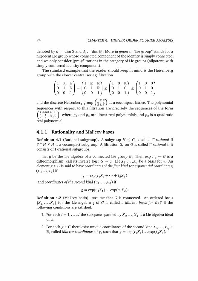
74 CHAPTER 4. HIGHER ORDER FOURIER ANALYSIS
denoted by d := dim G and di := dim Gi . More in general, “Lie group” stands for anilpotent Lie group whose connected component of the identity is simply connected,and we only consider (pre-)filtrations in the category of Lie groups (nilpotent, withsimply connected identity component).
The standard example that the reader should keep in mind is the Heisenberggroup with the (lower central series) filtration
1 R R0 1 R0 0 1
=
1 R R0 1 R0 0 1
≥
1 0 R0 1 00 0 1
≥
1 0 00 1 00 0 1
and the discrete Heisenberg group
1 Z Z0 1 Z0 0 1
as a cocompact lattice. The polynomialsequences with respect to this filtration are precisely the sequences of the form
1 p1(n) p2(n)0 1 p3(n)0 0 1
, where p1 and p3 are linear real polynomials and p2 is a quadratic
real polynomial.
4.1.1 Rationality and Mal’cev bases
Definition 4.1 (Rational subgroup). A subgroup H ≤ G is called Γ-rational ifΓ∩ H ≤ H is a cocompact subgroup. A filtration G• on G is called Γ-rational if itconsists of Γ-rational subgroups.
Let g be the Lie algebra of a connected Lie group G. Then exp : g → G is adiffeomorphism; call its inverse log : G → g. Let X1, . . . , Xd be a basis for g. Anelement g ∈ G is said to have coordinates of the first kind (or exponential coordinates)(t1, . . . , td) if
g = exp(t1X1 + · · ·+ td Xd)
and coordinates of the second kind (u1, . . . , ud) if
g = exp(u1X1) . . . exp(ud Xd).
Definition 4.2 (Mal’cev basis). Assume that G is connected. An ordered basisX1, . . . , Xd for the Lie algebra g of G is called a Mal’cev basis for G/Γ if thefollowing conditions are satisfied.
1. For each i = 1, . . . , d the subspace spanned by X i , . . . , Xd is a Lie algebra idealof g.
2. For each g ∈ G there exist unique coordinates of the second kind t1, . . . , td1∈
R, called Mal’cev coordinates of g, such that g = exp(t1X1) . . . exp(td Xd).
4.1. NILMANIFOLDS AND NILSEQUENCES 75
3. The lattice Γ consists precisely of the elements with integer Mal’cev coordi-nates.
Let G• be a filtration of length l on G that consists of connected, simply connectedLie groups. The Mal’cev basis X1, . . . , Xd is said to be adapted to G• if the followingadditional condition is satisfied.
4. For each i = 1, . . . , l the Lie algebra of Gi coincides with¬
Xd−di+1, . . . , Xd
¶
.
For not necessarily connected G and Gi a Mal’cev basis for G/Γ (adapted to G•) is aMal’cev basis for Go/Γo (adapted to Go
• ).
By a result of Mal’cev [Mal49] there always exists a Mal’cev basis adapted to thelower central series. Using this fact we can explain the name “rational subgroup” asfollows.
Lemma 4.3. Assume that G is connected and let H ≤ G be a connected Lie subgroupwith Lie algebra h. Then the following statements are equivalent.
1. The subgroup H is Γ-rational.
2. logΓ∩ h is a lattice in the Lie algebra h.
3. The Lie algebra h is spanned by rational combinations of vectors in a Mal’cevbasis for G/Γ.
Proof. Assume that (1) holds. Mal’cev’s result then implies existence of a Mal’cevbasis for H/(H ∩Γ), which in particular implies (2). It is clear that (2) implies (3).Finally, one may assume that the rational linear combintations in (3) are in factinteger linear combinations, and using properties of a Mal’cev basis this can be usedto find a relatively compact fundamental domain for exp |h mod Γ, proving (1).
4.1.2 Commensurable lattices
Lemma 4.4. Let G/Γ be a nilmanifold and Γ≤ G be a group that is commensurablewith Γ. Then the following assertions hold.
1. Γ is also a discrete cocompact subgroup.
2. Every Γ-rational subgroup G′ ≤ G is also Γ-rational.
76 CHAPTER 4. HIGHER ORDER FOURIER ANALYSIS
Proof. To see (1) note that if Γ≤ Γ, then the natural map G/Γ→ G/Γ is a coveringmap with finitely many sheets, and it follows that G/Γ is compact. If Γ ≤ Γ, thenG/Γ is a quotient space of G/Γ, so it is clearly compact. From this it follows that Γis cocompact in general. Also, it is clear that Γ is discrete if and only if Γ is discrete.
The assertion (2) follows since the groups Γ∩G′ and Γ∩G′ are commensurablewhenever Γ and Γ are commensurable.
An important class of examples of commensuarble lattices arises when one needsto replace a nilmanifold by a connected one.
Lemma 4.5. Let G/Γ be a nilmanifold and G• a Γ-rational filtration. Then thereexists a lattice Γ≤ Γ≤ G such that Γ has finite index in Γ and Gi/Γi is connected forevery i.
Proof. We use induction on the length of the filtration. If G• is trivial, then there isnothing to show, so suppose that the conclusion holds for filtrations of length d − 1and consider a Γ-rational filtration G• of length d.
By the rationality assumption we can write Gd = God ⊕ A in such a way that
Γ∩ A≤ A is a finite index subgroup. Since A is central in G, this implies that Γ hasfinite index in ΓA. Replacing Γ by ΓA if necessary, we may assume that ΓGd = ΓGo
d .By the inductive assumption ΓGd/Gd is a finite index subgroup of a lattice Γ/d
such that (Gi/Gd)/Γ/d is connected for every i. Let γ j ⊂ G/Gd be a finite setthat together with ΓGd/Gd generates Γ/d . We can write γ j = g jGd , and we haveg r
j ∈ ΓGd for some r and all j. Now recall that ΓGd = ΓGod and that in the connected
commutative Lie group God arbitrary roots exist. Hence, multiplying g j by an element
of God if necessary, we may assume that g r
j ∈ Γ.By Corollary 1.15 Γ has finite index in the group generated by Γ and the
elements g j . It remains to show that Gi/Γi is connected for every i. Recall that bythe inductive assumption the quotient Gi/ΓiGd = Gi/ΓiG
od is connected, hence path
connected. Since the quotient of Gi/Γi by continuous action of the path connectedgroup Go
d is path connected, Gi/Γi is connected.
SincepΓ≤ commG(Γ), Lemma 4.4 has the following consequence.
Corollary 4.6. Let G/Γ be a nilmanifold and G′ ≤ G a Γ-rational subgroup. Then forevery γ ∈
pΓ the subgroup γ−1G′γ is Γ-rational.
It is also useful to know what the conjugation map looks like in coordinates.
Lemma 4.7. Let G/Γ be a nilmanifold with a Mal’cev basis adapted to G• and γ ∈pΓ.
Then the conjugation map g 7→ γ−1 gγ is linear, unipotent, and upper triangular with
4.1. NILMANIFOLDS AND NILSEQUENCES 77
rational coefficients in coordinates of the first kind on Go, and it is polynomial withrational coefficients in coordiantes of the second kind.
If in addition Go is commutative and γ ∈ Γ, then the conjugation map is linear andunipotent with integer coefficients in coordinates of the first and the second kind.
Proof. We have γr ∈ Γ for some r ∈ N>0. The conjugation map is conjugated toAd(γ) by the exponential map, so it is linear in coordinates of the first kind. It isunipotent and upper triangular in coordinates of the first kind since G is nilpotent.
Suppose that Ad(γ) has an irrational coefficient in coordinates of the first kind.Then Ad(γ)r = Ad(γr) also has an irrational coefficient. In view of the uppertriangular form of the coordinate change maps between coordinates of the first andthe second kind [GT12, (A.2)], this implies that the r-th power of the conjugationmap, written in coordinates of the second kind, maps some point of Zdim G to apoint with an irrational coordinate. This is a contradiction, since conjugation by anelement of Γ preserves Γ.
By [GT12, Lemma A.2] this implies that the conjugation map is polynomial withrational coefficients in coordinates of the second kind.
If Go is commutative, then coordinates of the first and the second kind coincide,so in the case γ ∈ Γ the above argument shows that the conjugation map has integercoefficients in coordinates of both kinds.
For completeness we also specialize this result to nilmanifolds whose structuregroup’s connected component of the identity is commutative. This is most useful inconjunction with Corollary 4.34.
Lemma 4.8 ([FK05, Proposition 3.1]). Let X = G/Γ be a connected nilmanifold andsuppose that Go is commutative. Then there is a homomorphism X ∼= Td such that forevery a ∈ G the map x 7→ ax is conjugated to a unipotent affine transformation on Td ,that is, there exists a nilpotent integer matrix N and a constant b ∈ Td such that, withthe above identification, ax = x + N x + b.
Proof. Let d = dim G. Since Go is commutative, we have Go ∼= Rd , the Lie groupisomorphism being given by coordinates of the first or second kind (which coincide).With this identification we have (Γ∩ Go)∼= Zd .
Since X is connected, every element a ∈ G can be written as a = gγ with g ∈ Go,γ ∈ Γ. In particular, X ∼= Go/Γ. For every h ∈ Go we have
ahΓ = g(γhγ−1)Γ.
The conjugation map by γ is unipotent with integer coefficients in coordinates of thesecond kind by Lemma 4.7, and multiplication by g is a translation in coordinatesof the second kind.
78 CHAPTER 4. HIGHER ORDER FOURIER ANALYSIS
4.1.3 Cube construction
We outline a special case of the cube construction of Green, Tao, and Ziegler [GTZ12,Definition B.2] using notation of Green and Tao [GT12, Proposition 7.2]. We willonly have to perform it on filtrations, but even in this case the result is in generalonly a prefiltration.
Definition 4.9 (Cube filtration). Given a prefiltration G• we define the prefiltrationG• by
Gi := Gi ×Gi+1Gi =
D
G4i , Gi+1 × Gi+1
E
= (g0, g1) ∈ Gi × Gi : g−10 g1 ∈ Gi+1,
where G4 = (g0, g1) ∈ G2 : g0 = g1 is the diagonal group corresponding to G. Byan abuse of notation we refer to the filtration obtained from G• by replacing G0with G1 as the “filtration G• ”.
To see that this indeed defines a prefiltration let x ∈ Gi , y ∈ Gi+1, u ∈ G j ,v ∈ G j+1, so that (x , x y) ∈ Gi and (u, uv) ∈ Gj . Then [(x , x y), (u, uv)] =([x , u], [x y, uv]) ∈ Gi+ j by (1.4) (or see [GT12, Proposition 7.2]).
For induction purposes it is important to know that G• is rational provided thatG• is. This follows from the next lemma.
Lemma 4.10 (Rationality of the cube filtration). Let G• be a Γ-rational filtration.Then the filtration
G20 = G2
1 ≥ G1 ≥ G22 ≥ G2 ≥ · · · ≥ G2
l ≥ Gl ≥ G2l+1 = 1G×G.
is Γ2-rational. In particular, Γ = Γ2 ∩ G1 is a cocompact lattice in G1 and thefiltration G• is Γ-rational.
Proof. Observe first that (G• )o = (Go
• ), since both these prefiltrations consist of
closed connected subgroups of G2 whose Lie algebras coincide. The existence of therequired Mal’cev basis follows from a result of Green and Tao [GT12, Lemma 7.4].Clearly, Γ2
i is cocompact in G2i for every i = 1, . . . , l.
It remains to show that Γi = Γ2 ∩ Gi is cocompact in Gi for every i = 1, . . . , l.
The existence of an adapted Mal’cev basis implies that Γ2 ∩ (Gi )o is cocompact in
(Gi )o. Let Γ≥ Γ be the finite index surgroup provided by Lemma 4.5. Writing
Γi =¬
(Γi)4, (Γi+1)
2¶
4.1. NILMANIFOLDS AND NILSEQUENCES 79
we see that Γi is a finitely generated subgroup ofp
Γi , so it is a finite index surgroupof Γi by Corollary 1.15. On the other hand,
Gi =¬
(Goi Γi)
∆, (Goi+1Γi+1)
2¶
= (Gi )oΓi ,
so that Gi /Γi is connected. By the above it is compact, and in view of Lemma 4.4
this implies that Gi /Γ is compact.
Lemma 4.11. Let g ∈ P(Z, G•). Then for every k ∈ Z the map
gk (n) := (g(n+ k), g(n))
is G• -polynomial.
Proof. We use induction on the length l of the prefiltration G•. Indeed, for l =−∞there is nothing to show. If l ≥ 0, then gk takes values in G0 since g(n)−1 g(n+k) =Dk g(n) ∈ G1 by definition of a polynomial. Moreover Dk′(g
k ) = (Dk′ g)
k (n), so that
Dk′(gk ) is G•+1-polynomial by the induction hypothesis.
4.1.4 Vertical characters
Let G/Γ be a nilmanifold and G• a Γ-rational filtration of length l. Then G/Γ is asmooth principal bundle with the compact commutative Lie structure group Gl/Γl .The fibers of this bundle are called “vertical” tori (as opposed to the “horizontal”torus G/ΓG2) and everything related to Fourier analysis on them is called “vertical”.
Definition 4.12 (Vertical character). Let G/Γ be a nilmanifold and G• a Γ-rationalfiltration on G. A measurable function F on G/Γ is called a vertical character if thereexists a character χ ∈×Gl/Γl such that for every gl ∈ Gl and a.e. y ∈ G/Γ we haveF(gl y) = χ(glΓl)F(y).
Definition 4.13 (Vertical Fourier series). Let G/Γ be a nilmanifold and G• be aΓ-rational filtration on G. For every F ∈ L2(G/Γ) and χ ∈×Gl/Γl let
Fχ(y) :=
∫
Gl/Γl
F(gl y)χ(gl)dgl . (4.14)
With this definition Fχ is defined almost everywhere and is a vertical characteras witnessed by the character χ. The usual Fourier inversion formula implies thatF =
∑
χ∈×Gl/ΓlFχ in L2(G/Γ). We further need the following variant of Bessel’s
inequality.
80 CHAPTER 4. HIGHER ORDER FOURIER ANALYSIS
Lemma 4.15 (Bessel-type inequality for vertical Fourier series). Let p ∈ [2,∞) andF ∈ Lp(G/Γ). Then
∑
χ
‖Fχ‖pLp(G/Γ) ≤ ‖F‖
pLp(G/Γ).
Note that the analogue for p =∞ follows immediately from (4.14).
Proof. Since vertical characters have constant absolute value on Gl/Γl -fibers, wehave by (4.14) and the Cauchy-Schwarz inequality
‖Fχ‖pLp(G/Γ) =
∫
G/Γ
∫
Gl/Γl
|Fχ(hhl)|2dhl · |Fχ(h)|p−2 dh
≤∫
G/Γ
∫
Gl/Γl
|Fχ(hhl)|2dhl
∫
Gl/Γl
|F(hhl)|2dhl
p/2−1dh
for every χ. By the Plancherel identity and Hölder’s inequality this implies
∑
χ
‖Fχ‖pLp(G/Γ) ≤
∫
G/Γ
∫
Gl/Γl
|F(hhl)|2dhl
p/2dh
≤∫
G/Γ
∫
Gl/Γl
|F(hhl)|pdhldh= ‖F‖pLp(G/Γ),
finishing the proof.
The correct analog of the Plancherel identity for vertical Fourier series reads∑
χ
‖Fχ‖2l
U l (G/Γ) = ‖F‖2l
U l (G/Γ),
where U l stands for appropriate Gowers-Host-Kra seminorms, see Eisner and Tao[ET12, Lemma 10.2] for the case l = 3.
Definition 4.16 (Sobolev space). Let G/Γ be a nilmanifold with a Γ-rational filtra-tion, so in particular we have a Mal’cev basis X1, . . . , Xd for the Lie algebra of G.We identify the vectors X i with their extensions to right invariant vector fields onG/Γ. The Sobolev space W j,p(G/Γ), j ∈ N, 1≤ p <∞, is defined by the norm
‖F‖pW j,p(G/Γ)
=j∑
a=0
d∑
b1,...,ba=1
‖X b1. . . X ba
F‖pLp(G/Γ).
4.1. NILMANIFOLDS AND NILSEQUENCES 81
We will write A®D B if A and B satisfy the inequality A≤ CB with some constantC that depends on some auxiliary constant(s) D and some geometric data.
Lemma 4.17 (Control on Sobolev norms in a vertical Fourier series). Let j ∈ N andp ∈ [2,∞). For every smooth function F on G/Γ we have
∑
χ
‖Fχ‖W j,p(G/Γ) ® j,p ‖F‖W j+dl ,p(G/Γ).
Proof. The compact abelian Lie group Gl/Γl is isomorphic to a product of a torus anda finite group. In order to keep notation simple we will consider the case Gl/Γl
∼= Tdl ,the conclusion for disconnected Gl/Γl follows easily from the connected case. Werescale the last dl elements of the Mal’cev basis in such a way that they correspond tothe unit tangential vectors at the origin of the torus Tdl . The characters on Gl/Γl arethen given by χm(z1, . . . , zm) = zm1
1 · · · · · zmdldl
with m= (m1, . . . , mdl) ∈ Zdl . Observe
that by (4.14) and the commutativity of Gl we have (∂i F)m = ∂i(Fm) = mi Fm forevery i and m, where ∂i denotes the derivative along the i-th coordinate in Tdl .Therefore, by Hölder’s inequality and Lemma 4.15
∑
m1,...,mdl6=0
‖Fχm‖Lp
p=
∑
m1,...,mdl6=0
1
|m1 · · ·mdl|‖m1 · · ·mdl
Fχm‖Lp
p
≤
∑
m1,...,mdl6=0
1
m1 · · ·mdl
pp−1p−1∑
m
‖m1 · · ·mdlFχm‖p
Lp
®∑
m
‖∂1 . . .∂dlFχm‖p
Lp ≤ ‖∂1 . . .∂dlF‖p
Lp ≤ ‖F‖pW dl ,p .
By the centrality of Gl the operations of taking derivatives along elements of theMal’cev basis and taking the χ-th vertical character (4.14) commute, so we have
∑
m1,...,mdl6=0
‖Fχm‖W j,p ® ‖F‖W j+dl ,p
for every j ∈ N. The same argument works if some of the indices (m1, . . . , mdl)
vanish, in which case a smaller number of derivatives is added to j, and thusaltogether
∑
m
‖Fχm‖W j,p ® ‖F‖W j+dl ,p .
82 CHAPTER 4. HIGHER ORDER FOURIER ANALYSIS
We will need an estimate on the L∞ norm of a vertical character in terms ofa Sobolev norm with minimal smoothness requirements. To this end we wouldlike to use a Sobolev embedding theorem on G/ΓGl , since this manifold has lowerdimension than G/Γ. Morally, a vertical character is a function on the base spaceG/ΓGl that is extended to the principal Gl/Γl -bundle G/Γ in a multiplicative fashion.However, in general this bundle lacks a global cross-section, so we are forced towork locally.
Lemma 4.18 (Sobolev embedding). Let G/Γ be a nilmanifold and G• a Γ-rationalfiltration of length l on G. Then for every 1 ≤ p ≤ ∞ and every vertical characterF ∈W d−dl ,p(G/Γ) we have
‖F‖∞ ®p ‖F‖W d−dl ,p ,
where the implied constant does not depend on F.
Proof. The case p =∞ is clear, so we may assume p <∞.Since Γ is discrete there exists a neighborhood U ⊂ G of the identity such that
the quotient map U → G/Γ is a diffeomorphism onto its image. Let M ⊂ G bea (d − dl)-dimensional submanifold that intersects Gl in eG transversely. By jointcontinuity of multiplication in G we may find neighborhoods of identity V ⊂ Gland W ⊂ M such that VW ⊂ U . By transversality the differential of the mapψ : V ×W → G, (v, w) 7→ vw is invertible at (eG , eG), so by the inverse functiontheorem and shrinking V, W if necessary we may assume that ψ is a diffeomorphismonto its image. We may also assume that V, W are connected, simply connectedand have smooth boundaries. Recalling that the quotient map U → G/Γ is adiffeomorphism, we obtain a chart Ψ : V ×W → G/Γ for a neighborhood of eGΓthat has the additional property that Ψ(gl v, w) = glΨ(v, w) whenever v, gl v ∈ V .Shrinking V and W further if necessary we may assume that the differential of Ψ andits inverse are uniformly bounded. By homogeneity we obtain similar charts for someneighborhoods of all points of G/Γ. By compactness G/Γ can be covered by finitelymany such charts, so it suffices to estimate ‖F‖L∞(imΨ) in terms of ‖F‖W d−dl ,p(imΨ).
By definition of Sobolev norms we have∫
v∈V
‖F Ψ‖pW d−dl ,p(v×W )
dv ® ‖F Ψ‖pW d−dl ,p(V×W )
® ‖F‖pW d−dl ,p(imΨ)
.
Since F is a vertical character and by multiplicativity of Ψ in the first argument, theintegrand on the left-hand side is constant, so that
‖F Ψ‖W d−dl ,p(v×W ) ® ‖F‖W d−dl ,p(imΨ) for all v ∈ V,
4.2. LEIBMAN’S ORBIT CLOSURE THEOREM 83
the bound being independent of v. Now, W is a d − dl dimensional manifold, so theusual Sobolev embedding theorem [AF03, Theorem 4.12 Part I Case A] applies andwe obtain
‖F Ψ‖L∞(v×W ) ® ‖F Ψ‖W d−dl ,p(v×W ) ® ‖F‖pW d−dl ,p(imΨ)
.
By the above discussion this implies the desired estimate.
4.2 Leibman’s orbit closure theorem
4.2.1 Nilsequences
With the advent of Host-Kra-Ziegler structure theory, nilsequences came to be seenas the basic structure block of measure-preserving dynamical systems.
Definition 4.19. Let G/Γ be a nilmanifold. Let further G• be a Γ-rational filtrationof length l on G. Then for every polynomial g ∈ P(Z, G•) and F ∈ C(G/Γ) wecall the sequence (F(g(n)Γ))n a basic l-step nilsequence. An l-step nilsequence is auniform limit of basic l-step nilsequences (which are allowed to come from differentnilmanifolds and filtrations).
Note that the groups in the filtration G• are not assumed to be connected. Infact, by the remark following [HK08, Theorem 3], not every nilsequence arises fromnilmanifolds associated to connected Lie groups. Nilsequences appear naturallyin connection with norm convergence of multiple ergodic averages [HK05]. The1-step nilsequences are exactly the almost periodic sequences. For examples anda complete description of 2-step nilsequences see Host and Kra [HK08]. For acharacterization of nilsequences of arbitrary step in terms of their local propertiessee [HKM10, Theorem 1.1].
Although it is possible to express basic nilsequences as basic nilsequences of thesame step associated to “linear” sequences of the form (gn)n (this is essentially due toLeibman [Lei05c], see e.g. Chu [Chu09, Proposition 2.1] or Green, Tao, and Ziegler[GTZ12, Proposition C.2] in the setting of connected Lie groups), “polynomial”nilsequences, in addition to being formally more general, seem to be better suitedfor inductive purposes. This has been observed recently and utilized in connectionwith additive number theory, see e.g. Green, Tao, and Ziegler [GTZ12] and Greenand Tao [GT10].
Clearly, one can replace P(Z, G•) by P0(Z, G•) in Definition 4.19. Indeed, ifg ∈ P(Z, G•) and F ∈ C(G/Γ), then
F(g(n)) = Fg(0)(g(0)−1 g(n)),
84 CHAPTER 4. HIGHER ORDER FOURIER ANALYSIS
where Fa(x) := F(ax) is another continuous function on G/Γ. Now the argument isa polynomial sequence that vanishes at zero.
In this construction we have ‖Fa‖∞ ≤ ‖Fa‖∞. Unfortunately, one cannot ingeneral estimate the norm of Fa in a function space (such as Sobolev space or thespace of Lipschitz functions) by the norm of F in the same space. A remedy consistsin restricting a to a relatively compact subset of G.
Lemma 4.20 (Fundamental domain). Let Γ≤ G be a cocompact lattice. Then thereexists a relatively compact set K ⊂ G and a map G→ K, g 7→ g such that gΓ = gΓand g= g for each g ∈ G.
This follows readily from local homeomorphy of G and G/Γ, from local com-pactness of G and from compactness of G/Γ. For example, for G = R and Γ = Zthe fundamental domain K can be taken to be the interval [0,1) with the usualfractional part map ·. In case of a general connected Lie group the fundamentaldomain can be taken to be [0, 1)d in Mal’cev coordinates [GT12, Lemma A.14], butwe do not need this information. For each nilmanifold that we consider we fix somemap · as above.
Using the fractional part map we can rewrite a nilsequence associated to g ∈P(Z, G•) and F ∈ C(G/Γ) as
F(g(n)) = Fg(0)(g(0)−1 g(n)g(0)−1g(0)).
This is made possible by the fact that g(0)−1g(0) ∈ Γ. Note that Fg(0) belongs toa compact subset of C(G/Γ) that does not depend on g.
Henceforth we will mostly consider nilsequences associated to polynomial se-quences that vanish at zero, keeping at mind that the general case can be treated bythe above trick.
A key tool for many inductive proofs is the following modification of a construc-tion due to Green and Tao, see e.g. [Tao12, Lemma 1.6.13] and [GT12, §7], whichshows that discrete derivatives of nilsequences associated to vertical characters arenilsequences of lower step. Let G• be a filtration of length l, g ∈ P0(Z, G•), andF ∈ C(G/Γ) be a vertical character. Then
F(g(n+ k))F(g(n)) = Fg(k)(gk (0)
−1 gk ),
where Fa (x , y) := F(ax)F(y). To see that this is a nilsequence of step l − 1, notethat the sequence gk is G• -polynomial by Lemma 4.11. Moreover, the functionFa is Gl -invariant since F is a vertical character, so we may factor by Gl , therebyreducing the length of the filtration.
4.2. LEIBMAN’S ORBIT CLOSURE THEOREM 85
This construction suffers from the deficiency outlined above, namely that thereis in general no control on Fa in terms of F . This can be resolved in the same wayas before, considering the G1 -valued G• -polynomial sequence
gk := (g(k)−1 g(n+ k)g(k)−1g(k), g(n)). (4.21)
Then we obtainF(g(n+ k))F(g(n)) = Fg(k)(g
k (n)).
We will sometimes abuse the notation and write Fk instead of Fg(k).
Lemma 4.22 (Control on Sobolev norms in the cube construction). With the abovenotation we have
‖Fk ‖W j,p(G/Γ) ® j,p ‖F‖2W j,2p(G/Γ) for any j ∈ N, p ∈ [1,∞), (4.23)
where the implied constant does not depend on k and F.
Proof. For the Mal’cev basis on G/Γ that is induced by the Mal’cev basis on G1 /Γ
we have‖Fk ‖W j,p(G/Γ) = ‖Fg(k) ⊗ F‖W j,p(G1 /Γ
),
so it suffices to estimate the latter quantity.To this end observe that the Haar measure on G1 /Γ
is a self-joining of the Haarmeasure on G/Γ under the canonical projections to the coordinates. Therefore andby the Cauchy-Schwarz inequality we have
‖F0 ⊗ F1‖2pLp(G1 /Γ
)=
∫
G1 /Γ
|F0(y0)F1(y1)|pdµG1 /Γ(y0, y1)
2
≤∫
G1 /Γ
|F0(y0)|2pdµG1 /Γ(y0, y1)
·∫
G1 /Γ
|F1(y1)|2pdµG1 /Γ(y0, y1)
=
∫
G/Γ
|F0|2pdµG/Γ
∫
G/Γ
|F1|2pdµG/Γ
= ‖F0‖2pL2p(G/Γ)‖F1‖
2pL2p(G/Γ)
86 CHAPTER 4. HIGHER ORDER FOURIER ANALYSIS
for any smooth functions F0, F1 on G/Γ. Now recall that g(k) ∈ K for some fixedcompact set K ⊂ G1, so that by smoothness of the group operation ‖Fg(k)‖L2p(G/Γ) ®‖F‖L2p(G/Γ). Similar calculations for the derivatives lead to the bound
‖Fg(k) ⊗ F‖W j,p(G1 /Γ) ® j,p ‖F‖2
W j,2p(G/Γ).
4.2.2 Reduction of polynomials to connected Lie groups
In the context of nilsequences it will sometimes be useful to replace G•-polynomialsequences by Go
• -polynomial sequences. As remarked earlier, this is not possible ingeneral. Here we show that this becomes possible upon passing to an appropriatesubsequence.
Given a prefiltration G• we define a prefiltration Go• by Go
i = Goi .
Lemma 4.24. Let X = G/Γ be a nilmanifold and G• a Γ-rational filtration. Assumethat Gi/Γi is connected for each i. Then every G•-polynomial sequence g(n) can bewritten in the form
g(n) = go(n)γ(n),
where go is a Go• -polynomial sequence, and γ is a Γ•-polynomial sequence.
Proof. We use induction on the length of the filtration G•. If G• has length 0, theng ≡ id, so we can take go = γ≡ id. Suppose therefore that the conclusion is knownfor filtrations of length d − 1 and consider a filtration G• of length d.
By the induction hypothesis applied to the filtration G•/d we can write
g(n)Gd = go/d(n)γ/d(n),
where go/d is a (G•/d)o-polynomial sequence and γ/d is a Γ•/Gd -polynomial sequence.
Since (Gi/Gd)o is covered by Goi for every i, we can lift go
/d to a Go• -polynomial
sequence go (here “lift” means that go/d = goGd). Also, we can clearly lift γ/d to a
Γ•-polynomial sequence γ.It follows that h= g(goγ)−1 is a G•-polynomial sequence with values in Gd . By
the rationality and connectedness assumption we can write Gd = God ⊕ A with A≤ Γ.
Splitting h= hohΓ accordingly and replacing go and γ by goho and γhΓ, respectively,we obtain the claim.
Lemma 4.25. Let G be a nilpotent group with a filtration G• and let Γ≤ G be a finiteindex subgroup. Then for every G•-polynomial sequence g(n) the sequence g(n)Γ isperiodic.
4.2. LEIBMAN’S ORBIT CLOSURE THEOREM 87
Proof. Replacing Γ by a finite index subgroup that is normal in G and workingmodulo Γ, we may assume that G is finite and Γ is trivial.
We use induction on length d of G•. If d = 0, then the conclusion holds trivially.If d > 0, then by the induction hypotesis the discrete derivative D1 g is periodic, andthe conclusion follows.
Corollary 4.26. Let G/Γ be a nilmanifold with a Γ-rational filtration G•. Then thereexists a lattice Γ such that Γ is a finite index subgroup of Γ and every G•-polynomialsequence g can be written in the form g = goγ, where go is Go
• -polynomial and γ isΓ•-polynomial. In particular, γΓ is periodic.
Proof. Consider Γ given by Lemma 4.5. The required splitting is provided byLemma 4.24. The claimed periodicity follows from Lemma 4.25.
4.2.3 Equidistribution criterion
Recall that a sequence (xn) in a regular measure space (X ,µ) is called
1. equidistributed on X if for every f ∈ C(X ) we have
limN→∞
1
N
N∑
n=1
f (xn) =
∫
f dµ,
2. well-distributed on X if for every Følner sequence (ΦN ) in Z and every f ∈ C(X )we have
limN→∞En∈ΦN
f (xn) =
∫
f dµ,
3. totally equidistributed on X if its restriction to every arithmetic progressionaZ+ b, 0≤ b < a, in Z is equidistributed on X , and
4. totally well-distributed on X if its restriction to every arithmetic progression inZ is well-distributed on X .
Leibman’s equidistribution criterion tells that the only obstruction to total well-distribution of G•-polynomial sequences on a connected nilmanifold G/Γ are hori-zontal characters, that is, continuous homomorphisms η : G→ R such that η(Γ)⊂ Z(see Theorem 4.30 for the precise formulation). We will give a qualitative version ofthe proof that is due to Green and Tao [GT12]. For reader’s convenience we willkeep the notation as close to [GT12] as possible.
88 CHAPTER 4. HIGHER ORDER FOURIER ANALYSIS
The proof proceeds by induction on the length of the filtration. In each stepone performs the cube construction and factors out the diagonal central subgroup.The induction hypothesis gives some information about horizontal characters onG. The next lemma describes how such horizontal characters induce horizontalcharacters on G.
Lemma 4.27. Let G/Γ be a nilmanifold with a Γ-rational filtration G•. Let η : G→R be a horizontal character. Then the map
η1 : G→ R, g 7→ η(g, g)
is a horizontal character on G/Γ, the map
η2 : G2→ R, g 7→ η(g, id)
is a horizontal character on G2/Γ2 such that η2([G, G2]) = 0 and the map (x , y) 7→η2([x , y]) is a bihomomorphism (that is, a group homomorphism in each variablewhen the other variable is fixed).
In particular, the map g 7→ η2([g,γ]) is a horizontal character on G/Γ for everyγ ∈ Γ.
Proof. It is clear that η1 and η2 are horizontal characters. For any g ∈ G, h ∈ G2 wehave
η2([g, h]) = η((g−1h−1 gh, id)) = η((g, g)−1(h, id)−1(g, g)(h, id))=−η(g, g)−η(h, id) +η(g, g) +η(h, id) = 0,
hence η2([G, G2]) = 0 (note that the restriction h ∈ G2 in the above calculationis necessary because otherwise (h, id) 6∈ G). This, together with the commutatoridentity (1.4), also shows that the map (x , y) 7→ η2([x , y]) is a bihomomorphism.
The main step in the proof of the equidistribution criterion is the followingtrichotomy that allows one to transfer information from the cube spaces to theoriginal nilmanifold. We have nothing to add to the proof in [GT12, §7].
Proposition 4.28. Let G/Γ be a nilmanifold and G• a Γ-rational filtration on Gconsisting of connected groups. Let g ∈ P0(Z, G•) be such that g(1) = g(1) andsuppose that there is a set of h of upper Banach density at least δ and a non-trivialhorizontal character η : G → R such that η(gh (Z)) ⊂ Z. Then at least one of thefollowing statements holds.
4.2. LEIBMAN’S ORBIT CLOSURE THEOREM 89
1. The map η1 is a non-trivial horizontal character and η1(g(Z))⊂ Z.
2. There exists i = 1, . . . , d such that the map ηi : G→ R, g 7→ η2([g, exp X i]), isa non-trivial horizontal character and qηi(g(Z))⊂ Z for some natural numberq that is bounded in terms of δ.
3. The map η2 : G2→ R is a non-trivial horizontal character and qη2(g2(Z))⊂ Zfor some natural number q that is bounded in terms of δ, where g2 is defined byg(n) = g(1)n g2(n).
The next result shows what happens if a polynomial sequence fails to be well-distributed. This is a qualitative version of the main result from [GT12], but wenote that not all quantitativity has been removed. In fact, it is essential for inductivepurposes to have some uniformity over all polynomials.
Theorem 4.29. Let G/Γ be a nilmanifold associated to a connected group G andG• a Γ-rational filtration on G. Let a Følner sequence (ΦN ) in Z, a function F ∈C(G/Γ) with
∫
F = 0, δ > 0, s ∈ N, and 0 ≤ r < s be given. Then there exists afinite set of non-trivial horizontal characters such that for every g ∈ P0(Z, G•) withlimsupN |En∈ΦN
F(g(sn+ r)Γ)| > δ there exists a horizontal character η on this listsuch that η(g(Z))⊂ Z.
Proof. We use induction on the length l of the filtration and the dimension d2 of thegroup G2.
First we reduce to the case that G• consists of connected groups. To this end wesplit g = goγ as in Corollary 4.26, where go is Go
• -polynomial and γ is Γ•-polynomialfor some finite index surgroup Γ≥ Γ that does not depend on g. In particular, γΓ isperiodic, and the period s′ does not depend on g. By the pigeonhole principle thereexists 0≤ r ′ < s′ such that
lim supN|En∈(ΦN−r ′)/s′ F(g(s(s
′n+ r ′) + r))|> δ,
and we can apply the connected case of the theorem. Thus we may assume that thefiltration G• consists of connected groups.
Next we show that we may assume s = 1, r = 0. In general our assumption canbe rewritten as
lim supN|En∈ΦN
Fg(r)(g(r)−1 g(sn+ r)g(r)−1g(r))|> δ.
Since g(r) lies in a fixed compact set, the set of functions Fg(r) that may appearabove is compact, so it can be covered by finitely many balls of radius δ/2, the
90 CHAPTER 4. HIGHER ORDER FOURIER ANALYSIS
covering being independent of g. Hence there is a finite set of continuous functionson G/Γ such that we have
limsupN|En∈ΦN
F(g(r)−1 g(sn+ r)g(r)−1g(r))|> δ/2
for one of the functions F in this set. We can now apply the s = 1, r = 0 case ofthe theorem to the polynomial sequence (g(r)−1 g(sn+ r)g(r)−1g(r))n and thefunction F . This provides us with a finite set of horizontal characters, for one ofwhich we have
η(g(r)−1 g(sZ+ r)g(r)−1g(r))⊂ Z.
This immediately implies η(g(sZ+r)g(r)−1)⊂ Z. Now the sequence (η(g(n)g(r)−1))nis a polynomial of degree at most l that takes integer values on the arithmetic pro-gression sZ+ r. Hence, multiplying η by a natural number that does not depend ong if necessary, we may assume η(g(Z)g(r)−1)⊂ Z. In view of g(0) = id this impliesη(g(Z))⊂ Z as required. Hence we may assume that s = 1, r = 0.
It remains to prove the conclusion under the additional assumptions that G•consists of connected groups, s = 1, and r = 0. Replacing g by the sequence
g(n)(g(1)−1 g(1))−n
we may also assume that g(1) = g(1). By uniform approximation we may assumethat F is smooth (this can be achieved for example using a smooth partition ofidentity and working locally).
If l = 1, then G/Γ is a torus. Smoothness implies that the Fourier seriesF =
∑
χ Fχ converges absolutely, so we may truncate it to a finite number ofsummands. Given a polynomial g as in the hypothesis, by the pigeonhole principlewe see that
lim supN|En∈ΦN
Fχ(g(n)Γ)|> 0
for one of the (finitely many) Fourier components Fχ . We may assume |Fχ | ≡ 1.Then we have Fχ(g(n)Γ) = Fχ(g(1)Γ)n, and the Kronecker equidistribution criterionimplies that (Fχ gΓ) ≡ 1. The character Fχ lifts to a horizontal character on G,and we obtain the claim.
Suppose now that l ≥ 2. Analogously to the commutative case, smoothnessimplies that the vertical Fourier series F =
∑
χ Fχ (Definition 4.13) convergesabsolutely, so, decreasing δ if necessary, we can assume that F has a verticalfrequency χ. If this frequency vanishes, then we can factor out Gl and use inductionon the length of filtration.
4.2. LEIBMAN’S ORBIT CLOSURE THEOREM 91
Assume now that the vertical frequency χ is non-trivial. By the van der Corputlemma (Lemma 4.52) the set of h such that
limsupN|En∈ΦN
F(g(h+ n))F(g(n))|> δ
has positive upper Banach density. Recall that the above can be written as
limsupN|En∈ΦN
Fh (gh (n))|> δ.
Since the fractional part function · has relatively compact range, the set of func-tions Fh is relatively compact. Choosing a sufficienttly fine finite covering of thisset, pigeonholing and decreasing δ if necessary we obtain one function Fa such that
lim supN|En∈ΦN
Fa (gh (n))|> δ
for a set of h of positive upper Banach density. Note that Fa has a non-trivial verticalfrequency with respect to G2
l and is G∆l -invariant. Hence, factoring out G∆l , we seethat gh is polynomial with respect to the filtration G• /G
∆l that has length l − 1 and
Fa has zero integral.By the induction hypothesis we obtain a finite list of horizontal characters
η : G/G∆l → R such that for each h in out positive upper Banach density set thereexists a character on this list with η(gh (Z)) ⊂ Z. By the pigeonhole principle wemay assume that the character η does not depend on h.
We are now in position to apply Proposition 4.28. If the first or the secondalternative from that proposition holds, then we are done, since the horizontalcharacters provided by that alternatives only depend on η. It remains to considerthe case that the last alternative from that proposition holds. In this case g isG′•-polynomial, where the filtration G′• is defined by G′1 = G1, G′i = Gi ∩ η−1
2 (1qZ)
for i ≥ 2 (the fact that this is a filtration follows from Lemma 4.27). Note thatdim G′2 < dim G2 since η2 is a non-trivial horizontal character on G2.
Now we bootstrap the last result to total well-distribution.
Theorem 4.30 (Leibman’s equidistribution criterion, connected case). Let G/Γ bea nilmanifold associated to a connected group G and G• a Γ-rational filtration on G.Then for every g ∈ P0(Z, G•) exactly one of the following alternatives holds.
1. For every subgroup Γ≤ G that is commensurable with Γ the sequence g(n)Γ istotally well-distributed on G/Γ or
92 CHAPTER 4. HIGHER ORDER FOURIER ANALYSIS
2. there exists a non-trivial horizontal character η : G→ R such that η(g(Z))⊂ Z.
Proof. It is clear that the two statements are mutually exclusive, so it suffices toshow that at least one of them holds. Suppose that the first statement fails, thatis, there exists a subgroup Γ ≤ G that is commensurable with G, an arithmeticprogression sZ+ r, a Følner sequence (ΦN ), and a function F ∈ C(G/Γ) such that
En∈ΦNF(g(sn+ r)Γ) 6→
∫
G/Γ
F as N →∞.
Without loss of generality we may assume∫
F = 0. By Theorem 4.29 we obtain anon-trivial horizontal character η on G/Γ such that η(g(Z))⊂ Z. Note that η takesinteger values on the finite index subgroup Γ∩ Γ ≤ Γ, from which it follows thatη(Γ)⊂ 1
RZ for some R. Hence η= Rη is a non-trivial horizontal character on G/Γ
such that η(g(Z))⊂ Z.
4.2.4 Leibman’s orbit closure theorem
In order to describe the orbit closure of a polynomial in a nilmanifold we need onemore decomposition result for polynomials.
Lemma 4.31. Let G/Γ be a nilmanifold with a Γ-rational filtration G• and H ≤ G arational subgroup. Then for every h ∈ P0(Z, H•) there exists a closed connected rationalsubgroup H ≤ H such that h can be written in the form h= hoγ, where γ ∈ P0(Z,
pΓ•),
ho ∈ P0(Z, Ho• ), and for every subgroup Γ ≤ G that is commensurable with Γ the
sequence hoΓ is totally well-distributed on H/Γ.
It clearly suffices to obtain the conclusion for H = G, the other cases are onlyneeded for the induction process.
Proof. We use induction on the dimension of H. If dim H = 0, then H ≤pΓ, and
we can set ho ≡ id, γ = h. Suppose now that the conclusion is known for rationalsubgroups of dimension < dim H.
Consider the splitting h = hoγ provided by Corollary 4.26 applied to the nil-manifold H/(H ∩ Γ). Replacing ho by hoho(0)−1 and γ by ho(0)γ we may assumeho(0) = γ(0) = id. Suppose that the conclusion of the lemma does not hold withH = Ho. Then Theorem 4.30 shows that ho takes values in a proper rationalsubgroup H ≤ Ho, namely the inverse image of Z under the horizontal characterfiguring in the second alternative in that theorem. In this case we can conclude bythe induction hypothesis.
4.2. LEIBMAN’S ORBIT CLOSURE THEOREM 93
Thus we have split an arbitrary polynomial into a “totally equidistributed” anda “rational” part. Further analysis of the rational part now yields Leibman’s orbitclosure theorem.
Theorem 4.32 (Leibman’s orbit closure theorem, cf. [Lei05c, Theorem B]). Let G/Γbe a nilmanifold with a Γ-rational filtration G•. Then for every G•-polynomial sequenceg there exists a closed connected Γ-rational subgroup H such that Z can be partitionedinto progressions on each of which g(n)Γ is totally well-distributed on g(0)Hc/Γ forsome c ∈
pΓ.
In order to obtain the precise statement of [Lei05c, Theorem B] one couldconsider g(0)H g(0)−1 instead of H. Note that this subgroup is in general notΓ-rational.
Proof. We may assume g(0) = id. Consider the group H and the splitting g = hoγprovided by Lemma 4.31. Since γ takes values in a finitely generated subgroup ofpΓ and by Lemma 4.25, we can split Z into arithmetic progressions Zi such thatγ(n)Γ = ciΓ for some ci ∈
pΓ and all n ∈ Zi .
By Lemma 4.31 the sequence hociΓc−1i |Zi
is totally well-distributed on H/(ciΓc−1i ).
By conjugation and translation invariance this implies that the sequence
gΓ|Zi= hociΓ|Zi
= cic−1i (h
ociΓc−1i )ci |Zi
is totally well-distributed on Hci/Γ⊂ G/Γ.
One immediate consequence is the pointwise ergodic theorem for polynomialsin nilmanifolds.
Corollary 4.33 ([Lei05c, Theorem A]). Let G/Γ be a nilmanifold, g a polynomialsequence, and f ∈ C(G/Γ). Then the limit UC-limn f (g(n)Γ) exists.
The other consequence is a well-distribution criterion. It shows that for manypurposes it suffices to consider nilmanifolds whose structure groups’ connectedcomponents of identity are commutative.
Corollary 4.34 ([Lei05c, Theorem C]). Let G/Γ be a connected nilmanifold witha Γ-rational filtration G•. Then for a G•-polynomial sequence g(n) the followingstatements are equivalent.
1. g(n)Γ is totally well-distributed on G/Γ,
2. g(n)Γ[Go, Go] is dense in G/Γ[Go, Go].
94 CHAPTER 4. HIGHER ORDER FOURIER ANALYSIS
The connectedness requirement cannot be removed as the example G = Z/2Z,g = (. . . , 1, 0, 0,0,1,0,0,0,1, . . . ), shows. This sequence is polynomial of degree 3and its image is all of G, but it is not equidistributed.
Proof. Both statements are invariant under multiplication by constants on the left,so we may assume g(0) = id.
(1) clearly implies (2). For the converse consider the subgroup H ≤ G providedby Theorem 4.32. If H ≤ Go is a proper subgroup, then it has lower dimension thanGo, so that g(n)Γ takes values in a finite union of submanifolds of G/Γ of strictlylower dimension, contradicting density. Hence Z splits into finitely many arithmeticprogressions, and the restriction of g(n)Γ to each of these progressions is totallywell-distributed on G/Γ. This implies the claim.
4.2.5 Nilsystems
A (k-step) nilsystem is a measure-preserving system of the form (X , T), whereX = G/Γ is a (k-step) nilmanifold and T gΓ = agΓ for some a ∈ G and all gΓ ∈ G/Γ.A k-step pro-nilsystem is an inverse limit of k-step nilsystems in the category ofmeasure-preserving systems (equivalently, in the category of topological dynamicalsystems with an invariant Borel probability measure [HKM10, Theorem A.1]). A(pro-)nilfactor of a measure-preserving dynamical system is a factor that is also a(pro-)nilsystem.
We will now state and prove an important characterization of ergodic nilsystems.For other proofs see [AGH63], [Par70], or [Lei05c, §2.17–2.20].
Lemma 4.35. Let X = (G/Γ, a) be a nilsystem. Then the following statements areequivalent.
1. X is topologically transitive as a topological dynamical system.
2. X is ergodic with respect to the Haar measure.
3. X is uniquely ergodic.
Proof. (3) clearly implies (2) since the Haar measure is invariant. (2) implies (1)since the Haar measure has full support.
Suppose now that (1) holds. It is easy to see that X is distal, cf. [Lei05c,Theorem 2.14]. Hence any two orbit closures in X either coincide or are disjoint. Bytopological transitivity at least one orbit is dense in X , so that every orbit is densein X . Fix an orbit (an x). It follows from Theorem 4.32 that Z splits into a finiteunion of arithmetic progressions in such a way that the restriction of the orbit to
4.3. BACKGROUND FROM ERGODIC THEORY 95
each of these progressions is totally well-distributed on a connected component ofX . By topological transitivity we know that a permutes the connected componentscyclically. It follows that (an x) is well-distributed with respect to the Haar measureon G/Γ.
It is a classical fact that the Kronecker factor of an ergodic nilsystem (G/Γ, T ) isthe canonical map G/Γ→ G/ΓG2, where G2 = [G, G]. The nilmanifold G/ΓG2 is acompact homogeneous space of the abelian Lie group G/G2, hence a disjoint unionof finitely many tori. The fibers of the projection G/Γ→ G/ΓG2 are isomorphic tothe homogeneous space G2/Γ2, where Γ2 = Γ∩ G2. By a result of Mal’cev Γ2 is acocompact subgroup of G2 [Mal49], so each such fiber is also a nilmanifold.
4.3 Background from ergodic theory
In this section we will state several results about the pointwise ergodic theorem,measure disintegration and Host-Kra-Ziegler factors. Not all of them are needed inthe proof of our Wiener-Wintner theorem, but they will come in handy in the nextchapter when we will be dealing with the return times theorem.
4.3.1 Følner sequences
Definition 4.36. Let G be a locally compact second countable group with left Haarmeasure | · |. A sequence of sets Φn ⊂ G is called
1. a (weak) Følner sequence if for every compact set K ⊂ G one has
|Φn∆KΦn|/|Φn| → 0 as n→∞,
2. a strong Følner sequence if for every compact set K ⊂ G one has
|∂K(Φn)|/|Φn| → 0 as n→∞,
where ∂K(Φ) = K−1Φ∩ K−1Φû is the K-boundary of Φ, and
3. (C-)tempered if there exists a constant C such that
| ∪i< j Φ−1i Φ j |< C |Φ j | for every j.
96 CHAPTER 4. HIGHER ORDER FOURIER ANALYSIS
Note that any of the above conditions implies that (Φn) is a Følner net in thesense of Definition 2.1.
Every strong Følner sequence is also a weak Følner sequence. In countablegroups the converse is also true, but already in R this is no longer the case: let forexample (Φn) be a sequence of nowhere dense sets Φn ⊂ [0, n] of Lebesgue measuren− 1/n, say. This is a weak but not a strong Følner sequence (in fact, ∂[−1,0]Φn isbasically [0, n+ 1]). However, a weak Følner sequence can be used to construct astrong Følner sequence.
Lemma 4.37. Assume that a locally compact second countable group G admits a weakFølner sequence. Then G also admits a strong Følner sequence.
Proof. We follow the argument in [PS12, Lemma 2.6]. Let (Vj) be a countablebasis for the topology of G that consists of relatively compact sets. Let K ⊂ G be acompact set, then it is covered by a finite union of Vj ’s. Hence we obtain a countableascending chain of compact subsets of G such that every compact subset is containedin one of the sets in this collection, namely the collection of KN := ∪N
j=1Vj .
Let N be arbitrary and set K := KN , ε := 1N
. It suffices to find a compact set Φwith |∂K(Φ)|/|Φ|< ε. Let (Φn) be a weak Følner sequence, then there exists n suchthat |K−1KΦn∆Φn|< ε|Φn|. Set Φ = KΦn, then
∂KΦ = K−1KΦn ∩ K−1(KΦn)û ⊂ K−1KΦn ∩Φûn,
and this has measure less than ε|Φn| ≤ ε|Φ|.
Since every weak (hence also every strong) Følner sequence has a temperedsubsequence [Lin01, Proposition 1.4], this implies that every lcsc amenable groupadmits a tempered strong Følner sequence.
4.3.2 Lindenstrauss covering lemma
Given a collection of intervals, the classical Vitali covering lemma allows one toselect a disjoint subcollection that covers a fixed fraction of the union of the fullcollection. The appropriate substitute in the setting of tempered Følner sequencesis the Lindenstrauss random covering lemma. It allows one to select a randomsubcollection that is expected to cover a fixed fraction of the union and to be almostdisjoint. The almost disjointness means that the expectation of the counting functionof the subcollection is uniformly bounded by a constant. As such, the Vitali lemma isstronger whenever it applies, and the reader who is only interested in the standardFølner sequence in Z can skip this subsection.
4.3. BACKGROUND FROM ERGODIC THEORY 97
We use two features of Lindenstrauss’ proof of the random covering lemma thatwe emphasize in its formulation below. The first feature is that the second moment(and in fact all moments) of the counting function is also uniformly bounded(this follows from the bound for the moments of a Poisson distribution). Thesecond feature is that the random covering depends measurably on the data. Wechoose to include the explicit construction of the covering in the statement of thelemma instead of formalizing this measurability statement. To free up symbols forsubsequent use we replace the auxiliary parameter δ in Lindenstrauss’ statement ofthe lemma by C−1 and expand the definition of γ.
For completeness we recall that a Poisson point process with intensity α on ameasure space (X ,µ) is a counting (i.e. atomic, with at most countably many atomsand masses of atoms in N) measure-valued map Υ : Ω→ M(X ) such that for everyfinite measure set A⊂ X the random variable ω 7→Υ(ω)(A) is Poisson with meanαµ(A) and for any disjoint sets Ai the random variables ω 7→ Υ(ω)|Ai
are jointlyindependent (here and later Υ|A is the measure Υ|A(B) = Υ(A∩B)). It is well-knownthat on every σ-finite measure space there exists a Poisson process.
Lemma 4.38 ([Lin01, Lemma 2.1]). Let G be a lcsc group with left Haar measure| · |. Let (ΦN )RN=L be a C-tempered sequence. Let ΥN : ΩN → M(G ) be independentPoisson point processes with intensity αN = δ/|ΦN | w.r.t. the right Haar measure ρ onG and let Ω :=
∏
N ΩN .Let AN |R+1 ⊂ G , N = L, . . . , R, be sets of finite measure. Define (dependent!)
counting measure-valued random variables ΣN : Ω→ M(G ) in descending order forN = R, . . . , L by
1. ΣN :=ΥN |AN |N+1,
2. Ai|N := Ai|N+1 \Φ−1i ΦNΣN = a ∈ Ai|N+1 : Φia ∩ΦNΣN = ; for i < N.
Then for the counting function
Λ =∑
N
ΛN , ΛN (g)(ω) =∑
a∈ΣN (ω)
1ΦN a(g)
the following holds.
1. Λ is a measurable, a.s. finite function on Ω×G ,
2. E(Λ(g)|Λ(g)≥ 1)≤ 1+ C−1 for every g ∈ G ,
3. E(Λ2(g)|Λ(g)≥ 1)≤ (1+ C−1)2 for every g ∈ G ,
98 CHAPTER 4. HIGHER ORDER FOURIER ANALYSIS
4. E(∫
Λ)≥ (2C)−1| ∪RN=L AN |.
Recall that the maximal function is defined by
M f (x) := supN
En∈ΦNf (T n x)
for f ∈ L1(X ).
The Lindenstrauss maximal inequality [Lin01, Theorem 3.2] asserts that for everyf ∈ L1(X ) and every λ > 0 we have
µM f > λ® λ−1‖ f ‖1, (4.39)
where the implied constant depends only on the constant in the temperednesscondition. This implies the following pointwise ergodic theorem.
Theorem 4.40 ([Lin01, Theorem 1.2]). Let G be a locally compact second countableamenable group with a tempered Følner sequence (ΦN ). Suppose that G measurablyacts on a probability space (X ,µ) by measure-preserving transformations. Then forevery f ∈ L1(X ,µ) there exists a full measure subset X ′ ⊂ X such that for every x ∈ X ′
the limit
limN→∞
1
|ΦN |
∫
g∈ΦN
f (g x)
exists. If the action is ergodic, then the limit equals∫
Xf dµ a.e.
The temperedness assumption cannot be dropped even for sequences of intervalswith growing length in Z, see del Junco and Rosenblatt [dJR79] and Rosenblatt andWierdl [RW92].
4.3.3 Fully generic points
Let (X ,G ) be an ergodic measure-preserving system and f ∈ L1(X ). Recall that apoint x ∈ X is called generic for f if
limn→∞Eg∈Φn
f (g x) =
∫
X
f .
In the context of countable group actions fully generic points for f ∈ L∞(X ) areusually defined as points that are generic for every function in the closed G -invariantalgebra spanned by f . For uncountable groups this is not a good definition, since
4.3. BACKGROUND FROM ERGODIC THEORY 99
this algebra need not be separable. The natural substitute for shifts of a functionf ∈ L∞(X ) is provided by convolutions
c ∗ f (x) =
∫
Gc(g−1) f (g x)dg, c ∈ L1(G ).
Since L1(G ) is separable and convolution is continuous as an operator L1(G )×L∞(X )→ L∞(X ), the closed convolution-invariant algebra generated by f is separa-ble.
We call a point x ∈ X fully generic for f if it is generic for every function in thisalgebra. In view of the Lindenstrauss pointwise ergodic theorem (Theorem 4.40), if(Φn) is tempered, then for every f ∈ L1(X ) a.e. x ∈ X is generic. Consequently, forevery f ∈ L∞(X ) a.e. x ∈ X is fully generic.
4.3.4 Ergodic decomposition
A measure-preserving system (X ,µ, T ) is called regular if X is a compact metric space,µ is a Borel probability measure and T is continuous. Every measure-preservingsystem is measurably isomorphic to a regular measure-preserving system uponrestriction to a separable T -invariant sub-σ-algebra [Fur81, §5.2].
The ergodic decomposition of the measure on a regular measure-preservingsystem (X ,µ, T) is a measurable map x 7→ µx from X to the space of T -invariantergodic Borel probability measures on X , unique up to equality µ-a.e., such thatµ-a.e. x ∈ X is generic for every f ∈ C(X ) w.r.t. µx and µ =
∫
µxdµ(x) [Fur81,§5.4]. Moreover, for every f ∈ L1(µ), for µ-a.e. x ∈ X we have that f ∈ L1(µx) andx is generic for f w.r.t. µx .
In connection with the multiple term return times theorem we find it illuminatingto think of the ergodic decomposition in a particular way (that will be generalized in§5.2.2). Let (X ,µ, T ) be a regular measure-preserving system. By the Lindenstrausspointwise ergodic theorem (Theorem 4.40) a.e. x ∈ X is generic for some T -invariantBorel probability measure mx on X , i.e. En∈ΦN
f (T n x)→∫
f dmx for every f ∈ C(X ).It follows easily that the function x 7→mx is measurable and
µ=
∫
mxdµ(x) (4.41)
In particular, for µ-a.e. x the measure my is defined for mx -a.e. y . To see that mx isergodic for µ-a.e. x it suffices to verify that
∫ ∫
∫
f dmy −∫
f dmx
2dmx(y)dµ(x) = 0 for every f ∈ C(X ), (4.42)
100 CHAPTER 4. HIGHER ORDER FOURIER ANALYSIS
since this says precisely that the ergodic averages of f converge pointwise mx -a.e. toan mx -essentially constant function for µ-a.e. x , and the latter full measure set canbe chosen independently from f since C(X ) is separable. By definition of mx , my ,the dominated convergence theorem and (4.41) we can rewrite the integral in(4.42) as
2 limN
∫
(En∈ΦNT n f )2(x)dµ(x)
− 2 limN
∫
(En∈ΦNT n f )(x)
∫
(En∈ΦNT n f )(y)dmx(y)dµ(x)
= 2 limN
∫
(En∈ΦNT n f )2(x)dµ(x)
− 2 limN
limM
∫
(En∈ΦNT n f )(x)(En∈ΦM
T m f )(x)dµ(x),
and this vanishes by the Lindenstrauss pointwise ergodic theorem (Theorem 4.40)and the dominated convergence theorem.
4.3.5 Host-Kra cube spaces
We recall the basic definitions and main results surrounding the uniformity semi-norms. Let (X ,µ, T) be a regular, not necesserily ergodic, measure-preservingsystem. The cube measures µ[l] on X [l] := X 2l
are defined inductively starting withµ[0] := µ. In the inductive step, given µ[l], fix an ergodic decomposition
µ[l] =
∫
X [l]mxdµ[l](x)
as in (4.41). The space on which mx is defined can be inferred from the subscript x .Define
µ[l+1] :=
∫
X [l]δx ⊗mxdµ[l](x). (4.43)
Using (4.41) and (4.42), we can write the above integral as
µ[l+1] =
∫ ∫
δy ⊗mydmx(y)dµ[l](x)
=
∫ ∫
δy ⊗mxdmx(y)dµ[l](x) =
∫
mx ⊗mxdµ[l](x), (4.44)
4.3. BACKGROUND FROM ERGODIC THEORY 101
which is the usual definition of the cube measures.
Definition 4.45 (Gowers-Host-Kra seminorms [HK05, §3.5]). The Gowers-Host-Kraseminorms, or uniformity seminorms, are defined by
‖ f ‖2l+1
U l+1(X ,µ,T ) :=
∫
⊗ε∈0,1l+1 f dµ[l+1] =
∫
E
⊗ε∈0,1l f |I [l]2dµ[l], (4.46)
where I [l] is the T [l]-invariant sub-σ-algebra on X [l].
We will write U l or U l(X ) instead of U l(X ,µ, T ) if no confusion is possible. In aspecial case these seminorms have been introduced by Bergelson [Ber00].
If µ=∫
µxdµ(x) is the ergodic decomposition, then
‖ f ‖2l
U l (X ,µ) =
∫
‖ f ‖2l
U l (X ,µx )dµ(x) for all f ∈ L∞(µ).
It follows from the mean ergodic theorem that the uniformity seminorms can berecursively computed by the following folmulas.
‖ f ‖U0(X ,µ) =
∫
X
f dµ, ‖ f ‖2l+1
U l+1(X ,µ) = limN→∞
1
N
N∑
n=1
‖T n f f ‖2l
U l (X ,µ).
For fε ∈ L∞(X ), ε ∈ 0,1l , we will abbreviate f [l] := ⊗ε∈0,1l fε. It follows byinduction on l ∈ N that
‖ · ‖U l+1(X ) ≤ ‖ · ‖L2l (X ), (4.47)
see [ET12] for subtler analysis. The uniformity seminorms satisfy the Cauchy-Schwarz-Gowers inequality [HK05, Lemma 3.9.(1)]
∫
f [l]dµ[l]
≤∏
ε∈0,1l‖ fε‖U l . (4.48)
For every l the uniformity seminorm U l+1 determines a factor Zl(X ) of (X ,µ, T ),called the Host-Kra factor of order l, that is characterized by the relation
‖ f ‖U l+1(X ) = 0 ⇐⇒ E( f |Zl(X )) = 0
that holds for all f ∈ L∞(X ). The structure of the factors Zl is captured by thefollowing result of Host and Kra.
102 CHAPTER 4. HIGHER ORDER FOURIER ANALYSIS
Theorem 4.49 ([HK05]). Suppose that (X ,µ, T ) is ergodic. ThenZl(X ) is measurablyisomorphic to a pro-nilsystem of step l.
We should like to mention that these factors have been also independentlyconstructed by Ziegler [Zie07].
In the non-ergodic case one could use this result on every ergodic component,but it is not clear in which sense the resulting pro-nilsystems vary measurablywith the ergodic component (some work on this problem has been done by Austin[Aus10]). At any rate, the following decomposition result of Chu, Frantzikinakis,and Host suffices for our purposes.
Theorem 4.50 ([CFH11, Proposition 3.1]). Suppose that f ∈ L∞(Zl) for some l.Then for every ε > 0 there exists a function fs ∈ L∞(Zl(X ),µ) such that ‖ fs‖∞ ≤ ‖ f ‖∞and the following statements hold.
1. ‖ f − fs‖1 < ε and
2. for every x ∈ X the sequence ( fs(T n x))n is an l-step nilsequence.
Since the uniformity seminorms are bounded by the supremum norm andinvariant under T and complex conjugation, they can also be calculated usingsmoothed averages
‖ f ‖2l+1
U l+1(X ) = limK→∞
1
K2
K∑
k=−K
(K − |k|)‖T k f f ‖2l
U l (X ). (4.51)
This will allow us to use the following quantitative version of the classical van derCorput estimate (the proof is included for completeness). Here oK(1) stands for aquantity that goes to zero for each fixed K as N →∞.
Lemma 4.52 (Van der Corput). Let (ΦN )N be a Følner sequence in Z and (un)n∈Z bea sequence in a Hilbert space with norm bounded by C. Then for every K > 0 we have
En∈ΦNun
2≤
2
K2
K∑
k=−K
(K − |k|)En∈ΦN⟨un, un+k⟩
+ C2oK(1).
Proof. Let K > 0 be given. By the definition of a Følner sequence we have
En∈ΦNun = En∈ΦN
1
K
K∑
k=1
uk+n + CoK(1).
4.4. WIENER-WINTNER THEOREM FOR NILSEQUENCES 103
By Hölder’s inequality
En∈ΦN
1
K
K∑
k=1
uk+n
2≤ En∈ΦN
1
K
K∑
k=1
uk+n
2
=1
K2
K∑
k=−K
(K − |k|)En∈ΦN⟨un, un+k⟩+ C2oK(1),
and the claim follows using the estimate (a+ b)2 ≤ 2a2 + 2b2.
4.4 Wiener-Wintner theorem for nilsequences
The classical Wiener-Wintner theorem [WW41] says that for the standard Følnersequence ΦN = [1, N] on the amenable group Z, every invertible ergodic measure-preserving transformation T : X → X , and every f ∈ L1(X ,µ) there exists a subsetX ′ ⊂ X with full measure such that the weighted averages
En∈ΦNf (T n x)λn (4.53)
converge as N →∞ for every x ∈ X ′ and every λ in the unit circle T.A result of Lesigne [Les90; Les93] shows that the weights (λn) above can be
replaced by polynomial sequences of the form (λp1(n)1 · · ·λpk(n)
k ), λ j ∈ T, p j ∈ Z[X ](or, equivalently, (e2πip(n)), p ∈ R[X ]). More recently, Host and Kra [HK09, Theorem2.22] showed that this can be enlarged to the class of nilsequences.
In a different direction, Bourgain’s uniform Wiener-Wintner theorem [Bou90]asserts convergence of the averages (4.53) to zero for f orthogonal to the Kroneckerfactor uniformly in λ, cf. Assani [Ass03]. A joint extension of this result and Lesigne’spolynomial Wiener-Wintner theorem has been obtained by Frantzikinakis [Fra06].In the same spirit, we prove a uniform version of the Wiener-Wintner theorem fornilsequences. Our result applies to arbitrary tempered Følner sequences (ΦN ) in Z.
Theorem 4.54 (Uniform Wiener-Wintner for nilsequences). Assume that (X ,µ, T)is ergodic and let f ∈ L1(X ) be such that E( f |Zl(X )) = 0. Let further G/Γ be anilmanifold with a Γ-rational filtration G• on G of length l. Then for a.e. x ∈ X wehave
limN→∞
supg∈P(Z,G•),F∈W k,2l (G/Γ)
‖F‖−1W k,2l (G/Γ)
En∈ΦNf (T n x)F(g(n)Γ)
= 0, (4.55)
104 CHAPTER 4. HIGHER ORDER FOURIER ANALYSIS
where k =∑l
r=1(dr − dr+1) l
r−1
with di = dim Gi .If in addition (X , T) is a uniquely ergodic topological dynamical system and f ∈
C(X )∩Zl(X )⊥, then we have
limN→∞
supg∈P(Z,G•),F∈W k,2l (G/Γ),x∈X
‖F‖−1W k,2l (G/Γ)
En∈ΦNf (T n x)F(g(n)Γ)
= 0. (4.56)
In view of a counterexample in Section 4.4.2 the Sobolev norm cannot bereplaced by the L∞ norm. On the other hand, we have not investigated whether theabove order k is optimal and believe that it is not.
The conclusion (4.55) differs from the uniform polynomial Wiener-Wintnertheorem of Frantzikinakis [Fra06] in several aspects. First, our class of weightsis considerably more general, comprising all nilsequences rather than polynomialphases (a polynomial phase f (p(n)Z), f ∈ C(R/Z), p ∈ R[X ] is also a nilsequenceof step deg p with the filtration R = · · · = R ≥ 0 of length deg p and cocompactlattice Z). Also, our result does not require total ergodicity, an assumption thatcannot be omitted in the result of Frantzikinakis. The price for these improvementsis that we have to assume the function to be orthogonal to the Host-Kra factorand not only to the Abramov factor of order l (i.e. the factor generated by thegeneralized eigenfunctions of order ≤ l).
The conclusion (4.56) generalizes a result of Assani [Ass03, Theorem 2.10],which corresponds essentially to the case l = 1. Note that without the orthogonalityassumption on the function, everywhere convergence can fail even for averages(4.53) for some λ ∈ T. For more information on this phenomenon we refer toRobinson [Rob94], Assani [Ass03], and Lenz [Len09].
4.4.1 The uniformity seminorm estimate
The general strategy of estimation of averages in (4.55) is to induct on the filtrationlength l. In the induction step we decompose F into a vertical Fourier series and usethe quantitative van der Corput estimate. The resulting terms involve nilsequencesof lower step that fall under the induction hypothesis.
For inductive purposes it will be convenient to work with the following versionof Theorem 4.54.
Theorem 4.57 (Uniformity seminorms control averages uniformly). Assume that(X ,µ, T) is ergodic. Then for every f ∈ L∞(X ) and every point x that is fully genericfor f with respect to (ΦN ) the following holds. For every l ∈ N and ε > 0 there existsN0 such that for every nilmanifold G/Γ with a Γ-rational filtration G• on G of length l,
4.4. WIENER-WINTNER THEOREM FOR NILSEQUENCES 105
every smooth function F on G/Γ, and every g ∈ P(Z, G•) we have
∀N ≥ N0
En∈ΦNf (T n x)F(g(n)Γ)
® ‖F‖W k,2l (G/Γ)(‖ f ‖U l+1(X ) + ε), (4.58)
where k =∑l
r=1(dr − dr+1) l
r−1
and the implied constant depends only on thenilmanifold G/Γ, filtration G• and the Mal’cev basis that is implicit in the definition ofΓ-rationality.
If in addition (X , T) is uniquely ergodic and f ∈ C(X ), then the conclusion holdsfor every x ∈ X , and N0 can be chosen independently of x.
Note that the full measure set in this theorem is explicitely identified as the setof fully generic points for f .
Example 4.61 below shows that there is in general no constant C such that theestimate
lim supN→∞
1
N
N∑
n=1
f (T n x)F(Sn y)
≤ C‖F‖∞‖ f ‖U2(X ) (4.59)
holds for every 1-step basic nilsequence F(Sn y), even without uniformity. Thus onecannot expect to replace the Sobolev norm by ‖F‖∞ in Theorem 4.57.
Remark 4.60. Quantifying the proof of Host and Kra [HK05, Proposition 5.6] usingstandard Fourier analysis on Td(2l−1), one obtains the non-uniform upper bound
limsupN
En∈ΦNf (T n x)F(g(n)Γ)
® ‖F‖W d(2l−1),2(G/Γ)‖ f ‖U l+1(X )
for “linear” sequences g(n) = hnh′, where the implied constant depends on geometricdata like the choice of a decomposition of identity on the pointed cube space(G/Γ)[k]∗ = (G/Γ)
2l−1. Note also that Host and Kra worked with intervals withgrowing length instead of tempered Følner sequences in Z.
Proof of Theorem 4.57. We argue by induction on l. In the case l = 0 the group Gis trivial, so ‖F‖∞ = ‖F‖W 0,1(G/Γ) and the claim follows by the definition of genericpoints. We now assume that the claim holds for l − 1 and show that it holds for l.Write an := F(g(n)Γ).
Assume first that F is a vertical character and recall the notation from Sec-tion 4.1.4. Let δ > 0 be chosen later. For the dimensions (di) of the groups in thefiltration G• we have the relations di−di+1 = (di−di+1)+(di+1−di+2), i = 1, . . . , l−1.By the induction hypothesis applied to G/Γ with the induced Γ-rational filtration
106 CHAPTER 4. HIGHER ORDER FOURIER ANALYSIS
and Lemma 4.22 we have
En∈ΦN(T k f f )(T n x)an+kan
® ‖Fk‖W k,2l−1 (‖T k f f ‖U l (X ) +δ)
® ‖F‖2W k,2l (‖T k f f ‖U l (X ) +δ)
with k =∑l−1
r=1(dr − dr+1) l−1
r−1
=∑l
r=1(dr − dr+1) l
r−1
− dl for any integer kprovided that N is large enough depending on l, k, δ and x . Let K be chosen later.The van der Corput Lemma 4.52 implies
En∈ΦNf (T n x)an
2≤
2
K2
K∑
k=−K
(K − |k|)
En∈ΦN(T k f f )(T n x)an+kan
+ ‖F‖2∞‖ f ‖2
∞oK(1)
®1
K2
K∑
k=−K
(K − |k|)‖F‖2W k,2l (‖T k f f ‖U l (X ) +δ)
+ ‖F‖2∞oK(1)
provided that N is large enough depending on l, K , δ and x . By Lemma 4.18 this isdominated by
‖F‖2W k,2l
1
K2
K∑
k=−K
(K − |k|)‖T k f f ‖U l (X ) +δ+ oK(1)
!
.
By the Cauchy-Schwarz inequality this is dominated by
‖F‖2W k,2l
1
K2
K∑
k=−K
(K − |k|)‖T k f f ‖2l
U l (X )
1/2l
+δ+ oK(1)
=: I .
By (4.51) for sufficiently large K = K( f ,δ) the above average over k approximates‖ f ‖2
U l+1(X )to within δ, so we have
I ® ‖F‖2W k,2l (‖ f ‖2
U l+1(X ) + 2δ+ oK(1)).
Taking δ = δ(ε) sufficiently small and N ≥ N0(l, f ,ε, x) sufficiently large we obtain
En∈ΦNf (T n x)an
® ‖F‖W k,2l (‖ f ‖U l+1(X ) + ε).
Note that N0 does not depend on F .
4.4. WIENER-WINTNER THEOREM FOR NILSEQUENCES 107
Let now (an) = (F(g(n)Γ)) be an arbitrary l-step basic nilsequence on G/Γ. LetF =
∑
χ Fχ be the vertical Fourier series. By the above investigation of the verticalcharacter case, since the vertical Fourier series of F converges absolutely and byLemma 4.17 we get
En∈ΦNf (T n x)F(g(n)Γ)
®∑
χ
‖Fχ‖W k,2l (‖ f ‖U l+1(X ) + ε)
® ‖F‖W k+dl ,2l (‖ f ‖U l+1(X ) + ε)
for N ≥ N0 as required.Under the additional assumptions that (X , T ) is uniquely ergodic and f ∈ C(X )
we obtain the additional conclusion that the estimate is uniform in x ∈ X for l = 0from uniform convergence of ergodic averages En∈ΦN
T n f , see e.g. [Wal82, Theorem6.19]. For general l it suffices to observe that in the above proof the dependence ofN0 on x comes in only through the inductive hypothesis. Also, there is no need fortemperedness of (ΦN ) in this case.
Proof of Theorem 4.54. Let f ∈ L1(X ) with E( f |Zl(X )) = 0 be given. By truncationwe can approximate it by a sequence of bounded functions ( f j) ⊂ L∞(X ) suchthat f j → f in L1. Replacing each f j by f j − E( f j |Zl(X )) we may assume thatE( f j |Zl(X )) = 0 for every j.
By Theorem 4.57 we have
limN→∞
supg∈P(Z,G•),F∈W k,2l (G/Γ)
‖F‖−1W k,2l (G/Γ)
En∈ΦNf j(T
n x)F(g(n)Γ)
= 0
for x in a set of full measure and every j. By the Sobolev embedding theorem [AF03,Theorem 4.12 Part I Case A] we have ‖F‖∞ ® ‖F‖W k,2l (G/Γ) for F ∈W k,2l
(G/Γ). Thisshows that
supg∈P(Z,G•),F∈W k,2l (G/Γ)
‖F‖−1W k,2l (G/Γ)
En∈ΦNf (T n x)F(g(n)Γ)
® En∈ΦN| f − f j |(T n x)
+ supg∈P(Z,G•),F∈W k,2l (G/Γ)
‖F‖−1W k,2l (G/Γ)
En∈ΦNf j(T
n x)F(g(n)Γ)
.
Fixing a j, restricting to the set of points that are generic for | f − f j | with respectto ΦN and letting N →∞ we can estimate the limit by ‖ f − f j‖1 pointwise on aset of full measure. Hence the limit vanishes a.e.
108 CHAPTER 4. HIGHER ORDER FOURIER ANALYSIS
Under the additional assumptions that (X , T) is uniquely ergodic and f iscontinuous the uniform convergence (4.56) follows directly from Theorem 4.57.
4.4.2 A counterexample
The following example shows that there is no constant C such that the estimate(4.59) holds for every 1-step basic nilsequence F(Sn y). Thus one cannot replacethe Sobolev norm by ‖F‖∞ in Theorem 4.57 even without uniformity in F and g.
Example 4.61 (I. Assani). We begin as in Assani and Presser [AP12] and consideran irrational rotation system (T,µ, T ) on the unit circle, f ∈ C(T), x ∈ T and defineS := T , y := x and F := f . We have
lim supN→∞
1
N
N∑
n=1
f (T n x) f (T n x)
=∞∑
k=−∞
| f (k)|2 = ‖ f ‖22.
By ‖ f ‖4U2(T) =
∑∞k=−∞ | f (k)|
4, the inequality (4.59) takes the form
‖ f ‖22 ≤ C‖ f ‖∞
∞∑
k=−∞
| f (k)|41/4
. (4.62)
Let now an∞n=1 ⊂ R and consider random polynomials
PN (t,ω) :=N∑
n=1
rn(ω)an cos(nt),
where rn are the Rademacher functions taking the values 1 and −1 with equalprobability. By Kahane [Kah85, pp. 67–69], there is an absolute constant D suchthat for every N
Pn
ω : ‖PN (·,ω)‖∞ ≥ D
N∑
n=1
a2n log N
1/2o
≤1
N2 .
Therefore for every N ∈ N there is ω (or a choice of signs + or −) so that
‖PN (·,ω)‖∞ ≤ D
N∑
n=1
a2n log N
1/2.
4.4. WIENER-WINTNER THEOREM FOR NILSEQUENCES 109
Assume now that inequality (4.62) holds for some constant C and every f ∈C(T). Then by the above for f = PN (·,ω) we have
N∑
n=1
a2n ≤ C D(log N)1/2
N∑
n=1
a2n
1/2 N∑
n=1
a4n
1/4
and henceN∑
n=1
a2n ≤ (C D)2‖(an)‖l4 log N .
Taking an =p
log n/n implies∑N
n=1 log n/n ≤ C log N for some C and all N , acontradiction.
We also refer to Assani [Ass10] and Assani and Presser [AP12] for related issues.
4.4.3 Wiener-Wintner theorem for generalized nilsequences
Let G• be a Γ-rational filtration on G and g ∈ P(Z, G•) be a polynomial sequence. ByLeibman’ orbit closure theorem (Theorem 4.32), the sequence g(n)Γ is containedand equidistributed in a finite union Y of sub-nilmanifolds of G/Γ. For a Riemannintegrable function F : Y → C we call the bounded sequence (F(g(n)Γ))n a basicgeneralized l-step nilsequence (one obtains the same notion upon replacing thepolynomial g(n) by a “linear” polynomial (gn)n). A generalized l-step nilsequence isa uniform limit of basic generalized l-step nilsequences.
A concrete example of a generalized nilsequence is (ei[nα]nβ) for α,β ∈ R or,more generally, bounded sequences of the form (p(n)) and (eip(n)) for a generalizedpolynomial p, i.e., a function obtained from conventional polynomials using addition,multiplication, and taking the integer part, see Bergelson and Leibman [BL07].
We also obtain an extension of the Wiener-Wintner theorem for nilsequencesdue to Host and Kra [HK09, Corollary 2.23] to non-ergodic systems.
Theorem 4.63 (Wiener-Wintner for generalized nilsequences). For every f ∈L1(X ,µ) there exists a set X ′ ⊂ X of full measure such that for every x ∈ X ′ theaverages
En∈ΦNan f (T n x) (4.64)
converge for every generalized nilsequence (an).If in addition (X , T ) is a uniquely ergodic topological dynamical system, f ∈ C(X )
and the projection π : X →Zl(X ) is continuous for some l then the averages (4.64)converge for every x ∈ X and every l-step generalized nilsequence (an).
110 CHAPTER 4. HIGHER ORDER FOURIER ANALYSIS
See Host, Kra, and Maass [HKM12, remarks following Theorem 3.5] for examplesof systems for which the additional hypothesis is satisfied.
A consequence of this result concerning norm convergence of weighted polyno-mial multiple ergodic averages due to Chu [Chu09], cf. Host and Kra [HK09] forthe linear case, is discussed in Section 4.4.4.
In view of Theorem 4.57 the Wiener-Wintner theorem for generalized nilse-quences (Theorem 4.63) follows by a limiting argument from the decompositiontheorem theorem for functions on non-ergodic measure preserving systems.
Proof of Theorem 4.63. Restricting to the separable T -invariant σ-algebra generatedby f we may assume that (X ,µ, T) is regular. Let µ =
∫
µxdµ(x) be the ergodicdecomposition.
Consider first a function 0≤ f ≤ 1 and let f := E( f |Zl(X )). By Theorem 4.50we obtain a sequence of functions ( f j)⊂ L∞(X ) such that the following holds.
1. We have ‖ f j‖L∞(X ,µ) ≤ 1 and ‖ f − f j‖L1(X ,µ)→ 0 as j→∞.
2. For every j and µ-a.e. x ∈ X the sequence ( f j(T n x))n is an l-step nilsequence.
Using the first condition we can pass to a subsequence such that ‖ f − f j‖L2l−1 (X ,µx )→
0 for a.e. x ∈ X . Thus we obtain a full measure subset X ′ ⊂ X such that the followingholds for every x ∈ X ′:
1. for every j the sequence ( f j(T n x))n is an l-step nilsequence,
2. for every j the point x is fully generic for f − f j with respect to an ergodicmeasure µx and
3. ‖ f − f j‖U l (X ,µx )→ 0 as j→∞ (this follows from the basic inequality (4.47)).
Let x ∈ X ′ and (an) be a basic l-step nilsequence of the form an = F(g(n)Γ)with smooth F . Since the product of two nilsequences is again a nilsequence, byCorollary 4.33 the limit
limN→∞En∈ΦN
f j(Tn x)F(g(n)Γ)
exists for every j ∈ N. By Theorem 4.57 we have
lim supN→∞
En∈ΦN( f − f j)(T
n x)F(g(n)Γ)
® ‖ f − f j‖U l (X ,µx )
for every j, where the constant does not depend on j, and this implies the existenceof the limit (4.64).
4.4. WIENER-WINTNER THEOREM FOR NILSEQUENCES 111
Let now x ∈ X ′ and (an) be a basic generalized nilsequence of the forman = F(g(n)Γ) with a real valued Riemann integrable function F . Let ε > 0.Since F is Riemann integrable on Y = g(n)Γ : n ∈ Z (which is a finite union ofsub-nilmanifolds with the weighted Haar measure ν) and by the Tietze extension the-orem, there exist continuous functions Fε and Hε on G/Γ with Fε ≤ F ≤ Hε such that∫
(Hε − Fε)dν < ε. By mollification we may assume that Hε and Fε are smooth. Bythe above the limits limN En∈ΦN
f (T n x)Hε(g(n)Γ) and limN En∈ΦNf (T n x)Fε(g(n)Γ)
exist. By continuity of Fε and Hε we have for every x ∈ X ′
lim supN→∞
− lim infN→∞
En∈ΦNf (T n x)F(g(n)Γ)
≤ limN→∞En∈ΦN
f (T n x)(Hε − Fε)(g(n)Γ)
≤ limN→∞En∈ΦN
(Hε − Fε)(g(n)Γ) =
∫
Y
(Hε − Fε)dν < ε,
and since ε > 0 was arbitrary this proves the existence of the limit (4.64).A limiting argument allows one to replace the basic generalized nilsequence by a
generalized nilsequence. By linearity we obtain the conclusion for f ∈ L∞(X ). Thegeneral case f ∈ L1(X ) follows from the maximal inequality (4.39).
Under the additional assumptions of unique ergodicity of (X , T ) and continuityof the projection π : X →Zl(X ) we find that the functions f j can be chosen to becontinuous on X by [HKM10, Theorem A] and every point is fully generic for f − f j ,allowing us to replace the set of full measure X ′ in the above argument by X .
4.4.4 L2 convergence of weighted multiple averages
The Wiener-Wintner theorem (Theorem 4.63 for linear nilsequences) has been usedby Host and Kra [HK09, Theorem 2.25] to show that the values of a boundedmeasurable function along almost every orbit of an ergodic transformation aregood weights for L2 convergence of linear multiple ergodic averages. A polynomialextension of this result was proved by Chu [Chu09, Theorem 1.1]. Since ourTheorem 4.63 is stated for “polynomial” nilsequences, we can slightly shortenthe proof of her result, that we formulate for L1 functions and tempered Følnersequences.
Corollary 4.65 (Convergence of weighted multiple ergodic averages). Let (ΦN )be as above and let φ ∈ L1(X ). Then there is a set X ′ ⊂ X of full measure suchthat for every x ∈ X ′ the sequence φ(T n x) is a good weight for polynomial multiple
112 CHAPTER 4. HIGHER ORDER FOURIER ANALYSIS
ergodic averages along (ΦN ), i.e., for every measure-preserving system (Y,ν , S), integerpolynomials p1, . . . , pk and functions f1, . . . , fk ∈ L∞(Y,ν) the averages
En∈ΦNφ(T n x)Sp1(n) f1 · · ·Spk(n) fk (4.66)
converge in L2(Y,ν) as N →∞.
In order to reduce to an appropriate nilfactor we need the following variant of[Chu09, Theorem 2.2]. Recall that two polynomials are called essentially distinct iftheir difference is not constant.
Lemma 4.67. Let (ΦN )N be an arbitrary Følner sequence in Z. For every r, d ∈ N thereexists k ∈ N such that for every ergodic system (X ,µ, T), any functions f1, . . . , fr ∈L∞(X ) with ‖ f1‖Uk(X ) = 0, any non-constant pairwise essentially distinct integerpolynomials p1, . . . , pr of degree at most d and any bounded sequence of complexnumbers (an)n we have
lim supN→∞
En∈ΦNanT p1(n) f1 · · · T pr (n) fr
L2(X )= 0.
Proof. We may assume that (an) is bounded by 1. By a variant of the van der Corputlemma [Lei05a, Lemma 4] there exists a Følner sequence (ΘM ) in Z3 such that thesquare of the left-hand side is bounded by
lim supM
1
|ΘM |
∑
(n,v,w)∈ΘM
an+van+w
∫
X
r∏
i=1
T pi(n+v) fi Tpi(n+w) fi
≤ limsupM
1
|ΘM |
∑
(n,v,w)∈ΘM
∫
X
r∏
i=1
T pi(n+v) fi Tpi(n+w) fi
.
By the Cauchy-Schwarz inequality the square of this expression is bounded by
lim supM
1
|ΘM |
∑
(n,v,w)∈ΘM
∫
X
r∏
i=1
T pi(n+v) fi Tpi(n+w) fi
2
= limsupM
1
|ΘM |
∑
(n,v,w)∈ΘM
∫
X×X
r∏
i=1
(T × T )pi(n+v)( fi ⊗ fi)(T × T )pi(n+w)( fi ⊗ fi).
Let µ×µ =∫
s∈Z(µ×µ)sds be the ergodic decomposition of µ×µ. By Fatou’s lemma
4.4. WIENER-WINTNER THEOREM FOR NILSEQUENCES 113
the above expression is bounded by
∫
s∈Z
lim supM
1
|ΘM |
∑
(n,v,w)∈ΘM∫
X×X
r∏
i=1
(T × T )pi(n+v)( fi ⊗ fi)(T × T )pi(n+w)( fi ⊗ fi)d(µ×µ)s ds
≤∫
s∈Z
limsupM
1
|ΘM |
∑
(n,v,w)∈ΘM
r∏
i=1
(T × T )pi(n+v)( fi ⊗ fi)(T × T )pi(n+w)( fi ⊗ fi)
L1(X×X ,(µ×µ)s)ds.
Convergence to zero of the integrand follows from Leibman [Lei05a, Theorem 3]provided that ‖ f1 ⊗ f1‖Uk−1(X×X ,(µ×µ)s) = 0 for some sufficiently large k. It followsfrom Host and Kra [HK05, Lemma 3.1] and the original definition of the uniformityseminorms in [HK05, §3.5] that
‖ f1‖2k
Uk(X ) =
∫
s∈Z
‖ f1 ⊗ f1‖2k−1
Uk−1(X×X ,(µ×µ)s)ds.
Thus the hypothesis ensures convergence to zero of the integrand in the previousdisplay for a.e. s provided that k is large enough.
Proof of Corollary 4.65. By ergodic decomposition it suffices to consider ergodicsystems (Y,ν , S).
Assume first that φ ∈ L∞(X ). By Lemma 4.67 we may assume that each fi ismeasurable with respect to some Host-Kra factor Zl(Y ).
By density we may further assume that each fi is a continuous function on anilsystem factor of Y . In this case the sequence Spi(n) fi(y) is a basic nilsequence ofstep at most l deg pi for each y ∈ Y , and the product
∏
i Spi(n) fi(y) is also a basicnilsequence of step at most l maxi deg pi . Therefore the averages (4.66) convergepointwise on Y for a.e. x ∈ X by Theorem 4.63, and by the Dominated ConvergenceTheorem they converge in L2(Y ).
We can finally pass to φ ∈ L1(X ) using the maximal inequality (4.39).

Chapter 5
Return times theorems
We call a sequence (an) a universally good weight (for pointwise convergence ofergodic averages along a tempered Følner sequence (ΦN ) in Z) if, for every measure-preserving system (Y, S) and every g ∈ L∞(Y ), the averages
En∈ΦNan g(Sn y)
converge as N →∞ for almost every (a.e.) y ∈ Y . In the last chapter we have seenthat nilsequences are universally good weights.
It turns out that universally good weights are fairly ubiquitous. In fact, Bourgain’sreturn times theorem [Bou+89] asserts that, given any ergodic measure-preservingsystem (X , T), for every f ∈ L∞(X ) and a.e. x ∈ X the sequence of weights an =f (T n x) is universally good along the standard Følner sequence ΦN = [1, N]. Thename “return times theorem” comes from the case of a characteristic function f = 1A,A ⊂ X . Then the theorem can be equivalently formulated by saying that, for a.e.x ∈ X , the pointwise ergodic theorem on any system Y holds along the sequence ofreturn times of x to A.
A particularly illustrative case is that of a shift system on X = ΩZ with a boundedfunction f that depends only on the zeroth coordinate. In this case the returntimes theorem asserts that if the weights (an) are chosen according to independentrandom variables with the same distribution as f , then the resulting sequence isalmost surely a universally good weight.
We will consider two generalizations of the return times theorem: to arbitraryamenable groups and to multiple term averages.
115
116 CHAPTER 5. RETURN TIMES THEOREMS
5.1 Return times theorem for amenable groups
Bourgain’s return times theorem has been extended to discrete countable amenablegroups for which an analog of the Vitali covering lemma holds by Ornstein andWeiss [OW92, §3]. We extend this result to general, not necessarily discrete, locallycompact second countable amenable groups. It has been observed by Lindenstrauss[Lin01] that this is possible in the discrete case. In the non-discrete case we have torestrict ourselves to the class of strong Følner sequences (see Definition 4.36). Thisis not a serious restriction in the sense that every lcsc amenable group admits sucha sequence by Lemma 4.37.
A secondary goal of this section is to formulate and prove the Bourgain-Furstenberg-Katznelson-Ornstein (BFKO) orthogonality criterion [Bou+89] at an appropriatelevel of generality. This criterion provides a sufficient condition for the values of afunction along an orbit of an ergodic measure-preserving transformation to be goodweights for convergence to zero in the pointwise ergodic theorem.
Its original formulation is slightly artificial, since it assumes something aboutthe whole measure-preserving system but concludes something that only involvesa single orbit. A more conceptual approach is to find a condition that identifiesgood weights and to prove that it is satisfied along almost all orbits of a measure-preserving system in a separate step. For Z-actions this seems to have been firstexplicitly mentioned by Lesigne, Mauduit, and Mossé [LMM94, §4]. In order tostate the appropriate condition for general lcsc amenable groups we need somenotation.
Throughout this section, G denotes a lcsc amenable group with left Haar measure| · | and (ΦN ) a Følner sequence in G . The lower density of a subset S ⊂ G is definedby d(S) := lim infN |S ∩ ΦN |/|ΦN | and the upper density is defined accordingly asd(S) := lim supN |S∩ΦN |/|ΦN |. All functions on G that we consider are real-valuedand bounded by 1. We denote averages by Eg∈Φn
:= 1|Φn|
∫
g∈Φn. For c ∈ L∞(G ) we
letSδ,L,R := a : ∀L ≤ n≤ R |Eg∈Φn
c(g)c(ga)|< δ.
Our orthogonality condition on the map c is then the following.
∀δ > 0∃Nδ ∈ N∀Nδ ≤ L ≤ R d(Sδ,L,R)> 1−δ. (⊥)
Very roughly speaking, this tells that there is little correlation between c and itstranslates. The condition (⊥) is an analytic counterpart of being orthogonal to theKronecker factor, as the next result shows (see §5.1.1 for the proof).
5.1. RETURN TIMES THEOREM FOR AMENABLE GROUPS 117
Lemma 5.1. Let (X ,µ,G ) be an ergodic measure-preserving system and f ∈ L∞(X )be orthogonal to the Kronecker factor. Then for a.e. x ∈ X the map g 7→ f (g x) satisfies(⊥).
The main result of this section is that the orthogonality condition is sufficient forthe map to be a universally good weight for convergence to zero.
Theorem 5.2. Assume that (ΦN ) is a tempered strong Følner sequence and c ∈ L∞(G )satisfies the condition (⊥). Then for every ergodic measure-preserving system (X ,G )and f ∈ L∞(X ) we have
limN→∞Eg∈ΦN
c(g) f (g x) = 0 for a.e. x ∈ X .
This, together with a Wiener-Wintner type result, leads to the following returntimes theorem.
Theorem 5.3. Let G be a lcsc group with a tempered strong Følner sequence (Φn).Then for every ergodic measure-preserving system (X ,G ) and every f ∈ L∞(X ) thereexists a full measure set X ⊂ X such that for every x ∈ X the map g 7→ f (g x) is a goodweight for the pointwise ergodic theorem along (Φn).
The material in this section first appeared in [Zor13b].
5.1.1 The orthogonality condition
Now we verify that the BFKO condition implies (⊥).
Lemma 5.4. Let G be a lcsc group with a tempered Følner sequence (Φn). Let (X ,G )be an ergodic measure-preserving system and f ∈ L∞(X ) be bounded by 1. Let x ∈ Xbe a fully generic point for f such that
limnEg∈Φn
f (g x) f (gξ) = 0 for a.e. ξ ∈ X . (5.5)
Then the map g 7→ f (g x) satisfies (⊥).
Proof. Let δ > 0 be arbitrary. By Egorov’s theorem there exists an Nδ ∈ N and a setΞ⊂ X of measure > 1−δ such that for every n≥ Nδ and ξ ∈ Ξ the average in (5.5)is bounded by δ/2.
Let Nδ ≤ L ≤ R be arbitrary and choose a continuous function η : R[L,R]→ [0, 1]that is 1 when all its arguments are less than δ/2 and 0 when one of its arguments
118 CHAPTER 5. RETURN TIMES THEOREMS
is greater than δ (here and later [L, R] = L, L + 1, . . . , R). Then by the Stone-Weierstrass theorem the function
h(ξ) := η(|Eg∈ΦLf (g x) f (gξ)|, . . . , |Eg∈ΦR
f (g x) f (gξ)|)
lies in the closed convolution-invariant subalgebra of L∞(X ) spanned by f .By the assumption x is generic for h. Since h|Ξ ≡ 1, we have
∫
Xh> 1−δ. Hence
the set of a such that h(ax)> 0 has lower density > 1−δ.For every such a we have
|Eg∈Φnf (gax) f (g x)|< δ, L ≤ n≤ R.
Proof of Lemma 5.1. Let f ∈ L∞(X ) be orthogonal to the Kronecker factor. By[Dye65, Theorem 1] this implies that the ergodic averages of f ⊗ f converge to0 in L2(X × X ). By the Lindenstrauss pointwise ergodic theorem (Theorem 4.40)this implies (5.5) for a.e. x ∈ X . Since a.e. x ∈ X is also fully generic for f , theconclusion follows from Lemma 5.4.
5.1.2 Self-orthogonality implies orthogonality
In our view, the BFKO orthogonality criterion is a statement about bounded measur-able functions on G . We encapsulate it in the following lemma.
Lemma 5.6. Let (ΦN ) be a C-tempered strong Følner sequence.Let ε > 0, K ∈ N and δ > 0 be sufficiently small depending on ε, K. Let c ∈ L∞(G )
be bounded by 1 and [L1, R1], . . . , [LK , RK] be a sequence of increasing intervals ofnatural numbers such that the following holds for any j < k and any N ∈ [Lk, Rk].
1. |∂Φ( j)ΦN |< δ|ΦN |, where Φ( j) = ∪R j
N=L jΦN
2. Sδ,L j ,R jhas density at least 1−δ in ΦN .
Let f ∈ L∞(G ) be bounded by 1 and consider the sets
AN := a : |Eg∈ΦNc(g) f (ga)| ≥ ε, A( j) := ∪R j
N=L jAN .
Then for every compact set I ⊂ G with |I ∩Φ−1( j) Iû|< δ|I | for every j we have
1
K
K∑
j=1
dI(A( j))<5C
εp
K.
5.1. RETURN TIMES THEOREM FOR AMENABLE GROUPS 119
Under the assumption (⊥) a sequence [L1, R1], . . . , [LK , RK] with the requestedproperties can be constructed for any K .
Proof. For 1 ≤ k ≤ K, Lk ≤ N ≤ Rk let ΥN : ΩN → M(G ) be independent Poissonpoint processes of intensity αN = δ|ΦN |−1 w.r.t. the right Haar measure.
Let Ω =∏K
k=1
∏RkN=Lk
ΩN . We construct random variables ΣN : Ω→ M(AN ) thatare in turn used to define functions
c(k) :=Rk∑
N=Lk
∑
a∈ΣN
±c|ΦN(·a−1), k = 1, . . . , K ,
where the sign is chosen according to as to whether Eg∈ΦNc(g) f (ga) is positive or
negative. These functions will be mutually nearly orthogonal on I and correlatewith f , from where the estimate will follow by a standard Hilbert space argument.
We construct the random variables in reverse order, beginning with k = K . Letthe set of “admissible origins” be
O( j) := A( j) ∩
I \Φ−1( j) Iû \ ∪K
k= j+1 ∪RkN=Lk
∪a∈ΣN(∂Φ( j)(ΦN )∪ (Sûδ,L j ,R j
∩ΦN ))a
.
This set consists of places where we could put copies of initial segments of c in sucha way that they would correlate with f and would not correlate with the copies thatwere already used in the functions c(k) for k > j.
Let AN |R j+1 := O( j) ∩ AN and construct random coverings ΣN , N = L j , . . . , R j asin Lemma 4.38 (if the Vitali lemma is available, then one can use deterministiccoverings that it provides instead). By Lemma 4.38 the counting function
Λ( j) =R j∑
N=L j
ΛN , ΛN (g)(ω) =∑
a∈ΣN (ω)
1ΦN a(g)
satisfies
1. E(Λ( j)(g))≤ (1+ C−1) for every g ∈ G
2. E(Λ( j)(g)2)≤ (1+ C−1)2 for every g ∈ G
3. E(∫
Λ( j))≥ (2C)−1|O( j)|.
In particular, the last condition implies that
E∫
I
c( j) f > ε(2C)−1|O( j)|,
120 CHAPTER 5. RETURN TIMES THEOREMS
while the second shows that ‖c( j)‖L2(Ω×I) ≤ (1+ C−1)|I |1/2. Moreover, it followsfrom the definition of O( j) that
|E∫
I
c( j)c(k)| ≤ |I |δ(1+ C−1)
whenever j < k. Using the fact that |c( j)| ≤ Λ( j) and the Hölder inequality we obtain
K∑
j=1
ε(2C)−1E|O( j)|< E∫
I
K∑
j=1
c( j) f ≤
E∫
I
K∑
j=1
c( j)21/2|I |1/2
< |I |p
K(1+ C−1)2 + K2δ(1+ C−1).
This can be written as
1
K
K∑
j=1
E|O( j)|<|I |εγ
p
(1+ C−1)2/K +δ(1+ C−1).
Finally, the set O( j) has measure at least
|I |(dI(A( j))−δ)−K∑
k= j+1
Rk∑
N=Lk
∑
a∈ΣN
(|∂Φ( j)(ΦN a)|+ |(Sûδ,L j ,R j∩ΦN )a|)
≥ |I |(dI(A( j))−δ)− 2δK∑
k= j+1
Rk∑
N=Lk
∑
a∈ΣN
|ΦN a|
(here we have used the largeness assumptions on Lk), so
E|O( j)| ≥ |I |(dI(A( j))−δ)− 2δ(K − j)|I |(1+ C−1)> |I |(dI(A( j))− 4δK)
and the conclusion follows provided that δ is sufficiently small.
The BFKO criterion for measure-preserving systems follows by a transferenceargument.
Proof of Theorem 5.2. Assume that the conclusion fails for some measure-preservingsystem (X ,G ) and f ∈ L∞. Then we obtain some ε > 0 and a set of positive measureΞ⊂ X such that
limsupN→∞
|Eg∈ΦNc(g) f (g x)|> 2ε for all x ∈ Ξ.
5.1. RETURN TIMES THEOREM FOR AMENABLE GROUPS 121
We may assume µ(Ξ)> ε. Shrinking Ξ slightly (so that µ(Ξ)> ε still holds) we mayassume that for every N ∈ N there exists F(N) ∈ N (independent of x) such thatfor every x ∈ Ξ there exists N ≤ N ≤ F(N) such that the above average is boundedbelow by ε.
Let K > 25C2ε−4 and [L1, R1], . . . , [LK , RK] be as in Lemma 5.6 with R j = F(L j).
In this case that lemma says that at least one of the sets ∪R j
N=L jAN has upper density
less than ε.Choose continuous functions η j : R[L j ,R j]→ [0,1] that are 1 when at least one
of their arguments is greater than 2ε and 0 if all their arguments are less than ε. Let
h(x) :=K∏
j=1
η j(|Eg∈ΦL jc(g) f (g x)|, . . . , |Eg∈ΦR j
c(g) f (g x)|).
By construction of F we know that h|Ξ ≡ 1, so that∫
Xh > ε. Let x0 be a generic
point for h (e.g. any fully generic point for f ), then da : h(ax0)> 0> ε. In otherwords,
da : ∀ j ≤ K ∃N ∈ [L j , R j] |Eg∈ΦNc(g) f (gax0)|> ε> ε.
This contradicts Lemma 5.6 with f (g) = f (g x0).
For translations on compact groups we obtain the same conclusion everywhere.It is not clear to us whether an analogous statement holds for general uniquelyergodic systems.
Corollary 5.7. Let G be a lcsc group with a C-tempered strong Følner sequence (Φn).Let c ∈ L∞(G ) be a function bounded by 1 that satisfies the condition (⊥). Let alsoΩ be a compact group and χ : G → Ω a continuous homomorphism. Then for everyφ ∈ C(Ω) we have
limN→∞Eg∈ΦN
c(g)φ(χ(g)ω) = 0 for every ω ∈ Ω.
Proof. We may assume that χ has dense image, so that the translation action byχ becomes ergodic. By Theorem 5.2 we obtain the conclusion a.e., and the claimfollows by uniform continuity of φ.
For Z-actions Lemma 5.4 and Theorem 5.2 imply the following orthogonalitycriterion which is due to Bourgain, Furstenberg, Katznelson, and Ornstein in thecase of the standard Cesàro averages [Bou+89, Proposition].
122 CHAPTER 5. RETURN TIMES THEOREMS
Proposition 5.8. Let (X , T ) be an ergodic measure-preserving system, (ΦN ) a temperedFølner sequence in Z, and f ∈ L∞(X ). Assume that x ∈ X is fully generic for f and
En∈ΦNf (T n x) f (T nξ)→ 0 as N →∞ for a.e. ξ ∈ X .
Then for every measure-preserving system (Y, S) and g ∈ L∞(Y ) we have
En∈ΦNf (T n x)g(Sn y)→ 0 as N →∞ for a.e. y ∈ Y.
5.1.3 Return times theorem for amenable groups
We turn to the deduction of the return times theorem (Theorem 5.3). This willrequire two distinct applications of Theorem 5.2. We begin with a Wiener-Wintnertype result.
Recall that the Kronecker factor of a measure-preserving dynamical systemcorresponds to the reversible part of the Jacobs-de Leeuw-Glicksberg decompositionof the associated Koopman representation. In particular, it is spanned by the finite-dimensional G -invariant subspaces of L2(X ). We refer to [Eis+13] for a treatmentof the JdLG decomposition.
Let F ⊂ L2(X ) be a d-dimensional G -invariant subspace and f ∈ F . We willshow that for a.e. x ∈ X we have f (g x) = φ(χ(g)u) for some φ ∈ C(U(d)), con-tinuous representation χ : G → U(d), and a.e. g ∈ G . To this end choose anorthonormal basis ( fi)i=1,...,d of F . Then by the invariance assumption we havefi(g·) =
∑
j ci, j f j(·), and the matrix (ci, j) is unitary since the G -action on X ismeasure-preserving. This gives us a measurable representation χ that is automat-ically continuous [HR94, Theorem 22.18]. The point u = (ui) is given by thecoordinate representation f =
∑
ui fi . Thus we have f (g·) =∑
i(χ(g)u)i fi(·) inL2(X ) and hence, fixing some measurable representatives for fi ’s, a.e. on X . ByFubini’s theorem we obtain a full measure subset of X such that the above iden-tity holds for a.e. g ∈ G . For every x from this set we obtain the claim with thecontinuous function φ(U) =
∑
i(Uu)i fi(x).
Corollary 5.9 (Wiener-Wintner-type theorem). Let G be a lcsc group with a temperedstrong Følner sequence (Φn). Then for every ergodic measure-preserving system (X ,G )and every f ∈ L∞(X ) there exists a full measure set X ⊂ X such that the followingholds. Let Ω be a compact group and χ : G → Ω a continuous homomorphism. Thenfor every φ ∈ C(Ω), every ω ∈ Ω and every x ∈ X the limit
limN→∞Eg∈ΦN
f (g x)φ(χ(g)ω)
exists.
5.2. MULTIPLE TERM RETURN TIMES THEOREM 123
Proof. By Lemma 5.1 and Corollary 5.7 we obtain the conclusion for f orthogonalto the Kronecker factor.
By linearity and in view of the Lindenstrauss maximal inequality (4.39) itremains to consider f in a finite-dimensional invariant subspace of L2(X ). In thiscase, for a.e. x ∈ X we have f (g x) = φ′(χ ′(g)u0) for some finite-dimensionalrepresentation χ ′ : G → U(d), some u0 ∈ U(d), some φ′ ∈ C(U(d)) and a.e. g ∈ G .The result now follows from uniqueness of the Haar measure on the closure ofχ ×χ ′(G ).
A different proof using unique ergodicity of an ergodic group extension of auniquely ergodic system can be found in [OW92].
Finally, the return times theorem follows from a juxtaposition of previous results.
Proof of Theorem 5.3. By Lemma 5.1 and Theorem 5.2 the conclusion holds forf ∈ L∞(X ) orthogonal to the Kronecker factor.
By linearity and in view of the Lindenstrauss maximal inequality (4.39) itremains to consider f in a finite-dimensional invariant subspace of L2(X ). In thiscase, for a.e. x ∈ X we have f (g x) = φ(χ(g)u0) for some finite-dimensionalrepresentation χ : G → U(d), some u0 ∈ U(d), some φ ∈ C(U(d)) and a.e. g ∈ G .The conclusion now follows from Corollary 5.9.
5.2 Multiple term return times theorem
An extension of the return times theorem to averages involving multiple terms hasbeen obtained by Rudolph [Rud98]. The precise statement of this result is fairlylong, so we begin by introducing the appropriate notation and concepts. For thewhole section we fix a tempered Følner sequence (ΦN ) in Z.
5.2.1 Conventions about cube measures
Definition 5.10. A system is a regular ergodic measure-preserving system (X ,µ, T )with a distinguished set D ⊂ L∞(X ) that satisfies the following conditions.
1. (Cardinality) D is countable.
2. (Density) D contains an L∞-dense subset of C(X ).
3. (Algebra) D is a T -invariant Q-algebra (i.e., closed under translation by T ,pointwise product, and Q-linear combinations) and is closed under absolutevalue.
124 CHAPTER 5. RETURN TIMES THEOREMS
4. (Decomposition) For every f ∈ D and l ∈ N there exist l-step nilfactors Z j ,j ∈ N, of X and decompositions
f = f⊥ + fZ , j + fer r, j , j ∈ N, Dec(l)
such that f⊥, fZ , j , fer r, j ∈ D, f⊥ ⊥ Zl(X ), fZ , j ∈ C(Z j), ‖ fer r, j‖L∞(µ) is uni-formly bounded in j and ‖ fer r, j‖L1(µ)→ 0 as j→∞.
For any regular ergodic measure-preserving system (X ,µ, T), any countablesubset of L∞(X ) is contained in a set D that satisfies the above conditions. Indeed,by the Host–Kra structure theorem (Theorem 4.49) every bounded function on Xhas a decomposition of the form Dec(l) for every l ∈ N.
Our multiple term return times theorem will be formulated on cube spaces. As afirst preparatory step we fix well-behaved full measure subsets of the cube spacesassociated to the individual systems.
Lemma 5.11. Let (X ,µ, T, D) be a system. Then there exist measurable subsetsYl ⊂ X [l] such that for every l ∈ N the following statements hold.
1. µ[l](Yl) = 1 and for every y ∈ Yl we have my(Yl) = 1.
2. For every y ∈ Yl the measure my is ergodic and one has
my ⊗my =
∫
Yl+1
mxd(my ⊗my)(x). (5.12)
3. Yl ⊂ (X )[l], where X ⊂ X is the set of points that are generic for each f ∈ D w.r.t.µ.
4. For every y ∈ Yl , every k ∈ N, and any functions fε ∈ D, ε ∈ 0,1l , such thatfε ⊥Zk+l(X ) for some ε we have f [l] ⊥Zk(X [l], my).
Proof. The fact that (4) holds for full measure subsets of X [l] follows from theCauchy-Schwarz-Gowers inequality (4.48). The sets (X )[l] ⊂ X [l] have full measureby the pointwise ergodic theorem and the definition (4.43) of cube measures, takingcare of (3). Also, the measure my is ergodic for µ[l]-a.e. y ∈ X [l], taking care of thefirst part of (2).
The only delicate point is (5.12). By (4.41) and (4.44), for a fixed full measuredomain of integration this disintegration identity holds for µ[l]-a.e. y ∈ X [l]. How-ever, the domain of integration is yet to be determined. This is done by a fixed-pointprocedure: choose tentative sets Yl ⊂ X [l] that satisfy all conditions but (5.12) for
5.2. MULTIPLE TERM RETURN TIMES THEOREM 125
every l. For every l this gives a µ[l]-full measure subset of y ∈ X [l] for which (5.12)holds. The intersection of this set with Yl gives a new tentative set Yl . This wayfor each l we obtain a decreasing sequence of tentative full measure subsets of X [l]
whose intersection still has full measure and satisfies all requested properties.
We are now in position to define what we mean by universal full measure sets.Recall that we write f [l]i =⊗ε∈0,1l fi,ε, where fi,ε ∈ L∞(X i).
Definition 5.13. Let P be a statement about ergodic regular measure-preservingsystems (X i ,µi , Ti), functions f [l]i and points x i ∈ X [l]i , i = 0, . . . , k. We say that Pholds for [l]-universally almost every ([l]-u.a.e.) tuple x0, . . . , xk if
(0) For every system (X0,µ0, T0, D0) there exists a measurable set X [l]0 ⊂ X [l]0 suchthat for every y0 ∈ Y0,l we have my0
(X [l]0 ) = 1 and
(1) for every system (X1,µ1, T1, D1) there exists a measurable set X [l]1 ⊂ X [l]0 ×X [l]1
such that for every ~x0 ∈ X [l]0 and every y1 ∈ Y1,l we have my1x1 : (~x0, x1) ∈
X1= 1 and
...
(k) for every system (Xk,µk, Tk, Dk) there exists a measurable set X [l]k ⊂ X [l]0 ×· · ·×X [l]k such that for every ~xk−1 ∈ X [l]k−1 and every yk ∈ Yk,l we have myk
xk :(~xk−1, xk) ∈ Xk= 1 and
we have P( f [l]0 , . . . , f [l]k , ~xk) for every ~xk ∈ Xk and any fi,ε ∈ Di , 0 ≤ i ≤ k, ε ∈0,1l .
5.2.2 Return times theorem on cube spaces
Our multiple term return times theorem states that certain pro-nilfactors are charac-teristic for return time averages on cube spaces.
Theorem 5.14. For any k, l ∈ N, the limit
limN→∞En∈ΦN
k∏
i=0
f [l]i (T[l]i x i) (5.15)
126 CHAPTER 5. RETURN TIMES THEOREMS
exists for [l]-u.a.e. x = (x1, . . . , xk). If in addition
f0,ε ⊥Zk+l(X0) for some ε ∈ 0, 1l
or fi,ε ⊥Zk+l+1−i(X i) for some ε ∈ 0, 1l and 1≤ i ≤ k,(CF)
then the limit vanishes [l]-u.a.e.
Note carefully that, unlike in the nilsequence Wiener-Wintner theorem, we haveto consider ergodic measure-preserving systems here. This is due to the fact thatin the ergodic case Structure Theorem 4.49 implies a decomposition result that isstronger than Decomposition Theorem 4.50, namely, one can then assume that thestructured function fs is continuous on the pro-nilsystem given by the structuretheorem. We use this feature of the structured function in the proof of Lemma 5.23.A possible way to handle the non-ergodic case would be to identify an orthogonalitycondition in the spirit of (⊥) that would guarantee convergence of weighted multipleaverages to zero u.a.e. We will not attempt this here.
We refer to the statement of Theorem 5.14 with fixed k, l as RTT(k, l), with fixedk and arbitrary l as RTT(k, ·), and to the condition (CF) for fixed k, l as (CF)(k, l)(“CF” stands for “characteristic factors”). Birkhoff’s pointwise ergodic theorem[Bir31] is RTT(0,0), Bourgain’s return times theorem [Bou+89] is RTT(1,0), andRudolph’s multiple term return times theorem [Rud98] is RTT(k, 0) for arbitraryk ∈ N (with the standard Følner sequence ΦN = [1, N]). More about the historyof these and related results can be found in a recent survey by Assani and Presser[AP13].
The fact that the Host-Kra-Ziegler pro-nilfactor Zk(X0) is characteristic forthe first term in RTT(k, 0) in the sense that if f0 ⊥ Zk(X0), then the averages(5.15) converge to zero [0]-u.a.e., is due to Assani and Presser [AP12, Theorem4]. However, their proof depends on the convergence result RTT(k, 0). Moreover,CF(k, 0) also identifies characteristic factors for the other terms.
We prove both results, RTT(k, ·) and characteristicity, simultaneously by induc-tion on k using Host-Kra structure theory. This proof first appeared in [Zor13a].
The base case k = 0 follows by definition of Y0,l and the pointwise ergodictheorem. For the remaining part of this section we assume RTT(k, ·) for some fixedk and prove RTT(k+ 1, ·). If k > 0, then we also assume all other results of thissection for k− 1 in place of k (thus, strictly speaking, it is the conjunction of allresults in this section that is proved by induction).
In order to prove RTT(k+ 1, l) for a given l we write
X [l+1]0 × · · · × X [l+1]
k = (X [l]0 × · · · × X [l]k )2 =: X 2. (5.16)
5.2. MULTIPLE TERM RETURN TIMES THEOREM 127
From RTT(k, l +1) we know that the appropriate ergodic averages converge [l +1]-u.a.e. on X 2. We would like to apply Proposition 5.8 with this X and Y = X [l]k+1.This will necessitate the dependence of the universal sets in Definition 5.13 onpreceding systems. The remaining part of this section is dedicated to reformulatingRTT(k, l + 1) in such a way that it can be plugged into Proposition 5.8.
This involves the following steps. First we use RTT(k, ·) to construct a certainuniversal measure disintegration with built-in genericity properties on a productof ergodic systems (Theorem 5.20). We use characteristic factors for RTT(k, ·) torepresent measures in this disintegration in a different way. Finally, we verify acertain instance of RTT(k+ 1, ·) (Lemma 5.28).
5.2.3 A measure-theoretic lemma
We will need the classical fact that the Kronecker factor is characteristic for L2
convergence of ergodic averages with arbitrary bounded scalar weights, see e.g.[HK09, Corollary 7.3] for a more general version.
Lemma 5.17. Let (X , T ) be an ergodic measure-preserving system and f ∈ L2(X ) beorthogonal to Z1(X ). Then for any bounded sequence (an)n one has
limNEn∈ΦN
anT n f = 0 in L2(X ).
The next lemma is our main tool for dealing with cube measures. Informally, itshows that a certain kind of universality for µ[1]⊗ ν[1] implies some universality for(µ× ν)[1].
Recall that, for ergodic measure-preserving systems (X ,µ), (Y,ν), the projectiononto the invariant factor of X × Y has the form φ(x , y) =ψ(π1(x),π1(y)), whereπ1 are projections onto the Kronecker factors and ψ is the quotient map of Z1(X )×Z1(Y ) by the orbit closure of the identity. To see this, recall that by Lemma 5.17 thefunction f ⊗ g, f ∈ L∞(X ), g ∈ L∞(Y ), is orthogonal to the invariant factor of X ×Ywhenever f ⊥Z1(X ) or g ⊥Z1(Y ). Thus the invariant sub-σ-algebra on X × Y iscontained in Z1(X )×Z1(Y ), i.e. it is (isomorphic to) the invariant sub-σ-algebraof a product of two compact group rotations (cf. e.g. [Rud95, Theorem 1.9]). Inparticular, for an ergodic system Y the invariant factor of Y × Y is isomorphic toZ1(Y ).
Lemma 5.18. Let (X ,µ), (Y,ν) be ergodic measure-preserving systems and fix measuredisintegrations
µ=
∫
κ∈Z1(X )
µκdκ, ν =
∫
λ∈Z1(Y )
µλdλ.
128 CHAPTER 5. RETURN TIMES THEOREMS
This induces an ergodic decomposition
ν ⊗ ν =∫
λ∈Z1(Y )
(ν ⊗ ν)λdλ, (ν ⊗ ν)λ =∫
λ′∈Z1(Y )
νλ′ ⊗ νλ′λ−1dλ′.
Let x ∈ X and Λ ⊂ Z1(Y ) be a full measure set. Assume that for µ-a.e. ξ and everyλ ∈ Λ, for (ν ⊗ν)λ-a.e. (η,η′) some statement P(x ,ξ,η,η′) holds. Then P(x ,ξ, y,η)also holds for ν-a.e. y and mx ,y -a.e. (ξ,η), where
mx ,y =
∫
κ∈Z1(X ),λ∈Z1(Y ):ψ(π1(x),π1(y))=ψ(κ,λ)
µκ ⊗ νλd(κ,λ),
the homomorphism ψ is as above and the integral is taken over an affine subgroup (i.e.a coset of a closed subgroup) with respect to its Haar measure.
Proof. Recall that kerψ has full projections on both coordinates. Therefore, forevery x there is a full measure set of ξ such that the set Λ has full measure inλ :ψ(π1(x)π1(ξ)−1,λ) = id (note that this is a closed affine subgroup of Z1(Y )that therefore has a Haar measure).
In particular, for a full measure set of ξ (that depends on Y ) the hypothesisholds for a.e. λ with ψ(π1(x)π1(ξ)−1,λ) = id, i.e. we have P(x , ·) for a set of fullmeasure w.r.t. the measure∫
ξ∈X
δξ ⊗∫
λ∈Z1(Y ):ψ(π1(x)π1(ξ)−1,λ)=id
(ν ⊗ ν)λdλdµ(ξ)
=
∫
κ∈Z1(X )
∫
λ∈Z1(Y ):ψ(π1(x)κ−1,λ)=id
µκ ⊗ (ν ⊗ ν)λdλdκ
=
∫
κ∈Z1(X )
∫
λ∈Z1(Y ):ψ(π1(x)κ−1,λ)=id
µκ ⊗∫
λ′∈Z1(Y )
νλ′ ⊗ νλ′λ−1dλ′dλdκ
=
∫
κ∈Z1(X )
∫
λ∈Z1(Y ):ψ(π1(x)κ−1,λ)=id
µκ ⊗∫
y∈Y
δy ⊗ νπ(y)λ−1dν(y)dλdκ
=
∫
y∈Y
∫
κ∈Z1(X )
∫
λ∈Z1(Y ):ψ(π1(x)κ−1,λ)=id
µκ ⊗δy ⊗ νπ(y)λ−1dλdκdν(y)
=
∫
y∈Y
∫
κ∈Z1(X ),λ∈Z1(Y ):ψ(π1(x),π1(y))=ψ(κ,λ)
µκ ⊗δy ⊗ νλd(κ,λ)dν(y)
=
∫
y∈Y
δy ⊗ mx ,ydν(y).
5.2. MULTIPLE TERM RETURN TIMES THEOREM 129
This gives P(x ,ξ, y,η) for ν-a.e. y and mx ,y -a.e. pair (ξ,η) as required.
The next lemma provides us with means for using the measure mx ,y in a higherstep setting.
Lemma 5.19. Let (Z , g), (Z ′, g ′) be ergodic nilsystems and ψ :Z1(Z)×Z1(Z ′)→ Hthe factor map modulo the orbit closure of (π1(g),π1(g ′)). Then for every λ ∈ Z1(Z)and a.e. λ′ ∈ Z1(Z ′) the rotation by (g, g ′) on the nilmanifold
Nλ,λ′ = (z, z′) ∈ Z × Z ′ :ψ(π1(z),π1(z′)) =ψ(λ,λ′)
is uniquely ergodic.
Proof. By Lemma 4.35 it suffices to prove ergodicity to obtain unique ergodicity.Since Nλ,λ′ only depends on ψ(λ,λ′) and kerψ has full projection on Z1(Z) it
suffices to verify the conclusion for a full measure set of (λ,λ′). To this end it sufficesto check that for any f ∈ C(Z), f ′ ∈ C(Z ′) the limit of the ergodic averages of f ⊗ f ′
is essentially constant on Nλ,λ′ . We decompose f = f⊥ + fZ with f⊥ ⊥ Z1(Z) andfZ ∈ L∞(Z1(Z)), and analogously for f ′. For fZ⊗ f ′Z the limit is essentially constanton Nλ,λ′ for any (λ,λ′) since the rotation is ergodic on (π1 ×π1)(Nλ,λ′).
On the other hand, the limit of the ergodic averages of tensor products involvingf⊥ vanishes on Z × Z ′ a.e. by Lemma 5.17, hence also a.e. on a.e. fiber Nλ,λ′ .
5.2.4 Universal disintegration of product measures
The return times theorem can be seen as a statement about measure disintegration,cf. Assani, Lesigne, and Rudolph [ALR95, Theorem 4] for the case k = 1.
Theorem 5.20. Let (X i ,µi , Ti , Di), i = 0, . . . , k, be systems. Then [l]-u.a.e. x0, . . . , xk
is generic for some measure mx0,...,xkon X [l]0 × · · · × X [l]k and every function ⊗k
i=0 f [l]i ,fi,ε ∈ Di .
Moreover, for [l]-u.a.e. x0, . . . , xk−1 and every yk ∈ Yl,k one has
mx0,...,xk−1⊗myk
=
∫
mx0,...,xkdmyk
(xk). (5.21)
Proof. By Theorem 5.14 we obtain convergence of the averages
En∈ΦN
k∏
i=0
f [l]i (Tni x i)
130 CHAPTER 5. RETURN TIMES THEOREMS
for [l]-u.a.e. x0, . . . , xk and any fi,ε ∈ Di . For continuous functions fi,ε ∈ Di we
define mx0,...,xk(⊗k
i=0 f [l]i ) as the limit of these averages. By the Stone-Weierstraß
theorem these tensor products span a dense subspace C(X [l]0 × · · · × X [l]k ), so bydensity the above (bounded) linear form admits a unique continuous extension.
In order to obtain (5.21) it suffices to verify that the integrals of functions of theform ⊗k
i=0 f [l]i , fi,ε ∈ Di , with respect to both measures coincide. By genericity andthe dominated convergence theorem we have for [l]-u.a.e. x0, . . . , xk−1 that∫ ∫
⊗i<k f [l]i ⊗ f [l]k dmx0,...,xkdmyk
(xk)
=
∫
limNEn∈ΦN
∏
i<k
f [l]i (Tni x i) · f
[l]k (T
nk xk)dmyk
(xk)
= limNEn∈ΦN
∏
i<k
f [l]i (Tni x i) ·
∫
f [l]k (Tnk xk)dmyk
(xk)
=
∫
⊗i<k f [l]i dmx0,...,xk−1
∫
f [l]k dmyk
as required.
We will now represent the measure mx0,...,xkfor [l]-u.a.e. x0, . . . , xk in the form
mx ,y in the notation of Lemma 5.18. At this step we have to use the informationabout characteristic factors. We begin with a preliminary observation.
Lemma 5.22. If some property P holds for [l]-u.a.e. x0, . . . , xk then, for [l]-u.a.e.x0, . . . , xk, P holds mx0,...,xk
-a.e.
Proof. For k = 0 this follows from (5.21). Assume that the conclusion is known fork− 1 and show it for k.
By the induction hypothesis, for [l]-u.a.e. x0, . . . , xk−1, mx0,...,xk−1-a.e., for every
yk ∈ Yk,l , P holds myk-a.e. in xk. The conclusion follows from (5.21).
Lemma 5.23. For [l]-u.a.e. x0, . . . , xk we have
mx0,...,xk= mx ,y ,
where we use the notation of Lemma 5.18 with
(X ,µ) = (X [l]0 × · · · × X [l]k−1, mx0,...,xk−1),
(Y,ν) = (X [l]k ,mxk), x = (x0, . . . , xk−1) and y = xk.
5.2. MULTIPLE TERM RETURN TIMES THEOREM 131
Proof. To verify that the measures coincide it suffices to check that the integrals offunctions of the form ⊗k
i=0 f [l]i , fi,ε ∈ Di coincide. To this end consider the splittingsfi,ε = fi,ε,⊥ + fi,ε,Z , j + fi,ε,er r, j , j ∈ N, given by Dec(k+ l + 1− i).
Projections of tensor products that involve fi,ε,⊥ on one of the Kronecker factorsvanish a.e. for [l]-u.a.e. x , y by Corollary 5.29 for k− 1 that is part of the inductionhypothesis for this section. Since kerψ has full projections on both coordinates thecorresponding integrals w.r.t. mx ,y also vanish. The integrals w.r.t. mx ,y vanish for[l]-u.a.e. x , y by Theorem 5.14.
For the main terms we have
∫
⊗ki=0 f [l]i,Z , jdmx ,y
=
∫
κ∈Z1(X ),λ∈Z1(Y ):ψ(π1(x),π1(y))=ψ(κ,λ)
E(⊗k−1i=0 f [l]i,Z , j |Z1(X ))(κ)E( f
[l]k,Z , j |Z1(Y ))(λ)d(κ,λ). (5.24)
Since the underlying nilmanifold of a nilsystem is a bundle of nilmanifolds over itsKronecker factor, the conditional expectation above is just integration in the fibers,and by uniqueness of the Haar measure the whole integral equals
∫
κ∈Z j ,λ∈Z ′j :ψ(π1(x),π1(y))=ψ(π1(κ),π1(λ))
⊗k−1i=0 f [l]i,Z , j(κ) f
[l]k,Z , j(λ)d(κ,λ),
where Z j is the orbit closure of x in∏k−1
i=0 Z[l]i, j and Z ′j is the orbit closure of y in
Z[l]k, j . By Lemma 5.19, the above fibers of Z j × Z ′j are uniquely ergodic for every xand a.e. y , and the integral then equals
limNEn∈ΦN
⊗k−1i=0 f [l]i,Z , j(T
n x) f [l]k,Z , j(Sn y) =
∫
⊗ki=0 f [l]i,Z , jdmx ,y .
It remains to treat the error terms, i.e. the case fi′,ε′ = fi′,ε′,er r, j for some i′,ε′. ByLemma 5.11(3), for [l]-u.a.e. x , y we have
∫
⊗ki=0 f [l]i dmx ,y ® ‖ fi′,ε′‖L1(µi)→ 0 as j→∞.
Similarly, we have∫
| ⊗k−1i=0 f [l]i |dmx ® ‖ fi′,ε′‖L1(µi) if i′ < k and
∫
| f [l]k |dmyk®
‖ fk,ε‖L1(µi) if i′ = k for [l]-u.a.e. x , y . This implies that either E(⊗k−1i=0 f [l]i |Z1(X )) or
132 CHAPTER 5. RETURN TIMES THEOREMS
E( f [l]k |Z1(Y )) converges to zero in probability for [l]-u.a.e. x , y , so
∫
⊗ki=0 f [l]i dmx ,y → 0 as j→∞
for [l]-u.a.e. x0, . . . , xk since kerψ has full projections on coordinates.
Corollary 5.25. For [l]-u.a.e. x0, . . . , xk the measure mx0,...,xk= mx ,y is ergodic.
Note that even for a non-ergodic invariant measure on a regular system theremay exist generic points, so the mere fact that ~x is generic for m~x does not suffice.
Proof. In order to see that mx0,...,xkis ergodic it suffices to verify that for any
continuous functions fi,ε ∈ C(X i) we have
limNEn∈ΦN
⊗ki=0 f [l]i (T
n~ξ) =
∫
⊗ki=0 f [l]i dmx0,...,xk
for mx0,...,xk-a.e. ~ξ. (5.26)
Recall that for [l]-u.a.e. x0, . . . , xk the limit on the left-hand side of (5.26) existsfor mx0,...,xk
-a.e. ~ξ by Lemma 5.22 and equals∫
⊗ki=0 f [l]i dm~ξ. Splitting the fi,ε’s as
before it suffices to verify (5.26) for the main terms, and this follows directly from(5.24).
5.2.5 The sufficient special case of convergence to zero
The last hypothesis of Proposition 5.8 is a certain special case of its conclusion.Recall that we already have u.a.e. convergence to zero on X 2 (as defined in (5.16)),but not yet in the required sense. This is now corrected using Lemma 5.18.
Lemma 5.27 (Change of order in the cube construction). Let l ∈ N and P be astatement about points of
∏ki=0 X [l+1]
i . Assume that for [l + 1]-u.a.e. x0, . . . , xk wehave P(x0, . . . , xk).
Then for [l]-u.a.e. x0, . . . , xk, for mx0,...,xk-a.e. x ′, we have P(x0, . . . , xk, x ′).
Strictly speaking, the coordinates of x ′ in (x0, . . . , xk, x ′) should be attached tox0, . . . , xk but we do not want to introduce additional notation at this point.
Proof. The base case k = 0 follows directly from (5.12).Assume now that k > 0. By the inductive hypothesis of this section the conclusion
holds for k−1, so for [l]-u.a.e. x0, . . . , xk−1, for mx0,...,xk−1-a.e. x ′, for every yk ∈ Yk,l+1
and myk-a.e. xk, we have P(x0, . . . , xk−1, x ′, xk).
5.2. MULTIPLE TERM RETURN TIMES THEOREM 133
Using (5.12) we can rewrite the emphasized part of the statement as “formx0,...,xk−1
-a.e. x ′, for every yk ∈ Yk,l , for every ergodic component µe of (m yk)2 from
a fixed full measure set, for µe-a.e. xk” The conclusion follows by Lemma 5.18 andLemma 5.23.
Lemma 5.28. Let l, l ′ ∈ N and assume CF(k, l + l ′). Then for [l]-u.a.e. ~x0 =(x0, . . . , xk), for m~x0
-a.e. ~x1, . . . , for m~x0,...,~x l′−1-a.e. ~x l ′ the ergodic averages of the
function ⊗ki=0 f [l+l ′]
i converge to zero at (~x0, . . . , ~x l ′).
Again, the tensor product ⊗ki=0 f [l+l ′]
i should be arranged in a different order, butin our opinion the above notation makes our goal more clear: it is not the functionbut the order in which we build the product space that changes.
Proof. We use induction on l ′. The case l ′ = 0 is precisely Theorem 5.14. Assumethat the conclusion is known for l + 1 and l ′ − 1. The claim for l and l ′ follows byLemma 5.27.
Corollary 5.29. Let l, l ′ ∈ N and assume CF(k, l + l ′). Then for [l]-u.a.e. x0, . . . , xk
we have f [l]0 ⊗ · · · ⊗ f [l]k ⊥Zl ′(mx0,...,xk).
Proof. This follows from Lemma 5.28 by Lemma 5.22, the definition of cube mea-sures (4.43), the characterization of uniformity seminorms (4.46) and the ergodictheorem.
Proof of Theorem 5.14 for k+ 1. Let k, l ∈ N be fixed, our objective is to proveRTT(k+ 1, l). Assume first CF(k, l + 1). Then Lemma 5.28 with l ′ = 1 states thatfor [l]-u.a.e. x = (x0, . . . , xk), for mx0,...,xk
-a.e. x ′, for any fi,ε ∈ Di we have
limNEn∈ΦN
⊗ki=0 f [l]i ((⊗
ki=0T [l]i )
n x) · ⊗ki=0 f [l]i ((⊗
ki=0T [l]i )
n x ′) = 0.
For [l]-u.a.e. x0, . . . , xk we obtain genericity w.r.t. mx0,...,xkby Theorem 5.20, ergodic-
ity of mx0,...,xkby Corollary 5.25 and orthogonality of⊗k
i=0 f [l]i to the Kronecker factor
of mx0,...,xkby Corollary 5.29, so Proposition 5.8 with X = (X [l]0 ×· · ·× X [l]k ,mx0,...,xk
)and Y = (X [l]k+1,myk+1
) implies the claimed convergence to zero [l]-u.a.e.This takes care of the terms fi,ε,⊥ in the splittings fi,ε = fi,ε,⊥ + fi,ε,Z , j + fi,ε,er r, j
given by Dec(k+ l + 1− i) (respectively, Dec(k+ l) for i = 0). By an approximationargument like in the proof of Lemma 5.23 it suffices to consider the main terms, sowe may assume that
∏ki=0 f [l]i ((T
[l]i )
n x) is a nilsequence. The claimed convergencea.e. in xk+1 then follows from Theorem 4.63.
134 CHAPTER 5. RETURN TIMES THEOREMS
Finally, assume CF(k + 1, l). This means that we have either CF(k, l + 1) orfk+1,ε ⊥Zl+1(Xk+1) for some ε. In the former case the limit is zero [l]-u.a.e. by theabove argument and in the latter case by definition of Yk+1,l and Lemma 5.17.
5.3 Wiener-Wintner return times theorem for nilse-quences
We also obtain the following joint extension of the multiple term return timestheorem and the Wiener-Wintner theorem for nilsequences, thereby generalizing[ALR95, Theorem 1].
Theorem 5.30 (Wiener-Wintner return times theorem for nilsequences). Let k, l ∈ Nand fi ∈ L∞(X i), i = 0, . . . , k. Then for u.a.e. x0, . . . , xk and every l-step nilsequence(an)n the averages
En∈ΦNan
k∏
i=0
fi(Tni x i)
converge as N → ∞ (to zero if in addition f0 ⊥ Zk+l(X0) or fi ⊥ Zk+l+1−i(X i) forsome i = 1, . . . , k).
The first step in the proof is the identification of characteristic factors in thespirit of Assani, Lesigne, and Rudolph [ALR95, §4].
Lemma 5.31. Let fi ∈ L∞(X i), i = 0, . . . , k, and assume CF(k, l). With the notationof Theorem 4.54, for u.a.e. x0, . . . , xk we have
limN→∞
supg∈P(Z,G•),F∈W k,2l (G/Γ)
‖F‖−1W k,2l (G/Γ)
En∈ΦNF(g(n)Γ)
k∏
i=0
fi(Tni x i)
= 0,
where k =∑l
r=1(dr − dr+1) l
r−1
.
Proof. By Corollary 5.29 we have ⊗ki=0 fi ⊥Zl(m~x) for u.a.e. ~x ∈ X0 × · · · × Xk and
by Theorem 5.20 u.a.e. ~x is fully generic for ⊗i fi w.r.t. m~x . The claim follows byTheorem 4.57.
Theorem 5.30 now follows from equidistribution results on nilmanifolds.
Proof of Theorem 5.30. Fix k, l ∈ N. By Lemma 5.31 it suffices to consider fi ∈L∞(Zl+k+1−i(X i)). By the pointwise ergodic theorem we can assume that each fi is
5.3. WIENER-WINTNER RETURN TIMES THEOREM FOR NILSEQUENCES 135
a continuous function on a nilfactor of X i . The conclusion follows since any productof nilsequences is a nilsequence and every nilsequence converges in the uniformCesàro sense by Corollary 4.33.

Bibliography
[AF03] R. A. Adams and J. J. F. Fournier. Sobolev spaces. Second. Vol. 140. Pure and AppliedMathematics (Amsterdam). Elsevier/Academic Press, Amsterdam, 2003, pp. xiv+305. ISBN:0-12-044143-8. MR: 2424078(2009e:46025) (cit. on pp. 83, 107).
[AGH63] L. Auslander, L. Green, and F. Hahn. Flows on homogeneous spaces. With the assistance of L.Markus and W. Massey, and an appendix by L. Greenberg. Annals of Mathematics Studies, No.53. Princeton, N.J.: Princeton University Press, 1963, pp. vii+107. MR: 0167569(29#4841)(cit. on p. 94).
[AGT10] J. Avigad, P. Gerhardy, and H. Towsner. “Local stability of ergodic averages.” In: Trans. Amer.Math. Soc. 362.1 (2010), pp. 261–288. ISSN: 0002-9947. DOI: 10.1090/S0002-9947-09-04814-4. arXiv: 0706.1512 [math.DS]. MR: 2550151(2011e:03082) (cit. onp. 20).
[ALR95] I. Assani, E. Lesigne, and D. Rudolph. “Wiener-Wintner return-times ergodic theorem.” In:Israel J. Math. 92.1-3 (1995), pp. 375–395. ISSN: 0021-2172. DOI: 10.1007/BF02762090.MR: 1357765(97e:28011) (cit. on pp. ix, x, 129, 134).
[AP12] I. Assani and K. Presser. “Pointwise characteristic factors for the multiterm return timestheorem.” In: Ergodic Theory Dynam. Systems 32.2 (2012), pp. 341–360. ISSN: 0143-3857.arXiv: 1012.3132 [math.DS]. MR: 2901351 (cit. on pp. 108, 109, 126).
[AP13] I. Assani and K. Presser. “A Survey of the Return Times Theorem.” In: Ergodic Theoryand Dynamical Systems. Proceedings of the Ergodic Theory workshops at University of NorthCarolina at Chapel Hill, 2011–2012. De Gruyter Proceedings in Mathematics. Walter deGruyter, 2013. ISBN: 978-3-11-029820-8. arXiv: 1209.0856 [math.DS] (cit. on p. 126).
[AR12] J. Avigad and J. Rute. Oscillation and the mean ergodic theorem for uniformly convex Banachspaces. Preprint. 2012. arXiv: 1203.4124 [math.DS] (cit. on p. 20).
[AS10] O. Antolín Camarena and B. Szegedy. Nilspaces, nilmanifolds and their morphisms. Preprint.2010. arXiv: 1009.3825 [math.DS] (cit. on p. 73).
[Ass03] I. Assani. Wiener Wintner ergodic theorems. River Edge, NJ: World Scientific PublishingCo. Inc., 2003, pp. xii+216. ISBN: 981-02-4439-8. MR: 1995517(2004g:37007) (cit. onpp. 103, 104).
[Ass10] I. Assani. “Pointwise convergence of ergodic averages along cubes.” In: J. Anal. Math.110 (2010), pp. 241–269. ISSN: 0021-7670. DOI: 10.1007/s11854-010-0006-3. MR:2753294(2012b:37017) (cit. on p. 109).
137
[Aus10] T. Austin. “Extensions of probability-preserving systems by measurably-varying homoge-neous spaces and applications.” In: Fund. Math. 210.2 (2010), pp. 133–206. ISSN: 0016-2736. DOI: 10.4064/fm210-2-3. arXiv: 0905.0516 [math.DS]. MR: 2725895(2012b:37011) (cit. on p. 102).
[Aus12] T. Austin. “Equidistribution of joinings under off-diagonal polynomial flows of nilpotentLie groups.” In: Ergodic Theory Dynam. Systems (2012). To appear. DOI: 10.1017/etds.2012.113. arXiv: 1105.5612 [math.DS] (cit. on p. 18).
[BBH94] V. Bergelson, A. Blass, and N. Hindman. “Partition theorems for spaces of variable words.”In: Proc. London Math. Soc. (3) 68.3 (1994), pp. 449–476. ISSN: 0024-6115. DOI: 10.1112/plms/s3-68.3.449. MR: 1262304(95i:05107) (cit. on p. 11).
[Ber00] V. Bergelson. “The multifarious Poincaré recurrence theorem.” In: Descriptive set theory anddynamical systems (Marseille-Luminy, 1996). Vol. 277. London Math. Soc. Lecture NoteSer. Cambridge: Cambridge Univ. Press, 2000, pp. 31–57. URL: http://www.math.osu.edu/~bergelson.1/poincare19oct99.pdf. MR: 1774423(2001h:37006) (cit. onp. 101).
[Ber87] V. Bergelson. “Weakly mixing PET.” In: Ergodic Theory Dynam. Systems 7.3 (1987), pp. 337–349. ISSN: 0143-3857. DOI: 10.1017/S0143385700004090. MR: 912373(89g:28022)(cit. on pp. vii, 41).
[BFM96] V. Bergelson, H. Furstenberg, and R. McCutcheon. “IP-sets and polynomial recurrence.” In:Ergodic Theory Dynam. Systems 16.5 (1996), pp. 963–974. ISSN: 0143-3857. DOI: 10.1017/S0143385700010130. MR: 1417769(98c:28024) (cit. on pp. 39, 46, 48, 50).
[BHM06] V. Bergelson, I. J. Håland Knutson, and R. McCutcheon. “IP-systems, generalized polynomialsand recurrence.” In: Ergodic Theory Dynam. Systems 26.4 (2006), pp. 999–1019. ISSN: 0143-3857. DOI: 10.1017/S0143385706000010. URL: http://www.math.osu.edu/~bergelson.1/BHaM28dec5.pdf. MR: 2246589(2008d:37001) (cit. on pp. x, 39, 46,47, 53–56).
[Bir31] G. D. Birkhoff. “Proof of the ergodic theorem.” In: Proc. Natl. Acad. Sci. USA 17 (1931),pp. 656–660. DOI: 10.1073/pnas.17.12.656 (cit. on p. 126).
[BL02] V. Bergelson and A. Leibman. “A nilpotent Roth theorem.” In: Invent. Math. 147.2 (2002),pp. 429–470. ISSN: 0020-9910. DOI: 10.1007/s002220100179. URL: http://www.math.osu.edu/~bergelson.1/NilRoth.pdf. MR: 1881925(2003a:37002) (cit.on p. 4).
[BL03] V. Bergelson and A. Leibman. “Topological multiple recurrence for polynomial configurationsin nilpotent groups.” In: Adv. Math. 175.2 (2003), pp. 271–296. ISSN: 0001-8708. DOI: 10.1016/S0001-8708(02)00052-X. URL: http://www.math.osu.edu/~bergelson.1/NilGPHJ.pdf. MR: 1972634(2004d:54036) (cit. on pp. viii, x, 14, 40, 42).
[BL04] V. Bergelson and A. Leibman. “Failure of the Roth theorem for solvable groups of exponentialgrowth.” In: Ergodic Theory Dynam. Systems 24.1 (2004), pp. 45–53. ISSN: 0143-3857. DOI:10.1017/S0143385703000427. MR: 2041260(2005e:37006) (cit. on p. 18).
[BL07] V. Bergelson and A. Leibman. “Distribution of values of bounded generalized polynomials.”In: Acta Math. 198.2 (2007), pp. 155–230. ISSN: 0001-5962. DOI: 10.1007/s11511-007-0015-y. MR: 2318563(2008m:11149) (cit. on pp. 57, 109).
138
[BL96] V. Bergelson and A. Leibman. “Polynomial extensions of van der Waerden’s and Szemerédi’stheorems.” In: J. Amer. Math. Soc. 9.3 (1996), pp. 725–753. ISSN: 0894-0347. DOI: 10.1090/S0894-0347-96-00194-4. URL: http://www.math.osu.edu/~bergelson.1/PolSz.pdf. MR: 1325795(96j:11013) (cit. on pp. vii, 39).
[BL99] V. Bergelson and A. Leibman. “Set-polynomials and polynomial extension of the Hales-Jewett theorem.” In: Ann. of Math. (2) 150.1 (1999), pp. 33–75. ISSN: 0003-486X. DOI:10.2307/121097. arXiv: math/9907201 [math.CO]. MR: 1715320(2000h:05226)(cit. on pp. viii, 40, 42, 44).
[BM00] V. Bergelson and R. McCutcheon. “An ergodic IP polynomial Szemerédi theorem.” In: Mem.Amer. Math. Soc. 146.695 (2000), pp. viii+106. ISSN: 0065-9266. URL: http://www.math.osu.edu/~bergelson.1/bm-memoirfinal16apr99.pdf. MR: 1692634(2000m:28018) (cit. on pp. viii, x, 39, 58–63, 66, 68).
[BM10] V. Bergelson and R. McCutcheon. “Idempotent ultrafilters, multiple weak mixing andSzemerédi’s theorem for generalized polynomials.” In: J. Anal. Math. 111 (2010), pp. 77–130. ISSN: 0021-7670. DOI: 10.1007/s11854-010-0013-4. MR: 2747062(2012b:11117) (cit. on pp. 57, 72).
[BM96] V. Bergelson and R. McCutcheon. “Uniformity in the polynomial Szemerédi theorem.” In:Ergodic theory of Zd actions (Warwick, 1993–1994). Vol. 228. London Math. Soc. Lec-ture Note Ser. Cambridge: Cambridge Univ. Press, 1996, pp. 273–296. DOI: 10.1017/CBO9780511662812.010. MR: 1411223(97j:28034) (cit. on p. 39).
[BMZ97] V. Bergelson, R. McCutcheon, and Q. Zhang. “A Roth theorem for amenable groups.” In: Amer.J. Math. 119.6 (1997), pp. 1173–1211. ISSN: 0002-9327. URL: http://muse.jhu.edu/journals/american_journal_of_mathematics/v119/119.6bergelson.pdf.MR: 1481813(98k:28028) (cit. on p. 37).
[Bou+89] J. Bourgain, H. Furstenberg, Y. Katznelson, and D. S. Ornstein. “Appendix on return-timesequences.” In: Inst. Hautes Études Sci. Publ. Math. 69 (1989), pp. 42–45. ISSN: 0073-8301.URL: http://www.numdam.org/item?id=PMIHES_1989__69__42_0. MR: 1557098(cit. on pp. ix, x, 115, 116, 121, 126).
[Bou90] J. Bourgain. “Double recurrence and almost sure convergence.” In: J. Reine Angew. Math.404 (1990), pp. 140–161. ISSN: 0075-4102. DOI: 10.1515/crll.1990.404.140. MR:1037434(91d:28029) (cit. on p. 103).
[CFH11] Q. Chu, N. Frantzikinakis, and B. Host. “Ergodic averages of commuting transforma-tions with distinct degree polynomial iterates.” In: Proc. Lond. Math. Soc. (3) 102.5(2011), pp. 801–842. ISSN: 0024-6115. DOI: 10.1112/plms/pdq037. arXiv: 0912.2641[math.DS]. MR: 2795725 (cit. on p. 102).
[Chu09] Q. Chu. “Convergence of weighted polynomial multiple ergodic averages.” In: Proc. Amer.Math. Soc. 137.4 (2009), pp. 1363–1369. ISSN: 0002-9939. DOI: 10.1090/S0002-9939-08-09614-7. arXiv: 0802.3138 [math.DS]. MR: 2465660(2009k:37010) (cit. onpp. 83, 110–112).
[dJR79] A. del Junco and J. Rosenblatt. “Counterexamples in ergodic theory and number theory.”In: Math. Ann. 245.3 (1979), pp. 185–197. ISSN: 0025-5831. DOI: 10.1007/BF01673506.MR: 553340(81d:10042) (cit. on p. 98).
[Dye65] H. A. Dye. “On the ergodic mixing theorem.” In: Trans. Amer. Math. Soc. 118 (1965),pp. 123–130. ISSN: 0002-9947. MR: 0174705(30#4905) (cit. on p. 118).
139
[Eis+13] T. Eisner, B. Farkas, M. Haase, and R. Nagel. Operator theoretic aspects of ergodic theory.Graduate Texts in Mathematics. To appear. Springer, 2013 (cit. on p. 122).
[ET12] T. Eisner and T. Tao. “Large values of the Gowers-Host-Kra seminorms.” In: J. Anal. Math.117 (2012), pp. 133–186. ISSN: 0021-7670. DOI: 10.1007/s11854-012-0018-2. arXiv:1012.3509 [math.CO]. MR: 2944094 (cit. on pp. 80, 101).
[EZ13] T. Eisner and P. Zorin-Kranich. “Uniformity in the Wiener-Wintner theorem for nilsequences.”In: Discrete Contin. Dyn. Syst. 33 (2013), pp. 3497–3516. DOI: 10.3934/dcds.2013.33.3497. arXiv: 1208.3977 [math.DS] (cit. on pp. ix, 73).
[FK05] N. Frantzikinakis and B. Kra. “Polynomial averages converge to the product of integrals.”In: Israel J. Math. 148 (2005). Probability in mathematics, pp. 267–276. ISSN: 0021-2172.DOI: 10.1007/BF02775439. arXiv: math/0403454 [math.DS]. MR: 2191231(2006i:37011) (cit. on p. 77).
[FK78] H. Furstenberg and Y. Katznelson. “An ergodic Szemerédi theorem for commuting trans-formations.” In: J. Analyse Math. 34 (1978), 275–291 (1979). ISSN: 0021-7670. MR:531279(82c:28032) (cit. on p. vii).
[FK85] H. Furstenberg and Y. Katznelson. “An ergodic Szemerédi theorem for IP-systems andcombinatorial theory.” In: J. Analyse Math. 45 (1985), pp. 117–168. ISSN: 0021-7670. DOI:10.1007/BF02792547. MR: 833409(87m:28007) (cit. on pp. viii, 39, 47, 49, 50, 56,66, 71).
[FK91] H. Furstenberg and Y. Katznelson. “A density version of the Hales-Jewett theorem.” In: J.Anal. Math. 57 (1991), pp. 64–119. ISSN: 0021-7670. MR: 1191743(94f:28020) (cit. onp. 39).
[Fra06] N. Frantzikinakis. “Uniformity in the polynomial Wiener-Wintner theorem.” In: ErgodicTheory Dynam. Systems 26.4 (2006), pp. 1061–1071. ISSN: 0143-3857. DOI: 10.1017/S0143385706000204. arXiv: math/0601142 [math.DS]. MR: 2246591(2007f:37008)(cit. on pp. 103, 104).
[Fur77] H. Furstenberg. “Ergodic behavior of diagonal measures and a theorem of Szemerédi onarithmetic progressions.” In: J. Analyse Math. 31 (1977), pp. 204–256. ISSN: 0021-7670.MR: 0498471(58#16583) (cit. on pp. vii, 39).
[Fur81] H. Furstenberg. Recurrence in ergodic theory and combinatorial number theory. M. B. PorterLectures. Princeton, N.J.: Princeton University Press, 1981, pp. xi+203. ISBN: 0-691-08269-3.MR: 603625(82j:28010) (cit. on pp. 40, 58, 99).
[FW78] H. Furstenberg and B. Weiss. “Topological dynamics and combinatorial number theory.” In:J. Analyse Math. 34 (1978), 61–85 (1979). ISSN: 0021-7670. DOI: 10.1007/BF02790008.MR: 531271(80g:05009) (cit. on p. 45).
[Gow10] W. T. Gowers. “Decompositions, approximate structure, transference, and the Hahn-Banachtheorem.” In: Bull. Lond. Math. Soc. 42.4 (2010), pp. 573–606. ISSN: 0024-6093. DOI: 10.1112/blms/bdq018. arXiv: 0811.3103 [math.CO]. MR: 2669681(2011k:11015)(cit. on pp. 24, 28).
[GT10] B. Green and T. Tao. “Linear equations in primes.” In: Ann. of Math. (2) 171.3 (2010),pp. 1753–1850. ISSN: 0003-486X. DOI: 10.4007/annals.2010.171.1753. arXiv:math/0606088 [math.NT]. MR: 2680398(2011j:11177) (cit. on p. 83).
140
[GT12] B. Green and T. Tao. “The quantitative behaviour of polynomial orbits on nilmanifolds.” In:Ann. of Math. (2) 175.2 (2012), pp. 465–540. ISSN: 0003-486X. DOI: 10.4007/annals.2012.175.2.2. arXiv: 0709.3562 [math.NT]. MR: 2877065 (cit. on pp. viii, x, 8, 73,77, 78, 84, 87–89).
[GTZ12] B. Green, T. Tao, and T. Ziegler. “An inverse theorem for the Gowers U s+1[N]-norm.” In:Ann. of Math. (2) 176.2 (2012), pp. 1231–1372. ISSN: 0003-486X. DOI: 10.4007/annals.2012.176.2.11. arXiv: 1009.3998 [math.CO]. MR: 2950773 (cit. on pp. 8, 78, 83).
[Hal33] P. Hall. “A contribution to the theory of groups of prime-power order.” In: Proc. Lond. Math.Soc., II. Ser. 36 (1933), pp. 29–95. DOI: 10.1112/plms/s2-36.1.29 (cit. on p. 1).
[Hin74] N. Hindman. “Finite sums from sequences within cells of a partition of N .” In: J. Combina-torial Theory Ser. A 17 (1974), pp. 1–11. MR: 0349574(50#2067) (cit. on p. 47).
[Hir38] K. Hirsch. “On infinite soluble groups. I.” In: Proc. Lond. Math. Soc., II. Ser. 44 (1938),pp. 53–60. DOI: 10.1112/plms/s2-44.1.53 (cit. on p. 6).
[HK05] B. Host and B. Kra. “Nonconventional ergodic averages and nilmanifolds.” In: Ann. of Math.(2) 161.1 (2005), pp. 397–488. ISSN: 0003-486X. DOI: 10.4007/annals.2005.161.397.MR: 2150389(2007b:37004) (cit. on pp. viii, 73, 83, 101, 102, 105, 113).
[HK08] B. Host and B. Kra. “Analysis of two step nilsequences.” In: Ann. Inst. Fourier (Grenoble)58.5 (2008), pp. 1407–1453. ISSN: 0373-0956. arXiv: 0709.3241 [math.DS]. URL: http://aif.cedram.org/item?id=AIF_2008__58_5_1407_0. MR: 2445824(2010b:37010) (cit. on p. 83).
[HK09] B. Host and B. Kra. “Uniformity seminorms on `∞ and applications.” In: J. Anal. Math.108 (2009), pp. 219–276. ISSN: 0021-7670. DOI: 10.1007/s11854-009-0024-1. arXiv:0711.3637 [math.DS]. MR: 2544760(2010j:11018) (cit. on pp. ix, x, 103, 109–111,127).
[HKM10] B. Host, B. Kra, and A. Maass. “Nilsequences and a structure theorem for topologicaldynamical systems.” In: Adv. Math. 224.1 (2010), pp. 103–129. ISSN: 0001-8708. DOI: 10.1016/j.aim.2009.11.009. arXiv: 0905.3098 [math.DS]. MR: 2600993(2011h:37014) (cit. on pp. 73, 83, 94, 111).
[HKM12] B. Host, B. Kra, and A. Maass. Complexity of Nilsystems and systems lacking nilfactors.Preprint. 2012. arXiv: 1203.3778 [math.DS] (cit. on p. 110).
[HR94] E. Hewitt and K. Ross. Abstract harmonic analysis. Volume I: Structure of topological groups,integration theory, group representations. 2nd ed. Grundlehren der Mathematischen Wis-senschaften. 115. Berlin: Springer- Verlag. viii, 519 p. DM 98.00; öS 764.40; sFr. 94.50,1994 (cit. on p. 122).
[Kah85] J.-P. Kahane. Some random series of functions. Second. Vol. 5. Cambridge Studies in AdvancedMathematics. Cambridge: Cambridge University Press, 1985, pp. xiv+305. ISBN: 0-521-24966-X; 0-521-45602-9. MR: 833073(87m:60119) (cit. on p. 108).
[Kre79] U. Krengel. “On the speed of convergence in the ergodic theorem.” In: Monatsh. Math. 86.1(1978/79), pp. 3–6. ISSN: 0026-9255. DOI: 10.1007/BF01300052. MR: 510630(80h:28025) (cit. on p. 19).
[Laz54] M. Lazard. “Sur les groupes nilpotents et les anneaux de Lie.” In: Ann. Sci. Ecole Norm. Sup.(3) 71 (1954), pp. 101–190. ISSN: 0012-9593. MR: 0088496(19,529b) (cit. on p. 1).
141
[Lei02] A. Leibman. “Polynomial mappings of groups.” In: Israel J. Math. 129 (2002). with erratum,pp. 29–60. ISSN: 0021-2172. DOI: 10.1007/BF02773152. URL: http://www.math.osu.edu/~leibman.1/preprints/PolMapG.pdf. MR: 1910931(2003g:20060) (cit. onpp. viii, x, 8, 10, 39).
[Lei05a] A. Leibman. “Convergence of multiple ergodic averages along polynomials of severalvariables.” In: Israel J. Math. 146 (2005), pp. 303–315. ISSN: 0021-2172. DOI: 10.1007/BF02773538. URL: http://www.math.osu.edu/~leibman.1/preprints/ConvPol.pdf. MR: 2151605(2006c:28016) (cit. on pp. 112, 113).
[Lei05b] A. Leibman. “Pointwise convergence of ergodic averages for polynomial actions of Zd bytranslations on a nilmanifold.” In: Ergodic Theory Dynam. Systems 25.1 (2005), pp. 215–225. ISSN: 0143-3857. DOI: 10.1017/S0143385704000227. URL: http://www.math.osu.edu/~leibman.1/preprints/MulNilRtn.pdf. MR: 2122920(2006j:37005)(cit. on p. 3).
[Lei05c] A. Leibman. “Pointwise convergence of ergodic averages for polynomial sequences oftranslations on a nilmanifold.” In: Ergodic Theory Dynam. Systems 25.1 (2005), pp. 201–213. ISSN: 0143-3857. DOI: 10.1017/S0143385704000215. URL: http://www.math.osu.edu/~leibman.1/preprints/PolNilRtn.pdf. MR: 2122919(2006j:37004)(cit. on pp. x, 83, 93, 94).
[Lei98] A. Leibman. “Multiple recurrence theorem for measure preserving actions of a nilpotentgroup.” In: Geom. Funct. Anal. 8.5 (1998), pp. 853–931. ISSN: 1016-443X. DOI: 10.1007/s000390050077. URL: http://www.math.osu.edu/~leibman.1/preprints/NilSz.pdf. MR: 1650102(99k:28019) (cit. on pp. vii, x, 39).
[Len09] D. Lenz. “Continuity of eigenfunctions of uniquely ergodic dynamical systems and intensityof Bragg peaks.” In: Comm. Math. Phys. 287.1 (2009), pp. 225–258. ISSN: 0010-3616. DOI:10.1007/s00220-008-0594-2. arXiv: math-ph/0608026. MR: 2480747(2010g:37007) (cit. on p. 104).
[Les90] E. Lesigne. “Un théorème de disjonction de systèmes dynamiques et une généralisation duthéorème ergodique de Wiener-Wintner.” In: Ergodic Theory Dynam. Systems 10.3 (1990),pp. 513–521. ISSN: 0143-3857. DOI: 10.1017/S014338570000571X. MR: 1074316(91h:28016) (cit. on p. 103).
[Les93] E. Lesigne. “Spectre quasi-discret et théorème ergodique de Wiener-Wintner pour lespolynômes.” In: Ergodic Theory Dynam. Systems 13.4 (1993), pp. 767–784. ISSN: 0143-3857.MR: 1257033(95e:28012) (cit. on p. 103).
[Lin01] E. Lindenstrauss. “Pointwise theorems for amenable groups.” In: Invent. Math. 146.2 (2001),pp. 259–295. ISSN: 0020-9910. DOI: 10.1007/s002220100162. MR: 1865397(2002h:37005) (cit. on pp. 96–98, 116).
[LMM94] E. Lesigne, C. Mauduit, and B. Mossé. “Le théorème ergodique le long d’une suite q-multiplicative.” In: Compositio Math. 93.1 (1994), pp. 49–79. ISSN: 0010-437X. URL: http://www.numdam.org/item?id=CM_1994__93_1_49_0. MR: 1286798(95h:11075)(cit. on p. 116).
[Mal49] A. I. Mal’cev. “On a class of homogeneous spaces.” In: Izvestiya Akad. Nauk. SSSR. Ser. Mat.13 (1949), pp. 9–32. ISSN: 0373-2436. MR: 0028842(10,507d) (cit. on pp. 75, 95).
[McC05] R. McCutcheon. “FVIP systems and multiple recurrence.” In: Israel J. Math. 146 (2005),pp. 157–188. ISSN: 0021-2172. DOI: 10.1007/BF02773532. MR: 2151599(2006b:37015) (cit. on pp. x, 40, 60).
142
[Mil75] K. R. Milliken. “Ramsey’s theorem with sums or unions.” In: J. Combinatorial Theory Ser. A18 (1975), pp. 276–290. MR: 0373906(51#10106) (cit. on p. 48).
[MKS66] W. Magnus, A. Karrass, and D. Solitar. Combinatorial group theory: Presentations of groupsin terms of generators and relations. Interscience Publishers [John Wiley & Sons, Inc.], NewYork-London-Sydney, 1966, pp. xii+444. MR: 0207802(34#7617) (cit. on pp. 2, 3).
[OW92] D. Ornstein and B. Weiss. “Subsequence ergodic theorems for amenable groups.” In: IsraelJ. Math. 79.1 (1992), pp. 113–127. ISSN: 0021-2172. DOI: 10.1007/BF02764805. MR:1195256(94g:28024) (cit. on pp. 116, 123).
[Par70] W. Parry. “Dynamical systems on nilmanifolds.” In: Bull. London Math. Soc. 2 (1970), pp. 37–40. ISSN: 0024-6093. MR: 0267558(42#2460) (cit. on p. 94).
[Pat88] A. L. T. Paterson. Amenability. Vol. 29. Mathematical Surveys and Monographs. Provi-dence, RI: American Mathematical Society, 1988, pp. xx+452. ISBN: 0-8218-1529-6. MR:961261(90e:43001) (cit. on p. 17).
[PS12] F. Pogorzelski and F. Schwarzenberger. A Banach space-valued ergodic theorem for amenablegroups and applications. Preprint. May 2012. arXiv: 1205.3649 [math.SP] (cit. on p. 96).
[Rob94] E. A. Robinson Jr. “On uniform convergence in the Wiener-Wintner theorem.” In: J. LondonMath. Soc. (2) 49.3 (1994), pp. 493–501. ISSN: 0024-6107. DOI: 10.1112/jlms/49.3.493. MR: 1271545(95e:28014) (cit. on p. 104).
[Rot95] J. J. Rotman. An introduction to the theory of groups. Fourth. Vol. 148. Graduate Texts inMathematics. New York: Springer-Verlag, 1995, pp. xvi+513. ISBN: 0-387-94285-8. MR:1307623(95m:20001) (cit. on p. 6).
[Rud95] D. J. Rudolph. “Eigenfunctions of T × S and the Conze-Lesigne algebra.” In: Ergodictheory and its connections with harmonic analysis (Alexandria, 1993). Vol. 205. LondonMath. Soc. Lecture Note Ser. Cambridge: Cambridge Univ. Press, 1995, pp. 369–432. DOI:10.1017/CBO9780511574818.017. MR: 1325712(96k:28025) (cit. on p. 127).
[Rud98] D. J. Rudolph. “Fully generic sequences and a multiple-term return-times theorem.” In: In-vent. Math. 131.1 (1998), pp. 199–228. ISSN: 0020-9910. DOI: 10.1007/s002220050202.MR: 1489899(99c:28055) (cit. on pp. ix, x, 123, 126).
[RW92] J. M. Rosenblatt and M. Wierdl. “A new maximal inequality and its applications.” In:Ergodic Theory Dynam. Systems 12.3 (1992), pp. 509–558. ISSN: 0143-3857. DOI: 10.1017/S0143385700006921. MR: 1182661(94a:28035) (cit. on p. 98).
[Sar78] A. Sárkozy. “On difference sets of sequences of integers. I.” In: Acta Math. Acad. Sci. Hungar.31.1–2 (1978), pp. 125–149. ISSN: 0001-5954. MR: 0466059(57#5942) (cit. on p. vii).
[Sze75] E. Szemerédi. “On sets of integers containing no k elements in arithmetic progression.”In: Acta Arith. 27 (1975). Collection of articles in memory of Juriı Vladimirovic Linnik,pp. 199–245. ISSN: 0065-1036. MR: 0369312(51#5547) (cit. on p. 39).
[Tao06] T. Tao. “A quantitative ergodic theory proof of Szemerédi’s theorem.” In: Electron. J.Combin. 13.1 (2006), Research Paper 99, 49 pp. (electronic). ISSN: 1077-8926. arXiv:math/0405251 [math.CO]. URL: http://www.combinatorics.org/Volume_13/Abstracts/v13i1r99.html. MR: 2274314(2007i:37016) (cit. on p. 24).
[Tao08] T. Tao. “Norm convergence of multiple ergodic averages for commuting transformations.” In:Ergodic Theory Dynam. Systems 28.2 (2008), pp. 657–688. ISSN: 0143-3857. DOI: 10.1017/S0143385708000011. arXiv: 0707.1117 [math.DS]. MR: 2408398(2009k:37012)(cit. on p. 31).
143
[Tao12] T. Tao. Higher order Fourier analysis. Vol. 142. Graduate Studies in Mathematics. Providence,RI: American Mathematical Society, 2012, pp. x+187. ISBN: 978-0-8218-8986-2. URL: http://terrytao.wordpress.com/books/higher-order-fourier-analysis/. MR:2931680 (cit. on p. 84).
[Tay76] A. D. Taylor. “A canonical partition relation for finite subsets of ω.” In: J. CombinatorialTheory Ser. A 21.2 (1976), pp. 137–146. MR: 0424571(54#12530) (cit. on p. 48).
[Wal12] M. N. Walsh. “Norm convergence of nilpotent ergodic averages.” In: Ann. of Math. (2) 175.3(2012), pp. 1667–1688. ISSN: 0003-486X. DOI: 10.4007/annals.2012.175.3.15.arXiv: 1109.2922 [math.DS]. MR: 2912715 (cit. on pp. viii, x, 17, 21, 24).
[Wal82] P. Walters. An introduction to ergodic theory. Vol. 79. Graduate Texts in Mathematics. NewYork: Springer-Verlag, 1982, pp. ix+250. ISBN: 0-387-90599-5. MR: 648108(84e:28017)(cit. on p. 107).
[WW41] N. Wiener and A. Wintner. “Harmonic analysis and ergodic theory.” In: Amer. J. Math. 63(1941), pp. 415–426. ISSN: 0002-9327. MR: 0004098(2,319b) (cit. on p. 103).
[Zie07] T. Ziegler. “Universal characteristic factors and Furstenberg averages.” In: J. Amer. Math.Soc. 20.1 (2007), 53–97 (electronic). ISSN: 0894-0347. DOI: 10.1090/S0894-0347-06-00532-7. arXiv: math/0403212 [math.DS]. MR: 2257397(2007j:37004) (cit. onpp. 73, 102).
[Zor11] P. Zorin-Kranich. Norm convergence of nilpotent ergodic averages along Følner nets. Preprint.2011. arXiv: 1111.7292 [math.DS] (cit. on pp. viii, 17).
[Zor12] P. Zorin-Kranich. A nilpotent IP polynomial multiple recurrence theorem. Preprint. 2012. arXiv:1206.0287 [math.DS] (cit. on pp. viii, 8, 40).
[Zor13a] P. Zorin-Kranich. “Cube spaces and the multiple term return times theorem.” In: ErgodicTheory Dynam. Systems (2013). To appear. DOI: 10.1017/etds.2013.9. arXiv: 1210.5202 [math.DS] (cit. on pp. ix, 126).
[Zor13b] P. Zorin-Kranich. “Return times theorem for amenable groups.” In: Israel J. Math. (2013).To appear. arXiv: 1301.1884 [math.DS] (cit. on pp. ix, 117).
144
Index
almost periodic function, 52
Cauchy-Schwarz-Gowers inequality, 87cheating, 19commensurable subgroups, 4commensurator, 4coordinates
of the first kind (exponential), 64of the second kind (Mal’cev), 64
cube filtration G• , 67cube measure, 86
densitylower, 100upper, 100
equidistribution criterion, 79ergodic decomposition, 85extended seminorm, 21extension
(K-)compact, 50(K-)primitive, 51
Følner net, 15Følner sequence
strong, 82tempered, 82weak, 82
filtration, 2fully generic point, 85fundamental domain, 72
FVIP group, 39FVIP system, 39
generalized polynomial, 46admissible, 47
generic point, 85good group, 57Gowers-Host-Kra seminorms, 87
Hirsch length, 5horizontal character, 76
IP van der Corput lemma, 42IP-limit, 42IP-ring, 39
(Z | Y -)kernel, 50
Lindenstrauss covering lemma, 84Lindenstrauss maximal inequality, 84
Mal’cev basis, 64maximal function, 84metastability, 16mixing set
of polynomial expressions, 56of polynomials, 53
nilfactor, 81nilmanifold, 63nilsequence, 72
145
generalized, 94nilsystem, 81
ergodic, 81Noetherian group, 5
partial semigroup, 10PET induction, 34polynomial expression, 11polynomial map, 7polynomial sequence, 9prefiltration, 2pro-nilfactor, 81pro-nilsystem, 81
rationalfiltration, 64subgroup, 64
reduction, 18Return times theorem, 99
for amenable groups, 100measure disintegration form, 111multiple term, 108Wiener-Wintner-type, 115
sequenceequidistributed, 75totally equidistributed, 75totally well-distributed, 75well-distributed, 75
simple n-fold commutator, 2Sobolev space, 69surgroup, 5SZ property, 57
theoremHindman’s, 40Host-Kra structure, 88Leibman orbit closure, 80Milliken-Taylor, 41
multiparameter nilpotent Hales-Jewett,37
nilpotent Hales-Jewett, 35pointwise ergodic, 85Sobolev embedding, 70
uniformity seminorms, 87uniformly reducible function, 23universally good weight, 99
van der Corput lemma, 88vertical character, 68vertical Fourier series, 68
Bessel-type inequality, 69Bessel-type inequality for Sobolev
norms, 70VIP group, 12VIP system, 10
weight vector, 34Wiener-Wintner theorem, 89
for amenable groups, 105for generalized nilsequences, 94for nilsequences, 89
146