Embed Size (px)
Citation preview
Era
smus
Ce
nte
r fo
r O
ptim
iza
tion
in P
ubl
ic T
rans
por
t
Bus Scheduling & Delays
Dennis Huisman
Email: [email protected]
Joint work with:
Richard Freling and
Albert P.M. Wagelmans
May 23, 2002
2
Era
smus
Ce
nte
r fo
r O
ptim
iza
tion
in P
ubl
ic T
rans
por
t
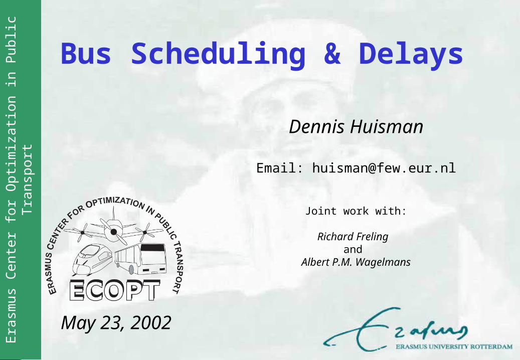
Contents
• Introduction
• Static versus Dynamic Scheduling
• Dynamic Vehicle Scheduling:– single-depot– multiple-depot
• Computational Experience
• Conclusions and Future Research

3
Era
smus
Ce
nte
r fo
r O
ptim
iza
tion
in P
ubl
ic T
rans
por
t
Introduction
T rip s
B lo cks a n d T a sks
C re w D u ties
C re w R o s te rsC re w R o s te ring
C re w S ch ed u ling
V e h ic le S ch e du ling
T im e T a b ling
lin e s + fre q ue n c ies
static
dynamic
4
Era
smus
Ce
nte
r fo
r O
ptim
iza
tion
in P
ubl
ic T
rans
por
t
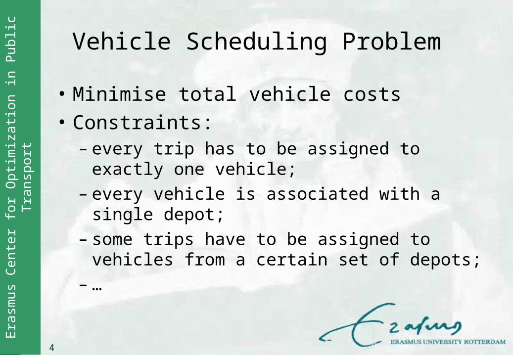
Vehicle Scheduling Problem
• Minimise total vehicle costs
• Constraints:– every trip has to be assigned to exactly one vehicle;– every vehicle is associated with a single depot;– some trips have to be assigned to vehicles from a
certain set of depots;– …
5
Era
smus
Ce
nte
r fo
r O
ptim
iza
tion
in P
ubl
ic T
rans
por
t
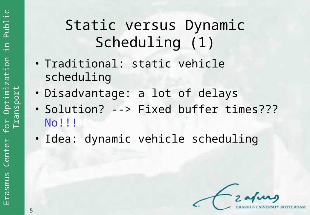
Static versus Dynamic Scheduling (1)
• Traditional: static vehicle scheduling• Disadvantage: a lot of delays• Solution? --> Fixed buffer times??? No!!!• Idea: dynamic vehicle scheduling
6
Era
smus
Ce
nte
r fo
r O
ptim
iza
tion
in P
ubl
ic T
rans
por
t
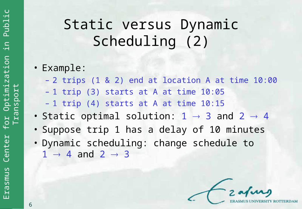
Static versus Dynamic Scheduling (2)
• Example:– 2 trips (1 & 2) end at location A at time 10:00– 1 trip (3) starts at A at time 10:05– 1 trip (4) starts at A at time 10:15
• Static optimal solution: 1 3 and 2 4• Suppose trip 1 has a delay of 10 minutes• Dynamic scheduling: change schedule to
1 4 and 2 3
7
Era
smus
Ce
nte
r fo
r O
ptim
iza
tion
in P
ubl
ic T
rans
por
t
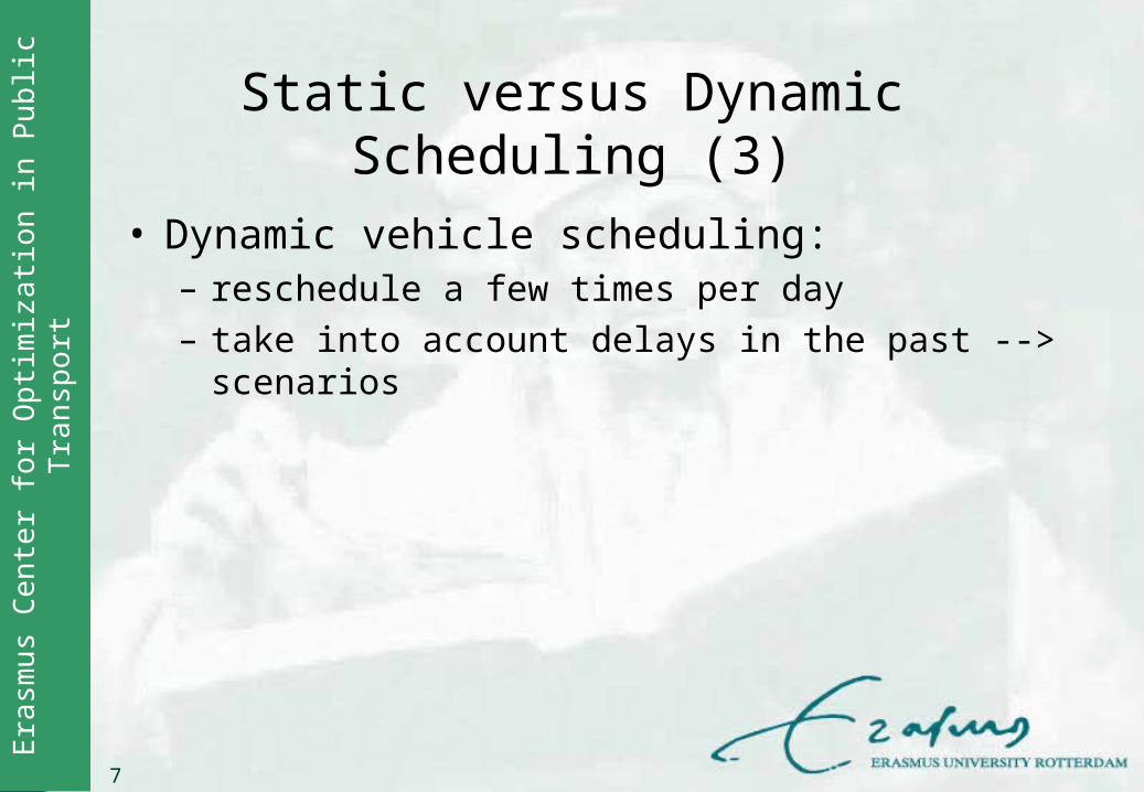
Static versus Dynamic Scheduling (3)
• Dynamic vehicle scheduling:– reschedule a few times per day– take into account delays in the past --> scenarios
8
Era
smus
Ce
nte
r fo
r O
ptim
iza
tion
in P
ubl
ic T
rans
por
t
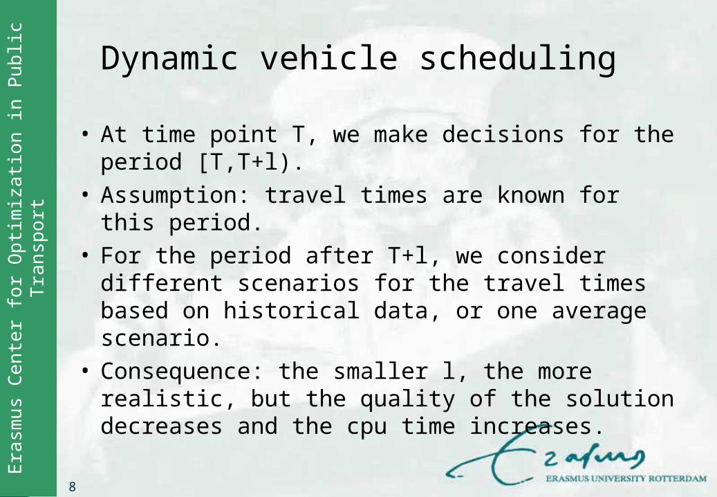
Dynamic vehicle scheduling
• At time point T, we make decisions for the period [T,T+l).
• Assumption: travel times are known for this period.
• For the period after T+l, we consider different scenarios for the travel times based on historical data, or one average scenario.
• Consequence: the smaller l, the more realistic, but the quality of the solution decreases and the cpu time increases.
9
Era
smus
Ce
nte
r fo
r O
ptim
iza
tion
in P
ubl
ic T
rans
por
t
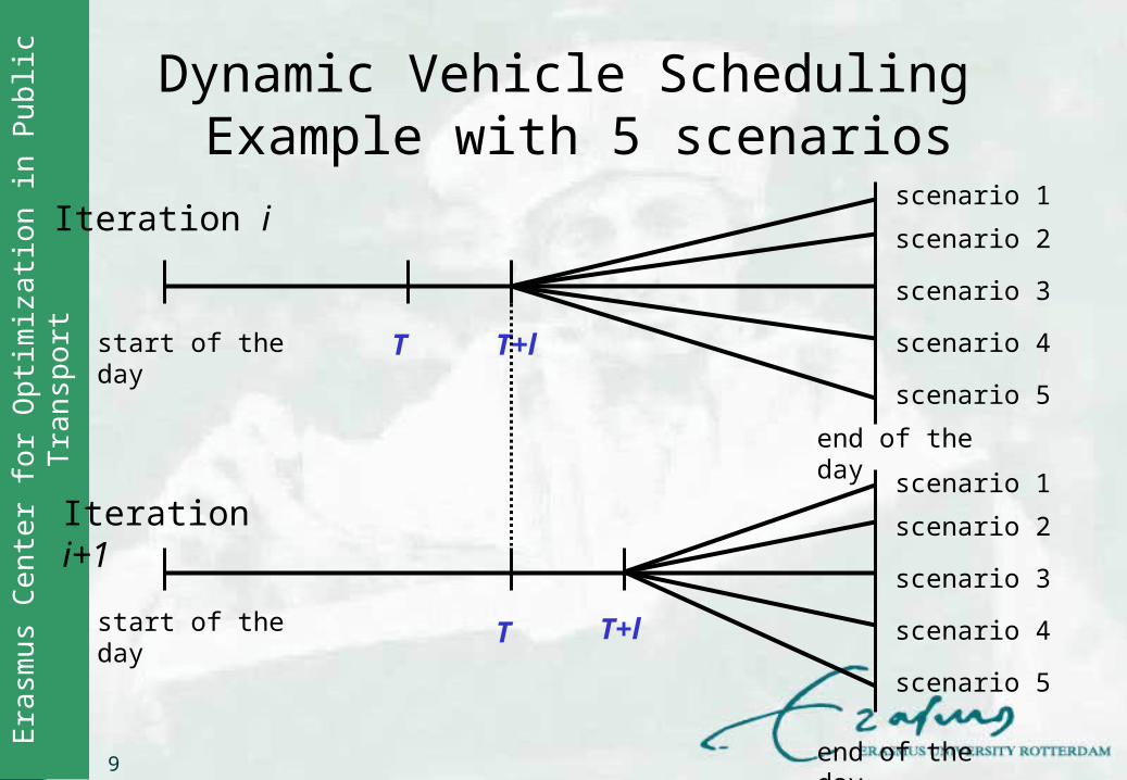
T T+l
end of the day
start of the day
scenario 1
scenario 2
scenario 5
scenario 3
scenario 4
Iteration i
end of the day
T
scenario 1
scenario 2
scenario 5
scenario 3
scenario 4start of the day T+l
Iteration i+1
Dynamic Vehicle Scheduling Example with 5 scenarios
10
Era
smus
Ce
nte
r fo
r O
ptim
iza
tion
in P
ubl
ic T
rans
por
t
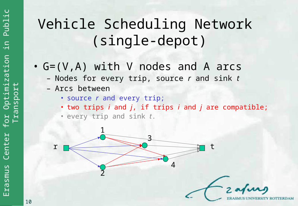
Vehicle Scheduling Network (single-depot)
• G=(V,A) with V nodes and A arcs – Nodes for every trip, source r and sink t– Arcs between
• source r and every trip;• two trips i and j, if trips i and j are compatible; • every trip and sink t.
2
r t
13
4
11
Era
smus
Ce
nte
r fo
r O
ptim
iza
tion
in P
ubl
ic T
rans
por
t
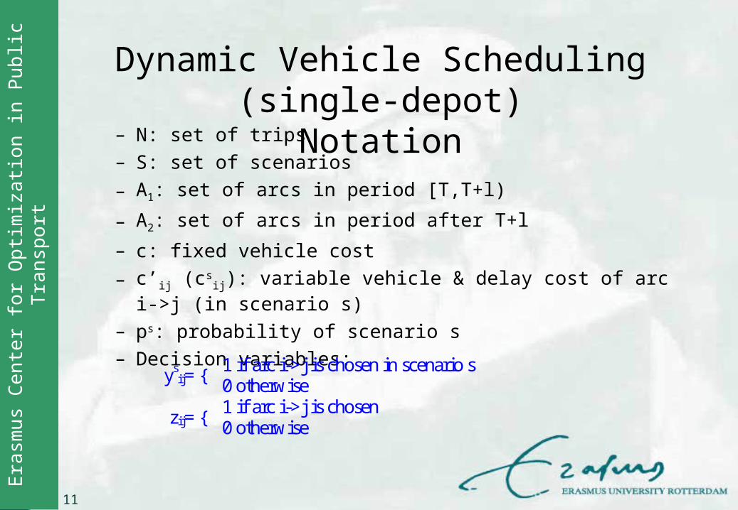
Dynamic Vehicle Scheduling (single-depot)Notation
– N: set of trips– S: set of scenarios
– A1: set of arcs in period [T,T+l)
– A2: set of arcs in period after T+l
– c: fixed vehicle cost
– c’ij (csij): variable vehicle & delay cost of arc i->j (in scenario s)
– ps: probability of scenario s– Decision variables:
1 if arc i->j is chosen in scenario s ys
ij= { 0 otherwise 1 if arc i->j is chosen
zij= { 0 otherwise
12
Era
smus
Ce
nte
r fo
r O
ptim
iza
tion
in P
ubl
ic T
rans
por
t
Assumption (1)
• Special cost structure:– fixed costs for every vehicle;– variable costs per time unit that a vehicle is without
passengers outside the depot.
13
Era
smus
Ce
nte
r fo
r O
ptim
iza
tion
in P
ubl
ic T
rans
por
t
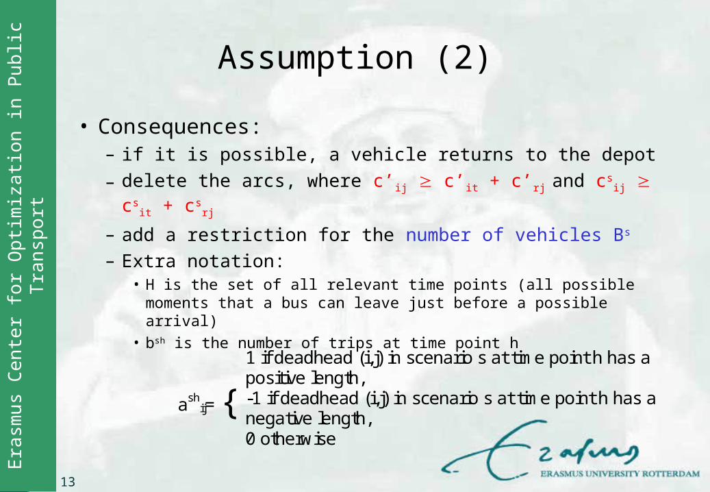
Assumption (2)
• Consequences: – if it is possible, a vehicle returns to the depot
– delete the arcs, where c’ij c’it + c’rj and csij cs
it + csrj
– add a restriction for the number of vehicles Bs
– Extra notation:• H is the set of all relevant time points (all possible moments
that a bus can leave just before a possible arrival)• bsh is the number of trips at time point h
1 if deadhead (i,j) in scenario s at time point h has a positive length, -1 if deadhead (i,j) in scenario s at time point h has a negative length,
ashij= {
0 otherwise
14
Era
smus
Ce
nte
r fo
r O
ptim
iza
tion
in P
ubl
ic T
rans
por
t
(6)Aj)(i,S,s {0,1}y
(5)Aj)(i,{0,1}z
(4)HhS,sbyazaB
(3)NjS,s1yz
(2)NiS,s1yz
(1)ycpzcBpcmin
2sij
1ij
Aj)(i, Aj)(i,
shsij
shijij
shij
s
}Aj)(i,:{i }Aj)(i,:{i
sijij
}Aj)(i,:{j }Aj)(i,:{j
sijij
Aj)(i,
sij
sij
Ss
s
Aj)(i,ij
'ij
Ss
ss
1 2
1 2
1 2
21
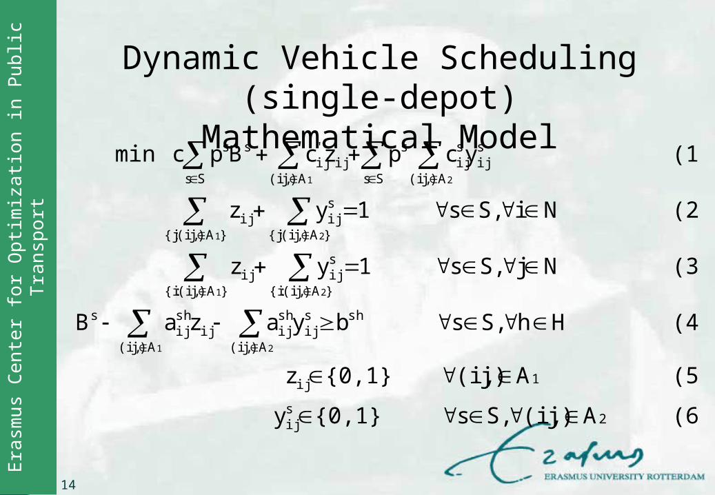
Dynamic Vehicle Scheduling (single-depot)Mathematical Model
15
Era
smus
Ce
nte
r fo
r O
ptim
iza
tion
in P
ubl
ic T
rans
por
t
Dynamic Vehicle Scheduling (multiple-depot)
• Size of the problem is very large• Cluster-Reschedule Heuristic:
– cluster the trips via the static MDVSP– reschedule per depot via the dynamic SDVSP
• Lagrangean Relaxation for computing lower bounds
16
Era
smus
Ce
nte
r fo
r O
ptim
iza
tion
in P
ubl
ic T
rans
por
t
Data (1)
• Data from Connexxion• 1104 trips and 4 depots• Rotterdam, Utrecht and Dordrecht• Average depot group size: 1.71
17
Era
smus
Ce
nte
r fo
r O
ptim
iza
tion
in P
ubl
ic T
rans
por
t
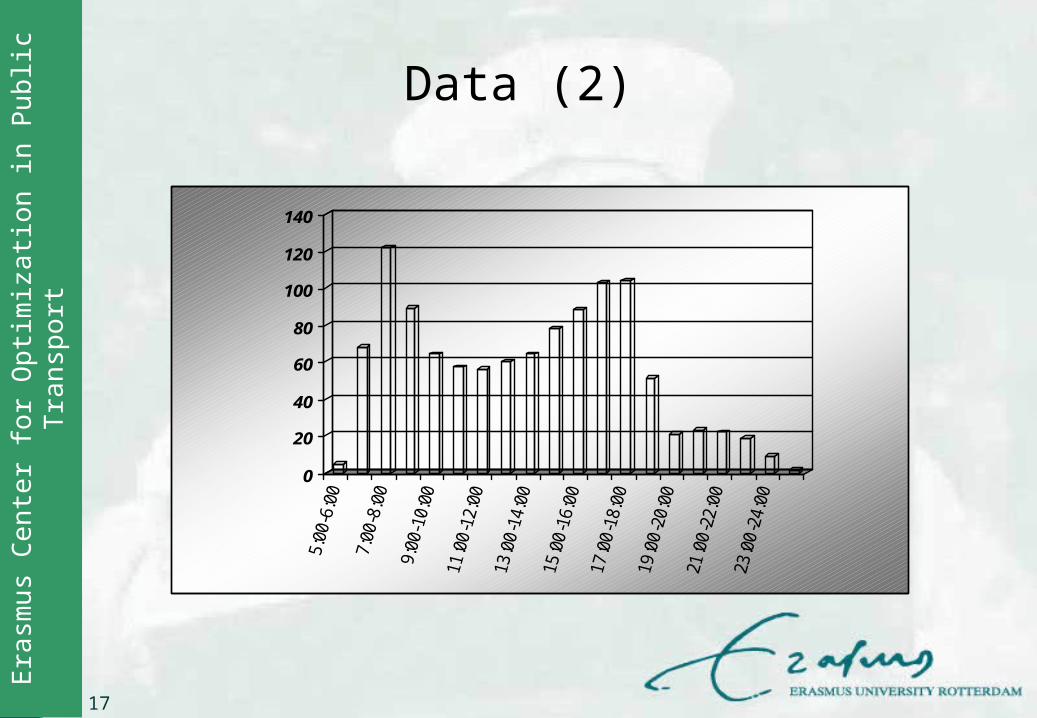
Data (2)
0
20
40
60
80
100
120
140
18
Era
smus
Ce
nte
r fo
r O
ptim
iza
tion
in P
ubl
ic T
rans
por
t
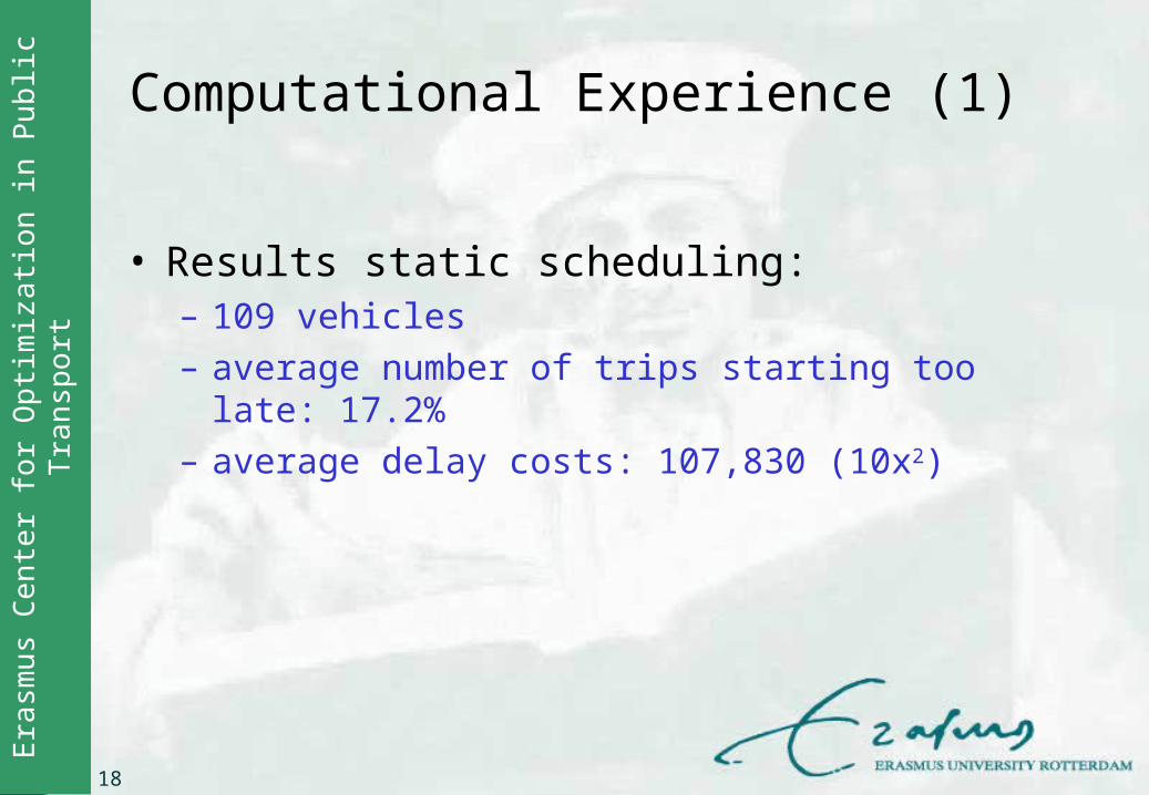
Computational Experience (1)
• Results static scheduling:– 109 vehicles– average number of trips starting too late: 17.2%– average delay costs: 107,830 (10x2)
19
Era
smus
Ce
nte
r fo
r O
ptim
iza
tion
in P
ubl
ic T
rans
por
t
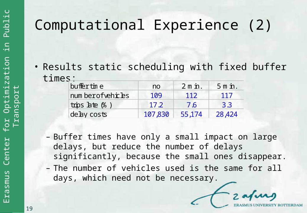
Computational Experience (2)
• Results static scheduling with fixed buffer times:
– Buffer times have only a small impact on large delays, but reduce the number of delays significantly, because the small ones disappear.
– The number of vehicles used is the same for all days, which need not be necessary.
buffer time no 2 min. 5 min.number of vehicles 109 112 117trips late (%) 17.2 7.6 3.3delay costs 107,830 55,174 28,424
20
Era
smus
Ce
nte
r fo
r O
ptim
iza
tion
in P
ubl
ic T
rans
por
t
Computational Experience (3)
• Dynamic scheduling:– fixed cost per delay;– cost for a delay is equal to the fixed cost per bus;– 9 scenarios (I) or 1 average scenario (II);– different values of l: 1, 5, 10, 15, 30, 60 and 120
minutes.
21
Era
smus
Ce
nte
r fo
r O
ptim
iza
tion
in P
ubl
ic T
rans
por
t
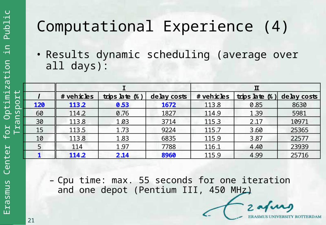
Computational Experience (4)
• Results dynamic scheduling (average over all days):
– Cpu time: max. 55 seconds for one iteration and one depot (Pentium III, 450 MHz)
l # vehicles trips late (%) delay costs # vehicles trips late (%) delay costs120 113.2 0.53 1672 113.8 0.85 863060 114.2 0.76 1827 114.9 1.39 598130 113.8 1.03 3714 115.3 2.17 1097115 113.5 1.73 9224 115.7 3.60 2536510 113.8 1.83 6835 115.9 3.87 225775 114 1.97 7788 116.1 4.40 239391 114.2 2.14 8960 115.9 4.99 25716
I II
22
Era
smus
Ce
nte
r fo
r O
ptim
iza
tion
in P
ubl
ic T
rans
por
t
Computational Experience (5)
• Lower bound:– gap between the cluster-reschedule heuristic and the
lower bound is in the first iteration about 3.5% (I) and 5.7% (II)
• Perfect information:– optimal: 110.6 vehicles– heuristic: 114.5 vehicles
• Sensitivity analysis:– small mistakes in the estimated travel times have a
small influence on the quality of the solution
23
Era
smus
Ce
nte
r fo
r O
ptim
iza
tion
in P
ubl
ic T
rans
por
t
Conclusions and Future Research
• An optimal solution for the static vehicle scheduling may lead to a lot of delays.
• Dynamic vehicle scheduling performs better in both the number of vehicles & the number of trips starting late than static vehicle scheduling with fixed buffer times.
• Future: – integration with crew scheduling.

24
Era
smus
Ce
nte
r fo
r O
ptim
iza
tion
in P
ubl
ic T
rans
por
t
25
Era
smus
Ce
nte
r fo
r O
ptim
iza
tion
in P
ubl
ic T
rans
por
t


![SCYCLE OPERATING UNIT POM, WEEE Generated & Flows in various EU Countries Tallinn, October 1, 2015 Jaco Huisman – Huisman [at] unu.edu](https://img.pdfslide.us/doc/110x75/5697bf8c1a28abf838c8bf7e/scycle-operating-unit-pom-weee-generated-flows-in-various-eu-countries-tallinn.jpg)