Equivariant Matlis and the local duality

Mitsuyasu Hashimoto and Masahiro Ohtani

Graduate School of Mathematics, Nagoya UniversityChikusa-ku, Nagoya 464–8602 JAPAN

hasimoto@math.nagoya-u.ac.jp m05011w@math.nagoya-u.ac.jp

Abstract

Generalizing the known results on graded rings and modules, weformulate and prove the equivariant version of the local duality onschemes with a group action. We also prove an equivariant analogueof Matlis duality.

1. Introduction

This paper is a continuation of [9], and study equivariant local cohomology.In this paper, utilizing an equivariant dualizing complex, we define the G-sheaf of matlis, an equivariant analogue of the injective hull of the residuefield of a local ring. Using this, we formulate and prove Matlis and the localduality under equivariant settings.

Let R be a Gorenstein local ring, T = R[x1, . . . , xs] be the graded poly-nomial ring with ri := deg xi positive, I a homogeneous ideal of height h,and A := T/I. Assume that A is Cohen–Macaulay of dimension d. SetωT := T (−r), where r =

∑i ri, and (−r) denotes the shift of degree. Set

ωA := ExthT (A,ωT ). For a graded A-module M , set M∨ :=⊕

i∈ZM†−i,

where (?)† = HomR(?, ER), where ER is the injective hull of the residuefield of R. Note that M∨ is a graded A-module again. Note also that∗HomA(M,A∨) ∼= M∨ (see for the notation ∗Hom, [1, page 33]).

For a finite graded A-module M , we have an isomorphism of graded A-modules

H iM(M) ∼= Extd−iA (M,ωA)∨,

cf. [1, Theorem 3.6.19], see also Corollary 5.5.

1

The main purpose of this paper is to generalize this graded version oflocal duality to more general equivariant local duality. Note that a gradedmodule over a Z-graded ring is nothing but an equivariant module underthe action of Gm = GL1, see [6, (II.1.2)]. On the way, we prove some basicproperties on equivariant local cohomology.

In this introduction, let S be a noetherian scheme, G a flat S-groupscheme of finite type, and X a noetherian G-scheme. In order to establish ananalogy of the local duality on X, we need to define an equivariant analogueof a local ring or a local scheme. This is done in [9], and it is a G-localG-scheme. So let X be a G-local G-scheme. That is to say, X has a uniqueminimal nonempty G-stable closed G-subscheme, say Y . Next, we need tohave an equivariant analogue of local cohomology. This is the main subjectof [9]. Finally, we need to have an analogy of the Matlis duality. In otherwords, we need to have an analogue of the injective hull of the residue fieldof a local ring. The authors do not know how to define it quite generally.However, if X has a G-equivariant dualizing complex (see for the definition,[7, chapter 31]) IX , then we can define it as the unique nonzero cohomologygroup of RΓY (IX). We call this sheaf the G-sheaf of Matlis. Thus we can for-mulate the equivariant local duality. The proof depends on the isomorphismH, see below.

Many ideas used in this paper have already appeared in the theory ofgraded rings [3], [4], [1], [10]. If H is a finitely generated abelian group, thenletting G = SpecZH, where ZH is the group algebra of H over Z, an H-graded algebra is nothing but a G-algebra, and for a G-algebra A, a gradedA-module is nothing but a (G,A)-module. However, we need to point outthat for a general G and a G-local G-algebra (A,M) with the G-dualizingcomplex I, the global section of the G-sheaf of Matlis EA is not necessarilyinjective as a (G,A)-module, see Example 5.7. In particular, EA is not theinjective hull of A/M in the category of (G,A)-modules.

Using the G-sheaf of Matlis, we can prove a weak version of the Matlisduality, too. It is a duality from the category of coherent (G,OX)-modulesof finite length to itself, see Theorem 4.17. Note that a better Matlis dualityexists over a complete local ring. It is a duality from the category of noethe-rian modules to the category of artinian modules ([1, Theorem 3.2.13]). Theauthors do not know a good analogue of a complete local ring, and thuscannot give an equivariant Matlis duality between noetherian quasi-coherent(G,OX)-modules and artinian modules in general. However, there is an ex-ample of graded case of that kind of duality, see Remark 5.6.

2

Section 2 is preliminaries. We give some basic properties of the dualitymap in a closed category. We also give some sufficient conditions to guaran-tee that injective objects in the category Qch(G,X) is acyclic with respectto some cohomological functors. We also prove a generalization of the flatbase change ([9, Theorem 6.10]), see Lemma 2.14. We also describe the lo-cal cohomology over a diagram of schemes using the inductive limit of Extgroups, as in the single-scheme case.

Section 3 treats the map H. For a small category I, an Iop-diagram ofschemes X, an open subdiagram of schemes U of X, and an open subdiagramof schemes V of U , there is a natural map

H : ΓU,V HomOX (M,N )→ HomOX (M,ΓU,V N )

for M,N ∈ Mod(X). There is an obvious derived version of it, and H

is often an isomorphism (see Lemma 3.16 and Theorem 3.26). This is thekey to the proof of the equivariant version of the local duality. In orderto establish the existence and some basic properties of H, we need to provevarious commutativity of diagrams. To do this, we utilize the basics on closedcategories as in [7, chapter 1].

In section 4, we formulate and prove the equivariant analogues of Matlisand the local duality. We start with Matijevic–Roberts type theorem forG-local G-schemes, and prove an equivariant version of Nakayama’s lemma,which is well-known for affine case.

In section 5, we give an example of the graded case. Note that in somecases, Matlis duality can be in more general form than the version describedin section 4, see Remark 5.6.

2. Preliminaries

(2.1) We use the notation and terminology of [7], [9], and [8] freely.

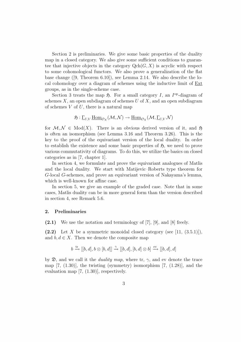
(2.2) Let X be a symmetric monoidal closed category (see [11, (3.5.1)]),and b, d ∈ X. Then we denote the composite map

btr−→ [[b, d], b⊗ [b, d]]

γ−→ [[b, d], [b, d]⊗ b] ev−→ [[b, d], d]

by D, and we call it the duality map, where tr, γ, and ev denote the tracemap [7, (1.30)], the twisting (symmetry) isomorphism [7, (1.28)], and theevaluation map [7, (1.30)], respectively.

3

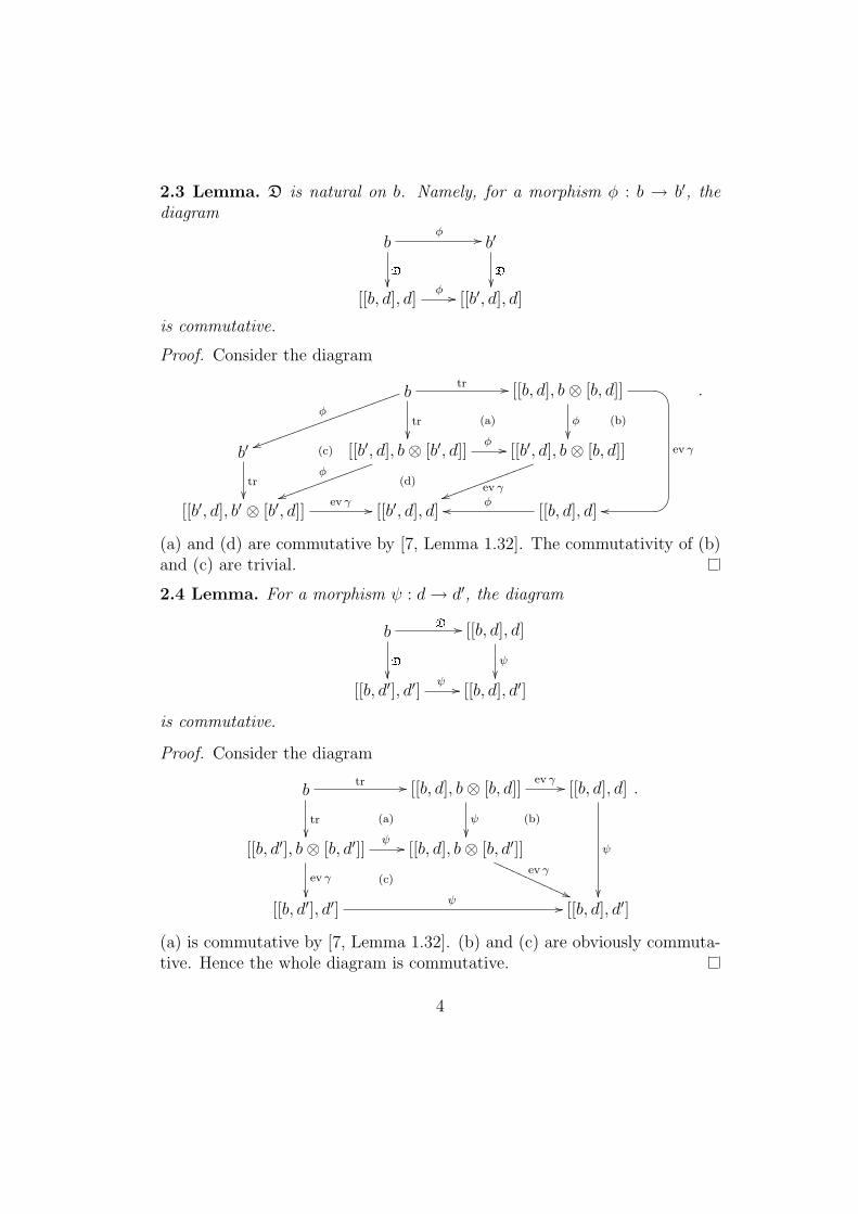
2.3 Lemma. D is natural on b. Namely, for a morphism φ : b → b′, thediagram

bφ //

D��

b′

D��

[[b, d], d]φ // [[b′, d], d]

is commutative.

Proof. Consider the diagram

bφ

uukkkkkkkkkkkkkkkkkkkkkk

tr��

tr //

(a)

(c)

[[b, d], b⊗ [b, d]]

φ

��(b)

ED

BC

ev γ

oo

b′

tr��

[[b′, d], b⊗ [b′, d]]φ

uukkkkkkkkkkkkkk

φ //

(d)

[[b′, d], b⊗ [b, d]]

ev γuukkkkkkkkkkkkkk

[[b′, d], b′ ⊗ [b′, d]]ev γ // [[b′, d], d] [[b, d], d]

φoo

.

(a) and (d) are commutative by [7, Lemma 1.32]. The commutativity of (b)and (c) are trivial.

2.4 Lemma. For a morphism ψ : d→ d′, the diagram

bD //

D��

[[b, d], d]

ψ

��[[b, d′], d′]

ψ // [[b, d], d′]

is commutative.

Proof. Consider the diagram

btr //

tr��

(a)

[[b, d], b⊗ [b, d]]

ψ

��

ev γ //

(b)

[[b, d], d]

ψ

��

[[b, d′], b⊗ [b, d′]]ψ //

ev γ

��(c)

[[b, d], b⊗ [b, d′]]ev γ

((PPPPPPPPPPPP

[[b, d′], d′]ψ // [[b, d], d′]

.

(a) is commutative by [7, Lemma 1.32]. (b) and (c) are obviously commuta-tive. Hence the whole diagram is commutative.

4

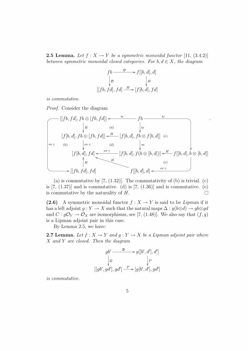
2.5 Lemma. Let f : X → Y be a symmetric monoidal functor [11, (3.4.2)]between symmetric monoidal closed categories. For b, d ∈ X, the diagram

fbD //

D��

f [[b, d], d]

H��

[[fb, fd], fd] H // [f [b, d], fd]

is commutative.

Proof. Consider the diagram

[[fb, fd], fb⊗ [fb, fd]]

H��

GF

@A

ev γ

//

(a)

fb

tr��

trooED

tr

��(b)

[f [b, d], fb⊗ [fb, fd]]

ev γ

��(d)

[f [b, d], fb⊗ f [b, d]]

m

��

(c)Hoo

[f [b, d], fd] [f [b, d], f(b⊗ [b, d])]ev γoo

(e)

f [[b, d], b⊗ [b, d]]Hoo

BCev γoo[[fb, fd], fd]

H

OO

f [[b, d], d]

HjjUUUUUUUUUUUUUUUUU

.

(a) is commutative by [7, (1.32)]. The commutativity of (b) is trivial. (c)is [7, (1.37)] and is commutative. (d) is [7, (1.36)] and is commutative. (e)is commutative by the naturality of H.

(2.6) A symmetric monoidal functor f : X → Y is said to be Lipman if ithas a left adjoint g : Y → X such that the natural maps ∆ : g(b⊗d)→ gb⊗gdand C : gOY → OX are isomorphisms, see [7, (1.48)]. We also say that (f, g)is a Lipman adjoint pair in this case.

By Lemma 2.5, we have:

2.7 Lemma. Let f : X → Y and g : Y → X be a Lipman adjoint pair whereX and Y are closed. Then the diagram

gb′ D //

D��

g[[b′, d′], d′]

P��

[[gb′, gd′], gd′] P // [g[b′, d′], gd′]

is commutative.

5

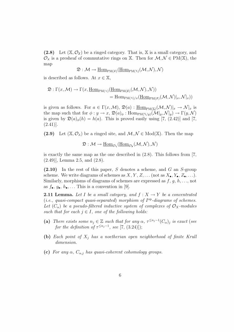
(2.8) Let (X,OX) be a ringed category. That is, X is a small category, andOX is a presheaf of commutative rings on X. Then for M,N ∈ PM(X), themap

D :M→ HomPM(X)(HomPM(X)(M,N ),N )

is described as follows. At x ∈ X,

D : Γ(x,M)→ Γ(x,HomPM(X)(HomPM(X)(M,N ),N ))

= HomPM(X)/x(HomPM(X)(M,N )|x,N|x))

is given as follows. For a ∈ Γ(x,M), D(a) : HomPM(X)(M,N )|x → N|x isthe map such that for φ : y → x, D(a)φ : HomPM(X/y)(M|y,N|y)→ Γ(y,N )is given by D(a)φ(h) = h(a). This is proved easily using [7, (2.42)] and [7,(2.41)].

(2.9) Let (X,OX) be a ringed site, and M,N ∈ Mod(X). Then the map

D :M→ HomOX(HomOX(M,N ),N )

is exactly the same map as the one described in (2.8). This follows from [7,(2.49)], Lemma 2.5, and (2.8).

(2.10) In the rest of this paper, S denotes a scheme, and G an S-groupscheme. We write diagrams of schemes as X, Y , Z, . . . (not as X•, Y•, Z•, . . .).Similarly, morphisms of diagrams of schemes are expressed as f , g, h, . . ., notas f•, g•, h•, . . . This is a convention in [9].

2.11 Lemma. Let I be a small category, and f : X → Y be a concentrated(i.e., quasi-compact quasi-separated) morphism of Iop-diagrams of schemes.Let (Cα) be a pseudo-filtered inductive system of complexes of OX-modulessuch that for each j ∈ I, one of the following holds:

(a) There exists some nj ∈ Z such that for any α, τ≤nj−1(Cα)j is exact (seefor the definition of τ≤nj−1, see [7, (3.24)]);

(b) Each point of Xj has a noetherian open neighborhood of finite Krulldimension.

(c) For any α, Cα,j has quasi-coherent cohomology groups.

6

Set C = lim−→Cα. Then the canonical map

(1) lim−→Rif∗Cα → Rif∗C

is an isomorphism for i ∈ Z. If, moreover, each Cα is f∗-acyclic, then C isf∗-acyclic.

Proof. In view of [7, Example 8.23, 2], it is easy to see that it suffices toshow that

lim−→Ri(fj)∗Cα,j → Ri(fj)∗Cj

is an isomorphism for each j, to prove that (1) is an isomorphism. This is(3.9.3.1) and (3.9.3.2) of [11].

To prove the last assertion, it suffices to show that each Cj is (fj)∗-acyclic.This is [11, (3.9.3.4)].

2.12 Corollary. Let f : X → Y be as in Lemma 2.11. Let C be a complex ofOX-modules such that each term of C is locally quasi-coherent and f∗-acyclic.Then C is f∗-acyclic.

Proof. Similar to [11, (3.9.3.5)].

2.13 Lemma. Let X and Y be S-groupoid (see for the definition, [7, (12.1)])and f : X → Y a morphism (in the category P(∆M , Sch/S), see for thenotation, [7, Glossary]). Assume that f is cartesian, Y has affine arrows,and assume one of the following:

(a) X0 is noetherian;

(b) Y0 and f0 are quasi-compact separated.

Then

(i) f is concentrated and X0 is concentrated.

(ii) A K-injective complex I in K(Qch(X)) is f∗-acyclic.

(iii) The canonical maps

FY ◦RfQch∗ ∼= R(FY ◦ fQch

∗ ) ∼= R(f∗ ◦ FX)→ Rf∗ ◦ FXare all isomorphisms, where FY : D(Qch(Y )) → D(Y ) and FX :D(Qch(X)) → D(X) are triangulated functors induced by inclusions,and fQch

∗ : Qch(X) → Qch(Y ) is the restriction of f∗ : Mod(X) →Mod(Y ), see [7, Lemma 7.14].

7

Proof. (i) In either case, f0 is concentrated. Since f is cartesian, each fi(i = 0, 1, 2) is obtained as a base change of f0, and hence is concentrated. Itis easy to see that X0 is concentrated in either case.

(ii) As f is concentrated cartesian, fQch∗ is well-defined [7, Lemma 7.14].

Since X0 is concentrated and X has affine arrows, Qch(X) is Grothendieckby [7, Lemma 12.8]. So I has a strictly injective resolution (that is, a K-injective resolution each of whose term is injective) J [2, Proposition 3.2]. Asthe mapping cone of I→ J is null-homotopic, replacing I by J, we may assumethat I is strictly injective. By Corollary 2.12, it suffices to show that eachterm of I is f∗-acyclic. So we may assume that I is a single injective objectof Qch(X). Let I0 → K be a monomorphism with K an injective object ofQch(X0). This is possible, since Qch(X0) is Grothendieck [7, Corollary 11.7].Note that the restriction (?)0 : Qch(X) → Qch(X0) has the right adjoint(d0)Qch

∗ ◦ A, see [7, Lemma 12.11]. As (?)0 is faithful exact, the composite

I→ (d0)Qch∗ AI0 → (d0)Qch

∗ AK

is a monomorphism into an injective object. This must split, and hence wemay further assume that I = (d0)Qch

∗ AK.By restriction, it suffices to show that Rj(fi)∗Ii = 0 for i = 0, 1, 2 and

j > 0. Since (?)iA ∼= r0(i + 1)∗ (see for the notation, [7, (9.1)]) and (d0) isaffine,

Rj(fi)∗Ii ∼= Rj(fi)∗d0(i+ 1)∗r0(i+ 1)∗K ∼= Rj(fi ◦ d0(i+ 1))∗r0(i+ 1)∗K

= Rj(d0(i+ 1) ◦ fi+1)∗r0(i+ 1)∗K ∼= d0(i+ 1)∗Rj(fi+1)∗r0(i+ 1)∗K∼= d0(i+ 1)∗r0(i+ 1)∗Rj(f0)∗K = 0

for j > 0 by [7, Lemma 14.6, 1] and its proof. This is what we wanted toprove.

(iii) Follows immediately from (ii).The following is a generalization of [9, Theorem 6.10].

2.14 Lemma. Let I be a small category, h : X ′ → X a flat morphism ofIop-diagrams of schemes. Let f : U ↪→ X be an open subdiagram of schemes,and g : V ↪→ U be an open subdiagram of schemes. Assume that f and gare quasi-compact. Let f ′ : U ′ ↪→ X ′ and g′ : V ′ ↪→ U ′ be the base changeof f and g, respectively. Then δ̄ : h∗RΓU,V → RΓU ′,V ′ h

∗ in [9, (6.1)] is anisomorphism between functors from DLqc(X) to DLqc(X

′).

8

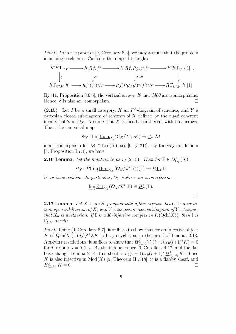
Proof. As in the proof of [9, Corollary 6.3], we may assume that the problemis on single schemes. Consider the map of triangles

h∗RΓU,V //

δ̄��

h∗Rf∗f ∗ //

d�

h∗Rf∗Rg∗g∗f ∗ //

ddθθ��

h∗RΓU,V [1]

��RΓU ′,V ′ h

∗ // Rf ′∗(f′)∗h∗ // Rf ′∗Rg

′∗(g′)∗(f ′)∗h∗ // RΓU ′,V ′ h

∗[1]

.

By [11, Proposition 3.9.5], the vertical arrows dθ and ddθθ are isomorphisms.Hence, δ̄ is also an isomorphism.

(2.15) Let I be a small category, X an Iop-diagram of schemes, and Y acartesian closed subdiagram of schemes of X defined by the quasi-coherentideal sheaf I of OX . Assume that X is locally noetherian with flat arrows.Then, the canonical map

ΦY : lim−→HomOX (OX/In,M)→ ΓY Mis an isomorphism for M ∈ Lqc(X), see [9, (3.21)]. By the way-out lemma[5, Proposition I.7.1], we have

2.16 Lemma. Let the notation be as in (2.15). Then for F ∈ D+Lqc(X),

ΦY : R(lim−→HomOX (OX/In, ?))(F)→ RΓY F

is an isomorphism. In particular, ΦY induces an isomorphism

lim−→ExtiOX (OX/In,F) ∼= H iY (F).

2.17 Lemma. Let X be an S-groupoid with affine arrows. Let U be a carte-sian open subdiagram of X, and V a cartesian open subdiagram of Y . Assumethat X0 is noetherian. If I is a K-injective complex in K(Qch(X)), then I isΓU,V -acyclic.

Proof. Using [9, Corollary 6.7], it suffices to show that for an injective objectK of Qch(X0), (d0)Qch

∗ AK is ΓU,V -acyclic, as in the proof of Lemma 2.13.

Applying restrictions, it suffices to show that HjUi,Vi

(d0(i+1)∗r0(i+1)∗K) = 0for j > 0 and i = 0, 1, 2. By the independence [9, Corollary 4.17] and the flatbase change Lemma 2.14, this sheaf is d0(i + 1)∗r0(i + 1)∗Hj

U0,V0K. Since

K is also injective in Mod(X) [5, Theorem II.7.18], it is a flabby sheaf, andHjU0,V0

K = 0.

9

(2.18) A G-scheme X (i.e., an S-scheme with a left G-action) is said to bestandard if X is noetherian, and the second projection p2 : G × X → X isflat of finite type.

Let X be a standard G-scheme. We denote the category of quasi-coherent(resp. coherent) (G,OX)-modules by Qch(G,X) (resp. Coh(G,X)). Notethat the sheaf theory discussed in [7, chapters 29–31] and [9], where weassume that G is flat of finite type over S, still works under our weakerassumption (p2 is flat of finite type). In particular, Qch(G,X) is a locallynoetherian category, and M∈ Qch(G,X) is a noetherian object if and onlyif M∈ Coh(G,X), see [7, Lemma 12.8].

(2.19) We say that a standard G-scheme X is G-artinian if there is no in-cidence relation between G-prime G-ideals (see for the definition, [8, (4.12)])of X.

2.20 Lemma. If X is G-artinian, then X is a disjoint union of finitely manyG-artinian G-local G-schemes.

Proof. Clearly, the set of all G-prime G-ideals SpecG(X) agrees with thefinite set MinG(OX), the set of minimal G-primes of 0. Thus there areonly finitely many G-prime G-ideals. For P ,Q ∈ SpecG(X) with P 6= Q,AssG(OX/(P +Q)) = ∅, since there is no G-prime G-ideal containing bothP and Q. Thus P +Q = OX . This shows that X =

∐P∈SpecG(X) V (P). As

each V (P) is clearly G-artinian G-local, we are done.

3. The map H

(3.1) Let f : X → Y be a symmetric monoidal functor between symmetricmonoidal closed categories, and g : Y → X its right adjoint. For b ∈ Y andd ∈ X, we denote the composite map

f [gb, d]H−→ [fgb, fd]

u−→ [b, fd]

by ϑ.

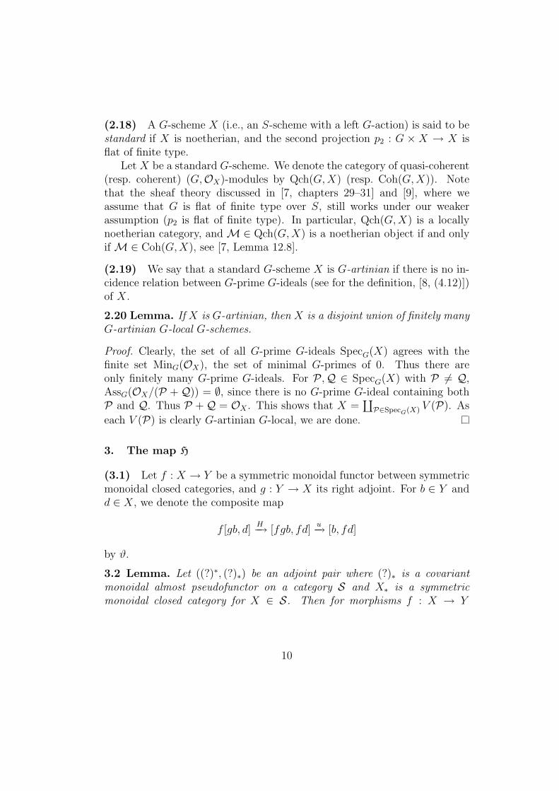
3.2 Lemma. Let ((?)∗, (?)∗) be an adjoint pair where (?)∗ is a covariantmonoidal almost pseudofunctor on a category S and X∗ is a symmetricmonoidal closed category for X ∈ S. Then for morphisms f : X → Y

10

and g : Y → Z of S and b, d ∈ Z∗, the diagram

(2) (gf)∗(b⊗ d) ∆ //

d−1

��

(gf)∗b⊗ (gf)∗d

d−1⊗d−1

��f ∗g∗(b⊗ d) ∆ // f ∗(g∗b⊗ g∗d) ∆ // f ∗g∗b⊗ f ∗g∗d

is commutative.

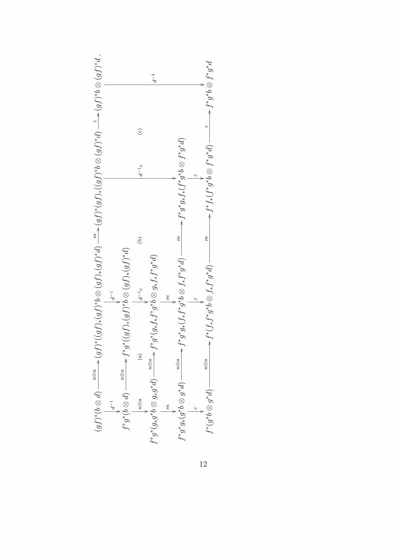
Proof. Consider the diagram

11

(gf

)∗(b⊗d)

u⊗u

//

d−

1

��

(gf

)∗((gf

) ∗(gf

)∗b⊗

(gf

) ∗(gf

)∗d)

m//

d−

1

��

(gf

)∗(gf

) ∗((gf

)∗b⊗

(gf

)∗d)

ε//

d−

1c

��

(gf

)∗b⊗

(gf

)∗d

d−

1

��

f∗ g∗ (b⊗d)

u⊗u

//

u⊗u

��(a

)f∗ g∗ (

(gf

) ∗(gf

)∗b⊗

(gf

) ∗(gf

)∗d)

d−

1c

��(b

)(c

)

f∗ g∗ (g ∗g∗ b⊗g ∗g∗ d

)u⊗u

//

m ��

f∗ g∗ (g ∗f ∗f∗ g∗ b⊗g ∗f ∗f∗ g∗ d

)

m ��f∗ g∗ g∗(g∗ b⊗g∗ d

)u⊗u

//

ε ��

f∗ g∗ g∗(f ∗f∗ g∗ b⊗f ∗f∗ g∗ d

)m

//

ε ��

f∗ g∗ g∗f∗(f∗ g∗ b⊗f∗ g∗ d

)

ε ��f∗ (g∗ b⊗g∗ d

)u⊗u

// f∗ (f ∗f∗ g∗ b⊗f ∗f∗ g∗ d

)m

// f∗ f∗(f∗ g∗ b⊗f∗ g∗ d

)ε

// f∗ g∗ b⊗f∗ g∗ d

.

12

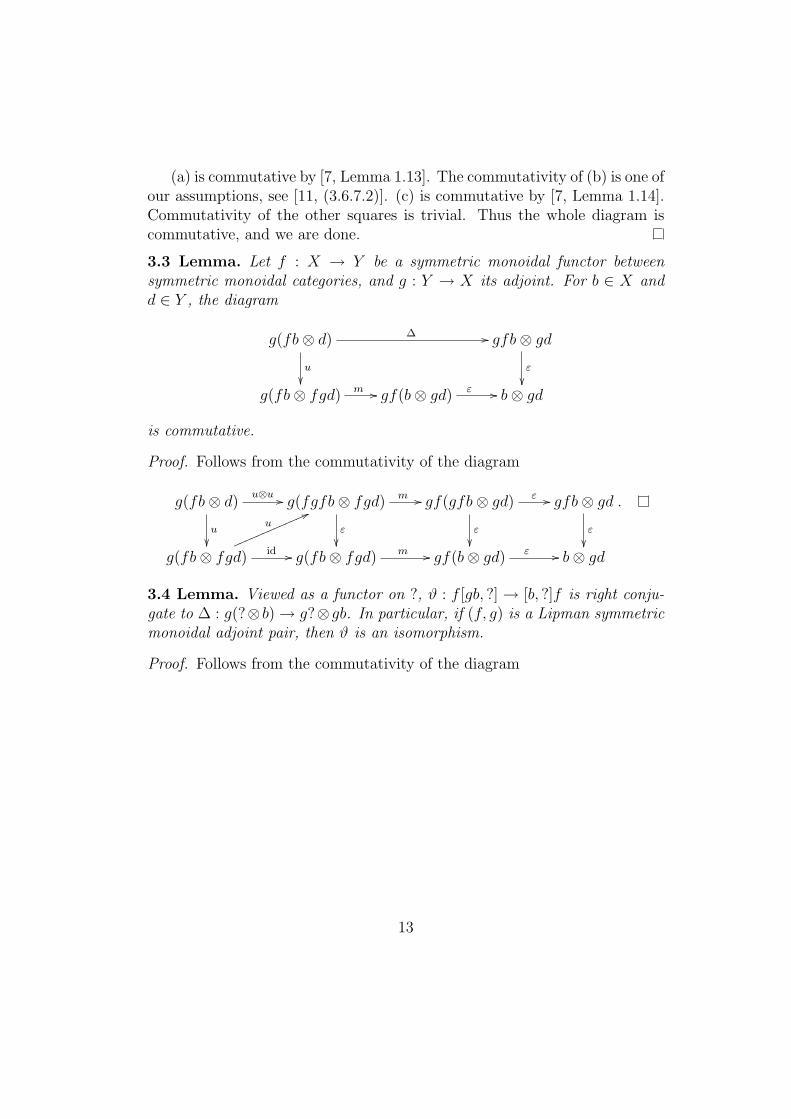
(a) is commutative by [7, Lemma 1.13]. The commutativity of (b) is one ofour assumptions, see [11, (3.6.7.2)]. (c) is commutative by [7, Lemma 1.14].Commutativity of the other squares is trivial. Thus the whole diagram iscommutative, and we are done.

3.3 Lemma. Let f : X → Y be a symmetric monoidal functor betweensymmetric monoidal categories, and g : Y → X its adjoint. For b ∈ X andd ∈ Y , the diagram

g(fb⊗ d) ∆ //

u

��

gfb⊗ gdε

��g(fb⊗ fgd) m // gf(b⊗ gd) ε // b⊗ gd

is commutative.

Proof. Follows from the commutativity of the diagram

g(fb⊗ d)u⊗u //

u

��

g(fgfb⊗ fgd) m //

ε

��

gf(gfb⊗ gd) ε //

ε

��

gfb⊗ gdε

��g(fb⊗ fgd)

u66mmmmmmmmmmmmm

id // g(fb⊗ fgd) m // gf(b⊗ gd) ε // b⊗ gd

.

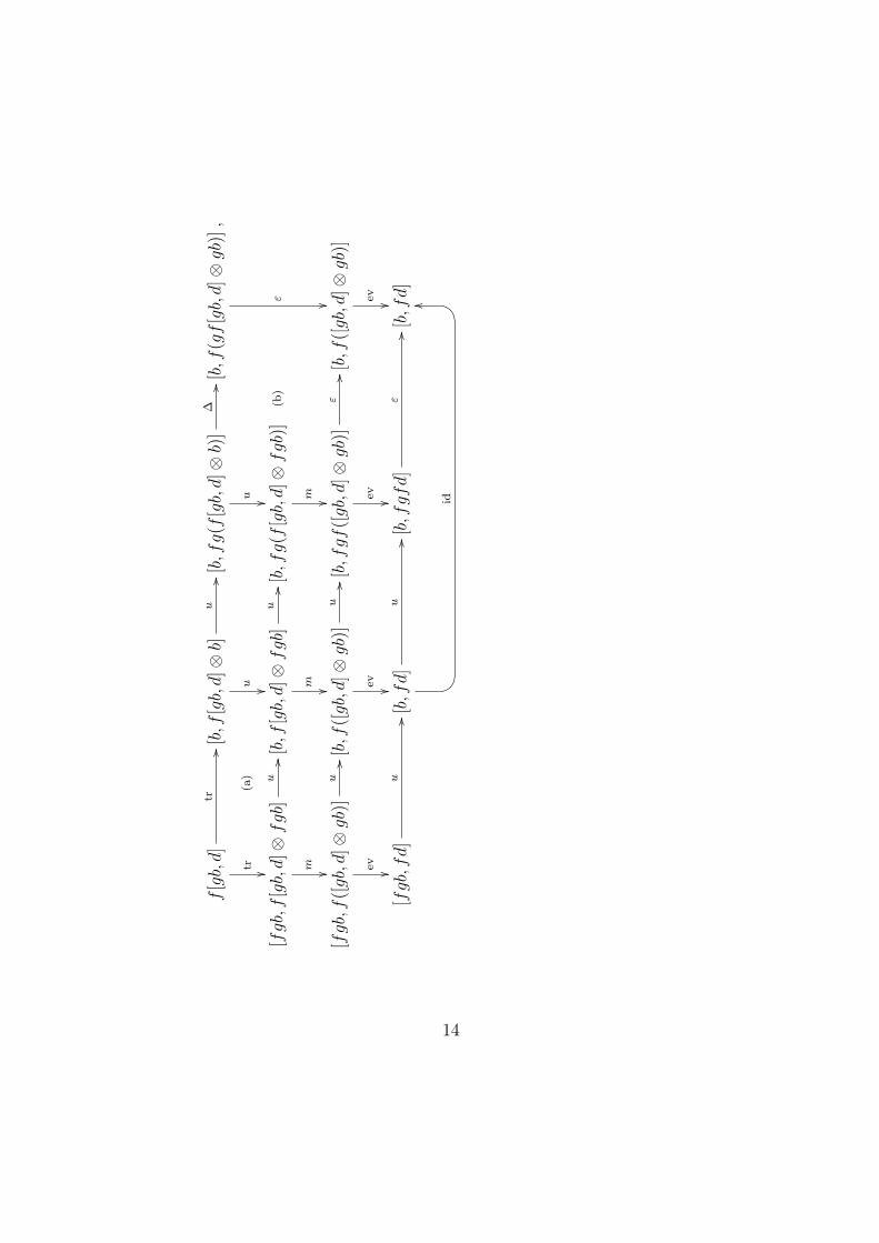
3.4 Lemma. Viewed as a functor on ?, ϑ : f [gb, ?]→ [b, ?]f is right conju-gate to ∆ : g(?⊗ b)→ g?⊗gb. In particular, if (f, g) is a Lipman symmetricmonoidal adjoint pair, then ϑ is an isomorphism.

Proof. Follows from the commutativity of the diagram

13

f[gb,d]

tr//

tr ��(a

)

[b,f

[gb,d]⊗

b]u

//

u ��

[b,fg(f

[gb,d]⊗

b)]

∆//

u ��

[b,f

(gf

[gb,d]⊗

gb)

]

ε ��

[fgb,f

[gb,d]⊗

fgb]

u//

m ��

[b,f

[gb,d]⊗

fgb]

u//

m ��

[b,fg(f

[gb,d]⊗

fgb)

]

m ��

(b)

[fgb,f

([gb,d]⊗

gb)

]u

//

ev ��

[b,f

([gb,d]⊗

gb)

]u

//

ev ��

[b,fgf

([gb,d]⊗

gb)

]ε

//

ev ��

[b,f

([gb,d]⊗

gb)

]

ev ��[fgb,fd]

u// [b,fd]

u//

@ABC

id

OO[b,fgfd]

ε// [b,fd]

,

14

where the commutativity of (a) and (b) follows from [7, (1.32)] andLemma 3.3, respectively.

Consider that the diagram (2) is that of functors on b (consider that d isfixed), and then take a conjugate diagram, we immediately have:

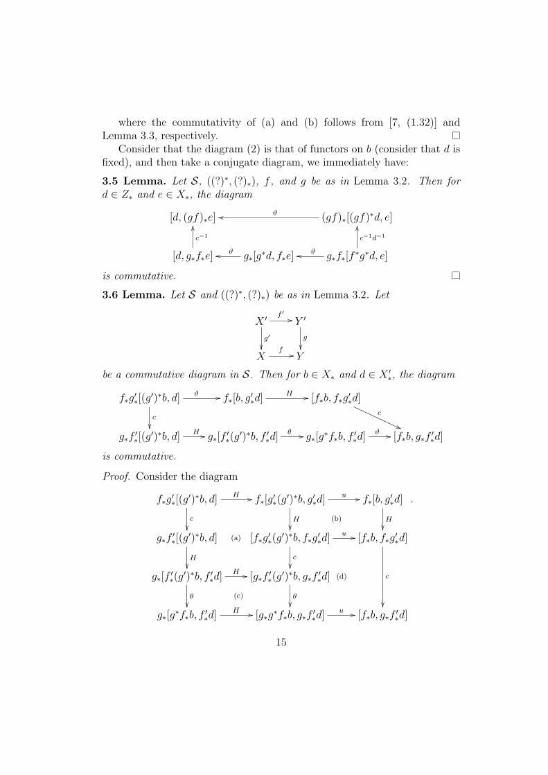
3.5 Lemma. Let S, ((?)∗, (?)∗), f , and g be as in Lemma 3.2. Then ford ∈ Z∗ and e ∈ X∗, the diagram

[d, (gf)∗e] (gf)∗[(gf)∗d, e]ϑoo

[d, g∗f∗e]

c−1

OO

g∗[g∗d, f∗e]ϑoo g∗f∗[f ∗g∗d, e]

ϑoo

c−1d−1

OO

is commutative.

3.6 Lemma. Let S and ((?)∗, (?)∗) be as in Lemma 3.2. Let

X ′f ′ //

g′��

Y ′

g

��X

f // Y

be a commutative diagram in S. Then for b ∈ X∗ and d ∈ X ′∗, the diagram

f∗g′∗[(g′)∗b, d] ϑ //

c

��

f∗[b, g′∗d] H // [f∗b, f∗g′∗d]c

((PPPPPPPPPPPP

g∗f ′∗[(g′)∗b, d] H // g∗[f ′∗(g

′)∗b, f ′∗d] θ // g∗[g∗f∗b, f ′∗d] ϑ // [f∗b, g∗f ′∗d]

is commutative.

Proof. Consider the diagram

f∗g′∗[(g′)∗b, d] H //

c

��

f∗[g′∗(g′)∗b, g′∗d] u //

H��

(b)

f∗[b, g′∗d]

H��

g∗f ′∗[(g′)∗b, d] (a)

H��

[f∗g′∗(g′)∗b, f∗g′∗d]

c

��

u // [f∗b, f∗g′∗d]

c

��

g∗[f ′∗(g′)∗b, f ′∗d]

(c)�

H // [g∗f ′∗(g′)∗b, g∗f ′∗d] (d)

�

g∗[g∗f∗b, f ′∗d] H // [g∗g∗f∗b, g∗f ′∗d] u // [f∗b, g∗f ′∗d]

.

15

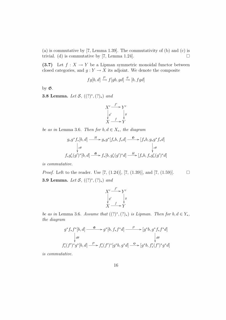
(a) is commutative by [7, Lemma 1.39]. The commutativity of (b) and (c) istrivial. (d) is commutative by [7, Lemma 1.24].

(3.7) Let f : X → Y be a Lipman symmetric monoidal functor betweenclosed categories, and g : Y → X its adjoint. We denote the composite

fg[b, d]P−→ f [gb, gd]

ϑ−→ [b, fgd]

by G.

3.8 Lemma. Let S, ((?)∗, (?)∗) and

X ′f ′ //

g′��

Y ′

g

��X

f // Y

be as in Lemma 3.6. Then for b, d ∈ X∗, the diagram

g∗g∗f∗[b, d] H //

c�

g∗g∗[f∗b, f∗d] G // [f∗b, g∗g∗f∗d]

c�

f∗g′∗(g′)∗[b, d] G // f∗[b, g′∗(g

′)∗d] H // [f∗b, f∗g′∗(g′)∗d]

is commutative.

Proof. Left to the reader. Use [7, (1.24)], [7, (1.39)], and [7, (1.59)].

3.9 Lemma. Let S, ((?)∗, (?)∗) and

X ′f ′ //

g′��

Y ′

g

��X

f // Y

be as in Lemma 3.6. Assume that ((?)∗, (?)∗) is Lipman. Then for b, d ∈ Y∗,the diagram

g∗f∗f ∗[b, d] G //

d�

g∗[b, f∗f ∗d] P // [g∗b, g∗f∗f ∗d]

d�

f ′∗(f′)∗g∗[b, d] P // f ′∗(f

′)∗[g∗b, g∗d] G // [g∗b, f ′∗(f′)∗g∗d]

is commutative.

16

Proof. Left to the reader. Use [7, (1.26)], [7, (1.54)], and [7, (1.59)].

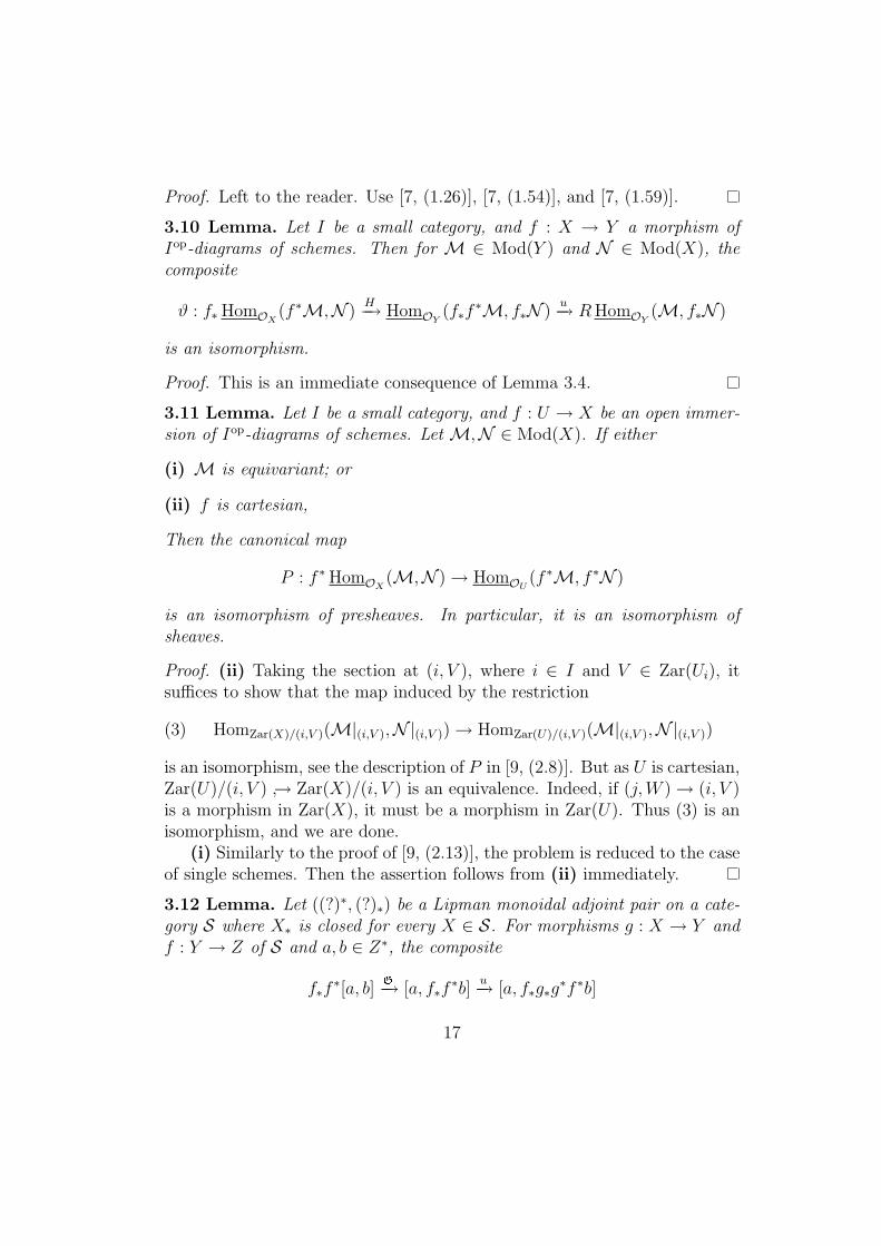
3.10 Lemma. Let I be a small category, and f : X → Y a morphism ofIop-diagrams of schemes. Then for M ∈ Mod(Y ) and N ∈ Mod(X), thecomposite

ϑ : f∗HomOX (f ∗M,N )H−→ HomOY (f∗f ∗M, f∗N )

u−→ RHomOY (M, f∗N )

is an isomorphism.

Proof. This is an immediate consequence of Lemma 3.4.

3.11 Lemma. Let I be a small category, and f : U → X be an open immer-sion of Iop-diagrams of schemes. Let M,N ∈ Mod(X). If either

(i) M is equivariant; or

(ii) f is cartesian,

Then the canonical map

P : f ∗HomOX (M,N )→ HomOU (f ∗M, f ∗N )

is an isomorphism of presheaves. In particular, it is an isomorphism ofsheaves.

Proof. (ii) Taking the section at (i, V ), where i ∈ I and V ∈ Zar(Ui), itsuffices to show that the map induced by the restriction

(3) HomZar(X)/(i,V )(M|(i,V ),N|(i,V ))→ HomZar(U)/(i,V )(M|(i,V ),N|(i,V ))

is an isomorphism, see the description of P in [9, (2.8)]. But as U is cartesian,Zar(U)/(i, V ) ↪→ Zar(X)/(i, V ) is an equivalence. Indeed, if (j,W )→ (i, V )is a morphism in Zar(X), it must be a morphism in Zar(U). Thus (3) is anisomorphism, and we are done.

(i) Similarly to the proof of [9, (2.13)], the problem is reduced to the caseof single schemes. Then the assertion follows from (ii) immediately.

3.12 Lemma. Let ((?)∗, (?)∗) be a Lipman monoidal adjoint pair on a cate-gory S where X∗ is closed for every X ∈ S. For morphisms g : X → Y andf : Y → Z of S and a, b ∈ Z∗, the composite

f∗f ∗[a, b]G−→ [a, f∗f ∗b]

u−→ [a, f∗g∗g∗f ∗b]

17

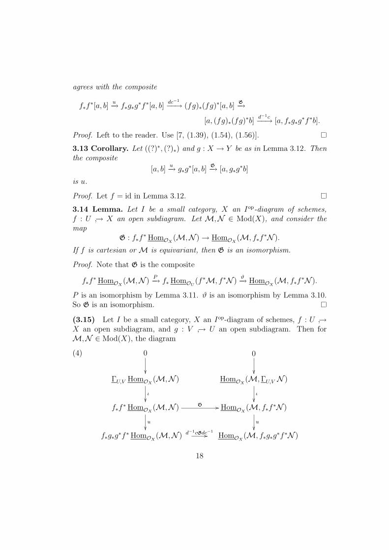
agrees with the composite

f∗f ∗[a, b]u−→ f∗g∗g∗f ∗[a, b]

dc−1−−→ (fg)∗(fg)∗[a, b]G−→

[a, (fg)∗(fg)∗b]d−1c−−→ [a, f∗g∗g∗f ∗b].

Proof. Left to the reader. Use [7, (1.39), (1.54), (1.56)].

3.13 Corollary. Let ((?)∗, (?)∗) and g : X → Y be as in Lemma 3.12. Thenthe composite

[a, b]u−→ g∗g∗[a, b]

G−→ [a, g∗g∗b]

is u.

Proof. Let f = id in Lemma 3.12.

3.14 Lemma. Let I be a small category, X an Iop-diagram of schemes,f : U ↪→ X an open subdiagram. Let M,N ∈ Mod(X), and consider themap

G : f∗f ∗HomOX (M,N )→ HomOX (M, f∗f ∗N ).

If f is cartesian or M is equivariant, then G is an isomorphism.

Proof. Note that G is the composite

f∗f ∗HomOX (M,N )P−→ f∗HomOU (f ∗M, f ∗N )

ϑ−→ HomOX (M, f∗f ∗N ).

P is an isomorphism by Lemma 3.11. ϑ is an isomorphism by Lemma 3.10.So G is an isomorphism.

(3.15) Let I be a small category, X an Iop-diagram of schemes, f : U ↪→X an open subdiagram, and g : V ↪→ U an open subdiagram. Then forM,N ∈ Mod(X), the diagram

(4) 0

��

0

��ΓU,V HomOX (M,N )

ι

��

HomOX (M,ΓU,V N )

ι

��f∗f ∗HomOX (M,N )

u

��

G // HomOX (M, f∗f ∗N )

u

��f∗g∗g∗f ∗HomOX (M,N ) d−1cGdc−1

// HomOX (M, f∗g∗g∗f ∗N )

18

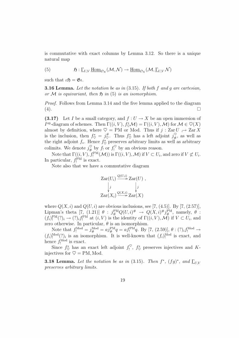
is commutative with exact columns by Lemma 3.12. So there is a uniquenatural map

(5) H : ΓU,V HomOX (M,N )→ HomOX (M,ΓU,V N )

such that ιH = Gι.

3.16 Lemma. Let the notation be as in (3.15). If both f and g are cartesian,or M is equivariant, then H in (5) is an isomorphism.

Proof. Follows from Lemma 3.14 and the five lemma applied to the diagram(4).

(3.17) Let I be a small category, and f : U → X be an open immersion ofIop-diagram of schemes. Then Γ((i, V ), f ∗♥M) = Γ((i, V ),M) forM∈ ♥(X)almost by definition, where ♥ = PM or Mod. Thus if j : ZarU ↪→ ZarXis the inclusion, then f ∗♥ = j#

♥ . Thus f ∗♥ has a left adjoint j♥#, as well asthe right adjoint f∗. Hence f ∗♥ preserves arbitrary limits as well as arbitrary

colimits. We denote j♥# by f! or f♥! by an obvious reason.

Note that Γ((i, V ), fPM! (M)) is Γ((i, V ),M) if V ⊂ Ui, and zero if V 6⊂ Ui.

In particular, fPM! is exact.

Note also that we have a commutative diagram

Zar(Ui)Q(U,i) //

j

��

Zar(U)

j

��Zar(Xi)

Q(X,i)// Zar(X)

,

where Q(X, i) and Q(U, i) are obvious inclusions, see [7, (4.5)]. By [7, (2.57)],Lipman’s theta [7, (1.21)] θ : jPM

# Q(U, i)# → Q(X, i)#jPM# , namely, θ :

(fi)PM! (?)i → (?)if

PM! at (i, V ) is the identity of Γ((i, V ),M) if V ⊂ Ui, and

zero otherwise. In particular, θ is an isomorphism.Note that fMod

! = jMod# = ajPM

# q = afPM! q. By [7, (2.59)], θ : (?)if

Mod! →

(fi)Mod! (?)i is an isomorphism. It is well-known that (fi)

Mod! is exact, and

hence fMod! is exact.

Since f ∗♥ has an exact left adjoint f♥! , f ∗♥ preserves injectives and K-injectives for ♥ = PM,Mod.

3.18 Lemma. Let the notation be as in (3.15). Then f ∗, (fg)∗, and ΓU,Vpreserves arbitrary limits.

19

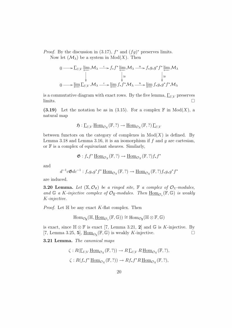
Proof. By the discussion in (3.17), f ∗ and (fg)∗ preserves limits.Now let (Mλ) be a system in Mod(X). Then

0 // ΓU,V lim←−Mλ

��

ι // f∗f ∗ lim←−Mλ

∼=��

u // f∗g∗g∗f ∗ lim←−Mλ

∼=��

0 // lim←−ΓU,V Mλι // lim←− f∗f

∗Mλu // lim←− f∗g∗g

∗f ∗Mλ

is a commutative diagram with exact rows. By the five lemma, ΓU,V preserveslimits.

(3.19) Let the notation be as in (3.15). For a complex F in Mod(X), anatural map

H : ΓU,V HomOX (F, ?)→ HomOX (F, ?) ΓU,V

between functors on the category of complexes in Mod(X) is defined. ByLemma 3.18 and Lemma 3.16, it is an isomorphism if f and g are cartesian,or F is a complex of equivariant sheaves. Similarly,

G : f∗f ∗HomOX (F, ?)→ HomOX (F, ?)f∗f ∗

andd−1cGdc−1 : f∗g∗g∗f ∗HomOX (F, ?)→ HomOX (F, ?)f∗g∗g∗f ∗

are induced.

3.20 Lemma. Let (X,OX) be a ringed site, F a complex of OX-modules,and G a K-injective complex of OX-modules. Then HomOX(F,G) is weaklyK-injective.

Proof. Let H be any exact K-flat complex. Then

HomOX(H,HomOX(F,G)) ∼= HomOX(H⊗ F,G)

is exact, since H ⊗ F is exact [7, Lemma 3.21, 2] and G is K-injective. By[7, Lemma 3.25, 5], HomOX(F,G) is weakly K-injective.

3.21 Lemma. The canonical maps

ζ : R(ΓU,V HomOX (F, ?))→ RΓU,V RHomOX (F, ?),

ζ : R(f∗f ∗HomOX (F, ?))→ Rf∗f ∗RHomOX (F, ?),

20

andζ : R(f∗g∗g∗f ∗HomOX (F, ?))→ Rf∗Rg∗g∗f ∗RHomOX (F, ?)

are isomorphisms.

Proof. For a K-injective complex G, HomOX (F,G) is weakly K-injective. Soit is K-flabby, and ΓU,V -acyclic [9, (4.3)]. In particular, f ∗HomOX (F,G) andg∗f ∗HomOX (F,G) are K-limp by [9, (4.6)], and the assertion follows.

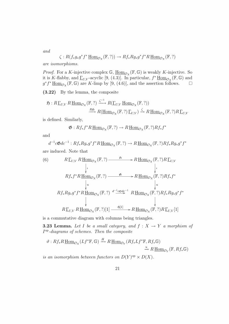
(3.22) By the lemma, the composite

H : RΓU,V RHomOX (F, ?)ζ−1−−→ R(ΓU,V HomOX (F, ?))

RH−−→ R(HomOX (F, ?) ΓU,V )ζ−→ RHomOX (F, ?)RΓU,V

is defined. Similarly,

G : Rf∗f ∗RHomOX (F, ?)→ RHomOX (F, ?)Rf∗f ∗

and

d−1cGdc−1 : Rf∗Rg∗g∗f ∗RHomOX (F, ?)→ RHomOX (F, ?)Rf∗Rg∗g∗f ∗

are induced. Note that

(6) RΓU,V RHomOX (F, ?) H //

ι

��

RHomOX (F, ?)RΓU,V

ι

��Rf∗f ∗RHomOX (F, ?) G //

u

��

RHomOX (F, ?)Rf∗f ∗

u

��Rf∗Rg∗g∗f ∗RHomOX (F, ?) d−1cGdc−1

//

��

RHomOX (F, ?)Rf∗Rg∗g∗f ∗

��RΓU,V RHomOX (F, ?)[1]

H[1] // RHomOX (F, ?)RΓU,V [1]

is a commutative diagram with columns being triangles.

3.23 Lemma. Let I be a small category, and f : X → Y a morphism ofIop-diagrams of schemes. Then the composite

ϑ : Rf∗RHomOX (Lf ∗F,G)H−→ RHomOY (Rf∗Lf ∗F, Rf∗G)

u−→ RHomOY (F, Rf∗G)

is an isomorphism between functors on D(Y )op ×D(X).

21

Proof. This is an immediate consequence of [7, (1.49)] and [7, (8.23), 5].

3.24 Corollary. Let f : U → X be a cartesian open immersion. Then

P : f ∗RHomOX (F,G)→ RHomOU (f ∗F, f ∗G)

is an isomorphism for any F,G ∈ D(X).

Proof. If G is a K-injective complex in K(X), then so is f ∗G by (3.17). Soit suffices to show that

f ∗HomOX (F,G)→ HomOU (f ∗F, f ∗G)

is an isomorphism of complexes, if F and G are complexes in Mod(X). Thisfollows from Lemma 3.11 and the fact that f ∗ preserves direct product.

3.25 Lemma. Let I be a small category, and f : X → Y a morphism ofIop-diagrams of schemes. Let F and G be objects in D(Y ). Assume that oneof the following holds:

(i) f is locally an open immersion, F ∈ DEM(Y ), and one of the followingholds:

(a) G ∈ D+(Y );

(b) F ∈ D+EM(Y );

(c) G ∈ DLqc(Y ).

(ii) f is flat, Y is locally noetherian, G ∈ D+(Y ), and F ∈ D−Coh(Y ).

(iii) f is flat, Y is locally noetherian, F ∈ DCoh(Y ), and both G and f ∗Ghave finite injective dimension.

Then the canonical map

P : f ∗RHomOY (F,G)→ RHomOX (f ∗F, f ∗G)

is an isomorphism.

22

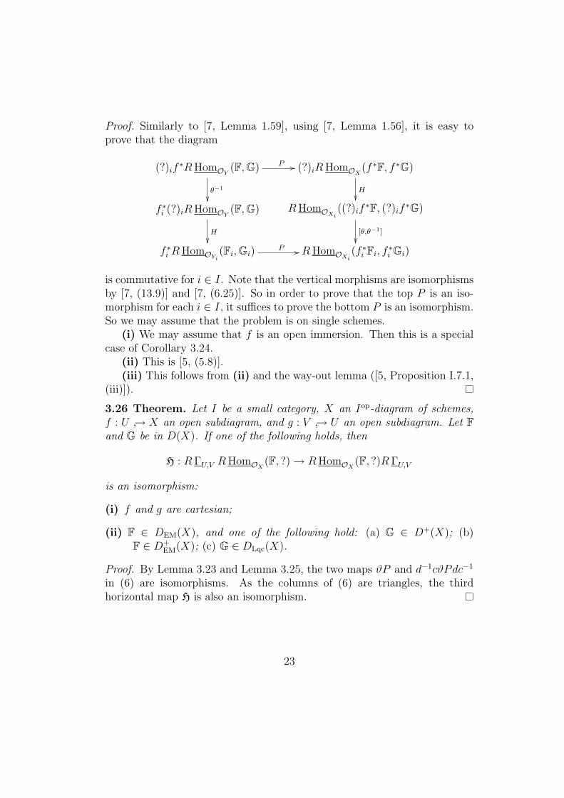
Proof. Similarly to [7, Lemma 1.59], using [7, Lemma 1.56], it is easy toprove that the diagram

(?)if∗RHomOY (F,G) P //

θ−1

��

(?)iRHomOX (f ∗F, f ∗G)

H��

f ∗i (?)iRHomOY (F,G)

H��

RHomOXi ((?)if∗F, (?)if

∗G)

[θ,θ−1]��

f ∗i RHomOYi (Fi,Gi)P // RHomOXi (f

∗i Fi, f ∗i Gi)

is commutative for i ∈ I. Note that the vertical morphisms are isomorphismsby [7, (13.9)] and [7, (6.25)]. So in order to prove that the top P is an iso-morphism for each i ∈ I, it suffices to prove the bottom P is an isomorphism.So we may assume that the problem is on single schemes.

(i) We may assume that f is an open immersion. Then this is a specialcase of Corollary 3.24.

(ii) This is [5, (5.8)].(iii) This follows from (ii) and the way-out lemma ([5, Proposition I.7.1,

(iii)]).

3.26 Theorem. Let I be a small category, X an Iop-diagram of schemes,f : U ↪→ X an open subdiagram, and g : V ↪→ U an open subdiagram. Let Fand G be in D(X). If one of the following holds, then

H : RΓU,V RHomOX (F, ?)→ RHomOX (F, ?)RΓU,V

is an isomorphism:

(i) f and g are cartesian;

(ii) F ∈ DEM(X), and one of the following hold: (a) G ∈ D+(X); (b)F ∈ D+

EM(X); (c) G ∈ DLqc(X).

Proof. By Lemma 3.23 and Lemma 3.25, the two maps ϑP and d−1cϑPdc−1

in (6) are isomorphisms. As the columns of (6) are triangles, the thirdhorizontal map H is also an isomorphism.

23

4. Matlis duality and the local duality

Let S be a scheme, G an S-group scheme, (X,Y ) a standard G-local G-scheme. That is, X is a standard G-local G-scheme, and Y is its uniqueminimal closed G-subscheme. We denote the inclusion Y ↪→ X by j.

We denote the defining ideal sheaf of Y by I. Thus I is the unique G-maximal G-ideal of OX . We fix the generic point of an irreducible componentof Y and denote it by η.

4.1 Lemma. Let C be a class of noetherian local rings. Assume that if A ∈ Cand B is essentially of finite type over A, then B ∈ C. Let P(A,M) be aproperty of a pair (A,M) of a finitely generated module M over a noetherianlocal ring A such that A ∈ C. Assume that

(i) If A ∈ C, P(A,M) holds, and P ∈ SpecA, then P(AP ,MP ) holds.

(ii) If A ∈ C, M a finite A-module, and A → B is a flat local homomor-phism essentially of finite type with local complete intersection fibers(resp. geometrically regular fibers), then P(A,M) holds if and only ifP(B,B ⊗AM) holds.

Assume that the all local rings of X belong to C. For M ∈ Coh(G,X), ifP(OX,η,Mη) holds (resp. P(OX,η,Mη) holds and either the second projectionp2 : G ×X → X is smooth or S = Spec k with k a perfect field and G is offinite type over S), then P(OX,x,Mx) holds for any x ∈ X.

Proof. Let Z be the unique integral closed subscheme of X whose genericpoint is x. Let Z∗ be the unique minimal closed G-subscheme of X containingZ, see [8]. As η ∈ Y ⊂ Z∗, there exists some irreducible component Z0 of Zsuch that η ∈ Z0. Let ζ be the generic point of Z0. Since P(OX,η,Mη) holdsand ζ is a generalization of η, P(OX,ζ ,Mζ) holds. Then by [8, Corollary 7.6],P(OX,x,Mx) holds.

4.2 Corollary. Let m, n, and g be non-negative integers or ∞. Then

(i) Let M∈ Coh(G,X), and assume that Mη is maximal Cohen–Macaulay(resp. of finite injective dimension, projective dimension m, dim− depth =n, torsionless, reflexive, G-dimension g, zero) as an OX,η-module. ThenMx is so as an OX,x-module for any x ∈ X.

(ii) If OX,η is a complete intersection, then X is locally a complete intersec-tion.

24

(iii) Assume that p2 : G×X → X is smooth or S = Spec k with k a perfectfield and G is of finite type over S. If OX,η is regular, then X is regular.

(iv) In addition to the assumption of (iii), assume further that X is a locallyexcellent Fp-scheme, where p is a prime number. If OX,η is F -regular(resp. F -rational), then the all local rings of X is F -regular (resp. F -rational).

Proof. (i) Let C be the class of all noetherian local rings, and P(A,M) be“M is a maximal Cohen–Macaulay A-module.” We can apply Lemma 4.1.Similarly for other properties.

(ii) Let C be the class of all noetherian local rings, and P(A,M) be “A isa complete intersection.” Then as P(OX,η, 0) holds, P(OX,x, 0) holds for anyx ∈ X.

(iii) Let C be the class of all noetherian local rings, and P(A,M) be “Ais regular.”

(iv) Let C be the class of all excellent noetherian local rings of charac-teristic p, and P(A,M) be “A is F -regular” (resp. “A is F -rational”).

4.3 Corollary. The stalk functor (?)η : Qch(G,X) → Mod(OX,η) is faith-fully exact.

Proof. The exactness is well-known. Let M ∈ Qch(G,X) and assume thatM 6= 0. Then as Qch(G,X) is locally noetherian and its noetherian objectis nothing but a coherent (G,OX)-module, M contains a nonzero coherent(G,OX)-submodule N . Then by Corollary 4.2, Mη ⊃ Nη 6= 0. This showsthat (?)η is faithfully exact.

4.4 Remark. Formally, (?)η is a functor from Qch(G,X) = Qch(BMG (X)), or

more generally, from Mod(G,X) = Mod(BMG (X)) to Mod(OX,η), and is the

composite

Mod(BMG (X))

(?)0−−→ Mod(BMG (X)0) = Mod(X0)

h∗−→ Mod(SpecOX,η),where h : SpecOX,η → X0 is the inclusion. Thus (?)η is sometimes writtenas (?)η(?)0, where (?)η means h∗.

4.5 Corollary (G-NAK). Let M∈ Coh(G,X). If j∗M = 0, then M = 0,where j : Y ↪→ X is the inclusion.

Proof. Since j∗M = 0, M/IM = 0. So Mη/IηMη = 0. By Nakayama’slemma, Mη = 0. By Corollary 4.3, M = 0.

25

4.6 Proposition. A standard G-artinian G-scheme is Cohen–Macaulay.

Proof. By Lemma 2.20, we may assume that the G-scheme is G-local. So letX be a G-artinian G-local standard G-scheme. Let Y , η, and I be as above.

Then G√

0 = I, since I is the only G-prime ideal (for the definition andbasic properties of G

√?, see [8, section 4]). So Y = X, set theoretically.

Thus η is the generic point of an irreducible component of X. So OX,ηis an artinian ring, and hence is Cohen–Macaulay. By Corollary 4.2, X isCohen–Macaulay.

4.7 Corollary. Y is Cohen–Macaulay.

Proof. Since Y is G-artinian G-local standard, the corollary follows immedi-ately from Proposition 4.6.

(4.8) From now on, we assume that X has a G-dualizing complex IX (see[7, (31.15)]). For a G-morphism f : X ′ → X which is separated of finite type,we denote f !IX by IX′ , where f ! is the twisted inverse functor BG

M(f)! (see [7,chapter 29]). Note that IX′ is a G-dualizing complex of X ′ [7, Lemma 31.11].By [7, Lemma 31.6], IX′ , viewed as a complex of OX′-modules, is a dualizingcomplex of X ′.

Since OY,η is Cohen–Macaulay, there is only one i such that H i(IY )η 6= 0.This is equivalent to say that H i(IY ) 6= 0. If this i is 0, then we say that IXis G-normalized. If X has a G-dualizing complex, then by shifting, X has aG-normalized G-dualizing complex.

From now on, we always assume that IX is G-normalized.

4.9 Lemma. IX,η is a normalized dualizing complex of the local ring OX,η.In particular, H0

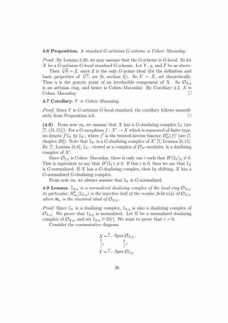
mη(IX,η) is the injective hull of the residue field κ(η) of OX,η,where mη is the maximal ideal of OX,η.Proof. Since IX is a dualizing complex, IX,η is also a dualizing complex ofOX,η. We prove that IX,η is normalized. Let D be a normalized dualizingcomplex of OX,η, and set IX,η ∼= D[r]. We want to prove that r = 0.

Consider the commutative diagram

X SpecOX,ηpoo

Y

j

OO

SpecOY,ηj′

OO

qoo

.

26

By the commutativity with restrictions [7, Proposition 18.14],

H0(IY )η ∼= H0(q∗j!IX) ∼= H0((j′)!IX,η) ∼= ExtrOX,η(OY,η,D) 6= 0.

The Matlis dual of the last module is H−rmη (OY,η), by the local duality [5,(V.6.3)]. SinceOY,η is anOX,η-module of finite length, H−rmη (OY,η) 6= 0 impliesr = 0.

4.10 Lemma. H iY (IX) = 0 for i 6= 0, and H0

Y (IX)η is the injective hull ofthe residue field κ(η) of the local ring OX,η.Proof. By [9, Theorem 6.10],

(H iY (IX))η ∼= H i((?)ηRΓY IX) ∼= H i(RΓIη(?)ηIX) ∼= H i

mη(IX,η).

Since IX,η is a normalized dualizing complex of OX,η, the last module is zeroif i 6= 0 and is the injective hull of the residue field κ(η) of the local ring OX,ηif i = 0. As (?)η is faithfully exact, we are done.

(4.11) We set E := H0Y (IX), and call it the G-sheaf of Matlis. Note that

the definition of E depends on the choice of IX . Note also that Eη is theinjective hull of the residue field of OX,η.4.12 Lemma. E is of finite injective dimension as an object of Mod(G,X).

Proof. We may assume that IX is a bounded complex of injective objects. ByLemma 4.10, E is isomorphic to ΓY (IX) in D(X). On the other hand, ΓY (IX)is quasi-isomorphic to J = Cone(IX → f∗f ∗IX)[−1], where f : X \ Y → Xis the inclusion. As f∗f ∗ has an exact left adjoint f!f

∗ (see (3.17)), J is abounded injective resolution of E .

4.13 Lemma. ExtiOX (M, E) = 0 for i > 0 and M∈ Coh(G,X).

Proof. ExtiOX (M, E)η ∼= ExtiOX,η(Mη, Eη). As Eη is injective, we are done.

4.14 Corollary. D := HomOX (?, E) is an exact functor on Coh(G,X).

4.15 Lemma. For M∈ Qch(G,X), the following are equivalent:

(i) M is of finite length;

(ii) M∈ Coh(G,X), and InM = 0 for some n.

27

(iii) Mη is an OX,η-module of finite length;

Proof. (i)⇒(ii) As M is of finite length, it is a noetherian object. Hence itis coherent by [7, Lemma 12.8]. As M is also an artinian object, InM =In+1M for sufficiently large n. By Corollary 4.5, InM = 0.

(ii)⇒(iii) As M is coherent, Mη is a finitely generated OX,η-module.Since InηMη = 0, the support ofMη is one point, and henceMη is a moduleof finite length.

(iii)⇒(i) This is because (?)η is faithfully exact.

(4.16) We denote by F the full subcategory of those objectsM∈ Qch(G,X)such that the equivalent conditions in the lemma are satisfied.

4.17 Theorem (Matlis duality). Set D := HomOX (?, E). Then

(i) D is an exact functor from F to itself.

(ii) D2 ∼= Id as functors on F . In particular, D : F → F is an anti-equivalence.

Proof. (i) If M ∈ F , then D(M) = HomOX (M, E) is in Qch(G,X), andHomOX (M, E)η = HomOX,η(Mη, Eη) is of finite length, because this module isthe Matlis dual of the moduleMη, which is of finite length. So the condition(iii) in Lemma 4.15 is satisfied, and hence D(M) ∈ F . The exactness of Dis already checked.

(ii) Let D : M→ DDM = HomOX (HomOX (M, E), E) be the canonicalmap, see (2.2). Note that by Lemma 2.5 and Lemma 2.7, applying (?)η tothis map, we get the duality map D :Mη → HomOX,η(HomOX,η(Mη, Eη), Eη),which is an isomorphism, since Eη is the injective hull of the residue field κ(η).Since (?)η is faithful, D :M→ DDM is an isomorphism.

4.18 Theorem (Local duality). For F ∈ DCoh(G,X), the composite

d : RΓY FD−→ RΓY RHomOX (RHomOX (F, IX), IX)

H−→RHomOX (RHomOX (F, IX), RΓY IX) ∼= RHomOX (RHomOX (F, IX), E)

is an isomorphism. It induces an isomorphism

H iY (F) ∼= HomOX (Ext−iOX (F, IX), E)

for each i ∈ Z.

28

Proof. D in the composition is an isomorphism by [7, (31.9)]. H is an iso-morphism by Theorem 3.26, (i). Thus d is an isomorphism.

To prove the second assertion, it suffices to show that

ExtiOX (G, E) ∼= HomOX (H−i(G), E),

where G = RHomOX (F, IX). Note that G ∈ DCoh(X) by [7, (31.9)]. Let J bea bounded injective resolution of E (it does exist, see Lemma 4.12). Considerthe spectral sequence

Ep,q2 = Hp(HomOX (H−q(G), J))⇒ Extp+qOX (G, E).

By Lemma 4.13, Ep,q2 = 0 for p 6= 0, and the spectral sequence collapses, and

we get the desired assertion.

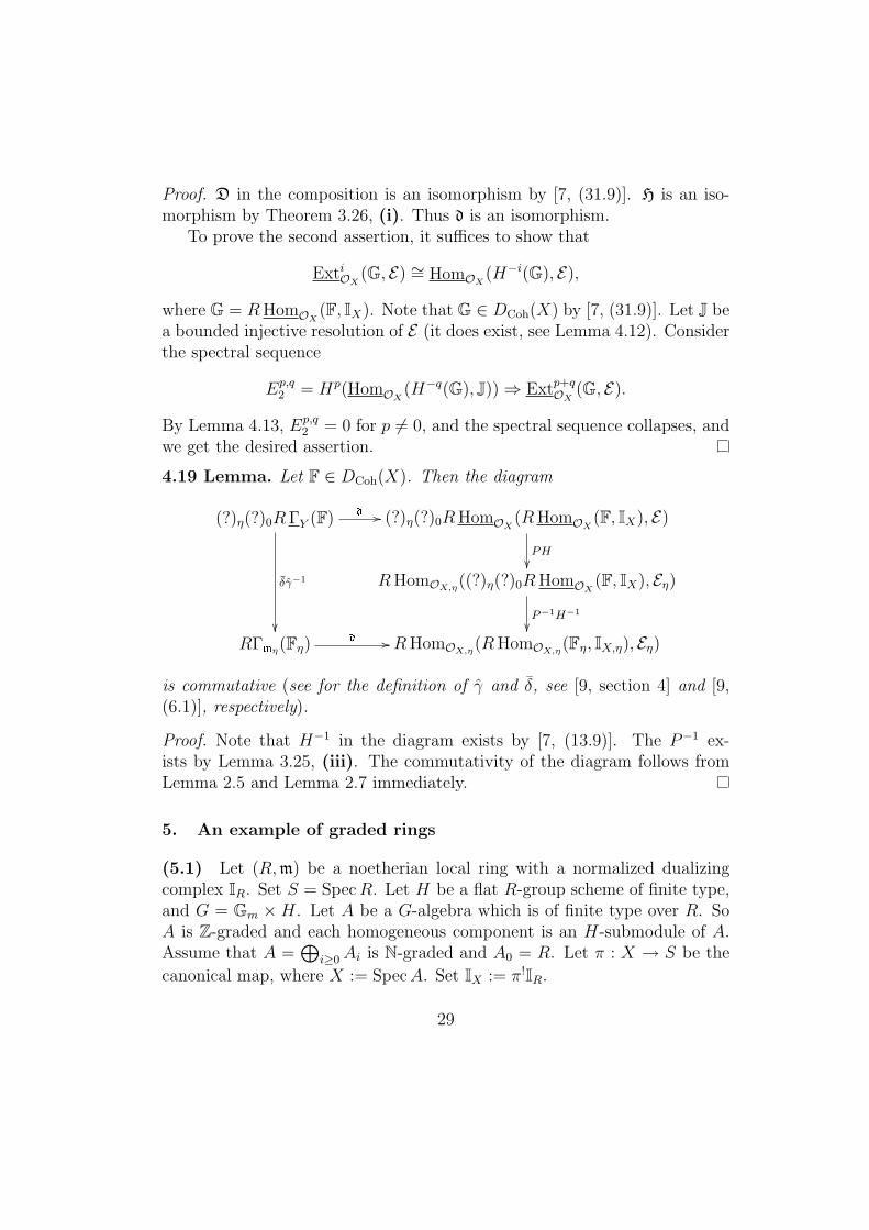
4.19 Lemma. Let F ∈ DCoh(X). Then the diagram

(?)η(?)0RΓY (F) d //

δ̄γ̂−1

��

(?)η(?)0RHomOX (RHomOX (F, IX), E)

PH��

RHomOX,η((?)η(?)0RHomOX (F, IX), Eη)P−1H−1

��RΓmη(Fη)

d // RHomOX,η(RHomOX,η(Fη, IX,η), Eη)

is commutative (see for the definition of γ̂ and δ̄, see [9, section 4] and [9,(6.1)], respectively).

Proof. Note that H−1 in the diagram exists by [7, (13.9)]. The P−1 ex-ists by Lemma 3.25, (iii). The commutativity of the diagram follows fromLemma 2.5 and Lemma 2.7 immediately.

5. An example of graded rings

(5.1) Let (R,m) be a noetherian local ring with a normalized dualizingcomplex IR. Set S = SpecR. Let H be a flat R-group scheme of finite type,and G = Gm ×H. Let A be a G-algebra which is of finite type over R. SoA is Z-graded and each homogeneous component is an H-submodule of A.Assume that A =

⊕i≥0 Ai is N-graded and A0 = R. Let π : X → S be the

canonical map, where X := SpecA. Set IX := π!IR.

29

5.2 Lemma. Under the notation as above, X is G-local, and IX is G-normalized.

Proof. Let I be a proper G-ideal of A. Then I is a homogeneous ideal,and is contained in the unique graded maximal ideal M := m + A+, whereA+ =

⊕i>0 Ai. Clearly, M is a G-ideal, and hence is the unique G-maximal

G-ideal. So X is G-local.Let ϕ : S → X be the closed immersion induced by A→ A/A+ = R. Let

ψ : Y → S be the closed immersion induced by R → R/m ∼= A/M, whereY = SpecA/M. Then since πϕ = idS,

IY = (ϕψ)!(IX) = ψ!ϕ!π!IR = ψ!IR.

So H i(IY ) ∼= ExtiR(R/m, IR), whose Matlis dual is H im(R/m). This is nonzero

if and only if i = 0. Thus IX is G-normalized.

(5.3) For a finite R-module V , set V † := HomR(V,ER), where ER is theinjective hull of the residue field R/m of R. For an A-finite G-module M ,set M∨ = lim−→HomR(M/MnM,ER). As each M/MnM is an R-finite (G,A)-module, each HomR(M/MnM,ER) is a (G,A)-module, and hence M∨ is alsoa (G,A)-module. It is easy to see that M∨ ∼= HomA(M,A∨). Note that thedegree i component of M∨ is M †

−i. That is, M∨ =⊕

i∈ZM†−i.

5.4 Lemma. A∨ is isomorphic to EA := Γ(X, E) as a (G,A)-module.

Proof. We may assume that IR is the normalized fundamental dualizing com-plex. We have

(7) E = H0Y (IX) = lim−→Ext0

OX (OX/In, IX)

= lim−→H0((ψn)∗ψ!nπ

!IS) = lim−→Ext0R(A/Mn, IR) ,̃

where ψn : SpecA/Mn → SpecA is the canonical closed immersion, and (?)˜denotes the quasi-coherent sheaf associated to a module. On the other hand,A/Mn has finite length as an R-module, so

Ext0R(A/Mn, IR) ∼= H0(HomR(A/Mn, IR)) ∼= H0(HomR(A/Mn,ΓmIR))

∼= H0(HomR(A/Mn, ER)) = HomR(A/Mn, ER).

We prove that the map HomR(A/Mm, ER) → HomR(A/Mn, ER) in theinductive system is induced by the projection A/Mn → A/Mm for n ≥ m.

30

Note that Ext0OX (OX/Im, IX)→ Ext0

OX (OX/In, IX) in (7) is induced by theprojection. So by the description of the twisted inverse for finite morphisms[7, (27.7)], the map (ψm)∗ψ!

m → (ψn)∗ψ!n is induced by the counit map. That

is, the map is the composite

(ψm)∗ψ!m∼= (ψn)∗(ψn,m)∗ψ!

n,mψ!n

ε−→ (ψn)∗ψ!n,

where ψn,m : SpecA/Mm → SpecA/Mn is the map induced by the projec-tion. So again by [7, (27.7)], the map Ext0

R(A/Mm, IR) → Ext0R(A/Mn, IR)

in (7) is also induced by the projection, and we are done.Hence

EA = lim−→HomR(A/Mn, ER) = A∨.

5.5 Corollary. Assume that A is Cohen–Macaulay and dimA = d. SetΓ(X,H−d(IX)) to be ωA. For a A-finite (G,A)-module M , the canonicalmap

d : H iM(M)→ Extd−iA (M,ωA)∨

is an isomorphism of (G,A)-modules. That is, this isomorphism preservesgrading and H-action.

5.6 Remark. Assume that R = k is a field. Let G be the full subcategory of(G,A)-modules consisting of M such that Mi is finite dimensional for everyi. Then we define M∨ =

⊕i∈ZM

†−i for M ∈ G, where M †

−i = Homk(M−i, k).We have an isomorphism Φ : ∗HomA(M,A∨) → M∨. See for the notation∗HomA, [1]. Note that

Φn : ∗HomA(M,A∨)n = ∗HomA(M(−n), A∨)0

→ Homk(M−n, A∨0 ) = Homk(M−n, k)

is given by the restriction. It is easy to see that (?)∨ is an anti-equivalencefrom G to itself. This also gives an anti-equivalence between the category ofnoetherian (G,A)-modules to that of artinian (G,A)-modules. This is notcontained in Theorem 4.17, which treats only objects of finite length.

5.7 Example. Let k be an algebraically closed field of characteristic two,and we set R = k and S = SpecR. Let V = k2, and H = GL(V ). LetA = SymV , and X = V ∗ = SpecA. Then A∗2 is not injective as a G-module.So EA =

⊕i≥0 A

∗i is not injective as a G-module either. So EA is not injective

as a (G,A)-module either by [6, Corollary II.1.1.9]. In particular, EA is notthe injective hull of A/M as a (G,A)-module.

31

References

[1] W. Bruns and J. Herzog, Cohen–Macaulay Rings (first paperback edi-tion), Cambridge (1998).

[2] J. Franke, On the Brown representability theorem for triangulated cat-egories, Topology 40 (2001), 667–680.

[3] S. Goto and K.-i. Watanabe, On graded rings, I, J. Math. Soc. Japan30 (1978), 179–213.

[4] S. Goto and K.-i. Watanabe, On graded rings, II (Zn-graded rings),Tokyo J. Math. 1 (1978), 237–261.

[5] R. Hartshorne, Residues and Duality, Lecture Notes in Math. 20,Springer, (1966).

[6] M. Hashimoto, Auslander-Buchweitz Approximations of EquivariantModules, London Mathematical Society Lecture Note Series 282, Cam-bridge (2000).

[7] M. Hashimoto, Equivariant Twisted Inverses, Foundations ofGrothendieck Duality for Diagrams of Schemes (J. Lipman, M.Hashimoto), Lecture Notes in Math. 1960, Springer (2009), pp. 261–478.

[8] M. Hashimoto and M. Miyazaki, G-prime and G-primary G-ideals onG-schemes, preprint arXiv:0906.1441v2

[9] M. Hashimoto and M. Ohtani, Local cohomology on diagrams ofschemes, Michigan Math. J. 57 (2008), 383–425.

[10] Y. Kamoi, Noetherian rings graded by an abelian group, Tokyo J. Math.18 (1995), 31–48.

[11] J. Lipman, Notes on Derived Functors and Grothendieck Duality, Foun-dations of Grothendieck Duality for Diagrams of Schemes (J. Lipman,M. Hashimoto), Lecture Notes in Math. 1960, Springer (2009), pp. 1–259.

32