Embed Size (px)
Citation preview

Aswath Damodaran 1
Equity Instruments & Markets: Part IDiscounted Cash Flow Valuation
B40.3331Aswath Damodaran

Aswath Damodaran 2
Discounted Cashflow Valuation: Basis forApproach
n where CFt is the cash flow in period t, and r is the discount rateappropriate given the riskiness of the cash flow and t is the life of theasset.
Proposition 1: For an asset to have value, the expected cash flowshave to be positive some time over the life of the asset.
Proposition 2: Assets that generate cash flows early in their life willbe worth more than assets that generate cash flows later; the lattermay however have greater growth and higher cash flows tocompensate.
Value = CF
t
( 1 +r)tt = 1
t = n∑

Aswath Damodaran 3
Equity Valuation versus Firm Valuation
n Value just the equity stake in the business
n Value the entire business, which includes, besides equity, the otherclaimholders in the firm

Aswath Damodaran 4
I.Equity Valuation
n The value of equity is obtained by discounting expected cashflows toequity, i.e., the residual cashflows after meeting all expenses, taxobligations and interest and principal payments, at the cost of equity,i.e., the rate of return required by equity investors in the firm.
where,
CF to Equityt = Expected Cashflow to Equity in period t
ke = Cost of Equity
n The dividend discount model is a specialized case of equity valuation,and the value of a stock is the present value of expected futuredividends.
Value of Equity = CF to Equityt
(1+ ke )tt=1
t=n
∑

Aswath Damodaran 5
II. Firm Valuation
n The value of the firm is obtained by discounting expected cashflows tothe firm, i.e., the residual cashflows after meeting all operatingexpenses and taxes, but prior to debt payments, at the weightedaverage cost of capital, which is the cost of the different componentsof financing used by the firm, weighted by their market valueproportions.
where,
CF to Firmt = Expected Cashflow to Firm in period t
WACC = Weighted Average Cost of Capital
Value of Firm = CF to Firm t
( 1 +WACC) tt = 1
t = n
∑

Aswath Damodaran 6
Firm Value and Equity Value
n To get from firm value to equity value, which of the following wouldyou need to do?
o Subtract out the value of long term debt
o Subtract out the value of all debt
o Subtract the value of all non-equity claims in the firm, that areincluded in the cost of capital calculation
o Subtract out the value of all non-equity claims in the firm
n Doing so, will give you a value for the equity which is
o greater than the value you would have got in an equity valuation
o lesser than the value you would have got in an equity valuation
o equal to the value you would have got in an equity valuation

Aswath Damodaran 7
Cash Flows and Discount Rates
n Assume that you are analyzing a company with the followingcashflows for the next five years.
Year CF to Equity Int Exp (1-t) CF to Firm
1 $ 50 $ 40 $ 90
2 $ 60 $ 40 $ 100
3 $ 68 $ 40 $ 108
4 $ 76.2 $ 40 $ 116.2
5 $ 83.49 $ 40 $ 123.49
Terminal Value $ 1603.008 $ 2363.008
n Assume also that the cost of equity is 13.625% and the firm canborrow long term at 10%. (The tax rate for the firm is 50%.)
n The current market value of equity is $1,073 and the value of debtoutstanding is $800.

Aswath Damodaran 8
Equity versus Firm Valuation
Method 1: Discount CF to Equity at Cost of Equity to get value of equity
n Cost of Equity = 13.625%
n PV of Equity = 50/1.13625 + 60/1.136252 + 68/1.136253 +76.2/1.136254 + (83.49+1603)/1.136255 = $1073
Method 2: Discount CF to Firm at Cost of Capital to get value of firm
Cost of Debt = Pre-tax rate (1- tax rate) = 10% (1-.5) = 5%
WACC = 13.625% (1073/1873) + 5% (800/1873) = 9.94%
PV of Firm = 90/1.0994 + 100/1.09942 + 108/1.09943 + 116.2/1.09944 +(123.49+2363)/1.09945 = $1873
n PV of Equity = PV of Firm - Market Value of Debt
= $ 1873 - $ 800 = $1073

Aswath Damodaran 9
First Principle of Valuation
n Never mix and match cash flows and discount rates.
n The key error to avoid is mismatching cashflows and discount rates,since discounting cashflows to equity at the weighted average cost ofcapital will lead to an upwardly biased estimate of the value of equity,while discounting cashflows to the firm at the cost of equity will yielda downward biased estimate of the value of the firm.

Aswath Damodaran 10
The Effects of Mismatching Cash Flows andDiscount Rates
Error 1: Discount CF to Equity at Cost of Capital to get equity value
n PV of Equity = 50/1.0994 + 60/1.09942 + 68/1.09943 + 76.2/1.09944 +(83.49+1603)/1.09945 = $1248
n Value of equity is overstated by $175.
Error 2: Discount CF to Firm at Cost of Equity to get firm value
n PV of Firm = 90/1.13625 + 100/1.136252 + 108/1.136253 +116.2/1.136254 + (123.49+2363)/1.136255 = $1613
n PV of Equity = $1612.86 - $800 = $813
n Value of Equity is understated by $ 260.
Error 3: Discount CF to Firm at Cost of Equity, forget to subtract outdebt, and get too high a value for equity
n Value of Equity = $ 1613
n Value of Equity is overstated by $ 540

Aswath Damodaran 11
Discounted Cash Flow Valuation: The Steps
n Estimate the discount rate or rates to use in the valuation• Discount rate can be either a cost of equity (if doing equity valuation) or a
cost of capital (if valuing the firm)
• Discount rate can be in nominal terms or real terms, depending uponwhether the cash flows are nominal or real
• Discount rate can vary across time.
n Estimate the current earnings and cash flows on the asset, to eitherequity investors (CF to Equity) or to all claimholders (CF to Firm)
n Estimate the future earnings and cash flows on the asset beingvalued, generally by estimating an expected growth rate in earnings.
n Estimate when the firm will reach “stable growth” and whatcharacteristics (risk & cash flow) it will have when it does.
n Choose the right DCF model for this asset and value it.

Aswath Damodaran 12
Generic DCF Valuation Model
Cash flowsFirm: Pre-debt cash flowEquity: After debt cash flows
Expected GrowthFirm: Growth in Operating EarningsEquity: Growth in Net Income/EPS
CF1 CF2 CF3 CF4 CF5
Forever
Firm is in stable growth:Grows at constant rateforever
Terminal Value
CFn.........
Discount RateFirm:Cost of Capital
Equity: Cost of Equity
ValueFirm: Value of Firm
Equity: Value of Equity
DISCOUNTED CASHFLOW VALUATION
Length of Period of High Growth

Aswath Damodaran 13
DividendsNet Income * Payout Ratio= Dividends
Expected GrowthRetention Ratio *Return on Equity
Dividend 1 Dividend 2 Dividend 3 Dividend 4 Dividend 5
Forever
Firm is in stable growth:Grows at constant rateforever
Terminal Value= Dividendn+1/(ke-gn)
Dividend n.........
Cost of Equity
Discount at Cost of Equity
Value of Equity
Riskfree Rate:- No default risk- No reinvestment risk- In same currency andin same terms (real or nominal as cash flows
+Beta- Measures market risk X
Risk Premium- Premium for averagerisk investment
Type of Business
Operating Leverage
FinancialLeverage
Base EquityPremium
Country RiskPremium
EQUITY VALUATION WITH DIVIDENDS

Aswath Damodaran 14
Cashflow to EquityNet Income- (Cap Ex - Depr) (1- DR)- Change in WC (!-DR)= FCFE
Expected GrowthRetention Ratio *Return on Equity
FCFE1 FCFE2 FCFE3 FCFE4 FCFE5
Forever
Firm is in stable growth:Grows at constant rateforever
Terminal Value= FCFEn+1/(ke-gn)
FCFEn.........
Cost of Equity
Financing WeightsDebt Ratio = DR
Discount at Cost of Equity
Value of Equity
Riskfree Rate:- No default risk- No reinvestment risk- In same currency andin same terms (real or nominal as cash flows
+Beta- Measures market risk X
Risk Premium- Premium for averagerisk investment
Type of Business
Operating Leverage
FinancialLeverage
Base EquityPremium
Country RiskPremium
EQUITY VALUATION WITH FCFE

Aswath Damodaran 15
Cashflow to FirmEBIT (1-t)- (Cap Ex - Depr)- Change in WC= FCFF
Expected GrowthReinvestment Rate* Return on Capital
FCFF1 FCFF2 FCFF3 FCFF4 FCFF5
Forever
Firm is in stable growth:Grows at constant rateforever
Terminal Value= FCFFn+1/(r-gn)
FCFFn.........
Cost of Equity Cost of Debt(Riskfree Rate+ Default Spread) (1-t)
WeightsBased on Market Value
Discount at WACC= Cost of Equity (Equity/(Debt + Equity)) + Cost of Debt (Debt/(Debt+ Equity))
Value of Operating Assets+ Cash & Non-op Assets= Value of Firm- Value of Debt= Value of Equity
Riskfree Rate :- No default risk- No reinvestment risk- In same currency andin same terms (real or nominal as cash flows
+Beta- Measures market risk X
Risk Premium- Premium for averagerisk investment
Type of Business
Operating Leverage
FinancialLeverage
Base EquityPremium
Country RiskPremium
VALUING A FIRM

Aswath Damodaran 16
Discounted Cash Flow Valuation:The Inputs
Aswath Damodaran

Aswath Damodaran 17
I. Estimating Discount Rates
DCF Valuation

Aswath Damodaran 18
Estimating Inputs: Discount Rates
n Critical ingredient in discounted cashflow valuation. Errors inestimating the discount rate or mismatching cashflows and discountrates can lead to serious errors in valuation.
n At an intuitive level, the discount rate used should be consistent withboth the riskiness and the type of cashflow being discounted.• Equity versus Firm: If the cash flows being discounted are cash flows to
equity, the appropriate discount rate is a cost of equity. If the cash flowsare cash flows to the firm, the appropriate discount rate is the cost ofcapital.
• Currency: The currency in which the cash flows are estimated should alsobe the currency in which the discount rate is estimated.
• Nominal versus Real: If the cash flows being discounted are nominal cashflows (i.e., reflect expected inflation), the discount rate should be nominal

Aswath Damodaran 19
Cost of Equity
n The cost of equity should be higher for riskier investments and lowerfor safer investments
n While risk is usually defined in terms of the variance of actual returnsaround an expected return, risk and return models in finance assumethat the risk that should be rewarded (and thus built into the discountrate) in valuation should be the risk perceived by the marginal investorin the investment
n Most risk and return models in finance also assume that the marginalinvestor is well diversified, and that the only risk that he or sheperceives in an investment is risk that cannot be diversified away (I.e,market or non-diversifiable risk)

Aswath Damodaran 20
The Cost of Equity: Competing Models
Model Expected Return Inputs Needed
CAPM E(R) = Rf + β (Rm- Rf) Riskfree Rate
Beta relative to market portfolio
Market Risk Premium
APM E(R) = Rf + Σj=1 βj (Rj- Rf) Riskfree Rate; # of Factors;
Betas relative to each factor
Factor risk premiums
Multi E(R) = Rf + Σj=1,,N βj (Rj- Rf) Riskfree Rate; Macro factors
factor Betas relative to macro factors
Macro economic risk premiums
Proxy E(R) = a + Σj=1..N bj Yj Proxies
Regression coefficients

Aswath Damodaran 21
The CAPM: Cost of Equity
n Consider the standard approach to estimating cost of equity:
Cost of Equity = Rf + Equity Beta * (E(Rm) - Rf)
where,
Rf = Riskfree rate
E(Rm) = Expected Return on the Market Index (Diversified Portfolio)
n In practice,• Short term government security rates are used as risk free rates
• Historical risk premiums are used for the risk premium
• Betas are estimated by regressing stock returns against market returns

Aswath Damodaran 22
Short term Governments are not riskfree
n On a riskfree asset, the actual return is equal to the expected return.Therefore, there is no variance around the expected return.
n For an investment to be riskfree, then, it has to have• No default risk
• No reinvestment risk
n Thus, the riskfree rates in valuation will depend upon when the cashflow is expected to occur and will vary across time
n A simpler approach is to match the duration of the analysis (generallylong term) to the duration of the riskfree rate (also long term)
n In emerging markets, there are two problems:• The government might not be viewed as riskfree (Brazil, Indonesia)
• There might be no market-based long term government rate (China)

Aswath Damodaran 23
Estimating a Riskfree Rate
n Estimate a range for the riskfree rate in local terms:• Upper limit: Obtain the rate at which the largest, safest firms in the
country borrow at and use as the riskfree rate.
• Lower limit: Use a local bank deposit rate as the riskfree rate
n Do the analysis in real terms (rather than nominal terms) using a realriskfree rate, which can be obtained in one of two ways –• from an inflation-indexed government bond, if one exists
• set equal, approximately, to the long term real growth rate of the economyin which the valuation is being done.
n Do the analysis in another more stable currency, say US dollars.

Aswath Damodaran 24
A Simple Test
n You are valuing Brahma, a Brazilian company, in U.S. dollars and areattempting to estimate a riskfree rate to use in the analysis. Theriskfree rate that you should use is
o The interest rate on a Brazilian Real denominated long termGovernment bond
o The interest rate on a US $ denominated Brazilian long term bond(called a C-Bond)
o The interest rate on a US $ denominated Brazilian Brady bond (whichis partially backed by the US Government)
o The interest rate on a US treasury bond
Aswath Damodaran 25
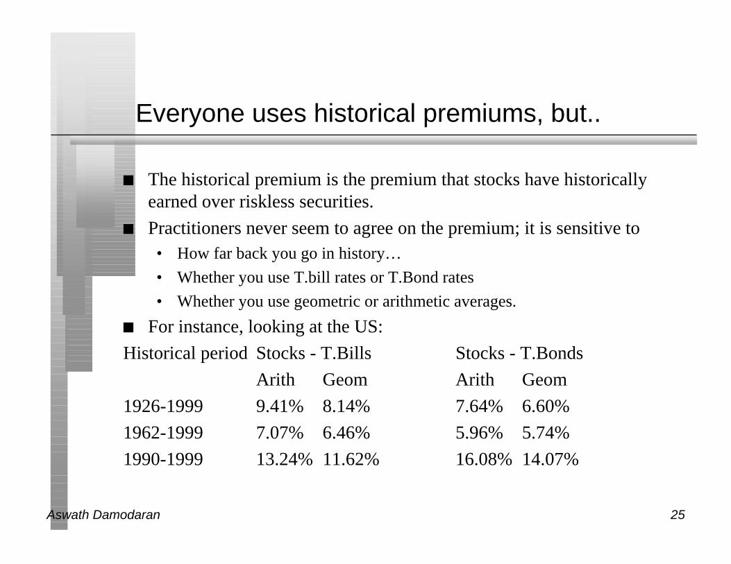
Everyone uses historical premiums, but..
n The historical premium is the premium that stocks have historicallyearned over riskless securities.
n Practitioners never seem to agree on the premium; it is sensitive to• How far back you go in history…
• Whether you use T.bill rates or T.Bond rates
• Whether you use geometric or arithmetic averages.
n For instance, looking at the US:
Historical period Stocks - T.Bills Stocks - T.Bonds
Arith Geom Arith Geom
1926-1999 9.41% 8.14% 7.64% 6.60%
1962-1999 7.07% 6.46% 5.96% 5.74%
1990-1999 13.24% 11.62% 16.08% 14.07%

Aswath Damodaran 26
If you choose to use historical premiums….
n Go back as far as you can. A risk premium comes with a standarderror. Given the annual standard deviation in stock prices is about25%, the standard error in a historical premium estimated over 25years is roughly:
Standard Error in Premium = 25%/√25 = 25%/5 = 5%
n Be consistent in your use of the riskfree rate. Since we argued for longterm bond rates, the premium should be the one over T.Bonds
n Use the geometric risk premium. It is closer to how investors thinkabout risk premiums over long periods.
n Never use historical risk premiums estimated over short periods.
n For emerging markets, start with the base historical premium in the USand add a country spread, based upon the country rating and therelative equity market volatility.

Aswath Damodaran 27
Assessing Country Risk Using CurrencyRatings: Latin America
Country Rating Default Spread over US T.BondArgentina Ba3 525Bolivia B1 600Brazil B2 750Chile Baa1 150Colombia Baa3 200Ecuador B3 850Paraguay B2 750Peru Ba3 525Uruguay Baa3 200Venezuela B2 750

Aswath Damodaran 28
Using Country Ratings to Estimate EquitySpreads
n Country ratings measure default risk. While default risk premiums andequity risk premiums are highly correlated, one would expect equityspreads to be higher than debt spreads.• One way to adjust the country spread upwards is to use information from
the US market. In the US, the equity risk premium has been roughly twicethe default spread on junk bonds.
• Another is to multiply the bond spread by the relative volatility of stockand bond prices in that market. For example,
– Standard Deviation in Merval (Equity) = 42.87%
– Standard Deviation in Argentine Long Bond = 21.37%
– Adjusted Equity Spread = 5.25% (42.87/21.37) = 10.53%

Aswath Damodaran 29
Assessing Country Risk Using CurrencyRatings: Western Europe
Country Rating Default SpreadBelgium Aa1 75Denmark Aaa 0France Aaa 0Germany Aaa 0Greece A2 120Ireland Aaa 0Italy Aa3 90Netherlands Aaa 0Norway Aaa 0Portugal Aa2 85United Kingdom Aaa 0

Aswath Damodaran 30
Using Country Ratings to Estimate EquitySpreads
n Country ratings measure default risk. While default risk premiums andequity risk premiums are highly correlated, one would expect equityspreads to be higher than debt spreads.• One way to adjust the country spread upwards is to use information from
the US market. In the US, the equity risk premium has been roughly twicethe default spread on junk bonds.
• Another is to multiply the bond spread by the relative volatility of stockand bond prices in that market. For example,
– Standard Deviation in MIB30 (Equity) = 15.64%
– Standard Deviation in Italian long bond = 9.2%
– Adjusted Equity Spread = 0.90% (15.64/9.2) = 1.53%

Aswath Damodaran 31
From Country Spreads to Risk premiums
n Approach 1: Assume that every company in the country is equallyexposed to country risk. In this case,
E(Return) = Riskfree Rate + Country Spread + Beta (US premium)Implicitly, this is what you are assuming when you use the local
Government’s dollar borrowing rate as your riskfree rate.
n Approach 2: Assume that a company’s exposure to country risk issimilar to its exposure to other market risk.
E(Return) = Riskfree Rate + Beta (US premium + Country Spread)
n Approach 3: Treat country risk as a separate risk factor and allowfirms to have different exposures to country risk (perhaps based uponthe proportion of their revenues come from non-domestic sales)E(Return)=Riskfree Rate+ β (US premium) + λ (Country Spread)

Aswath Damodaran 32
Estimating Exposure to Country Risk
n Different companies should be exposed to different degrees to countryrisk. For instance, an Italian firm that generates the bulk of its revenuesin Western Europe should be less exposed to country risk in Italy thanone that generates all its business within Italy.
n The factor “λ” measures the relative exposure of a firm to country risk.One simplistic solution would be to do the following:
λ = % of revenues domesticallyfirm/ % of revenues domesticallyavg firm
For instance, if a firm gets 35% of its revenues domestically while theaverage firm in that market gets 70% of its revenues domestically
λ = 35%/ 70 % = 0.5
n There are two implications• A company’s risk exposure is determined by where it does business and
not by where it is located
• Firms might be able to actively manage their country risk exposures

Aswath Damodaran 33
Estimating E(Return) for Siderar: An ArgentineSteel Company
n Assume that the beta for Siderar is 0.71, and that the riskfree rate usedis 6.00%. (US Long Term Bond rate)
n Approach 1: Assume that every company in the country is equallyexposed to country risk. In this case,
E(Return) = 6.00% + 10.53% + 0.71 (5.5%) = 20.44%
n Approach 2: Assume that a company’s exposure to country risk issimilar to its exposure to other market risk.
E(Return) = 6.00% + 0.71 (5.5%+ 10.53%) = 17.38%
n Approach 3: Treat country risk as a separate risk factor and allowfirms to have different exposures to country risk (perhaps based uponthe proportion of their revenues come from non-domestic sales)
E(Return)=6.00% + 0.71(5.5%) + 1.10 (10.53%) = 21.49%
In 1998, Siderar got 76.3% of its revenues from Argentina. The averageacross all Argentinan firms is closer to 70%.

Aswath Damodaran 34
Implied Equity Premiums
n If we use a basic discounted cash flow model, we can estimate theimplied risk premium from the current level of stock prices.
n For instance, if stock prices are determined by a variation of the simpleGordon Growth Model:• Value = Expected Dividends next year/ (Required Returns on Stocks -
Expected Growth Rate)
• Dividends can be extended to included expected stock buybacks.
• Plugging in the current level of the index, the dividends on the index andexpected growth rate will yield a “implied” expected return on stocks.Subtracting out the riskfree rate will yield the implied premium.
n This model can be extended to allow for two stages of growth - aninitial period where the entire market will have earnings growthgreater than that of the economy, and then a stable growth period.

Aswath Damodaran 35
Estimating Implied Premium for U.S. Market:Jan 1, 2000
n Level of the index = 1469
n Treasury bond rate = 6.50%
n Expected Growth rate in earnings (next 5 years) = 10% (Consensusestimate for S&P 500)
n Expected growth rate after year 5 = set equal to T.Bond rate
n Expected dividends + stock buybacks = 1.68% of indexYear 1 Year 2 Year 3 Year 4 Year 5
Expected Dividends = $27.23 $29.95 $32.94 $36.24 $39.86
+ Stock Buybacks
Expected dividends + buybacks in year 6 =39.86 (1.065) = $ 42.45
1469 = 27.23/(1+r) + 29.95/(1+r)2+ + 32.94/(1+r)3 + 36.24/(1+r)4 + (39.86+(42.45/(r-.065))/(1+r)5
Solving for r, r = 8.60%. (Only way to do this is trial and error)
Implied risk premium = 8.60% - 6.50% = 2.10%

Aswath Damodaran 36
Implied Premium for US Equity Market
0.00%
1.00%
2.00%
3.00%
4.00%
5.00%
6.00%
7.00%
Year

Aswath Damodaran 37
Implied Premium for Argentine Market: July 14,1999
n Level of the Index (Merval)= 430.06
n Dividends on the Index = 3.45% of 430.06 (Used weighted yield)
n Other parameters• Riskfree Rate = 6%
• Expected Growth (in nominal dollar terms)– Next 5 years = 12% (Used expected growth rate in Earnings from ADRs)
– After year 5 = 6%
n Solving for the expected return:• Expected return on Equity = 10.81%
• Implied Equity premium = 10.81% - 6.00% = 4.81%

Aswath Damodaran 38
Implied Premium for Italian Market: June 1,1999
n Level of the Index = 35152
n Dividends on the Index = 2.15% of 35152 (Used weighted yield)
n Other parameters• Riskfree Rate = 4.24%
• Expected Growth (in nominal dollar terms)– Next 5 years = 10% (Used expected growth rate in Earnings)
– After year 5 = 5%
n Solving for the expected return:• Expected return on Equity = 7.82%
• Implied Equity premium = 3.58%

Aswath Damodaran 39
Estimating Beta
n The standard procedure for estimating betas is to regress stock returns(Rj) against market returns (Rm) -
Rj = a + b Rm
• where a is the intercept and b is the slope of the regression.
n The slope of the regression corresponds to the beta of the stock, andmeasures the riskiness of the stock.
n This beta has three problems:• It has high standard error
• It reflects the firm’s business mix over the period of the regression, notthe current mix
• It reflects the firm’s average financial leverage over the period rather thanthe current leverage.

Aswath Damodaran 40
Beta Estimation: The Noise Problem

Aswath Damodaran 41
Beta Estimation: The Index Effect

Aswath Damodaran 42
Determinants of Betas
n Product or Service: The beta value for a firm depends upon thesensitivity of the demand for its products and services and of its coststo macroeconomic factors that affect the overall market.• Cyclical companies have higher betas than non-cyclical firms
• Firms which sell more discretionary products will have higher betas thanfirms that sell less discretionary products
n Operating Leverage: The greater the proportion of fixed costs in thecost structure of a business, the higher the beta will be of that business.This is because higher fixed costs increase your exposure to all risk,including market risk.
n Financial Leverage: The more debt a firm takes on, the higher thebeta will be of the equity in that business. Debt creates a fixed cost,interest expenses, that increases exposure to market risk.
Aswath Damodaran 43
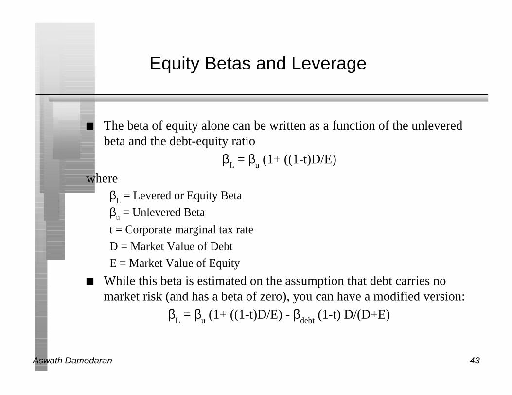
Equity Betas and Leverage
n The beta of equity alone can be written as a function of the unleveredbeta and the debt-equity ratio
βL = βu (1+ ((1-t)D/E)
whereβL = Levered or Equity Beta
βu = Unlevered Beta
t = Corporate marginal tax rate
D = Market Value of Debt
E = Market Value of Equity
n While this beta is estimated on the assumption that debt carries nomarket risk (and has a beta of zero), you can have a modified version:
βL = βu (1+ ((1-t)D/E) - βdebt (1-t) D/(D+E)

Aswath Damodaran 44
Solutions to the Regression Beta Problem
n Modify the regression beta by• changing the index used to estimate the beta
• adjusting the regression beta estimate, by bringing in information aboutthe fundamentals of the company
n Estimate the beta for the firm using• the standard deviation in stock prices instead of a regression against an
index.
• accounting earnings or revenues, which are less noisy than market prices.
n Estimate the beta for the firm from the bottom up without employingthe regression technique. This will require• understanding the business mix of the firm
• estimating the financial leverage of the firm
n Use an alternative measure of market risk that does not need aregression.

Aswath Damodaran 45
Bottom-up Betas
n The bottom up beta can be estimated by :• Taking a weighted (by sales or operating income) average of the
unlevered betas of the different businesses a firm is in.
(The unlevered beta of a business can be estimated by looking at other firms inthe same business)
• Lever up using the firm’s debt/equity ratio
n The bottom up beta will give you a better estimate of the true betawhen• It has lower standard error (SEaverage = SEfirm / √n (n = number of firms)
• It reflects the firm’s current business mix and financial leverage
• It can be estimated for divisions and private firms.
j
j =1
j =k
∑ Operating Income j
Operating IncomeFirm
levered = unlevered 1+ (1− tax rate) (Current Debt/Equity Ratio)[ ]

Aswath Damodaran 46
Bottom-up Beta: Firm in Multiple BusinessesBoeing in 1998
Segment Estimated Value Unlevered Beta Segment Weight
Commercial Aircraft 30,160.48 0.91 70.39%
Defense 12,687.50 0.80 29.61%
Unlevered Beta of firm = 0.91 (.7039) + 0.80 (.2961) = 0.88
Levered Beta CalculationMarket Value of Equity = $ 33,401
Market Value of Debt = $8,143
Market Debt/Equity Ratio = 24.38%
Tax Rate = 35%
Levered Beta for Boeing = 0.88 (1 + (1 - .35) (.2438)) = 1.02

Aswath Damodaran 47
Telecom Italia’s Bottom-up Beta
Business Unlevered D/E Ratio Levered Riskfree Risk Cost of
Beta Beta Rate Premium Equity
Telecom 0.79 18.8% 0.87 4.24% 7.03% 10.36%
Proportion of operating income from telecom = 100%
Unlevered Beta for Telecom Italia= 0.79
Assume now that Telecom Italia decides to go into the internet business,and that the unlevered beta for that business is 1.75. Assuming that25% of Telecom Italia’s business looking forward will come from thisbusiness, what will the firm’s beta be?
Aswath Damodaran 48
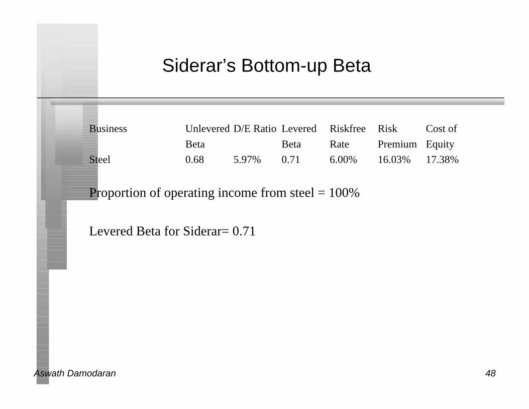
Siderar’s Bottom-up Beta
Business Unlevered D/E Ratio Levered Riskfree Risk Cost of
Beta Beta Rate Premium Equity
Steel 0.68 5.97% 0.71 6.00% 16.03% 17.38%
Proportion of operating income from steel = 100%
Levered Beta for Siderar= 0.71

Aswath Damodaran 49
The Cost of Equity: A Recap
Cost of Equity = Riskfree Rate + Beta * (Risk Premium)
Has to be in the samecurrency as cash flows, and defined in same terms(real or nominal) as thecash flows
Preferably, a bottom-up beta,based upon other firms in thebusiness, and firm’s own financialleverage
Historical Premium1. Mature Equity Market Premium:Average premium earned bystocks over T.Bonds in U.S.2. Country risk premium =Country Default Spread* ( σEquity/σCountry bond)
Implied PremiumBased on how equitymarket is priced todayand a simple valuationmodel
or

Aswath Damodaran 50
Private Business: Owner hasall his wealth invested in thebusiness
Venture Capitalist: Haswealth invested in a numberof companies in one sector
Publicly traded companywith investors who are diversified domesticallyorIPO to investors who aredomestically diversified
Publicly traded companywith investors who are diverisified globallyorIPO to global investors
Market Risk
Int’nl Risk
Sector Risk
Competitive Risk
Project Risk
Market Risk
Int’nl Risk
Sector Risk
Competitive Risk
Project Risk
Market Risk
Int’nl Risk
Sector Risk
Competitive Risk
Project Risk
Market Risk
Int’nl Risk
Sector Risk
Competitive Risk
Project Risk
TotalRisk
Risk added to sectorportfolio
Risk added to domestic portfolio
Risk added to global portfolio
StandardDeviation
Beta relative to sector
Beta relative to local index
Beta relative to global index
40%
25%
15%
10%
100/.4=250
100/.25=400
100/.15=667
100/.10=1000
Investor Type Cares about Risk Measure Cost ofEquity
Firm Value
Valuing a Firm from Different Risk PerspectivesFirm is assumed to have a cash flow of 100 each year forever.

Aswath Damodaran 51
Estimating the Cost of Debt
n The cost of debt is the rate at which you can borrow at currently, Itwill reflect not only your default risk but also the level of interest ratesin the market.
n The two most widely used approaches to estimating cost of debt are:• Looking up the yield to maturity on a straight bond outstanding from the
firm. The limitation of this approach is that very few firms have long termstraight bonds that are liquid and widely traded
• Looking up the rating for the firm and estimating a default spread basedupon the rating. While this approach is more robust, different bonds fromthe same firm can have different ratings. You have to use a median ratingfor the firm
• When in trouble (either because you have no ratings or multiple ratingsfor a firm), estimate a synthetic rating for your firm and the cost of debtbased upon that rating.

Aswath Damodaran 52
Estimating Synthetic Ratings
n The rating for a firm can be estimated using the financialcharacteristics of the firm. In its simplest form, the rating can beestimated from the interest coverage ratio
Interest Coverage Ratio = EBIT / Interest Expenses
n For Siderar, for instance
Interest Coverage Ratio = 161/48 = 3.33• Based upon the relationship between interest coverage ratios and ratings,
we would estimate a rating of A- for Siderar. With a default spread of1.25% (given the rating of A-)
n For Telecom Italia, for instance
Interest Coverage Ratio = 4313/306 = 14.09• Based upon the relationship between interest coverage ratios and ratings,
we would estimate a rating of AAA for Telecom Italia.

Aswath Damodaran 53
Interest Coverage Ratios, Ratings and DefaultSpreads
If Interest Coverage Ratio is Estimated Bond Rating Default Spread
> 8.50 AAA 0.20%
6.50 - 8.50 AA 0.50%
5.50 - 6.50 A+ 0.80%
4.25 - 5.50 A 1.00%
3.00 - 4.25 A– 1.25%
2.50 - 3.00 BBB 1.50%
2.00 - 2.50 BB 2.00%
1.75 - 2.00 B+ 2.50%
1.50 - 1.75 B 3.25%
1.25 - 1.50 B – 4.25%
0.80 - 1.25 CCC 5.00%
0.65 - 0.80 CC 6.00%
0.20 - 0.65 C 7.50%
< 0.20 D 10.00%
Aswath Damodaran 54
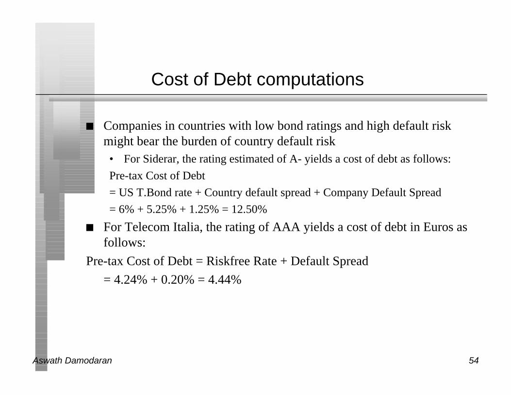
Cost of Debt computations
n Companies in countries with low bond ratings and high default riskmight bear the burden of country default risk• For Siderar, the rating estimated of A- yields a cost of debt as follows:
Pre-tax Cost of Debt
= US T.Bond rate + Country default spread + Company Default Spread
= 6% + 5.25% + 1.25% = 12.50%
n For Telecom Italia, the rating of AAA yields a cost of debt in Euros asfollows:
Pre-tax Cost of Debt = Riskfree Rate + Default Spread
= 4.24% + 0.20% = 4.44%

Aswath Damodaran 55
Synthetic Ratings: Some Caveats
n The relationship between interest coverage ratios and ratings,developed using US companies, tends to travel well, as long as we areanalyzing large manufacturing firms in markets with interest ratesclose to the US interest rate
n They are more problematic when looking at smaller companies inmarkets with higher interest rates than the US.

Aswath Damodaran 56
Weights for the Cost of Capital Computation
n The weights used to compute the cost of capital should be the marketvalue weights for debt and equity.
n There is an element of circularity that is introduced into everyvaluation by doing this, since the values that we attach to the firm andequity at the end of the analysis are different from the values we gavethem at the beginning.
n As a general rule, the debt that you should subtract from firm value toarrive at the value of equity should be the same debt that you used tocompute the cost of capital.

Aswath Damodaran 57
Book Value versus Market Value Weights
n It is also often argued that book values are more reliable than marketvalues since they are not as volatile. Do you agree?
o Yes
o No
n It is often argued that using book value weights is more conservativethan using market value weights. Do you agree?
o Yes
o No

Aswath Damodaran 58
Estimating Cost of Capital: Telecom Italia
n Equity• Cost of Equity = 4.24% + 0.87 (7.03%) = 10.36%
• Market Value of Equity = 9.92* 5255.13 = 52,110 Mil (84.16%)
n Debt• Cost of debt = 4.24% + 0.2% (default spread) = 4.44%
• Market Value of Debt = 9,809 Mil (15.84%)
n Cost of Capital
Cost of Capital = 10.36 % (.8416) + 4.44% (1- .4908) (.1584)) = 9.07%

Aswath Damodaran 59
Telecom Italia: Book Value Weights
n Telecom Italia has a book value of equity of 17,061 million and a bookvalue of debt of 9,809 million. Estimate the cost of capital using bookvalue weights instead of market value weights.
n Is this more conservative?

Aswath Damodaran 60
Estimating Cost of Capital: Siderar
n Equity• Cost of Equity = 6.00% + 0.71 (16.03%) = 17.38%
• Market Value of Equity = 3.20* 310.89 = 995 million (94.37%)
n Debt• Cost of debt = 6.00% + 5.25% (Country default) +1.25% (Company
default) = 12.5%
• Market Value of Debt = 59 Mil (5.63%)
n Cost of Capital
Cost of Capital = 17.38 % (.9437) + 12.50% (1-.3345) (.0563))
= 17.38 % (.9437) + 8.32% (.0563)) = 16.87%

Aswath Damodaran 61
Dealing with Hybrids and Preferred Stock
n When dealing with hybrids (convertible bonds, for instance), break thesecurity down into debt and equity and allocate the amountsaccordingly. Thus, if a firm has $ 125 million in convertible debtoutstanding, break the $125 million into straight debt and conversionoption components. The conversion option is equity.
n When dealing with preferred stock, it is better to keep it as a separatecomponent. The cost of preferred stock is the preferred dividend yield.(As a rule of thumb, if the preferred stock is less than 5% of theoutstanding market value of the firm, lumping it in with debt will makeno significant impact on your valuation).

Aswath Damodaran 62
Recapping the Cost of Capital
Cost of Capital = Cost of Equity (Equity/(Debt + Equity)) + Cost of Borrowing (1-t) (Debt/(Debt + Equity))
Cost of borrowing should be based upon(1) synthetic or actual bond rating(2) default spreadCost of Borrowing = Riskfree rate + Default spread
Marginal tax rate, reflectingtax benefits of debt
Weights should be market value weightsCost of equitybased upon bottom-upbeta

Aswath Damodaran 63
II. Estimating Cash Flows
DCF Valuation

Aswath Damodaran 64
Steps in Cash Flow Estimation
n Estimate the current earnings of the firm• If looking at cash flows to equity, look at earnings after interest expenses -
i.e. net income
• If looking at cash flows to the firm, look at operating earnings after taxes
n Consider how much the firm invested to create future growth• If the investment is not expensed, it will be categorized as capital
expenditures. To the extent that depreciation provides a cash flow, it willcover some of these expenditures.
• Increasing working capital needs are also investments for future growth
n If looking at cash flows to equity, consider the cash flows from netdebt issues (debt issued - debt repaid)

Aswath Damodaran 65
Measuring Cash Flows
Cash flows can be measured to
All claimholders in the firm
EBIT (1- tax rate) - ( Capital Expenditures - Depreciation)- Change in non-cash working capital= Free Cash Flow to Firm (FCFF)
Just Equity Investors
Net Income- (Capital Expenditures - Depreciation)- Change in non-cash Working Capital- (Principal Repaid - New Debt Issues)- Preferred Dividend
Dividends+ Stock Buybacks

Aswath Damodaran 66
Measuring Cash Flow to the Firm
EBIT ( 1 - tax rate)
- (Capital Expenditures - Depreciation)
- Change in Working Capital
= Cash flow to the firm
n Where are the tax savings from interest payments in this cash flow?
Aswath Damodaran 67
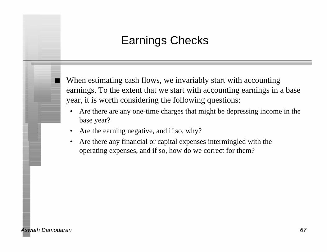
Earnings Checks
n When estimating cash flows, we invariably start with accountingearnings. To the extent that we start with accounting earnings in a baseyear, it is worth considering the following questions:• Are there are any one-time charges that might be depressing income in the
base year?
• Are the earning negative, and if so, why?
• Are there any financial or capital expenses intermingled with theoperating expenses, and if so, how do we correct for them?
Aswath Damodaran 68
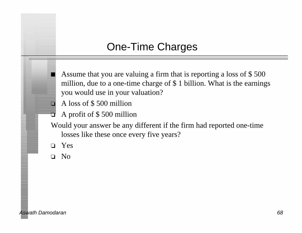
One-Time Charges
n Assume that you are valuing a firm that is reporting a loss of $ 500million, due to a one-time charge of $ 1 billion. What is the earningsyou would use in your valuation?
o A loss of $ 500 million
o A profit of $ 500 million
Would your answer be any different if the firm had reported one-timelosses like these once every five years?
o Yes
o No

Aswath Damodaran 69
To get earnings right...
n We need to normalize earnings, if the base year earnings are negativeor abnormally low
n We need to adjust earnings to reflect the effects of the accountingtreatment of• Some financing expenses as operating expenses
• Some capital expenses as operating expenses

Aswath Damodaran 70
Negative Earnings: Why they are a problem
n When earnings are negative, you cannot start with that number in thebase year and expect to grow yourself out of the problem.
n The key to valuation, when earnings are negative, is to some how workwith the numbers until the earnings become positive. Exactly how thisis done will depend upon why the earnings are negative in the firstplace.
n In fact, this applies even if your earnings are positive but lower thannormal.

Aswath Damodaran 71
A Framework for Dealing with NegativeEarnings
A Framework for Analyzing Companies with Negative or Abnormally Low Earnings
Why are the earnings negative or abnormally low?
TemporaryProblems
Cyclicality:Eg. Auto firmin recession
StructuralProblems: Eg. Cable co. with high infrastruccture investments.
LeverageProblems: Eg. An otherwise healthy firm with too much debt.
Long-termOperatingProblems: Eg. A firm with significant production or cost problems.
Normalize Earnings
Value the firm by doing detailed cash flow forecasts starting with revenues and reduce or eliminate the problem over time.:(a) If problem is structural: Target for operating margins of stable firms in the sector.(b) If problem is leverage : Target for a debt ratio that the firm will be comfortable with by end of period, which could be its own optimal or the industry average.(c) If problem is operating : Target for an industry-average operating margin.
If firm’s size has notchanged significantlyover time
Average DollarEarnings (Net Income if Equity and EBIT if Firm made bythe firm over time
If firm’s size has changedover time
Use firm’s average ROE (if valuing equity) or average ROC (if valuing firm) on current BV of equity (if ROE) or current BV of capital (if ROC)

Aswath Damodaran 72
Correcting Accounting Earnings
n The Operating Lease Adjustment: While accounting convention treatsoperating leases as operating expenses, they are really financialexpenses and need to be reclassified as such. This has no effect onequity earnings but does change the operating earnings
n The R & D Adjustment: Since R&D is a capital expenditure (ratherthan an operating expense), the operating income has to be adjusted toreflect its treatment.
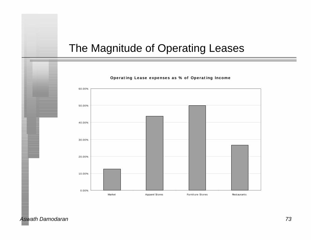
Aswath Damodaran 73
The Magnitude of Operating Leases
Operating Lease expenses as % of Operating Income
0.00%
10.00%
20.00%
30.00%
40.00%
50.00%
60.00%
Market Apparel Stores Furniture Stores Restaurants

Aswath Damodaran 74
Dealing with Operating Lease Expenses
n Operating Lease Expenses are treated as operating expenses incomputing operating income. In reality, operating lease expensesshould be treated as financing expenses, with the followingadjustments to earnings and capital:
n Debt Value of Operating Leases = PV of Operating Lease Expenses atthe pre-tax cost of debt
n Adjusted Operating Earnings = Operating Earnings + Pre-tax cost ofDebt * PV of Operating Leases.

Aswath Damodaran 75
Operating Leases at The Home Depot in 1998
n The pre-tax cost of debt at the Home Depot is 6.25%Yr Operating Lease Expense Present Value 1 $ 294 $ 277 2 $ 291 $ 258 3 $ 264 $ 220 4 $ 245 $ 192 5 $ 236 $ 174 6-15 $ 270 $ 1,450 (PV of 10-yr annuity)
Present Value of Operating Leases =$ 2,571
n Debt outstanding at the Home Depot = $1,205 + $2,571 = $3,776 mil(The Home Depot has other debt outstanding of $1,205 million)
n Adjusted Operating Income = $2,016 + 2,571 (.0625) = $2,177 mil

Aswath Damodaran 76
The Effects of Capitalizing Operating Leases
n Debt : will increase, leading to an increase in debt ratios used in thecost of capital and levered beta calculation
n Operating income: will increase, since operating leases will now bebefore the imputed interest on the operating lease expense
n Net income: will be unaffected since it is after both operating andfinancial expenses anyway
n Return on Capital will generally decrease since the increase inoperating income will be proportionately lower than the increase inbook capital invested

Aswath Damodaran 77
The Magnitude of R&D Expenses
R&D as % of Operating Income
0.00%
10.00%
20.00%
30.00%
40.00%
50.00%
60.00%
Market Petroleum Computers

Aswath Damodaran 78
R&D Expenses: Operating or Capital Expenses
n Accounting standards require us to consider R&D as an operatingexpense even though it is designed to generate future growth. It ismore logical to treat it as capital expenditures.
n To capitalize R&D,• Specify an amortizable life for R&D (2 - 10 years)
• Collect past R&D expenses for as long as the amortizable life
• Sum up the unamortized R&D over the period. (Thus, if the amortizablelife is 5 years, the research asset can be obtained by adding up 1/5th of theR&D expense from five years ago, 2/5th of the R&D expense from fouryears ago...:

Aswath Damodaran 79
Capitalizing R&D Expenses: Bristol Myers
n R & D was assumed to have a 10-year life.Year R&D Expense Unamortized portion Amortization this year
-1 1385.00 1.00 1385.00 138.50
-2 1276.00 0.90 1148.40 127.60
-3 1199.00 0.80 959.20 119.90
-4 1108.00 0.70 775.60 110.80
-5 1128.00 0.60 676.80 112.80
-6 1083.00 0.50 541.50 108.30
-7 983.00 0.40 393.20 98.30
-8 881.00 0.30 264.30 88.10
-9 789.00 0.20 157.80 78.90
-10 688.00 0.10 68.80 68.80
Sum = $6,370.60 1052.00
Value of research asset = $ 6,371 million
Amortization of research asset in 1998 = $ 1,052 million
Adjustment to Operating Income = $ 1,385 million - $ 1,052 million =$ 333 million

Aswath Damodaran 80
The Effect of Capitalizing R&D
n Operating Income will generally increase, though it depends uponwhether R&D is growing or not. If it is flat, there will be no effectsince the amortization will offset the R&D added back. The fasterR&D is growing the more operating income will be affected.
n Net income will increase proportionately, depending again upon howfast R&D is growing
n Book value of equity (and capital) will increase by the capitalizedResearch asset
n Capital expenditures will increase by the amount of R&D;Depreciation will increase by the amortization of the research asset;For all firms, the net cap ex will increase by the same amount as theafter-tax operating income.

Aswath Damodaran 81
What tax rate?
n The tax rate that you should use in computing the after-tax operatingincome should be
o The effective tax rate in the financial statements (taxes paid/Taxableincome)
o The tax rate based upon taxes paid and EBIT (taxes paid/EBIT)
o The marginal tax rate
o None of the above
o Any of the above, as long as you compute your after-tax cost of debtusing the same tax rate

Aswath Damodaran 82
The Right Tax Rate to Use
n The choice really is between the effective and the marginal tax rate. Indoing projections, it is far safer to use the marginal tax rate since theeffective tax rate is really a reflection of the difference between theaccounting and the tax books.
n By using the marginal tax rate, we tend to understate the after-taxoperating income in the earlier years, but the after-tax tax operatingincome is more accurate in later years
n If you choose to use the effective tax rate, adjust the tax rate towardsthe marginal tax rate over time.
n The tax rate used to compute the after-tax cost of debt has to be themarginal tax rate, and can be different from the tax rate used tocompute after-tax operating income.

Aswath Damodaran 83
A Tax Rate for a Money Losing Firm
n Assume that you are trying to estimate the after-tax operating incomefor a firm with $ 1 billion in net operating losses carried forward. Thisfirm is expected to have operating income of $ 500 million each yearfor the next 3 years, and the marginal tax rate on income for all firmsthat make money is 40%. Estimate the after-tax operating income eachyear for the next 3 years.
Year 1 Year 2 Year 3
EBIT 500 500 500
Taxes
EBIT (1-t)
Tax rate

Aswath Damodaran 84
Net Capital Expenditures
n Net capital expenditures represent the difference between capitalexpenditures and depreciation. Depreciation is a cash inflow that paysfor some or a lot (or sometimes all of) the capital expenditures.
n In general, the net capital expenditures will be a function of how fast afirm is growing or expecting to grow. High growth firms will havemuch higher net capital expenditures than low growth firms.
n Assumptions about net capital expenditures can therefore never bemade independently of assumptions about growth in the future.
Aswath Damodaran 85
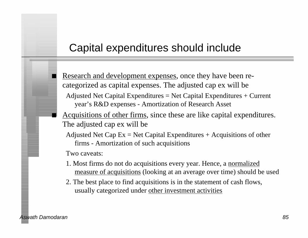
Capital expenditures should include
n Research and development expenses, once they have been re-categorized as capital expenses. The adjusted cap ex will beAdjusted Net Capital Expenditures = Net Capital Expenditures + Current
year’s R&D expenses - Amortization of Research Asset
n Acquisitions of other firms, since these are like capital expenditures.The adjusted cap ex will beAdjusted Net Cap Ex = Net Capital Expenditures + Acquisitions of other
firms - Amortization of such acquisitions
Two caveats:
1. Most firms do not do acquisitions every year. Hence, a normalizedmeasure of acquisitions (looking at an average over time) should be used
2. The best place to find acquisitions is in the statement of cash flows,usually categorized under other investment activities
Aswath Damodaran 86
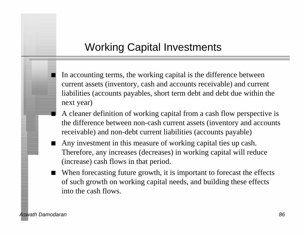
Working Capital Investments
n In accounting terms, the working capital is the difference betweencurrent assets (inventory, cash and accounts receivable) and currentliabilities (accounts payables, short term debt and debt due within thenext year)
n A cleaner definition of working capital from a cash flow perspective isthe difference between non-cash current assets (inventory and accountsreceivable) and non-debt current liabilities (accounts payable)
n Any investment in this measure of working capital ties up cash.Therefore, any increases (decreases) in working capital will reduce(increase) cash flows in that period.
n When forecasting future growth, it is important to forecast the effectsof such growth on working capital needs, and building these effectsinto the cash flows.

Aswath Damodaran 87
Working Capital: General Propositions
n Changes in non-cash working capital from year to year tend to bevolatile. A far better estimate of non-cash working capital needs,looking forward, can be estimated by looking at non-cash workingcapital as a proportion of revenues
n Some firms have negative non-cash working capital. Assuming thatthis will continue into the future will generate positive cash flows forthe firm. While this is indeed feasible for a period of time, it is notforever. Thus, it is better that non-cash working capital needs be set tozero, when it is negative.

Aswath Damodaran 88
Dividends and Cash Flows to Equity
n In the strictest sense, the only cash flow that an investor will receivefrom an equity investment in a publicly traded firm is the dividend thatwill be paid on the stock.
n Actual dividends, however, are set by the managers of the firm andmay be much lower than the potential dividends (that could have beenpaid out)• managers are conservative and try to smooth out dividends
• managers like to hold on to cash to meet unforeseen future contingenciesand investment opportunities
n When actual dividends are less than potential dividends, using a modelthat focuses only on dividends will under state the true value of theequity in a firm.

Aswath Damodaran 89
Measuring Potential Dividends
n Some analysts assume that the earnings of a firm represent its potentialdividends. This cannot be true for several reasons:• Earnings are not cash flows, since there are both non-cash revenues and
expenses in the earnings calculation
• Even if earnings were cash flows, a firm that paid its earnings out asdividends would not be investing in new assets and thus could not grow
• Valuation models, where earnings are discounted back to the present, willover estimate the value of the equity in the firm
n The potential dividends of a firm are the cash flows left over after thefirm has made any “investments” it needs to make to create futuregrowth and net debt repayments (debt repayments - new debt issues)• The common categorization of capital expenditures into discretionary and
non-discretionary loses its basis when there is future growth built into thevaluation.

Aswath Damodaran 90
Estimating Cash Flows: FCFE
n Cash flows to Equity for a Levered FirmNet Income
- (Capital Expenditures - Depreciation)
- Changes in non-cash Working Capital
- (Principal Repayments - New Debt Issues)
= Free Cash flow to Equity
• I have ignored preferred dividends. If preferred stock exist, preferreddividends will also need to be netted out

Aswath Damodaran 91
Estimating FCFE when Leverage is Stable
Net Income
- (1- δ) (Capital Expenditures - Depreciation)
- (1- δ) Working Capital Needs
= Free Cash flow to Equity
δ = Debt/Capital Ratio
For this firm,• Proceeds from new debt issues = Principal Repayments + d (Capital
Expenditures - Depreciation + Working Capital Needs)
n In computing FCFE, the book value debt to capital ratio should beused when looking back in time but can be replaced with the marketvalue debt to capital ratio, looking forward.

Aswath Damodaran 92
Estimating FCFE: Disney
n Net Income=$ 1533 Million
n Capital spending = $ 1,746 Million
n Depreciation per Share = $ 1,134 Million
n Non-cash Working capital Change = $ 477 Million
n Debt to Capital Ratio = 23.83%
n Estimating FCFE (1997):Net Income $1,533 Mil
- (Cap. Exp - Depr)*(1-DR) $465.90
Chg. Working Capital*(1-DR) $363.33
= Free CF to Equity $ 704 Million
Dividends Paid $ 345 Million

Aswath Damodaran 93
FCFE and Leverage: Is this a free lunch?
Debt Ratio and FCFE: Disney
0
200
400
600
800
1000
1200
1400
1600
0% 10% 20% 30% 40% 50% 60% 70% 80% 90%
Debt Ratio
FCFE

Aswath Damodaran 94
FCFE and Leverage: The Other Shoe Drops
Debt Ratio and Beta
0.00
1.00
2.00
3.00
4.00
5.00
6.00
7.00
8.00
0% 10% 20% 30% 40% 50% 60% 70% 80% 90%
Debt Ratio
Beta

Aswath Damodaran 95
Leverage, FCFE and Value
n In a discounted cash flow model, increasing the debt/equity ratio willgenerally increase the expected free cash flows to equity investors overfuture time periods and also the cost of equity applied in discountingthese cash flows. Which of the following statements relating leverageto value would you subscribe to?
o Increasing leverage will increase value because the cash flow effectswill dominate the discount rate effects
o Increasing leverage will decrease value because the risk effect will begreater than the cash flow effects
o Increasing leverage will not affect value because the risk effect willexactly offset the cash flow effect
o Any of the above, depending upon what company you are looking atand where it is in terms of current leverage

Aswath Damodaran 96
Estimating FCFE: Brahma
n Net Income (1996) = 325 Million BR
n Capital spending (1996) = 396 Million
n Depreciation (1996) = 183 Million BR
n Non-cash Working capital Change (1996) = 12 Million BR
n Debt Ratio = 43.48%
n Estimating FCFE (1996):Earnings per Share 325.00 Million BR
- (Cap Ex-Depr) (1-DR) = (396-183)(1-.4348) = 120.39 Million BR
- Change in Non-cash WC (1-DR) = 12 (1-.4348) = 6.78 Million BR
Free Cashflow to Equity 197.83 Million Br
Dividends Paid 232.00 Million BR

Aswath Damodaran 97
III. Estimating Growth
DCF Valuation

Aswath Damodaran 98
Ways of Estimating Growth in Earnings
n Look at the past• The historical growth in earnings per share is usually a good starting point
for growth estimation
n Look at what others are estimating• Analysts estimate growth in earnings per share for many firms. It is useful
to know what their estimates are.
n Look at fundamentals• Ultimately, all growth in earnings can be traced to two fundamentals -
how much the firm is investing in new projects, and what returns theseprojects are making for the firm.

Aswath Damodaran 99
I. Historical Growth in EPS
n Historical growth rates can be estimated in a number of different ways• Arithmetic versus Geometric Averages
• Simple versus Regression Models
n Historical growth rates can be sensitive to• the period used in the estimation
n In using historical growth rates, the following factors have to beconsidered• how to deal with negative earnings
• the effect of changing size

Aswath Damodaran 100
Disney: Arithmetic versus Geometric GrowthRates
Year EPS Growth Rate
1990 1.50
1991 1.20 -20.00%
1992 1.52 26.67%
1993 1.63 7.24%
1994 2.04 25.15%
1995 2.53 24.02%
1996 2.23 -11.86%
Arithmetic Average = 8.54%
Geometric Average = (2.23/1.50) (1/6) – 1 = 6.83% (6 years of growth)
n The arithmetic average will be higher than the geometric average rate
n The difference will increase with the standard deviation in earnings

Aswath Damodaran 101
Disney: The Effects of Altering EstimationPeriods
Year EPS Growth Rate
1991 1.20
1992 1.52 26.67%
1993 1.63 7.24%
1994 2.04 25.15%
1995 2.53 24.02%
1996 2.23 -11.86%
Taking out 1990 from our sample, changes the growth rates materially:
Arithmetic Average from 1991 to 1996 = 14.24%
Geometric Average = (2.23/1.20)(1/5) = 13.19% (5 years of growth)

Aswath Damodaran 102
Disney: Linear and Log-Linear Models forGrowth
Year Year Number EPS ln(EPS)
1990 1 $ 1.50 0.4055
1991 2 $ 1.20 0.1823
1992 3 $ 1.52 0.4187
1993 4 $ 1.63 0.4886
1994 5 $ 2.04 0.7129
1995 6 $ 2.53 0.9282
1996 7 $ 2.23 0.8020
n EPS = 1.04 + 0.19 ( t): EPS grows by $0.19 a year
Growth Rate = $0.19/$1.81 = 10.5% ($1.81: Average EPS from 90-96)
n ln(EPS) = 0.1375 + 0.1063 (t): Growth rate approximately 10.63%

Aswath Damodaran 103
A Test
n You are trying to estimate the growth rate in earnings per share atTime Warner from 1996 to 1997. In 1996, the earnings per share was adeficit of $0.05. In 1997, the expected earnings per share is $ 0.25.What is the growth rate?
o -600%
o +600%
o +120%
o Cannot be estimated

Aswath Damodaran 104
Dealing with Negative Earnings
n When the earnings in the starting period are negative, the growth ratecannot be estimated. (0.30/-0.05 = -600%)
n There are three solutions:• Use the higher of the two numbers as the denominator (0.30/0.25 = 120%)
• Use the absolute value of earnings in the starting period as thedenominator (0.30/0.05=600%)
• Use a linear regression model and divide the coefficient by the averageearnings.
n When earnings are negative, the growth rate is meaningless. Thus,while the growth rate can be estimated, it does not tell you much aboutthe future.

Aswath Damodaran 105
The Effect of Size on Growth: Callaway Golf
Year Net Profit Growth Rate
1990 1.80
1991 6.40 255.56%
1992 19.30 201.56%
1993 41.20 113.47%
1994 78.00 89.32%
1995 97.70 25.26%
1996 122.30 25.18%
Geometric Average Growth Rate = 102%

Aswath Damodaran 106
Extrapolation and its Dangers
Year Net Profit
1996 $ 122.30
1997 $ 247.05
1998 $ 499.03
1999 $ 1,008.05
2000 $ 2,036.25
2001 $ 4,113.23
n If net profit continues to grow at the same rate as it has in the past 6years, the expected net income in 5 years will be $ 4.113 billion.

Aswath Damodaran 107
II. Analyst Forecasts of Growth
n While the job of an analyst is to find under and over valued stocks inthe sectors that they follow, a significant proportion of an analyst’stime (outside of selling) is spent forecasting earnings per share.• Most of this time, in turn, is spent forecasting earnings per share in the
next earnings report
• While many analysts forecast expected growth in earnings per share overthe next 5 years, the analysis and information (generally) that goes intothis estimate is far more limited.
n Analyst forecasts of earnings per share and expected growth arewidely disseminated by services such as Zacks and IBES, at least forU.S companies.

Aswath Damodaran 108
How good are analysts at forecasting growth?
n Analysts forecasts of EPS tend to be closer to the actual EPS thansimple time series models, but the differences tend to be small
Study Time Period Analyst Forecast Error Time Series Model
Collins & Hopwood Value Line Forecasts 31.7% 34.1%
1970-74
Brown & Rozeff Value Line Forecasts 28.4% 32.2%
1972-75
Fried & Givoly Earnings Forecaster 16.4% 19.8%
1969-79
n The advantage that analysts have over time series models• tends to decrease with the forecast period (next quarter versus 5 years)
• tends to be greater for larger firms than for smaller firms
• tends to be greater at the industry level than at the company level
n Forecasts of growth (and revisions thereof) tend to be highly correlatedacross analysts.

Aswath Damodaran 109
Are some analysts more equal than others?
n A study of All-America Analysts (chosen by Institutional Investor)found that• There is no evidence that analysts who are chosen for the All-America
Analyst team were chosen because they were better forecasters ofearnings. (Their median forecast error in the quarter prior to being chosenwas 30%; the median forecast error of other analysts was 28%)
• However, in the calendar year following being chosen as All-Americaanalysts, these analysts become slightly better forecasters than their lessfortunate brethren. (The median forecast error for All-America analysts is2% lower than the median forecast error for other analysts)
• Earnings revisions made by All-America analysts tend to have a muchgreater impact on the stock price than revisions from other analysts
• The recommendations made by the All America analysts have a greaterimpact on stock prices (3% on buys; 4.7% on sells). For theserecommendations the price changes are sustained, and they continue torise in the following period (2.4% for buys; 13.8% for the sells).

Aswath Damodaran 110
The Five Deadly Sins of an Analyst
n Tunnel Vision: Becoming so focused on the sector and valuationswithin the sector that they lose sight of the bigger picture.
n Lemmingitis:Strong urge felt by analysts to change recommendations& revise earnings estimates when other analysts do the same.
n Stockholm Syndrome(shortly to be renamed the Bre-X syndrome):Refers to analysts who start identifying with the managers of the firmsthat they are supposed to follow.
n Factophobia (generally is coupled with delusions of being a famousstory teller): Tendency to base a recommendation on a “story” coupledwith a refusal to face the facts.
n Dr. Jekyll/Mr.Hyde: Analyst who thinks his primary job is to bring ininvestment banking business to the firm.

Aswath Damodaran 111
Propositions about Analyst Growth Rates
n Proposition 1: There if far less private information and far morepublic information in most analyst forecasts than is generally claimed.
n Proposition 2: The biggest source of private information for analystsremains the company itself which might explain• why there are more buy recommendations than sell recommendations
(information bias and the need to preserve sources)
• why there is such a high correlation across analysts forecasts and revisions
• why All-America analysts become better forecasters than other analystsafter they are chosen to be part of the team.
n Proposition 3: There is value to knowing what analysts are forecastingas earnings growth for a firm. There is, however, danger when theyagree too much (lemmingitis) and when they agree to little (in whichcase the information that they have is so noisy as to be useless).

Aswath Damodaran 112
III. Fundamental Growth Rates
Investmentin ExistingProjects$ 1000
Current Return onInvestment on Projects12%
X =CurrentEarnings$120
Investmentin ExistingProjects$1000
Next Period’s Return onInvestment12%
XInvestmentin NewProjects$100
Return onInvestment onNew Projects12%
X+ =Next Period’sEarnings132
Investmentin ExistingProjects$1000
Change inROI from current to nextperiod: 0%
XInvestmentin NewProjects$100
Return onInvestment onNew Projects12%
X+ Change in Earnings$ 12=
Aswath Damodaran 113
Growth Rate Derivations
In the special case where ROI on existing projects remains unchanged and is equal to the ROI on new projects
Investment in New Projects
Current EarningsReturn on Investment
Change in Earnings
Current Earnings=X
Reinvestment Rate X Return on Investment = Growth Rate in Earnings
in the more general case where ROI can change from period to period, this can be expanded as follows:
Investment in Existing Projects*(Change in ROI) + New Projects (ROI)
Investment in Existing Projects* Current ROIChange in Earnings
Current Earnings=
100
120 X 12% =$12
$120
For instance, if the ROI increases from 12% to 13%, the expected growth rate can be written as follows:
83.33% X 12% = 10%
$1,000 * (.13 - .12) + 100 (13%)
$ 1000 * .12$23
$120= = 19.17%

Aswath Damodaran 114
Expected Long Term Growth in EPS
n When looking at growth in earnings per share, these inputs can be cast asfollows:
Reinvestment Rate = Retained Earnings/ Current Earnings = Retention RatioReturn on Investment = ROE = Net Income/Book Value of Equity
n In the special case where the current ROE is expected to remain unchangedgEPS = Retained Earningst-1/ NIt-1 * ROE
= Retention Ratio * ROE= b * ROE
n Proposition 1: The expected growth rate in earnings for a companycannot exceed its return on equity in the long term.

Aswath Damodaran 115
Estimating Expected Growth in EPS: ABNAmro
n Current Return on Equity = 15.79%
n Current Retention Ratio = 1 - DPS/EPS = 1 - 1.13/2.45 = 53.88%
n If ABN Amro can maintain its current ROE and retention ratio, itsexpected growth in EPS will be:
Expected Growth Rate = 0.5388 (15.79%) = 8.51%

Aswath Damodaran 116
Expected ROE changes and Growth
n Assume now that ABN Amro’s ROE next year is expected to increaseto 17%, while its retention ratio remains at 53.88%. What is the newexpected long term growth rate in earnings per share?
n Will the expected growth rate in earnings per share next year begreater than, less than or equal to this estimate?
o greater than
o less than
o equal to

Aswath Damodaran 117
Changes in ROE and Expected Growth
n When the ROE is expected to change,gEPS= b *ROEt+1 +(ROEt+1– ROEt) ROEt
n Proposition 2: Small changes in ROE translate into large changes inthe expected growth rate.• The lower the current ROE, the greater the effect on growth of changes in
the ROE.
n Proposition 3: No firm can, in the long term, sustain growth inearnings per share from improvement in ROE.• Corollary: The higher the existing ROE of the company (relative to the
business in which it operates) and the more competitive the business inwhich it operates, the smaller the scope for improvement in ROE.

Aswath Damodaran 118
Changes in ROE: ABN Amro
n Assume now that ABN’s expansion into Asia will push up the ROE to17%, while the retention ratio will remain 53.88%. The expectedgrowth rate in that year will be:
gEPS= b *ROEt+1 + (ROEt+1– ROEt)(BV of Equityt )/ ROEt (BV of Equityt)=(.5388)(.17)+(.17-.1579)/(.1579)= 16.83%
n Note that 1.21% improvement in ROE translates into amost a doublingof the growth rate from 8.51% to 16.83%.

Aswath Damodaran 119
ROE and Leverage
n ROE = ROC + D/E (ROC - i (1-t))
where,
ROC = (Net Income + Interest (1 - tax rate)) / BV of Capital
= EBIT (1- t) / BV of Capital
D/E = BV of Debt/ BV of Equity
i = Interest Expense on Debt / BV of Debt
t = Tax rate on ordinary income
n Note that BV of capital = BV of Debt + BV of Equity.

Aswath Damodaran 120
Decomposing ROE: Brahma
n Real Return on Capital = 687 (1-.32) / (1326+542+478) = 19.91%• This is assumed to be real because both the book value and income are
inflation adjusted.
n Debt/Equity Ratio = (542+478)/1326 = 0.77
n After-tax Cost of Debt = 8.25% (1-.32) = 5.61% (Real BR)
n Return on Equity = ROC + D/E (ROC - i(1-t))19.91% + 0.77 (19.91% - 5.61%) = 30.92%

Aswath Damodaran 121
Decomposing ROE: Titan Watches
n Return on Capital = 713 (1-.25)/(1925+2378+1303) = 9.54%
n Debt/Equity Ratio = (2378 + 1303)/1925 = 1.91
n After-tax Cost of Debt = 13.5% (1-.25) = 10.125%
n Return on Equity = ROC + D/E (ROC - i(1-t))9.54% + 1.91 (9.54% - 10.125%) = 8.42%

Aswath Damodaran 122
Expected Growth in EBIT And Fundamentals
n When looking at growth in operating income, the definitions areReinvestment Rate = (Net Capital Expenditures + Change in WC)/EBIT(1-t)
Return on Investment = ROC = EBIT(1-t)/(BV of Debt + BV of Equity)
n Reinvestment Rate and Return on Capital
gEBIT = (Net Capital Expenditures + Change in WC)/EBIT(1-t) * ROC= Reinvestment Rate * ROC
n Proposition: No firm can expect its operating income to grow overtime without reinvesting some of the operating income in net capitalexpenditures and/or working capital.
n Proposition: The net capital expenditure needs of a firm, for a givengrowth rate, should be inversely proportional to the quality of itsinvestments.

Aswath Damodaran 123
No Net Capital Expenditures and Long TermGrowth
n You are looking at a valuation, where the terminal value is based uponthe assumption that operating income will grow 3% a year forever, butthere are no net cap ex or working capital investments being madeafter the terminal year. When you confront the analyst, he contendsthat this is still feasible because the company is becoming moreefficient with its existing assets and can be expected to increase itsreturn on capital over time. Is this a reasonable explanation?
o Yes
o No
n Explain.

Aswath Damodaran 124
Estimating Growth in EBIT: Disney
n Reinvestment Rate = 50%
n Return on Capital =18.69%
n Expected Growth in EBIT =.5(18.69%) = 9.35%

Aswath Damodaran 125
Estimating Growth in EBIT: Hansol Paper
n Net Capital Expenditures = (150,000-45000) = 105,000 Million WN
(I normalized capital expenditures to account for lumpy investments)
n Change in Working Capital = 1000 Million WN
n Reinvestment Rate = (105,000+1,000)/(109,569*.7) = 138.20%
n Return on Capital = 6.76%
n Expected Growth in EBIT = 6.76% (1.382) = 9.35%

Aswath Damodaran 126
A Profit Margin View of Growth
n The relationship between growth and return on investment can also beframed in terms of profit margins:
n In the case of growth in EPS
Growth in EPS = Retention Ratio * ROE
= Retention Ratio*Net Income/Sales * Sales/BV of Equity
= Retention Ratio * Net Margin * Equity Turnover Ratio
Growth in EBIT = Reinvestment Rate * ROC
= Reinvestment Rate * EBIT(1-t)/ BV of Capital
= Reinvestment Rate * AT Operating Margin * Capital Turnover Ratio
Aswath Damodaran 127
IV. Growth Patterns
Discounted Cashflow Valuation

Aswath Damodaran 128
Stable Growth and Terminal Value
n When a firm’s cash flows grow at a “constant” rate forever, the presentvalue of those cash flows can be written as:Value = Expected Cash Flow Next Period / (r - g)
where,
r = Discount rate (Cost of Equity or Cost of Capital)
g = Expected growth rate
n This “constant” growth rate is called a stable growth rate and cannotbe higher than the growth rate of the economy in which the firmoperates.
n While companies can maintain high growth rates for extended periods,they will all approach “stable growth” at some point in time.
n When they do approach stable growth, the valuation formula abovecan be used to estimate the “terminal value” of all cash flows beyond.

Aswath Damodaran 129
Growth Patterns
n A key assumption in all discounted cash flow models is the period ofhigh growth, and the pattern of growth during that period. In general,we can make one of three assumptions:• there is no high growth, in which case the firm is already in stable growth
• there will be high growth for a period, at the end of which the growth ratewill drop to the stable growth rate (2-stage)
• there will be high growth for a period, at the end of which the growth ratewill decline gradually to a stable growth rate(3-stage)
Stable Growth 2-Stage Growth 3-Stage Growth

Aswath Damodaran 130
Determinants of Growth Patterns
n Size of the firm• Success usually makes a firm larger. As firms become larger, it becomes
much more difficult for them to maintain high growth rates
n Current growth rate• While past growth is not always a reliable indicator of future growth,
there is a correlation between current growth and future growth. Thus, afirm growing at 30% currently probably has higher growth and a longerexpected growth period than one growing 10% a year now.
n Barriers to entry and differential advantages• Ultimately, high growth comes from high project returns, which, in turn,
comes from barriers to entry and differential advantages.
• The question of how long growth will last and how high it will be cantherefore be framed as a question about what the barriers to entry are, howlong they will stay up and how strong they will remain.

Aswath Damodaran 131
Stable Growth and Fundamentals
n The growth rate of a firm is driven by its fundamentals - how much itreinvests and how high project returns are. As growth rates approach“stability”, the firm should be given the characteristics of a stablegrowth firm.
Model High Growth Firms usually Stable growth firms usually
DDM 1. Pay no or low dividends 1. Pay high dividends
2. Have high risk 2. Have average risk
3. Earn high ROC 3. Earn ROC closer to WACC
FCFE/ 1. Have high net cap ex 1. Have lower net cap ex
FCFF 2. Have high risk 2. Have average risk
3. Earn high ROC 3. Earn ROC closer to WACC
4. Have low leverage 4. Have leverage closer to industry average

Aswath Damodaran 132
The Dividend Discount Model: EstimatingStable Growth Inputs
n Consider the example of ABN Amro. Based upon its current return onequity of 15.79% and its retention ratio of 53.88%, we estimated agrowth in earnings per share of 8.51%.
n Let us assume that ABN Amro will be in stable growth in 5 years. Atthat point, let us assume that its return on equity will be closer to theaverage for European banks of 15%, and that it will grow at a nominalrate of 5% (Real Growth + Inflation Rate in NV)
n The expected payout ratio in stable growth can then be estimated asfollows:
Stable Growth Payout Ratio = 1 - g/ ROE = 1 - .05/.15 = 66.67%g = b (ROE)
b = g/ROE
Payout = 1- b

Aswath Damodaran 133
The FCFE/FCFF Models: Estimating StableGrowth Inputs
n To estimate the net capital expenditures in stable growth, consider thegrowth in operating income that we assumed for Disney. Thereinvestment rate was assumed to be 50%, and the return on capitalwas assumed to be 18.69%, giving us an expected growth rate of9.35%.
n In stable growth (which will occur 10 years from now), assume thatDisney will have a return on capital of 16%, and that its operatingincome is expected to grow 5% a year forever.
Reinvestment Rate = Growth in Operating Income/ROC = 5/16
n This reinvestment rate includes both net cap ex and working capital.
Estimated EBIT (1-t) in year 11 = $ 9,098 Million
Reinvestment = $9,098(5/16) = $2,843 Million
Net Capital Expenditures = Reinvestment - Change in Working Capital11
= $ 2,843m -105m = 2,738m

Aswath Damodaran 134
V. Beyond Inputs: Choosing andUsing the Right Model
Discounted Cashflow Valuation

Aswath Damodaran 135
Summarizing the Inputs
n In summary, at this stage in the process, we should have an estimate ofthe• the current cash flows on the investment, either to equity investors
(dividends or free cash flows to equity) or to the firm (cash flow to thefirm)
• the current cost of equity and/or capital on the investment
• the expected growth rate in earnings, based upon historical growth,analysts forecasts and/or fundamentals
n The next step in the process is deciding• which cash flow to discount, which should indicate
• which discount rate needs to be estimated and
• what pattern we will assume growth to follow

Aswath Damodaran 136
Which cash flow should I discount?
n Use Equity Valuation(a) for firms which have stable leverage, whether high or not, and
(b) if equity (stock) is being valued
n Use Firm Valuation(a) for firms which have leverage which is too high or too low, and expect to
change the leverage over time, because debt payments and issues do nothave to be factored in the cash flows and the discount rate (cost of capital)does not change dramatically over time.
(b) for firms for which you have partial information on leverage (eg: interestexpenses are missing..)
(c) in all other cases, where you are more interested in valuing the firm thanthe equity. (Value Consulting?)
Aswath Damodaran 137
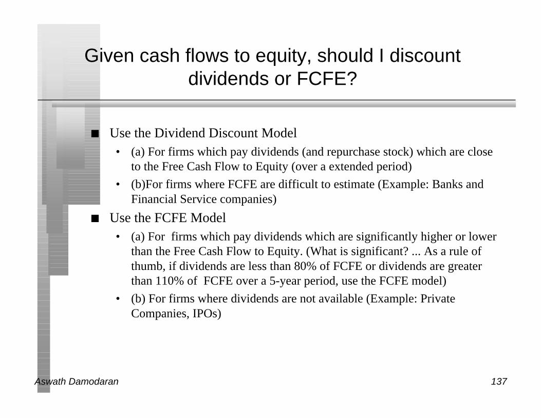
Given cash flows to equity, should I discountdividends or FCFE?
n Use the Dividend Discount Model• (a) For firms which pay dividends (and repurchase stock) which are close
to the Free Cash Flow to Equity (over a extended period)
• (b)For firms where FCFE are difficult to estimate (Example: Banks andFinancial Service companies)
n Use the FCFE Model• (a) For firms which pay dividends which are significantly higher or lower
than the Free Cash Flow to Equity. (What is significant? ... As a rule ofthumb, if dividends are less than 80% of FCFE or dividends are greaterthan 110% of FCFE over a 5-year period, use the FCFE model)
• (b) For firms where dividends are not available (Example: PrivateCompanies, IPOs)

Aswath Damodaran 138
What discount rate should I use?
n Cost of Equity versus Cost of Capital• If discounting cash flows to equity -> Cost of Equity
• If discounting cash flows to the firm -> Cost of Capital
n What currency should the discount rate (risk free rate) be in?• Match the currency in which you estimate the risk free rate to the currency
of your cash flows
n Should I use real or nominal cash flows?• If discounting real cash flows -> real cost of capital
• If nominal cash flows -> nominal cost of capital
• If inflation is low (<10%), stick with nominal cash flows since taxes arebased upon nominal income
• If inflation is high (>10%) switch to real cash flows

Aswath Damodaran 139
Which Growth Pattern Should I use?
n If your firm is• large and already growing at a rate close to or lower than the overall
growth rate of the economy, or
• constrained by regulation from growing at rate faster than the economy
• has the characteristics of a stable firm (average risk & reinvestment rates)
Use a Stable Growth Model
n If your firm• is large & growing at a moderate rate (≤ Overall growth rate + 10%) or
• has a single product & barriers to entry with a finite life (e.g. patents)
Use a 2-Stage Growth Modeln If your firm
• is small and growing at a very high rate (> Overall growth rate + 10%) or
• has significant barriers to entry into the business
• has firm characteristics that are very different from the norm
Use a 3-Stage Model

Aswath Damodaran 140
The Building Blocks of Valuation
Choose aCash Flow Dividends
Expected Dividends to
Stockholders
Cashflows to Equity
Net Income
- (1- δ) (Capital Exp. - Deprec’n)
- (1- δ) Change in Work. Capital
= Free Cash flow to Equity (FCFE)
[δ = Debt Ratio]
Cashflows to Firm
EBIT (1- tax rate)
- (Capital Exp. - Deprec’n)
- Change in Work. Capital
= Free Cash flow to Firm (FCFF)
& A Discount Rate Cost of Equity
Basis: The riskier the investment, the greater is the cost of equity.
Models:
CAPM: Riskfree Rate + Beta (Risk Premium)
APM: Riskfree Rate + Σ Betaj (Risk Premiumj): n factors
Cost of Capital
WACC = ke ( E/ (D+E))
+ kd ( D/(D+E))
kd = Current Borrowing Rate (1-t)
E,D: Mkt Val of Equity and Debt
& a growth pattern
t
g
Stable Growth
g
Two-Stage Growth
|High Growth Stable
g
Three-Stage Growth
|High Growth StableTransition
Aswath Damodaran 141
6. Tying up Loose Ends

Aswath Damodaran 142
Dealing with Cash
n The simplest and most direct way of dealing with cash and marketablesecurities is to keep it out of the valuation - the cash flows should bebefore interest income from cash and securities, and the discount rateshould not be contaminated by the inclusion of cash. (Use betas of theoperating assets alone to estimate the cost of equity).
n Once the firm has been valued, add back the value of cash andmarketable securities.• If you have a particularly incompetent management, with a history of
overpaying on acquisitions, markets may discount the value of this cash.

Aswath Damodaran 143
How much cash is too much cash?
Cash as a Percentage of Value of Firm: US Firms in December 1997
0
200
400
600
800
1000
1200
1400
1600
1800
< 2.5% 2.5 -5%
5 -7.50%
7.5 -10%
10 -15%
15 -20%
20 -25%
25 -30%
> 30%
Cash % of Value
Num
ber
of
Fir
ms

Aswath Damodaran 144
The Value of Cash
n Implicitly, we are assuming here that the market will value cash atface value. Assume now that you are buying a firm whose only asset ismarketable securities worth $ 100 million. Can you ever consider ascenario where you would not be willing to pay $ 100 million for thisfirm?
o Yes
o No
n What is or are the scenario(s)?

Aswath Damodaran 145
The Case of Closed End Funds
n Closed end funds are mutual funds, with a fixed number of shares.Unlike regular mutual funds, where the shares have to trade at netasset value (which is the value of the securities in the fund), closed endfunds shares can and often do trade at prices which are different fromthe net asset value.
n The average closed end fund has always traded at a discount on netasset value (of between 10 and 20%) in the United States.

Aswath Damodaran 146
Closed End Funds: Price and NAV
Closed End Equity Funds: December 31, 1997
0
5
10
15
20
25
30
35D
isco
unt
> 2
5%
Dis
coun
t: 2
0-2
5%
Dis
coun
t: 1
5-
20
%
Dis
coun
t: 1
0-
15
%
Dis
coun
t: 5
-10
%
Dis
coun
t: 0
-5
%
Pre
miu
m:0
-5%
Prem
ium
: 5
-10
%
Pre
miu
m:1
0-
15
%
Prem
ium
: 1
5-
20
%
Prem
ium
20
-2
5%
Prem
ium
25
-3
0%
Prem
ium
> 3
0%
Premium or Discount on NAV
Num
ber
of
Funds

Aswath Damodaran 147
A Simple Explanation for the Closed EndDiscount
n Assume that you have a closed-end fund that invests in ‘average risk”stocks. Assume also that you expect the market (average riskinvestments) to make 11.5% annually over the long term. If the closedend fund underperforms the market by 0.50%, estimate the discount onthe fund.

Aswath Damodaran 148
A Premium for Marketable Securities
n Some closed end funds trade at a premium on net asset value. Forinstance, the Thai closed end funds were trading at a premium ofroughly 40% on net asset value and the Indonesian fund at a premiumof 80%+ on NAV on December 31, 1997. Why might an investor bewilling to pay a premium over the value of the marketable securities inthe fund?

Aswath Damodaran 149
Berkshire Hathaway
Berkshire Hathaway
0
5000
10000
15000
20000
25000
30000
35000
40000
45000
19
87
19
88
19
89
19
90
19
91
19
92
19
93
19
94
19
95
19
96
19
97
Year
Val
ue P
er
Shar
e
0.00%
20.00%
40.00%
60.00%
80.00%
100.00%
120.00%
140.00%
Pre
miu
m o
ver
Book
Val
ue
Market Value/ShareBook Value/SharePremium over Book Value

Aswath Damodaran 150
Dealing with Other Non-Operating Assets
n The more difficult assets to value are minority holdings in subsidiaries.The right way to value these holdings is to value the subsidiariesthemselves, and take the firm’s ownership portion of this value.Unfortunately, accounting standards do not allow for muchtransparency, especially when the subsidiaries are not

Aswath Damodaran 151
Equity Value and Per Share Value: A Test
n Assume that you have done an equity valuation of Microsoft. The totalvalue for equity is estimated to be $ 400 billion and there are 5 billionshares outstanding. What is the value per share?

Aswath Damodaran 152
An added fact
n In 1999, Microsoft had 500 million options outstanding, granted toemployees over time. These options had an average exercise price of $20 (the current stock price is $ 80). Estimate the value per share.

Aswath Damodaran 153
Equity Value and Per Share Value
n The conventional way of getting from equity value to per share valueis to divide the equity value by the number of shares outstanding. Thisapproach assumes, however, that common stock is the only equityclaim on the firm.
n In many firms, there are other equity claims as well including:• warrants, that are publicly traded
• management and employee options, that have been granted, but do nottrade
• conversion options in convertible bonds
• contingent value rights, that are also publicly traded.
n The value of these non-stock equity claims has to be subtracted fromthe value of equity before dividing by the number of sharesoutstanding.

Aswath Damodaran 154
Option Grants at US Firms

Aswath Damodaran 155
Warrants
n A warrant is a security issued by a company that provides the holderwith the right to buy a share of stock in the company at a fixed priceduring the life of the warrant.
n A warrant is therefore a long term call option on the equity of the firmand can be valued using option pricing models.
n Warrants and other equity options issued by the firm are claims on theequity of the firm and have to be treated as equity, which has relevancefor:• estimating debt and equity for the leverage calculation
• estimating per share value from total equity value

Aswath Damodaran 156
Why firms use warrants and options
n Warrants are priced based upon the implied volatility assigned to theunderlying stock; the greater the volatility, the greater the value. To thedegree that the market overestimates the firm’s volatility, the firm maygain by using warrants and option-like securities.
n Warrants, by themselves, create no cash obligations at the time of theissue. Consequently, issuing warrants is a good way for a high growthfirm to raise funds, especially when current cash flows are low or non-existent.
n For financial officers who are sensitive to the dilution created byissuing common stock, warrants seem to provide the best of bothworlds –– they do not create any new additional shares currently,while they raise equity investment funds for current use.

Aswath Damodaran 157
Convertible Bonds
n A convertible bond is a bond that can be converted into a pre-determined number of shares, at the option of the bond holder.
n While it generally does not pay to convert at the time of the bondissue, conversion becomes a more attractive option as stock pricesincrease.
n A convertible bond can be considered to be made up of two securities -a straight bond and a conversion option.
n Firms generally add conversions options to bonds to lower the interestrate paid on the bonds.

Aswath Damodaran 158
The Straight Bond Component
n Embedded in every convertible bond is a straight bond component.
n The easiest way to value the straight bond component is to act as if theconversion option does not exist and value the bond. This can beaccomplished as follows:• Step 1: Obtain the coupon rate on the convertible bond (which will
generally be low because of the conversion option)
• Step 2: Estimate the interest rate that the company would have had to payif it had issued a straight bond. This can be obtained either from otherbonds that the company has outstanding or from its bond rating.
• Step 3: Using the maturity of the convertible bond, the coupon rate andthe market interest rate, estimate the value of the bond as:
Value of Bond = PV of coupons at market interest rate + PV of face value ofbond at market interest rate
n The straight bond component is clearly debt.

Aswath Damodaran 159
Factors in Using Option Pricing Models toValue Convertibles and Warrants
n Option pricing models can be used to value the conversion option withthree caveats –• conversion options are long term, making the assumptions about constant
variance and constant dividend yields much shakier,
• conversion options result in stock dilution, and
• conversion options are often exercised before expiration, making itdangerous to use European option pricing models.
n These problems can be partially alleviated by using a binomial optionpricing model, allowing for shifts in variance and early exercise, andfactoring in the dilution effect

Aswath Damodaran 160
Steps in Getting to Value Per Share
n Step 1: Value the firm, using discounted cash flow or other valuationmodels.
n Step 2:Subtract out the value of the outstanding debt to arrive at thevalue of equity. Alternatively, skip step 1 and estimate the of equitydirectly.
n Step 3:Subtract out the market value (or estimated market value) ofother equity claims:• Value of Warrants = Market Price per Warrant * Number of Warrants :
Alternatively estimate the value using OPM
• Value of Conversion Option = Market Value of Convertible Bonds -Value of Straight Debt Portion of Convertible Bonds
n Step 4:Divide the remaining value of equity by the number of sharesoutstanding to get value per share.

Aswath Damodaran 161
An Example: Valuing Sterling Software
n The equity in Sterling Software was valued at $2,036 million, basedupon projected cash flows
n The firm has two equity options outstanding:• The firm has 100,000 bonds outstanding, each of which can be converted
into 20 shares of stock. The market price of each convertible bond is$1,750 and the face value is $ 1000; coupon rate of 5.75%; expires in 8years; Bond Rating is A-; Interest rate on comparable debt = 7.50%;
• The firm has 1.8 million warrants outstanding, with a strike price of $ 55per share; these are trading at $ 30 per share

Aswath Damodaran 162
Estimating the Value of Options
n Convertible Debt has market value of $ 175 million; face value of $115 million; coupon rate of 5.75%; expires in 8 years;• Bond Rating is A-; Interest rate on comparable debt = 7.50%;
• Coupon on Convertible Debt = .0575 * 115 million = $ 6.6125 million
• Value of Straight Debt Portion of Convertible Debt = $ 6.6125 (PV ofAnnuity,7.5%,8 years) + $ 115 million/1.0758 = $ 103.21 million
• Value of Conversion Option in Debt = Market Value of Convertible Debt- Straight Debt Portion = $ 175 - $ 103 = $ 72 million :Equity
n Value of Warrants = Number of warrants * Warrant Price = 1.8million warrants * $ 30 = $ 54 million

Aswath Damodaran 163
Value Per Share: Sterling Software
Value of Equity = $2,036 million
- Value of Equity in Convertible Debt = $ 72 million
- Value of Equity in Warrants = $ 54 million
Value of Equity in Common Stock = $ 1,910 million
/ Number of Shares outstanding = 25.50 million
Value per Share = $ 74.90

Aswath Damodaran 164
A Comparison to Other Approaches
n The Conservative Approach: Estimate the total number of sharesoutstanding, including those in the options.
Value of Equity per share = Value of Equity/Fully diluted # of shares
= $ 2,036/ (25.50 + 2 + 1.8) = $ 69.49
n The Treasury Stock Approach: Add the expected proceeds fromexercise to the numerator before dividing by the number of sharesoutstanding:
Value of Equity per share = (Value of Equity + Proceeds from Exercise)/Fully diluted number of shares
= (2036 + 100 + 1.8*55)/(25.5 + 2 + 1.8) = $ 76.28