EQUITY DERIVATIVES€¦ · Fig. 5.14 FX smile for 1-month options on EURUSD at two different points in time 130 Fig. 5.15 Volatility against strike for 3-month options. S&P 500 equity

CORPORATE AND INSTITUTIONAL APPLICATIONS

NEIL C. SCHOFIELD

EQUIT Y DERIVATIVES

Equity Derivatives

Neil C Schofield

Equity DerivativesCorporate and Institutional Applications

ISBN 978-0-230-39106-2 ISBN 978-0-230-39107-9 (eBook)DOI 10.1057/978-0-230-39107-9

Library of Congress Control Number: 2016958283

© The Editor(s) (if applicable) and The Author(s) 2017The author(s) has/have asserted their right(s) to be identified as the author(s) of this work in accordance with the Copyright, Designs and Patents Act 1988.This work is subject to copyright. All rights are solely and exclusively licensed by the Publisher, whether the whole or part of the material is concerned, specifically the rights of translation, reprinting, reuse of illustrations, recitation, broadcasting, reproduction on microfilms or in any other physical way, and transmission or informa-tion storage and retrieval, electronic adaptation, computer software, or by similar or dissimilar methodology now known or hereafter developed.The use of general descriptive names, registered names, trademarks, service marks, etc. in this publication does not imply, even in the absence of a specific statement, that such names are exempt from the relevant protective laws and regulations and therefore free for general use.The publisher, the authors and the editors are safe to assume that the advice and information in this book are believed to be true and accurate at the date of publication. Neither the publisher nor the authors or the editors give a warranty, express or implied, with respect to the material contained herein or for any errors or omissions that may have been made. The publisher remains neutral with regard to jurisdictional claims in published maps and institutional affiliations.

Cover image © dowell / Getty

Printed on acid-free paper

This Palgrave Macmillan imprint is published by Springer NatureThe registered company is Macmillan Publishers Ltd.The registered company address is: The Campus, 4 Crinan Street, London, N1 9XW, United Kingdom

Neil C SchofieldVerwood, Dorset, United Kingdom

v

Like the vast majority of authors, I have been able to benefit from the insights of many people while writing this book.

First and foremost, I must thank my friend and fellow trainer, David Oakes of Dauphin Financial Training. On more occasions than he cares to remem-ber David has kindly answered my queries in his normal cheerful manner. If you ever have a question on finance, I can assure you that David will know the answer! I must also thank Yolanda Clatworthy who spent a significant amount of time reviewing chapter three. Her insights have added enormous value to the chapter. Stuart Urquhart arranged for me to have access to Barclays Live and the quality of the data and screenshots has added significant value to the text. Over the years that I have known Stuart he has been a great supporter of all my writing and training activities often when the benefit to himself is marginal. A true gentleman. Many thanks to Doug Christensen who gave permission for the Barclays Live data to be used.

Aaron Brask and Frans DeWeert both critiqued the original text proposal and made a number of useful pointers as to how the scope could be improved. Although I had to drop some of the suggestions due to time and space con-straints, their contributions were significant and gladly received. Also thanks to Matt Deakin of Morgan Stanley who helped clarify some equity swap set-tlement conventions. Troy Bowler was an invaluable sounding board in rela-tion to a number of topics.

Thanks also go to the many participants who have attended my classroom sessions over the years. The immediacy of the feedback that participants pro-vide is invaluable in helping me deepen my understanding of a topic.

Acknowledgements

vi Acknowledgements

Finally, a word of thanks to my family who have always been supportive of everything that I have done. A special word of thanks to Nicki who never complains even when I work late. “V”.

Although many people helped to shape the book any mistakes are entirely my responsibility. I would always be interested to hear any comments about the text and so please feel free to contact me at [email protected] or via my website www.fmarketstraining.com.

PS. Alan and Roger—once again, two slices of white toast and a cuppa for me!

vii

1 Equity Derivatives: The Fundamentals 1

2 Corporate Actions 35

3 Equity Valuation 45

4 Valuation of Equity Derivatives 73

5 Risk Management of Vanilla Equity Options 105

6 Volatility and Correlation 139

7 Barrier and Binary Options 203

8 Correlation-Dependent Exotic Options 247

9 Equity Forwards and Futures 271

10 Equity Swaps 287

11 Investor Applications of Equity Options 315

Contents

viii Contents

12 Structured Equity Products 347

13 Traded Dividends 385

14 Trading Volatility 417

15 Trading Correlation 461

Bibliography 479

Index 481

ix

Fig. 1.1 Movements of securities and collateral: non-cash securities lending trade 13

Fig. 1.2 Movements of securities and collateral: cash securities lending trade 14Fig. 1.3 Example of an equity swap 20Fig. 1.4 Profit and loss profiles for the four main option building blocks 22Fig. 1.5 Example of expiry payoffs for reverse knock in and out options 24Fig. 1.6 At expiry payoffs for digital calls and puts 25Fig. 1.7 Overview of equity market interrelationship 32Fig. 2.1 Techniques applied to equity derivative positions dependent

on the type of takeover activity 38Fig. 3.1 The asset conversion cycle 49Fig. 4.1 Structuring and hedging a single name price return swap 82Fig. 4.2 Diagrammatic representation of possible arbitrage between

the equity, money and equity swaps markets 84Fig. 4.3 Diagrammatic representation of possible arbitrage between

the securities lending market and the equity swaps market 85Fig. 4.4 ATM expiry pay off of a call option overlaid with a stylized normal

distribution of underlying prices 92Fig. 4.5 ITM call option with a strike of $50 where the underlying price has

increased to $51 93Fig. 4.6 Increase in implied volatility for ATM call option 93Fig. 4.7 The impact of time on the value of an ATM call option 95Fig. 4.8 Relationship between option premium and the underlying price

for a call option prior to expiry 97Fig. 5.1 Relationship between an option’s premium and the underlying

asset price for a long call option prior to expiry 106Fig. 5.2 Delta for a range of underlying prices far from expiry for a

long-dated, long call option position 106

List of Figures

x List of Figures

Fig. 5.3 Delta for a range of underlying prices close to expiry for a long call option position 107

Fig. 5.4 Equity call option priced under different implied volatility assumptions 109

Fig. 5.5 Positive gamma exposure for a long call position 112Fig. 5.6 Expiry profile of delta-neutral short volatility position 114Fig. 5.7 Initial and expiry payoffs for delta-neutral short position 115Fig. 5.8 Impact on profit or loss for a 5 % fall in implied volatility on the

delta- neutral short volatility position 115Fig. 5.9 Sources of profitability for a delta-neutral short volatility trade 118Fig. 5.10 Theta for a 1-year option over a range of spot prices 121Fig. 5.11 The theta profile of a 1-month option for a range of spot prices 122Fig. 5.12 Pre- and expiry payoff values for an option, which displays

positive theta for ITM values of the underlying price 123Fig. 5.13 Vega for a range of spot prices and at two different maturities 127Fig. 5.14 FX smile for 1-month options on EURUSD at two different

points in time 130Fig. 5.15 Volatility against strike for 3-month options. S&P 500 equity index 131Fig. 5.16 Implied volatility against maturity for a 100 % strike option

(i.e. ATM spot) S&P 500 equity index 132Fig. 5.17 Volatility surface for S&P 500 as of 25th March 2016 133Fig. 5.18 Volgamma profile of a long call option for different maturities

for a range of spot prices. Strike price = $15.15 135Fig. 5.19 Vega and vanna exposures for 3-month call option for a range

of spot prices. Option is struck ATM forward 136Fig. 5.20 Vanna profile of a long call and put option for different

maturities and different degrees of ‘moneyness’ 137Fig. 6.1 A stylized normal distribution 140Fig. 6.2 Upper panel: Movement of Hang Seng (left hand side) and

S&P 500 index (right hand side) from March 2013 to March 2016. Lower panel: 30-day rolling correlation coefficient over same period 145

Fig. 6.3 The term structure of single-stock and index volatility indicating the different sources of participant demand and supply 146

Fig. 6.4 Level of the S&P 500 and 3-month implied volatility for a 50 delta option. March 2006–March 2016 151

Fig. 6.5 Implied volatility for 3-month 50 delta index option versus 3-month historical index volatility (upper panel). Implied volatility minus realized volatility (lower panel). March 2006–March 2016 152

Fig. 6.6 Average single-stock implied volatility versus average single-stock realized volatility (upper panel). Implied volatility minus realized volatility (lower panel). March 2006–March 2016 153

List of Figures xi

Fig. 6.7 Implied volatility of 3-month 50 delta S&P index option versus average implied volatility of 50 largest constituent stocks. March 2006–March 2016 154

Fig. 6.8 Realized volatility of 3-month 50 delta S&P 500 index option versus average realized volatility of 50 largest constituent stocks. March 2006–March 2016 155

Fig. 6.9 Example of distribution exhibiting negative skew. The columns represent the skewed distribution while a normal distribution is shown by a dotted line 156

Fig. 6.10 Volatility skew for 3-month ATM options written on the S&P 500 equity index. The X axis is the strike of the option as a percentage of the current spot price 158

Fig. 6.11 Volatility smile for Blackberry. Implied volatility (Y axis) measured relative to the delta of a 3-month call option 159

Fig. 6.12 Volatility skew for Reliance industries 160Fig. 6.13 S&P 500 index volatility (left hand side) plotted against the skew

measured in percent (right hand side). March 2006–March 2016 163Fig. 6.14 Variance swap strike and ATM forward implied forward volatility

for S&P 500 (upper panel). Variance swap divided by ATM forward volatility for S&P 500 (lower panel). March 2011– March 2016 165

Fig. 6.15 Evolution of the volatility skew over time. Skewness measured as the difference between the implied volatilities of an option struck at 90 % of the market less that of an option struck at 110 %. The higher the value of the number the more the market is skewed to the downside (i.e. skewed towards lower strike options) 166

Fig. 6.16 Implied volatility of 3-month ATM S&P 500 option plotted against the 3-month volatility skew 167

Fig. 6.17 Term structure of volatility for an S&P 500 option struck at 80 % of spot 169



Fig. 6.20 Slope of term structure of S&P 500 implied volatility. Term structure is measured as 12-month implied volatility minus 3-month volatility. An increase in the value of the Y axis indicates a steepening of the slope 173

Fig. 6.21 Implied volatility of 3-month 50 delta S&P 500 index option (Left hand axis) versus the slope of the index term structure (right hand axis). March 2006–March 2016 174

Fig. 6.22 Volatility skew for S&P options with different maturities. Data based on values shown in Table 6.1 175

xii List of Figures

Fig. 6.23 Time series of 3-month index implied volatility plotted against 36-month index implied volatility. March 2006–March 2016 176

Fig. 6.24 Chart shows the change in 3-month ATM spot implied volatility vs. change in 36-month ATM spot volatility for the S&P 500 index. March 2006–March 2016 178

Fig. 6.25 A ‘line of best fit’ for a scattergraph of changes in 36-month implied volatility (Y axis) against changes in 3-month implied volatility (x axis). S&P 500 index, March 2006–March 2016 179

Fig. 6.26 Implied volatility of 3-month 50 delta S&P 500 index against 3-month implied correlation. March 2006–March 2016 183

Fig. 6.27 Level of S&P 500 cash index against 3-month index implied correlation. March 2006–March 2016 184

Fig. 6.28 One-month implied correlation of Hang Seng Index. March 2006–March 2016 186

Fig. 6.29 Three-month Implied correlation minus realized correlation. S&P 500 equity index 187

Fig. 6.30 Term structure of S&P 500 implied correlation. Twelve-month minus 3-month implied correlation. March 2006–March 2016 188

Fig. 6.31 Implied volatility of 3-month 50 delta S&P 500 index option (left hand axis) plotted against slope of correlation term structure (right hand axis). The correlation term structure is calculated as 12-month minus 3-month implied correlation. A negative value indicates an inverted term structure 189

Fig. 6.32 Implied volatility of S&P 500 index options from 1996 to 2016 191Fig. 6.33 Realized volatility of S&P 500 from 1996 to 2016 192Fig. 6.34 Three-month implied and realized volatility for S&P 500 194Fig. 6.35 Volatility cone for S&P 500 index options. Data as of

28th July 2014 195Fig. 6.36 S&P 500 index implied correlation. March 1996–March 2016 197Fig. 6.37 S&P 500 index realized correlation. March 1996–March 2016 198Fig. 6.38 Correlation cone for S&P 500. Data as of 28 July 2014 199Fig. 7.1 Taxonomy of barrier options 204Fig. 7.2 Value of ‘down and in’ call option prior to maturity.

Initial spot 100, strike 100, barrier 90 209Fig. 7.3 Delta of the down and in call option. Initial spot 100,

strike 100, barrier 90 210Fig. 7.4 The gamma for a down and in call option. Initial spot 100,

strike 100, barrier 90 211Fig. 7.5 Theta profile for down and in call. Initial spot 100, strike 100,

barrier 90 212Fig. 7.6 Vega profile for down and in call option. Initial spot 100,

strike 100, barrier 90 212

List of Figures xiii

Fig. 7.7 Payoff profile of down and out call option. Initial spot 100, strike 100, barrier 90 213

Fig. 7.8 Delta of a down and out call option with a barrier of 90 and a strike of 100 213

Fig. 7.9 Gamma of a down and out call option with a barrier of 90 and a strike of 100 214

Fig. 7.10 Theta of a down and out call option with a barrier of 90 and a strike of 100 214

Fig. 7.11 Vega of a down and out call option with a barrier of 90 and a strike of 100 215

Fig. 7.12 Up and in call option. Premium vs. underlying price; strike price 100, barrier 110 216

Fig. 7.13 Delta profile of an up and in call option. Strike price 100, barrier 110 216

Fig. 7.14 Gamma profile of an up and in call option Strike price 100, barrier 110 217

Fig. 7.15 The theta value of an up and in call option. Strike price 100, barrier 110 218

Fig. 7.16 The vega value of an up and in call option. Strike price 100, barrier 110 218

Fig. 7.17 Payoff diagram of spot price vs. premium for up and out call option 219

Fig. 7.18 The delta profile for an up and out call option. Strike price 100, barrier 110 219

Fig. 7.19 Gamma exposure of the up and out call option. Strike price 100, barrier 110 220

Fig. 7.20 Theta profile for long up and out call option. Strike price 100, barrier 110 220

Fig. 7.21 Vega profile of up and out call option. Strike price 100, barrier 110 221

Fig. 7.22 Payoff profiles for up and out call option close to and at expiry. Strike 100, barrier 110 222

Fig. 7.23 The delta of an up and out call option close to expiry. Strike 100, barrier 110 222

Fig. 7.24 The pre- and post-expiry values of a down and in put option (upper diagram) with associated delta profile (lower diagram) 224

Fig. 7.25 Expiry and pre-expiry payoffs for a knock in call (‘down and in’). Strike price 90, barrier 95 227

Fig. 7.26 Delta of down and in reverse barrier call option. Strike price 90, barrier 95 228

Fig. 7.27 Gamma of down and in reverse barrier call option. Strike price 90, barrier 95 228

xiv List of Figures

Fig. 7.28 Theta of down and in reverse barrier call option. Strike price 90, barrier 95 229

Fig. 7.29 Vega of down and in reverse barrier call option. Strike price 90, barrier 95 230

Fig. 7.30 Down and out call option. Strike price 90, barrier 95 230Fig. 7.31 The delta of a down and out call option. Strike price 90,

barrier 95 231Fig. 7.32 The gamma of a down and out call option. Strike price 90,

barrier 95 232Fig. 7.33 The theta of a long down and out call option. Strike price 90,

barrier 95 232Fig. 7.34 The vega of a down and out call option. Strike price 90, barrier 95 233Fig. 7.35 Pre-expiry and expiry payoff values of a ‘one touch’ option 238Fig. 7.36 Delta of one touch binary option 239Fig. 7.37 Gamma value of a one touch option 239Fig. 7.38 Theta profile of a one touch option 240Fig. 7.39 The vega exposure of a one touch option 240Fig. 7.40 Pre- and expiry payoffs for a European-style binary option 241Fig. 7.41 The delta profile of a European binary call option against the

underlying price and maturity 242Fig. 7.42 The gamma profile of a European binary call option against the

underlying price and maturity 243Fig. 7.43 The theta profile of a European binary call option against the

underlying price and maturity 244Fig. 7.44 The vega profile of a European binary call option against the

underlying price and maturity 245Fig. 7.45 The vega profile of a European binary option shortly before expiry 245Fig. 8.1 Thirty-day rolling correlation (right hand axis) between Chevron

and ExxonMobil 249Fig. 9.1 Relationship between spot and forward prices 272Fig. 10.1 Using total return equity swaps to exploit expected movements

in the term structure of equity repo rates 297Fig. 10.2 Closing out a 6-year total return swap, 1 year after inception

with a 5-year total return swap 298Fig. 10.3 Setting up an equity swap with a currency component 300Fig. 10.4 Cash and asset flows at the maturity of the swap 301Fig. 10.5 Total return equity swap used for acquiring a target company 303Fig. 10.6 Prepaid forward plus equity swap 306Fig. 10.7 Synthetic sale of shares using a total return swap 307Fig. 10.8 Relative performance swap 308Fig. 11.1 Net position resulting from a long cash equity portfolio and

a long ATM put option 317

List of Figures xv

Fig. 11.2 Profit and loss profile for a long equity position overlaid with an OTM put 318

Fig. 11.3 Long position in an index future combined with the purchase of an ATM put and the sale of an OTM put 319

Fig. 11.4 Expiry payoff from a zero premium collar 320Fig. 11.5 Zero premium collar constructed using ‘down and out’ options 321Fig. 11.6 At expiry payoff of a call spread. Position is based on a notional

of 100,000 shares 329Fig. 11.7 At expiry payoff of a 1 × 2 call spread. Position is based on a

notional of 100,000 shares for the long call position and 200,000 shares for the short call position 331

Fig. 11.8 At expiry delta-neutral long straddle position. Position is based on a notional of 100,000 shares per leg 334

Fig. 11.9 Long strangle. Position is based on a notional of 100,000 shares per leg 336

Fig. 11.10 At expiry payoff of delta-neutral short straddle. Sell a call and a put with the strikes set such that the net delta is zero. Based on a notional amount of 100,000 shares per leg 336

Fig. 11.11 At expiry payoff of 25 delta short strangle. The strike of each option is set at a level that corresponds to a delta value of 25. Based on an option notional of 100,000 shares per leg 337

Fig. 11.12 Covered call. Investor is long the share and short an OTM call option. Example is based on a notional position of 100,000 shares 338

Fig. 11.13 Call spread overwriting. Example is based on a notional position of 100,000 shares 339

Fig. 11.14 Evolution of volatility skew for BBRY. Hashed line shows the initial volatility values; unbroken line shows final values 345

Fig. 12.1 Payoff from a ‘twin win’ structured note. Solid line shows the payoff if the barrier is not breached. Dotted line shows the payoff if the barrier is breached; this payoff is shown as being slightly offset for ease of illustration 365

Fig. 12.2 Replicating a binary call option with a call spread 370Fig. 12.3 Binary option hedged with call spread 370Fig. 12.4 Payoff and risk management profiles for ‘down and in’

put option. Upper panel shows at and pre-expiry payoff; middle panel is the vega profile while lowest panel is the delta profile 372

Fig. 12.5 Level of EURO STOXX 50 (SX5E) vs. 2-year implied volatility. September 2014–September 2015 375

Fig. 12.6 Vega profile of a risk reversal. In this example the risk reversal comprises of the sale of a short put struck at 90 and the purchase of a long call at 110. Vega is measured on the Y axis in terms of ticks, that is, the minimum price movement of the underlying asset 377

xvi List of Figures

Fig. 12.7 Time series for 2-year volatility skew for EURO STOXX 50. September 2010–September 2015. Skew measured as the volatility of an option struck at 90 % of spot minus the volatility of an option struck at 110 % of spot 378

Fig. 12.8 Term structure of EURO STOXX 50. July 13th 2015 379Fig. 13.1 Cash flows on a generic dividend swap 392Fig. 13.2 Evolution of EURO STOXX dividend futures; 2014 and 2015

maturities. Data covers period July 2014–July 2015 400Fig. 13.3 Implied volatility skew for options written on the December

2018 SX5E dividend future at three different points in time. X axis is the strike price as a percentage of the underlying price 402

Fig. 13.4 Term structure of implied volatility for options on SX5E dividend futures at three different points in time 403

Fig. 13.5 The relative value (RV) triangle 405Fig. 13.6 Scatter graph of slope of 2020–2018 dividend futures slope

(y axis) versus 2016 dividend future (x axis). The slope is defined as the long-dated dividend future minus the shorter-dated future. The most recent observation is highlighted with an ‘X’ 406

Fig. 13.7 Term structure of Eurex dividend futures at two different points in time 408

Fig. 13.8 Slope of term dividend future term structure (2020–2018; dotted line) versus the level of the market (2016 dividend future). Slope of term structure is the 2020 dividend future less the 2018 dividend future and is read off the left hand scale which is inverted 409

Fig. 14.1 Example of a risk reversal—equity market skew steepens 420Fig. 14.2 Change in curvature of a volatility skew. Volatilities for calls

and puts are assumed to be of equal delta value (e.g. 25 delta) 421Fig. 14.3 Pre- and at expiry payoffs for a butterfly spread trade 423Fig. 14.4 Profit and loss on a 1-year calendar spread trade after 6 months 424Fig. 14.5 Structure of a variance swap 433Fig. 14.6 Three-month realized volatility for Morgan Stanley. March 2006

to March 2016 435Fig. 14.7 Upper panel: 3-month ATM forward option implied volatility

vs. 3-month variance swap prices. Lower panel: Variance swaps minus option implied volatility. Underlying asset is S&P 500. March 2006 to March 2016 437

Fig. 14.8 Three-month variance vs. volatility for 30 delta put (70 delta call used as an approximation). Underlying index is S&P 500. March 2015 – March 2016 439

List of Figures xvii

Fig. 14.9 Upper panel: 3-month variance swap quotes for the S&P 500 (in implied volatility terms) vs. realized volatility. Lower panel: Variance swap prices minus realized volatility. March 2006 to March 2016 445

Fig. 14.10 Time series of S&P 500 variance swap strikes: 1-month, 6-months and 12 months. March 2015 to March 2016 447

Fig. 14.11 Term structure of S&P 500 variance swap quotes 448Fig. 14.12 Upper panel: 3-month variance swap quotes for EURO

STOXX 50 vs. S&P 500. Lower panel: Bottom line shows the difference between the two values. March 2013 to March 2016 449

Fig. 14.13 Three-month ATMF S&P 500 implied volatility (left hand side) against 3-month ATM implied volatility for options on CDX index (right hand side). March 2013 to March 2016 450

Fig. 15.1 Volatility flows for the equity derivatives market 462Fig. 15.2 Structure of correlation swap 465

xix

Table 1.1 Hypothetical constituents of an equity index 4Table 1.2 Illustration of impact of rights issue depending on whether

the rights are taken up or not 10Table 3.1 2015 Balance sheet for Apple Inc 48Table 3.2 2015 Income statement for Apple Inc 52Table 3.3 Abbreviated 2015 statement of cash flows for Apple Inc 53Table 4.1 Market rates used for swap valuation example 86Table 4.2 Valuation of equity swap on trade date 87Table 4.3 Impact on the value of a call and a put from a change in

the spot price 96Table 4.4 Impact on the value of a call and put from the passage of time 97Table 4.5 Impact on the value of a call and a put from a change in

implied volatility 98Table 4.6 Impact on the value of an ITM and OTM call from a change in

implied volatility (premiums shown to just two decimal places) 98Table 4.7 Impact on the value of a call and a put from a change in

the funding rate 99Table 4.8 Impact on the value of a call and a put from a change

in dividend yields 100Table 4.9 Cost of American option vs. cost of European option in

different cost of carry scenarios 101Table 5.1 Premiums and deltas for an ITM call and OTM option put

under different implied volatility conditions. Underlying price assumed to be $15.00. All other market factors are held constant 110

Table 5.2 Stylized quotation for option position 113Table 5.3 Valuation of a deeply ITM call option on a dividend-paying stock 122

List of Tables

xx List of Tables

Table 5.4 The value of an ITM long call option on a dividend-paying stock with respect to time 124

Table 5.5 The value of an ITM long put option with respect to time 125Table 5.6 Rho for long call 126Table 5.7 Psi for long call 126Table 5.8 Volatility matrix for S&P 500 as of 25th March 2016 134Table 5.9 Vanna exposures by strike and position 137Table 6.1 Volatility surface for S&P 500. Data as of 26th July 2014.

Strikes are shown as a percentage of the spot price 156Table 6.2 Premium on a 90–110 % collar under different

volatility assumptions 168Table 6.3 Implied volatilities for different market levels and strikes

over a 3-day period 180Table 6.4 Associated delta hedging activities when trading volatility

using the four option basic ‘building blocks’ 182Table 6.5 Calculating variance and standard deviation 200Table 6.6 Calculating covariance and correlation 201Table 7.1 Parameters of regular knock in and out call options 207Table 7.2 How the position of the option barrier relative to the

spot price impacts the value of knock in and knock out call options. Spot price assumed to be 100 207

Table 7.3 How the passage of time impacts the value of a knock in and knock out call option 208

Table 7.4 The impact of different levels of implied volatility on barrier and vanilla options 209

Table 7.5 Parameters of reverse barrier call options 215Table 7.6 Examples of ‘adverse’ exit risk for four barrier options

where the position is close to expiry and spot is trading near the barrier 225

Table 7.7 Parameters of two reverse barrier call options 227Table 7.8 Barrier parity for option Greeks 235Table 7.9 Taxonomy of American-style binary options 236Table 8.1 Initial market parameters for Chevron and ExxonMobil 248Table 8.2 Calculation of composite volatility for a given level of

implied volatilities 251Table 8.3 Relationship between correlation and premium for a

basket option 252Table 8.4 Four price scenarios for the two underlying shares.

Scenarios are both prices rising (#1); both prices falling (#2); price of ExxonMobil rises while price of Chevron falls (#3) and the price of ExxonMobil falls while price of Chevron rises (#4) 254

List of Tables xxi

Table 8.5 Option payoffs from ‘best of ’ and ‘worst of ’ option structures. The four scenarios in the first column reference Table 8.4 255

Table 8.6 The relationship between correlation and the value of a ‘best of ’ call option 257

Table 8.7 The relationship between correlation and the value of a ‘worst of ’ call option 258

Table 8.8 Payout of outperformance option of ExxonMobil vs. Chevron 259Table 8.9 Impact of correlation on composite volatility of an

outperformance option 262Table 8.10 Sensitivity of an outperformance option premium to a

change in correlation 262Table 8.11 Impact of relative volatilities on the premium of an

outperformance option 263Table 8.12 The payoff to a USD investor in USD of a 1-year

GBP call option 264Table 8.13 The payoff to a USD investor in USD of a 1-year quanto

call option referencing a GBP denominated share 265Table 8.14 The impact of correlation on the USD price of a

quanto option 265Table 8.15 Intuition behind negative correlation exposure of quanto

option. Scenario #1 is a rising share price and a rising exchange rate (GBP appreciation); scenario #2 is a falling share price and falling exchange rate; scenario #3 is a falling share price and rising exchange rate while scenario #4 is a rising share price and falling exchange rate 266

Table 8.16 The payoff to a USD investor in USD of a 1-year composite call option referencing a GBP denominated share 267

Table 8.17 The impact of correlation on the USD price of a composite option 268

Table 8.18 Intuition behind negative correlation exposure of composite option 268

Table 8.19 Expiry payoffs from vanilla, composite and quanto options. Quanto and composite options are priced with zero correlation and FX volatility assumed to be 8 % 269

Table 8.20 Summary of correlation-dependent options covered in the chapter and their respective correlation exposures 270

Table 9.1 The impact of a change in the market factors that influence forward prices, all other things assumed unchanged 273

Table 9.2 Composition of equity portfolio to be hedged 276Table 9.3 Initial values for FTSE 100 and S&P 500 spot indices and

index futures 280Table 9.4 Values for indices and futures after 1 month 280

xxii List of Tables

Table 9.5 Term structure of index futures prices 281Table 10.1 Cash flows to investor and bank from sale of shares

combined with equity swap 294Table 10.2 Summary of equity repo exposures for a variety of

derivative positions 296Table 11.1 Cash flows at maturity for a prepaid variable

forward transaction 324Table 11.2 Return on investment for a variety of option strikes

and final share prices 328Table 11.3 Comparison of directional strategies 331Table 11.4 Market data for BBRY and APPL 341Table 12.1 Potential ‘at maturity’ payoffs from a capital protected

structured note 349Table 12.2 Payoff from structured note assuming 90 % capital protection

and two barrier options 352 Table 12.3 Factors that impact the participation rate of a capital

protected note 354Table 12.4 At maturity returns for reverse convertible investor 356Table 12.5 Return on a ‘vanilla’ reverse convertible vs. reverse

convertible with a knock in put 358Table 12.6 Comparison of the returns on a vanilla reverse convertible

with a deposit and a holding in the physical share. The return on the cash shareholding is calculated as the change in the share price to which the dividend yield is added 358

Table 12.7 Expiry payout from Twin Win structured note 364Table 12.8 Potential investor returns on hybrid security 365Table 13.1 Eurex EURO STOXX 50 Index futures contract specification 387Table 13.2 EURO STOXX 50 Index dividend futures. Quotation is

dividend index points equivalent 390Table 13.3 Barclays Bank dividend futures. Quotation is on a dividend

per share basis 390Table 13.4 Index dividend price quotes 392Table 13.5 Contract specification for dividend options on SX5E 401Table 14.1 Quoting conventions for a butterfly spread from a market

maker’s perspective 423Table 14.2 Expiry payout from a ‘double digital no touch option’ 426Table 14.3 Determining which options will be included in the VIX®

calculation 427Table 14.4 Contract specification for the VIX future 428Table 14.5 Contract specification for options on VIX® futures 430Table 14.6 Payoff on a long variance swap position vs. long volatility

swap position. Both positions assumed to have a vega notional $100,000 and strike of 16 % 434

List of Tables xxiii

Table 14.7 Calculation of realized volatility 444Table 14.8 Calculation of realized variance for vanilla variance swap 455Table 14.9 Calculation of realized volatility for conditional and

corridor variance swaps. Squared returns are only included if the index trades above 6300 on the previous day 456

Table 15.1 Initial market parameters for Chevron and ExxonMobil 466Table 15.2 Components of a dispersion trade 472Table 15.3 Term sheet for hypothetical dispersion trade 474Table 15.4 Structuring a variance swap dispersion trade on the

EURO STOXX 50 474Table 15.5 Calculation of dispersion option payoff 476Table 15.6 Calculation of option payoff in a ‘high’ dispersion scenario 477

1© The Author(s) 2017N. Schofield, Equity Derivatives, DOI 10.1057/978-0-230-39107-9_1

1Equity Derivatives: The Fundamentals

1.1 Chapter Overview

The objective of this chapter is to provide the reader with an overview of the main concepts and terminology of the ‘cash’ equity market that is directly relevant to the equity derivatives market.1 Although the products covered in this chapter will reappear throughout the text, certain variants (e.g. dividend and variance swaps) will be described in the chapters where they feature most prominently. The products and concepts covered in this chapter are as follows:

• ‘Cash’ equity markets• Equity derivative products• Market participants

1.2 Fundamental Concepts

1.2.1 Corporate Capital Structures

In general terms there are three ways in which a company can borrow money:

• Bank loans• Bond issuance• Equity issuance

1 For readers looking for more detail one suggested reference is Chisholm, A (2009) ‘An introduction to capital markets’ John Wiley and Sons.

These borrowings are shown on a company’s financial statements as lia-bilities since they represent monies owed to other entities and can be used to finance the purchase of assets, that is, items owned by the company. Collectively, these three sources of funds are loosely referred to as ‘capital’ and taken collectively represent a company’s capital structure. In an ideal world the assets purchased by these liabilities should generate sufficient income to finance the return to the different providers of capital. The interest on bank loans and bonds will be contractual interest, typically variable for bank loans and fixed for the issued bonds. Equities will pay a discretionary dividend whose magnitude should reflect the fact that in the event of the company going out of business, shareholders will be the last to be repaid.

1.2.2 Types of Equity

As in many aspects of finance it is common to use many different terms to describe the same concept. For example, equities can also be referred to inter-changeably as either ‘shares’ or ‘stock’.

There are several different types of equity:

• Ordinary shares—holders of these shares have the right to vote on certain company-related issues at the annual general meeting (AGM) and will also receive any dividends announced by the company. There is something of an urban myth which suggests that shareholders ‘own’ the company, whereas in reality this is not the case.2

• Preferred shares—this class of equity sits above ordinary shares for bank-ruptcy purposes and holders will typically receive a fixed dividend payment before any ordinary shareholders are repaid.

• Cumulative preference shares—these are a version of preferred shares where if the company does not have sufficient cash flow to pay the dividend in any given year it must be paid in the following year or whenever the com-pany has generated sufficient profits. Any dividend arrears must be paid off before dividends can be paid to the ordinary shareholders.

• Treasury stock—this is not really a type of share but Treasury stock repre-sents a situation where a company has decided to repurchase some of its own shares in the market. The shares are not cancelled but are held on the balance sheet. A company may decide to repurchase its own shares if they felt they were undervalued.

2 See for example: ‘Is it meaningful to talk about the ownership of companies’ on www.johnkay.com

2 Equity Derivatives

http://www.johnkay.com

1.2.3 Equity Indices

IntroductionAn equity index is a numerical representation of the way an equity market has performed relative to some base reference date. The index is assigned an arbi-trary initial value of, say, 100 or 1000. For example, the UK FTSE 100 share index was launched on 3rd January 1984 with a base value of 1000.

They are also widely used as a benchmark for fund management perfor-mance; a fund that has generated a 5 % return would need to have its per-formance judged within some context. If ‘the market’, as defined by some agreed index, has returned 7 %, then at a very simple level the fund has underperformed.

Each of the indices will be compiled according to a different set of rules that would govern such aspects as follows:

• What constitutes an eligible security for inclusion in the index?• How often are the constituent members reviewed?• What criteria will lead to a share being removed from or added to the index?• How are new issues, mergers and restructurings reflected within the index?

Reference is sometimes made to ‘investable indices’, which refers to those indices where it is possible for market participants to purchase the constituent shares in the same proportions as the index without concerns over liquidity or without incurring significant transaction costs.

Index ConstructionGenerally speaking, there are two ways in which an index can be constructed. The simplest form of index construction uses the concept of price weighting. The value of the index is basically the sum of all the security prices divided by the total number of constituents. All the shares are equally weighted with no account taken of the relative size of the company. This type of method is rarely used but it does form the basis of how the Dow Jones Industrial Average is constructed.

The most commonly used method is market-value weighting which is based on the market capitalization of each share. This technique weights each of the con-stituent shares by the number of shares in issue so the relative size of the company will determine the impact on the index of a change in the share price. The market capitalization of a company is calculated based on the company’s ‘free float’. This is the number of shares that are freely available to purchase. So if a company were to issue new shares but wished to retain ownership of a certain proportion, only those available to the public would be included within the index calculation.


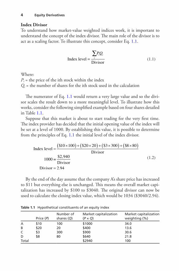
Index DivisorTo understand how market-value weighted indices work, it is important to understand the concept of the index divisor. The main role of the divisor is to act as a scaling factor. To illustrate this concept, consider Eq. 1.1.

Index level

Divisor=∑i

i iPQ

(1.1)

Where:Pi = the price of the ith stock within the indexQi = the number of shares for the ith stock used in the calculation

The numerator of Eq. 1.1 would return a very large value and so the divi-sor scales the result down to a more meaningful level. To illustrate how this works, consider the following simplified example based on four shares detailed in Table 1.1.

Suppose that this market is about to start trading for the very first time. The index provider has decided that the initial opening value of the index will be set at a level of 1000. By establishing this value, it is possible to determine from the principles of Eq. 1.1 the initial level of the index divisor.

Index level$ $ $ $

Divisor=

×( ) + ×( ) + ×( ) + ×( )10 100 20 20 3 300 8 80

1000 ==

=

$

DivisorDivisor

2 940

2 94

,

.

(1.2)

By the end of the day assume that the company A’s share price has increased to $11 but everything else is unchanged. This means the overall market capi-talization has increased by $100 to $3040. The original divisor can now be used to calculate the closing index value, which would be 1034 ($3040/2.94).

Table 1.1 Hypothetical constituents of an equity index

Price (P)Number of shares (Q)

Market capitalization (P × Q)

Market capitalization weighting (%)

A $10 100 $1000 34.0B $20 20 $400 13.6C $3 300 $900 30.6D $8 80 $640 21.8Total $2940 100


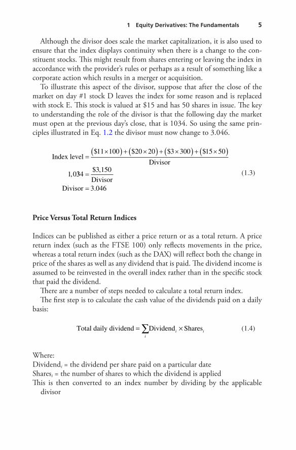
Although the divisor does scale the market capitalization, it is also used to ensure that the index displays continuity when there is a change to the con-stituent stocks. This might result from shares entering or leaving the index in accordance with the provider’s rules or perhaps as a result of something like a corporate action which results in a merger or acquisition.

To illustrate this aspect of the divisor, suppose that after the close of the market on day #1 stock D leaves the index for some reason and is replaced with stock E. This stock is valued at $15 and has 50 shares in issue. The key to understanding the role of the divisor is that the following day the market must open at the previous day’s close, that is 1034. So using the same prin-ciples illustrated in Eq. 1.2 the divisor must now change to 3.046.

Index level$ $ $ $

Divisor=

×( ) + ×( ) + ×( ) + ×( )11 100 20 20 3 300 15 50

1 0, 3343 150

3 046

=

=

$

DivisorDivisor

,

.

(1.3)

Price Versus Total Return Indices

Indices can be published as either a price return or as a total return. A price return index (such as the FTSE 100) only reflects movements in the price, whereas a total return index (such as the DAX) will reflect both the change in price of the shares as well as any dividend that is paid. The dividend income is assumed to be reinvested in the overall index rather than in the specific stock that paid the dividend.

There are a number of steps needed to calculate a total return index.The first step is to calculate the cash value of the dividends paid on a daily

basis:

Total daily dividend Dividend Shares= ×∑

ii i

(1.4)

Where:Dividendi = the dividend per share paid on a particular dateSharesi = the number of shares to which the dividend is appliedThis is then converted to an index number by dividing by the applicable

divisor


Dividend in index points

Total daily dividend

Divisor=

(1.5)

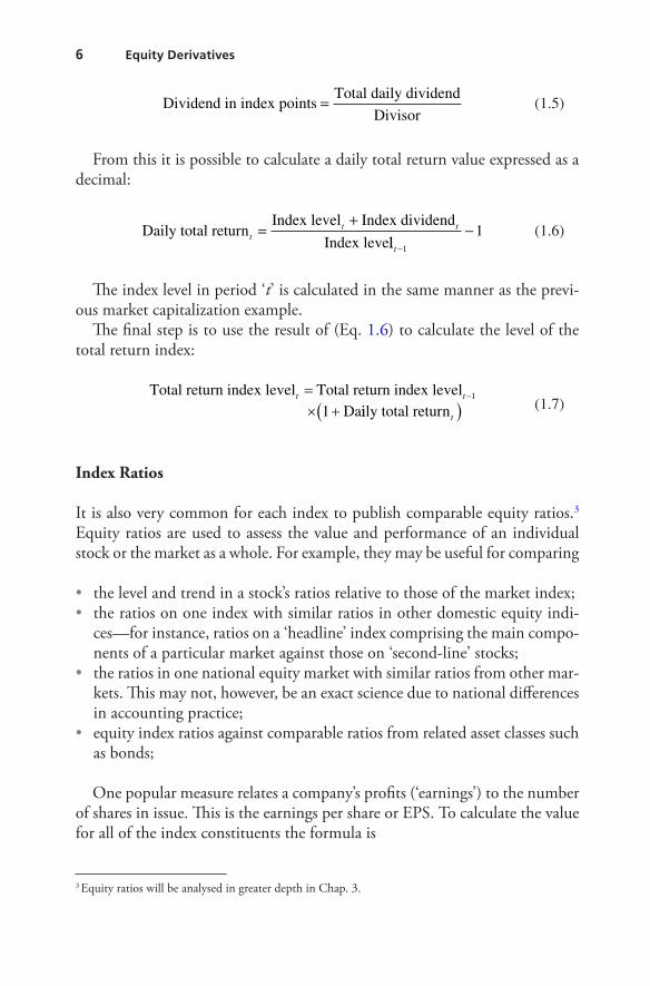
From this it is possible to calculate a daily total return value expressed as a decimal:

Daily total return

Index level Index dividend

Index levett t=+

llt−−

1

1

(1.6)

The index level in period ‘t’ is calculated in the same manner as the previ-ous market capitalization example.

The final step is to use the result of (Eq. 1.6) to calculate the level of the total return index:

Total return index level Total return index levelDa

t t=× +

−1

1 iily total returnt( ) (1.7)

Index Ratios

It is also very common for each index to publish comparable equity ratios.3 Equity ratios are used to assess the value and performance of an individual stock or the market as a whole. For example, they may be useful for comparing

• the level and trend in a stock’s ratios relative to those of the market index;• the ratios on one index with similar ratios in other domestic equity indi-

ces—for instance, ratios on a ‘headline’ index comprising the main compo-nents of a particular market against those on ‘second-line’ stocks;

• the ratios in one national equity market with similar ratios from other mar-kets. This may not, however, be an exact science due to national differences in accounting practice;

• equity index ratios against comparable ratios from related asset classes such as bonds;

One popular measure relates a company’s profits (‘earnings’) to the number of shares in issue. This is the earnings per share or EPS. To calculate the value for all of the index constituents the formula is

3 Equity ratios will be analysed in greater depth in Chap. 3.


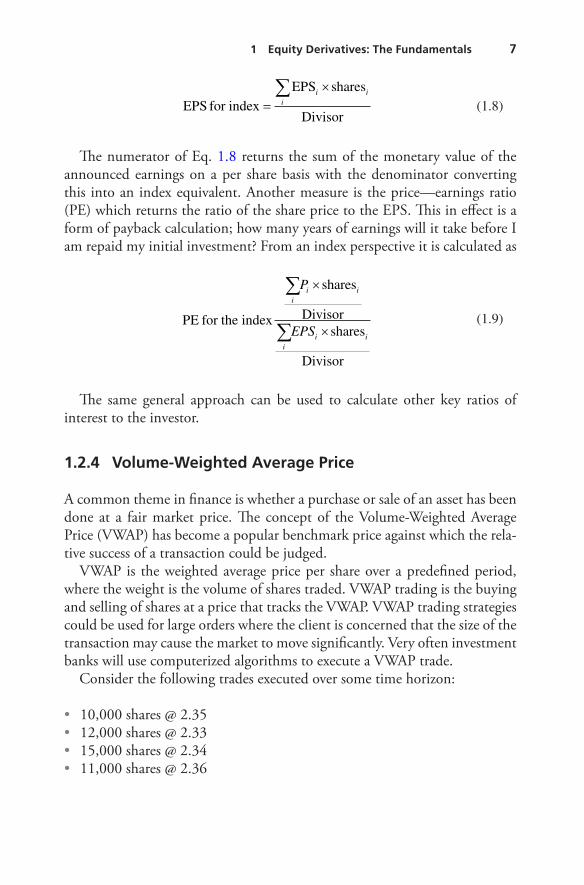
EPS for

EPSindex

shares

Divisor=

×∑i

i i

(1.8)

The numerator of Eq. 1.8 returns the sum of the monetary value of the announced earnings on a per share basis with the denominator converting this into an index equivalent. Another measure is the price—earnings ratio (PE) which returns the ratio of the share price to the EPS. This in effect is a form of payback calculation; how many years of earnings will it take before I am repaid my initial investment? From an index perspective it is calculated as

PE for the index

shares

Divisorshares

Divisor

ii i

ii i

P

EPS

∑

∑

×

×

(1.9)

The same general approach can be used to calculate other key ratios of interest to the investor.

1.2.4 Volume-Weighted Average Price

A common theme in finance is whether a purchase or sale of an asset has been done at a fair market price. The concept of the Volume-Weighted Average Price (VWAP) has become a popular benchmark price against which the rela-tive success of a transaction could be judged.

VWAP is the weighted average price per share over a predefined period, where the weight is the volume of shares traded. VWAP trading is the buying and selling of shares at a price that tracks the VWAP. VWAP trading strategies could be used for large orders where the client is concerned that the size of the transaction may cause the market to move significantly. Very often investment banks will use computerized algorithms to execute a VWAP trade.

Consider the following trades executed over some time horizon:

• 10,000 shares @ 2.35• 12,000 shares @ 2.33• 15,000 shares @ 2.34• 11,000 shares @ 2.36


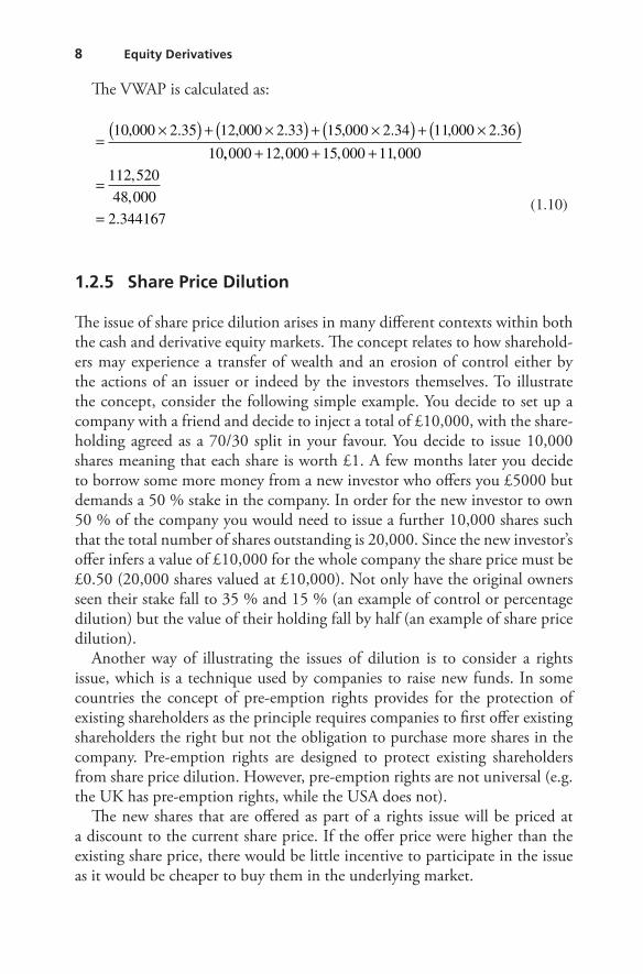
The VWAP is calculated as:

=×( ) + ×( ) + ×( ) + ×( )10 000 2 35 12 000 2 33 15 000 2 34 11000 2 36

10

, , , ,. . . .

,, , , ,

,

,

.

000 12 000 15 000 11 000

112 520

48 000

2 344167

+ + +

=

=

(1.10)

1.2.5 Share Price Dilution

The issue of share price dilution arises in many different contexts within both the cash and derivative equity markets. The concept relates to how sharehold-ers may experience a transfer of wealth and an erosion of control either by the actions of an issuer or indeed by the investors themselves. To illustrate the concept, consider the following simple example. You decide to set up a company with a friend and decide to inject a total of £10,000, with the share-holding agreed as a 70/30 split in your favour. You decide to issue 10,000 shares meaning that each share is worth £1. A few months later you decide to borrow some more money from a new investor who offers you £5000 but demands a 50 % stake in the company. In order for the new investor to own 50 % of the company you would need to issue a further 10,000 shares such that the total number of shares outstanding is 20,000. Since the new investor’s offer infers a value of £10,000 for the whole company the share price must be £0.50 (20,000 shares valued at £10,000). Not only have the original owners seen their stake fall to 35 % and 15 % (an example of control or percentage dilution) but the value of their holding fall by half (an example of share price dilution).

Another way of illustrating the issues of dilution is to consider a rights issue, which is a technique used by companies to raise new funds. In some countries the concept of pre-emption rights provides for the protection of existing shareholders as the principle requires companies to first offer existing shareholders the right but not the obligation to purchase more shares in the company. Pre-emption rights are designed to protect existing shareholders from share price dilution. However, pre-emption rights are not universal (e.g. the UK has pre-emption rights, while the USA does not).

The new shares that are offered as part of a rights issue will be priced at a discount to the current share price. If the offer price were higher than the existing share price, there would be little incentive to participate in the issue as it would be cheaper to buy them in the underlying market.


Documents

EQUITY DERIVATIVES€¦ · Fig. 5.14 FX smile for 1-month options on EURUSD at two different points in time 130 Fig. 5.15 Volatility against strike for 3-month options. S&P 500 equity