Equitable Urban Revitalization and Access to Amenities*

Nicholas B. Irwin†

Preliminary, please do not cite without author’s permission.

Version 2.1

July 18, 2016

Abstract:

Stemming urban decline and exodus from the city is a pertinent issue facing policymakers. The

success of any effort to address these issues depends on the equitability of the process, which is

especially important in lower-income minority neighborhoods disproportionately affected by

issues of environmental degradation. Using a unique set housing activity data coupled with

neighborhood level data on demographics and the environment, we examine the effect of a

targeted urban revitalization effort in Baltimore, Maryland via a quasi-experimental design. We

find neighborhoods funded by the program have higher housing sales than short-listed unfunded

neighborhoods, with increases in house renovations seen in neighborhoods with multiple funded

projects. We also find that high levels of poverty, crime, and brownfields within each

neighborhood affect the outcome of the revitalization effort.

* This research partially supported by a cooperative agreement with the U.S. Forest Service, National Science Foundation grants DEB-0410336 and CBET-1058056 † Doctoral Candidate in the Department of Agricultural. Environmental, and Development Economics at The Ohio State University. 313 Ag Admin Bldg, 2120 Fyffe Rd, Columbus, OH 43212. Ph: 740-503-1693 Email: irwin.114@osu.edu

1

I) Introduction

Efforts to stem urban decline and exodus from the city have long been at the forefront of the

conversation for policymakers. Nowhere is this more pertinent than in the former manufacturing

cities of the Rust Belt, where city populations have shrunk significantly despite growing urban

populations. Residents are moving out of the cities and into suburban communities, leading to

differential growth across space in the urban environment. To reverse this trend, cities have

renewed focus on enticing residents to return to the city, but much of this policy operates with

limited meaningful economic analysis.

One of the fundamental issues confronting urban redevelopment efforts is the issue of

durable housing (Glaeser and Gyourko, 2005). In cities with a shrinking population, this

durability can lead to an oversupply of housing. This oversupply cannot meet the underlying

demand for housing, which causes the surplus housing to deteriorate. This deterioration of the

housing stock further suppresses demand and can contribute to long-lasting cycles of urban

decline and renewal that may last upwards of one hundred years (Rosenthal, 2008). Altering the

natural decline and renewal cycles to minimize the former and hasten the latter is a clear goal of

urban policymakers and planners. The success of urban revitalization efforts also hinges on

ensuring the process actually helps the areas that are suffering the most from urban decline, i.e.

the process is fair and equitable. This is particularly important in lower-income minority

neighborhoods who are disproportionately affected by issues of environmental degradation

(UCC, 1987) and vacancy (Silverman et al., 2012). Understanding the total weight of these

issues is thus a priority for urban policymakers especially as scarce public resources are

2

dedicated to addressing them. Misguided policy, however, could exacerbate these cycles, leading

to suboptimal outcomes for both the city and its residents.

Previous work on urban redevelopment has traditionally focused on the decisions of

individual landowners regarding the timing and intensity of redevelopment, which follows from

the basic urban model (Brueckner, 1980; Wheaton, 1982). Redevelopment will happen when the

price of land in current use is exceeded by the price of land in its redeveloped use, minus the cost

of conversion. Much of the empirical work on residential redevelopment focuses on the role

price plays on the redevelopment decision (see Rosenthal & Helsley, 1994; Dye & McMillan,

2007; McMillen & O’Sullivan 2013) establishing the importance of expectations for the future

path of land and house values, which are, in part, a function of the anticipated future state of the

neighborhood.

Merging issues of environmental inequity into urban redevelopment typically has focused

on brownfields and remediation (Schoenbaum, 2002; McCarthy, 2009) or proximity to

environmental negatives (Dale et al., 1999; McCluskey and Rausser, 2001; McCluskey and

Rausser, 2003) and the resulting effect on house prices. This particular stream of work fits

comfortably into the environmental gentrification stream of the environmental justice literature

but so to would work focused on urban redevelopment that considers outcome equity and the

role environmental goods play in the success of redevelopment. If the removal of explicitly

environmental locally undesirable land uses (LULUs) can affect house prices, one would expect

similar outcomes on the redevelopment of blighted vacant structures that can contribute to

environmental degradation through lead contamination (Sayre and Katzel, 1979; Lanphear et al.,

2002).

3

Previous environmental justice studies have shown the robust relationship between the

disproportionate impact LULUs have on poor and minority groups. Minority groups are

disproportionately affected by the location of facilities that contribute to pollution or the

increased risk of impaired health outcomes (Bullard, 1990; Oakes et al., 1996; Pastor et al., 2001,

Apelberg et al., 2005; Depro et al., 2015). Much of this work operates on the outright

discrimination or coming to the nuisance model of firm location and/or household sorting (see

Banzhaf, 2012 for a detailed explanation of the different “models” of environmental justice).

This approach may be inadequate to address the issues at the intersection of urban revitalization

and environmental justice, where underlying land-use decisions that contribute to environmental

inequality (i.e. lack of building code enforcement, underinvestment, zoning decisions) stem from

governmental failure enforce its standards equally across the city. One could argue if these

outcomes are from an underlying decision process wherein decisions benefit groups with higher

political capital, which is what Viscusi and Hamilton (1999) find, but the overarching issue is a

lack of equitable policy on behalf of the government.

Bringing environmental justice issues into the urban front has been of interest to other

fields, especially as they relate to urban revitalization efforts. Schweitzer and Stephenson Jr.

(2007) argue that a failure to understand that “uneven geographical development” is the driving

force behind the injustice issues, both environmental and social, facing urban populations. This

uneven geographical development stems from both geographical constraints and the rise of

suburbs but also the historical endogenous land development decisions. This is echoed in work

by Wilson et al. (2008) who note that planning and zoning decisions contribute to uneven

development through fragmentation. While our work does not explicitly attempt to address all of

4

these issues, we do focus on the role urban revitalization efforts have on stimulating the housing

market and how the effect is heterogeneous across diverse city neighborhoods.

This paper empirically estimates the effect of an urban revitalization effort in Baltimore,

Maryland on neighborhood level housing sales and renovations. The Vacants to Value (V2V)

initiative, described in detail in the next section, targets vacant lots and properties through

wholesale cleanup and demolition, removing excessive housing stock and converting the land

into temporary open space before additional development occurs. We exploit the demolition

portion and the unique nature of the V2V program, to develop a natural experiment with three

distinct groups: funded neighborhoods, unfunded but short-listed neighborhoods, and unfunded

and unlisted neighborhoods. We also explore how underlying neighborhood characteristics,

specifically poverty, crime, parks, brownfields, and public transportation accessibility interact

with each of these groups.

Utilizing a unique dataset of neighborhood level demographic, amenity, and housing data

from 2013 through 2015, we find that housing renovations are 200 percent higher in

neighborhoods with multiple V2V interventions while housing sales are between 4.8 and 45

percent higher in neighborhoods with at least one funded site. We also find that high levels of

poverty and crime can dampen the effects of the urban revitalization efforts. Neighborhoods with

significant acreage designed as brownfields also have higher levels of housing sales if they are

the recipient of V2V funding.

This work is a distinct turn from the traditional environmental justice literature, moving

beyond the issues of hazardous waste cleanup and air pollution, and focusing instead on the role

urban revitalization efforts play on environmental justice and equity across socio-demographic

5

groups. Our contribution lies in the fact we are one of the first to explore urban revitalization

efforts through the environmental justice framework with a unique micro-set of data not typically

found in the economic literature.

II) Redevelopment efforts in Baltimore and Vacants to Value

Baltimore, Maryland presents an ideal location for studying the impacts of city-led efforts aimed

at urban revitalization. The population of Baltimore shrunk nearly 34 percent since a peak in

1960 despite a 60 percent increase in the population of the surrounding metro region. This is

causing significant issues in the residential housing market with vacant lots and vacant housing –

an estimated 14,000 vacant properties at last city count – and environmental health related issues.

As a former industrial city with a deep-water port, Baltimore continues to feel the after-effects of

its history as an industrial hub with approximately 4% of all available land in the city in

brownfield status (Baltimore Brownfields Initiative, 2014).

One of the bigger issues facing the city stems from the legacy of lead, especially in the

context of rampant vacancy. The deteriorating vacant properties contribute to very high levels of

lead exposure for nearby residents with adverse health effects on the populace (Barry-Jester,

2015). The problem is so acute within both Maryland and Baltimore that the state has mandated

students in designated “at-risk” areas to undergo blood lead level testing before starting public

school, leading to the testing of nearly 100,000 students a year. In Baltimore City alone, where

the entire city is designated as “at-risk”, over 65,000 children had elevated blood lead levels

since testing began in 1993 (Maryland Department of the Environment, 2013).

6

To bring about urban renewal and address the issues, both health and economic, imposed

by vacancy, Baltimore began a unique blight elimination program in 2010 called Vacants to

Value (V2V). It is a comprehensive city-led effort to revitalize neighborhoods that specifically

targets areas of high vacancy through increased code enforcement, providing homebuyer

incentives, expediting the sale of city-owned properties, and promoting green and sustainable

communities (Jacobson, 2015). One of the centerpieces of the program is the use of targeted

demolition of vacant properties in distressed areas. This is the most noticeable of the V2V

program activities, as wholesale block-level demolition of non-public housing is extremely

uncommon and, to the best of our knowledge, never before used as part of an urban renewal plan

at any scale. It is the demolition portion of the project that is of particular importance and the

focus of this paper. While the program itself provides a suite of policy actions across the city,

only the demolition portion is spatially explicit.

In 2013, the program created a short-list of possible demolition sites in targeted

neighborhoods based upon Baltimore’s 2011 Housing Market Topology (HMT), a large-scale

housing study created by and for the city to help identify and strategically match limited public

resources in neighborhoods to encourage revitalization. The HMT functions by using cluster

analysis to define the housing market in each neighborhood on a five-point scale1 based upon

underlying issues of vacancy, occupancy rates, and population decline. For the set of

neighborhoods scoring in the lowest category, a preliminary list of targeted areas for block-level

demolitions within each neighborhood was created as a means to revitalize the market by

removing excessive housing stock.

1 Regional Choice, Middle Market Choice, Middle Market, Middle Market Stressed, and Stressed.

7

From the initial shortlist, selected projects were funded during the study period. This

selection for funding was exogenously determined by city planners and only subject to being on

the initial shortlist (i.e. no projects were funded that were not on the initial shortlist). While

funding was a factor in project initiation, generally speaking, projects were not selected based on

cost and projects are equally dispersed throughout the city contingent upon initial placement on

the shortlist, as we demonstrate in the next section. Some neighborhoods had multiple projects

funded during the study period while others had no funded projects during the period despite

multiple shortlisted projects.

III) Data

As our central research question relies upon determining the effectiveness of the V2V program,

we collect a wide range of data from each of the different neighborhoods in Baltimore. Our work

aggregates data from a wide range of sources and is best grouped into four distinct groups, which

we detail in turn.

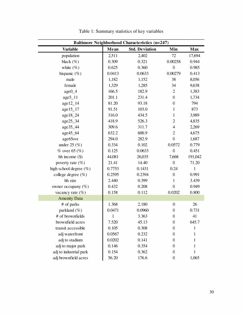
The first set of data we collect is socio-demographic information on the neighborhoods

themselves. Baltimore has 278 distinct city-defined neighborhoods of which 247 are residential

neighborhoods.2 The average population in each neighborhood is a little over 2,500 people. This

puts each neighborhood as roughly the same size as a U.S. Census Block Group but there is

tremendous variation in neighborhood size across the city. The largest single neighborhood,

Frankford, has over 17,000 residents according to the most recent U.S. Census estimates, while

the smallest, Blythewood had a population of just 72 people. We collect data on each

2 The remaining neighborhoods consist of industrial areas, large city parks, and one business park, all of which have no residents. These are dropped from our central analysis but create dummy variables for neighborhoods that border areas with brownfield sites, which include several industrial areas.

8

neighborhood’s residential composition, including racial and age breakdowns, in addition to data

on each neighborhoods housing stock, including vacancy rate. The source for this detailed

information in each neighborhood comes from the 2010 U.S. Census and from the five-year

American Community Survey (ACS) estimates spanning 2006-2010, created for the city due to a

special request from the Department of Planning to the Census Bureau. We provide a

comprehensive list of the socio-demographic data in Table 1 with key summary statistics.

The neighborhood data is nearly complete for all 247 residential neighborhoods but some

neighborhoods have key data necessary for our analysis missing. These include information on

the education level in each neighborhood from the ACS – percentage with high school degree or

higher and percentage with a bachelor’s degree or higher – which is missing from nine

neighborhoods and information on household income and the percentage of the population living

under the poverty line, missing from eight neighborhoods. Rather than drop these neighborhoods

from our analysis due to the missing data, we instead take a population weighted average of the

data from the surrounding neighborhoods and use this as an estimate for the missing data.

The second set of data we collect is amenity data for each neighborhood. We collect data

on the number of light-rail and subway stops in each neighborhood, the amount of parkland and

proximity to Baltimore’s largest parks and coastline, in addition to information on brownfields

within each neighborhood, and crime information. For the transportation data, we utilize GIS

shapefiles available from the Baltimore’s Open Data website and map light-rail and subway

locations to each neighborhood. We obtain a shapefile with all of the city maintained parks from

the same website and dissolve the park data layer into the neighborhood layer, which allows us

9

to calculate both the number of individual parks in each neighborhood and the percentage of

parkland per total area in the neighborhood.

For the brownfield data, we utilize the Brownfield Master Inventory (BMI), available

from the Maryland Department of the Environment. The BMI is the master list of all declared or

suspected – reported but not verified – brownfield sites in the entire state. We restrict our

brownfields of interest to only those within the City of Baltimore and utilize ArcGIS to geolocate

each of the sites in Baltimore into their requisite neighborhoods. We then tally the number of

brownfield sites in each neighborhood and the total acreage of all the sites. As shown in Table 1,

there is approximately one listed brownfields for every residential neighborhood in Baltimore,

with an average size per brownfield of 7.5 acres. All told, approximately 4.3% of all the non-

industrial land in Baltimore has brownfield status. This speaks both to the legacy of

environmental neglect in Baltimore but also to the systemic underlying environmental issues

pushing against efforts to revitalize city.

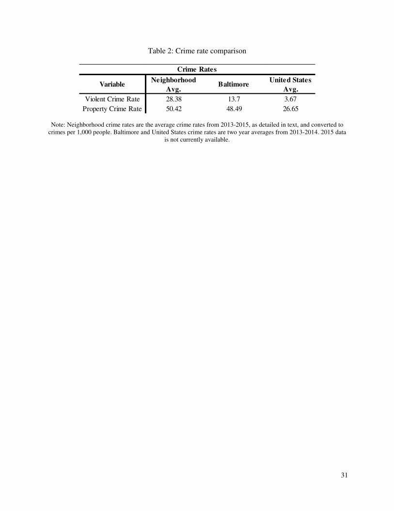
To calculate our crime rates, we collect the daily reported crime statistics for 2013

through 2015 from the Baltimore Police Department, which provides the type, date, and general

location of the crime, including the neighborhood. Baltimore Police define nine different types of

crimes with each type having several subcategories based on the crime itself. We follow

convention from the Federal Bureau of Investigation (United States Department of Justice, 2013)

and divide the nine types of crimes into two categories, violent and property crimes.3 We then

take the average of both crimes types over the three year period, divide by the neighborhood

3 Violent crimes consist of homicide, rape, robbery, and aggravated assault while property crimes consist of burglary, larceny, arson, and auto theft. The Baltimore crime statistics also have a miscellaneous category for shootings that do not fall under any other category. We do not include these as part of the violent crime category, in order to remain consistent with FBI guidelines. This means that the violent crime numbers are lower than they would be if miscellaneous shootings were included.

10

population, and multiply by 1,000 to standardize the crime rates.4 Table 2 provides some detail

on the crime rates in each neighborhood and compares the neighborhood average to the city’s

crime rates as a whole and to the U.S. crime rates. The differences in the neighborhood average

crime rates and the city-wide crime rates stem largely from the missing zero resident

neighborhoods, which have very low violent crime rates, as one would expect.

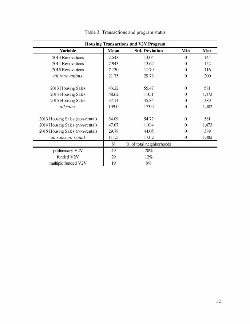
Our third set of collected data is information on housing sales5 and renovation activity

within Baltimore. We obtain housing sale records from 2013 through 2015 from Maryland

PropertyView, a database created by the Maryland Department of Planning that contains housing

and parcel information as well as GIS parcel data. We then geolocate each housing sale into its

requisite neighborhood and create a count of the housing sales per year in each neighborhood.

We are also able to distinguish between houses sold for owner occupancy versus houses sold as

rental properties from a unique identifier for the latter property type. The average neighborhood

had just under 22 housing renovations and 139 housing sales over our three year period, as seen

in table 3.

Similarly, we acquire all filed housing permits from the Housing Authority of Baltimore

City (HABC). This data includes the address of each permit in addition to the issue date, the

expiration date, and the neighborhood in which the address is located. Despite not explicitly

labeling the renovations by a unique code, we are able to identify renovation activity though the

permit description field which is the part of the physical permit where the work to be done is

described. Once we have created a short list of renovations, we match the addresses from the

4 We average the crime rates over a longer period in order to mitigate the effect of a spike in crime rates that occurred in 2015. We choose to use 1,000 instead of 100,000 as the means of standardizing the crime rates as our unit of observation is at a sub-city level. 5 Housing sales include detached single-family houses in addition to apartments, condominiums, and attached single-family house sales.

11

permit file to a master list of all housing parcels within Baltimore and retain only the renovation

activity that is matched to a residential parcel.6 As the V2V program is focused on revitalizing

neighborhoods through stimulating the housing market by removing excessive housing stock, we

want to examine the effect of the program on residential renovation activity only. This is not to

discount the possibility of V2V having a positive effect on non-residential renovation activity, as

it could lead to an increase in neighborhood desirability which would, in turn could cause

residents of the city to resort across neighborhoods. We leave this question open for future

research.

Our final set of data is on the V2V program itself. As mentioned in the previous sections,

the V2V program created a preliminary list of targeted areas in 2012 and funded a small set of

them in 2013 with additional areas funded in 2014. We tag each targeted area into its requisite

neighborhood and create a series of treatment groups based upon membership into the following

three groups: never neighborhoods, preliminary neighborhoods, and funded neighborhoods.

These are simply the neighborhoods that did not make the preliminary list, the neighborhoods

that made the list but were unfunded, and the neighborhoods funded at some point. We create an

additional set of dummy variables for neighborhoods that saw multiple V2V projects funded, as

seen in Table 3. All told, 49 neighborhoods made the short-list and 29 were funded during the

first two years7 of the program.

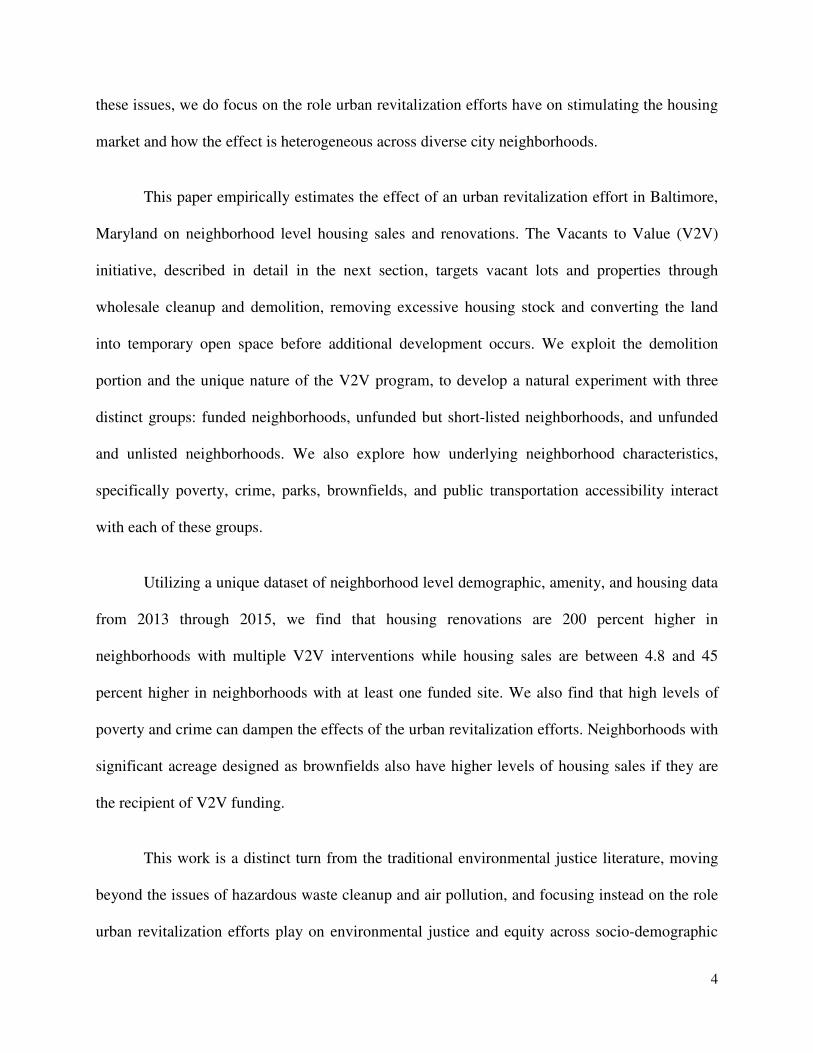
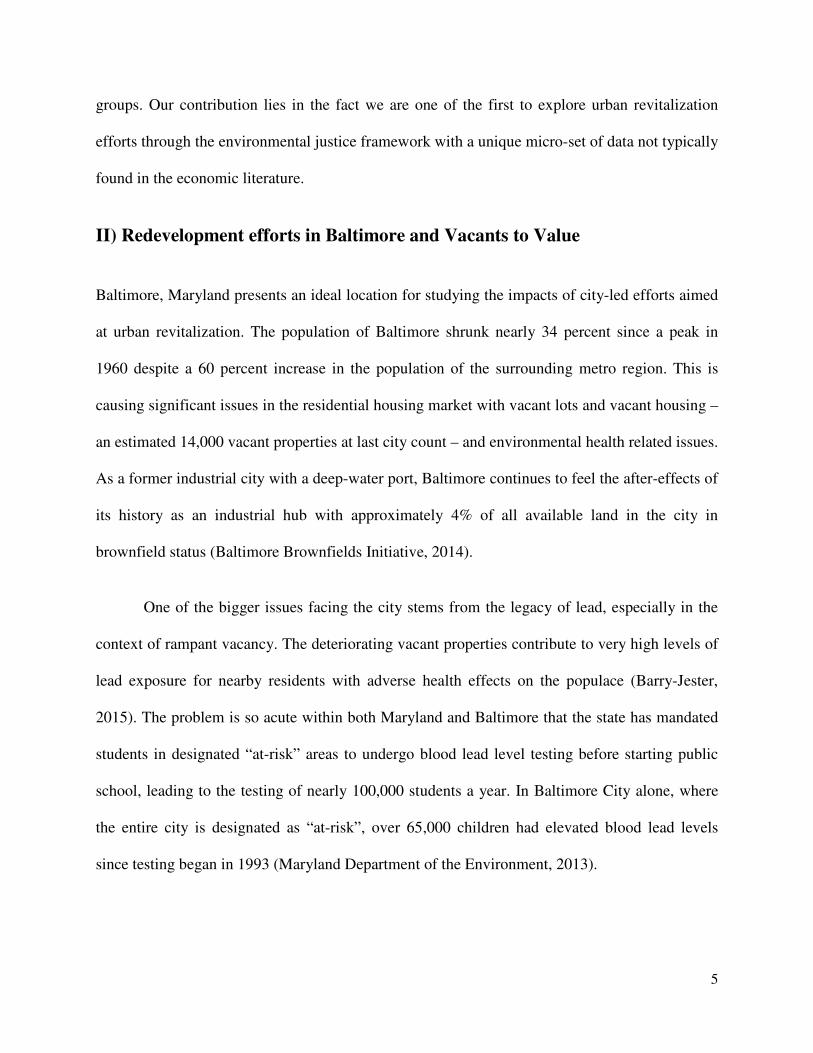
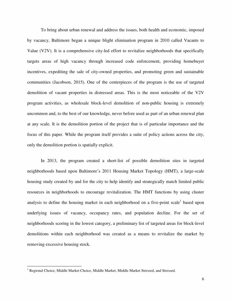
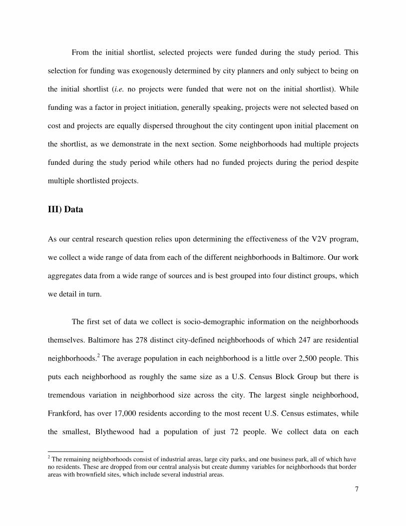
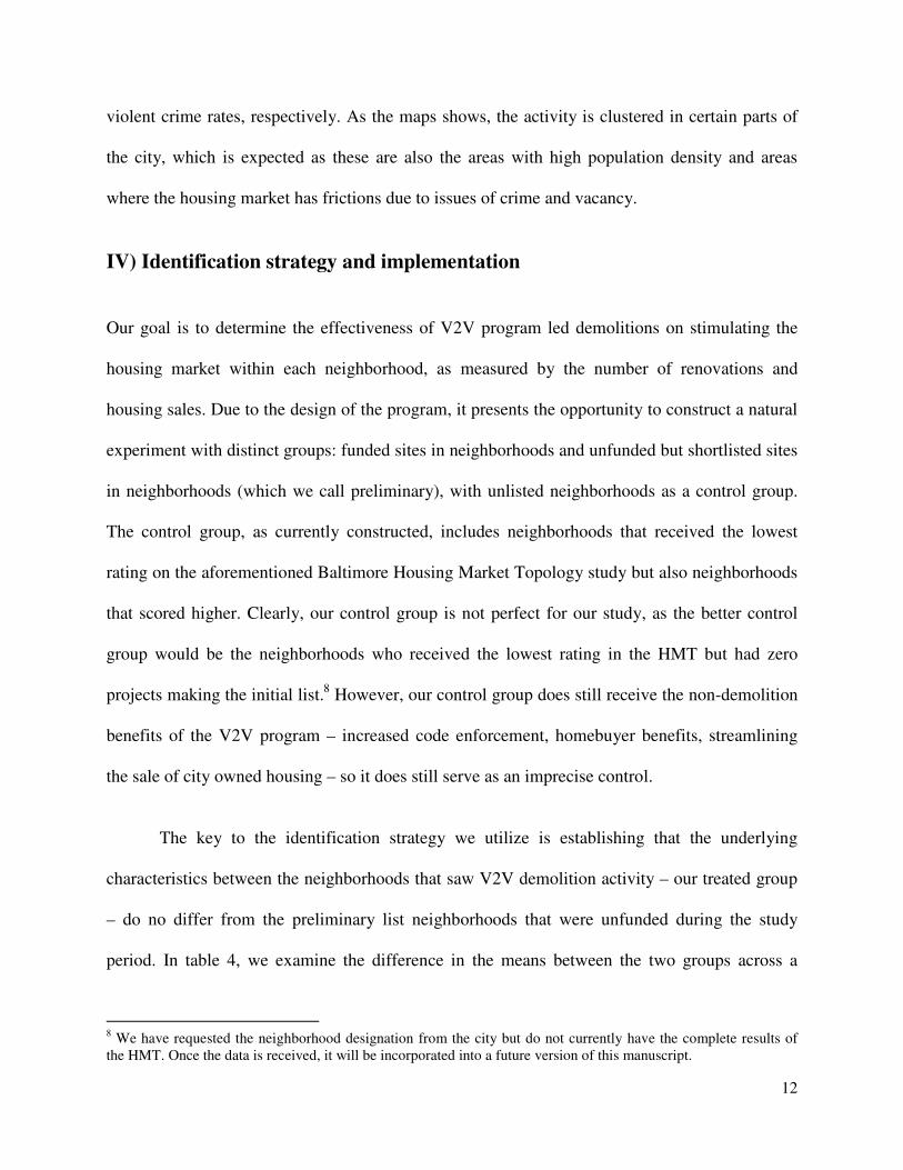
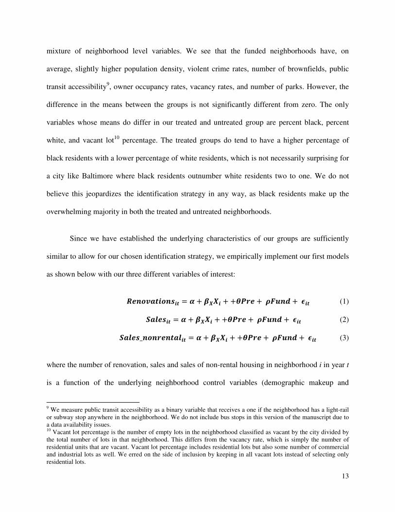
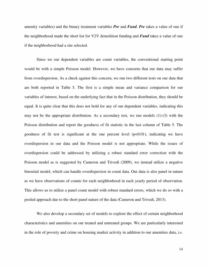
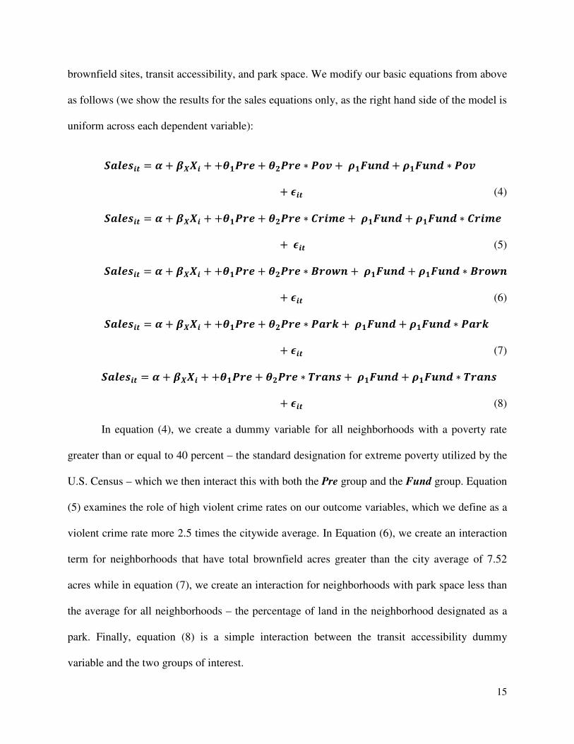
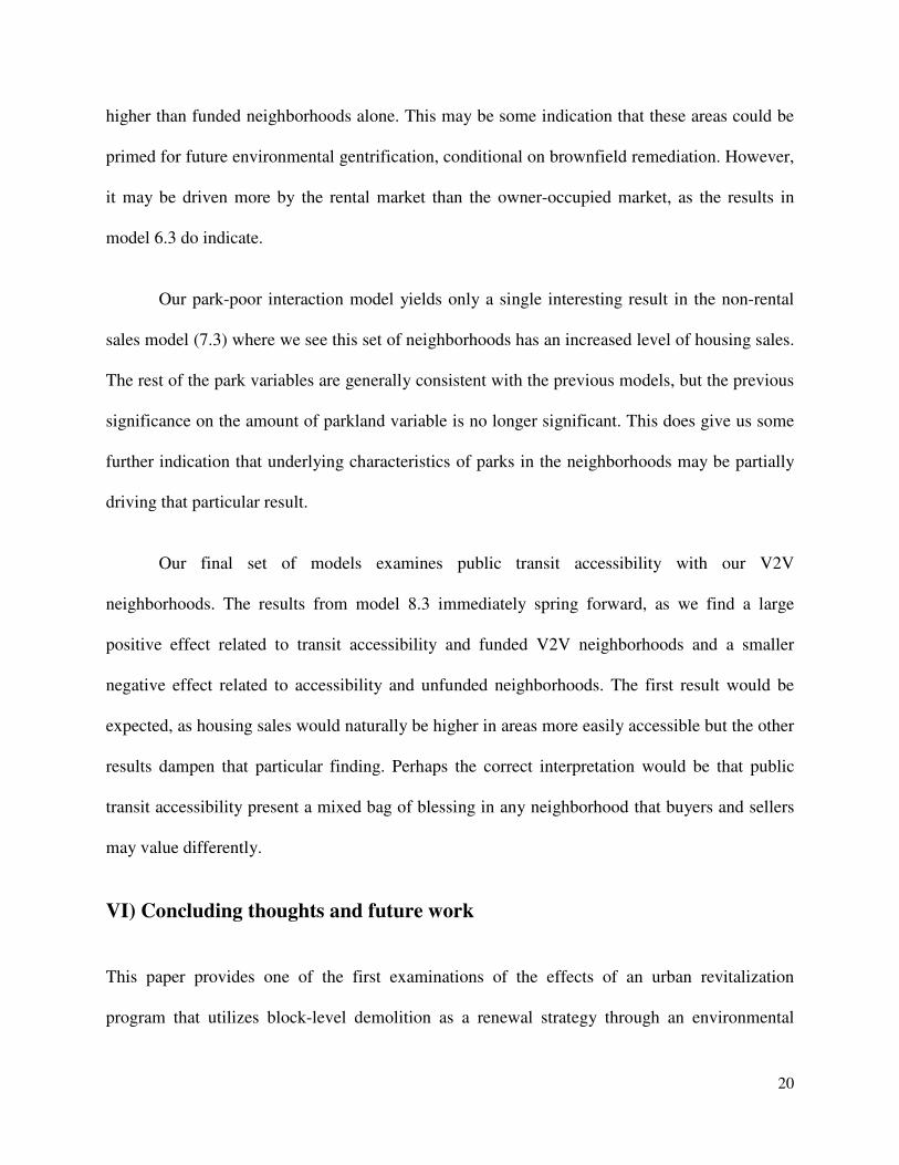
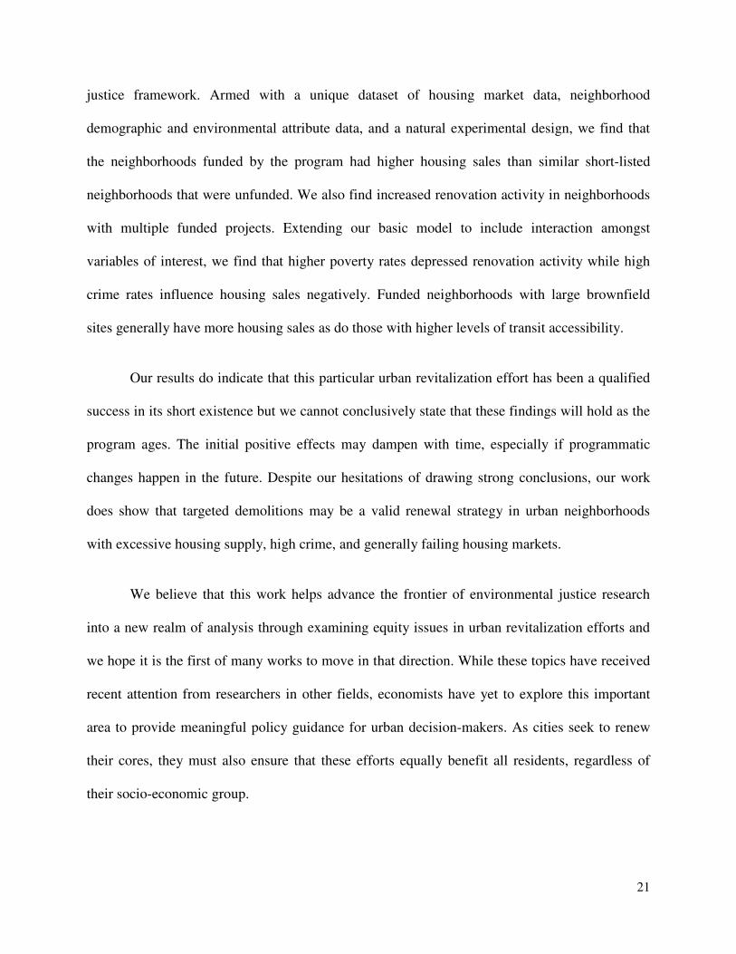
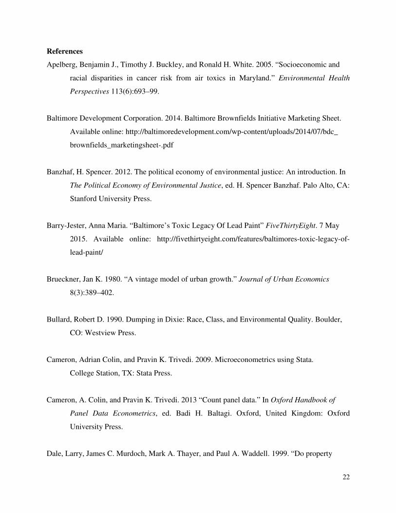
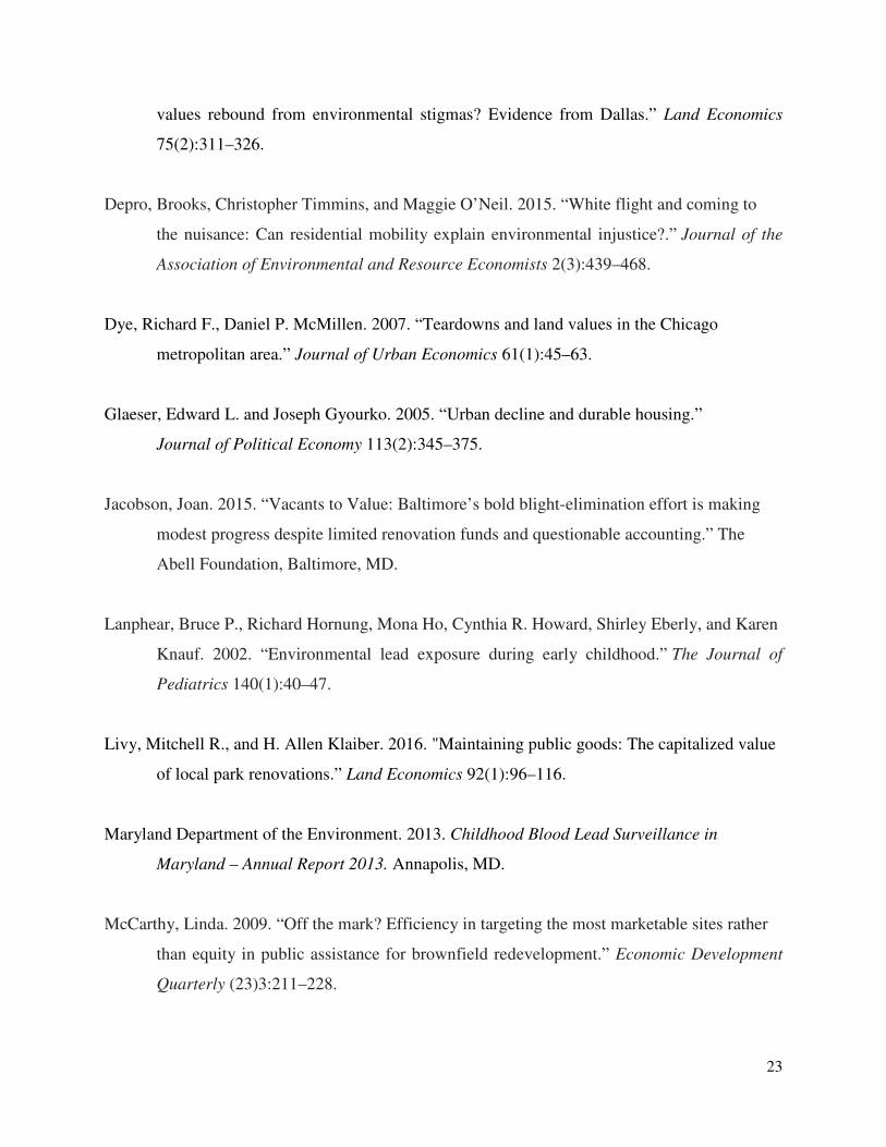
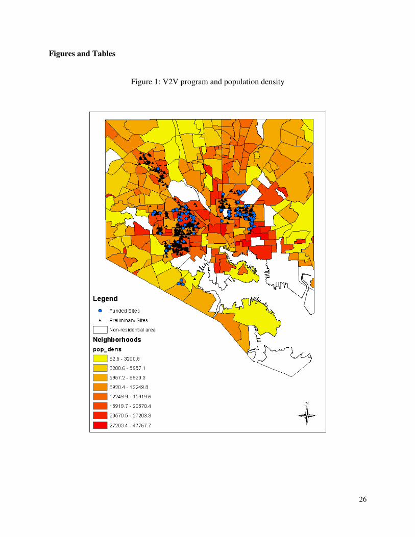
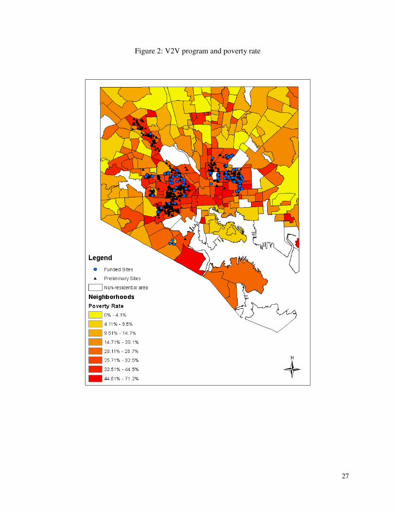
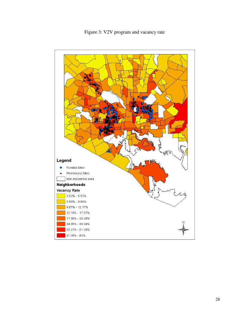
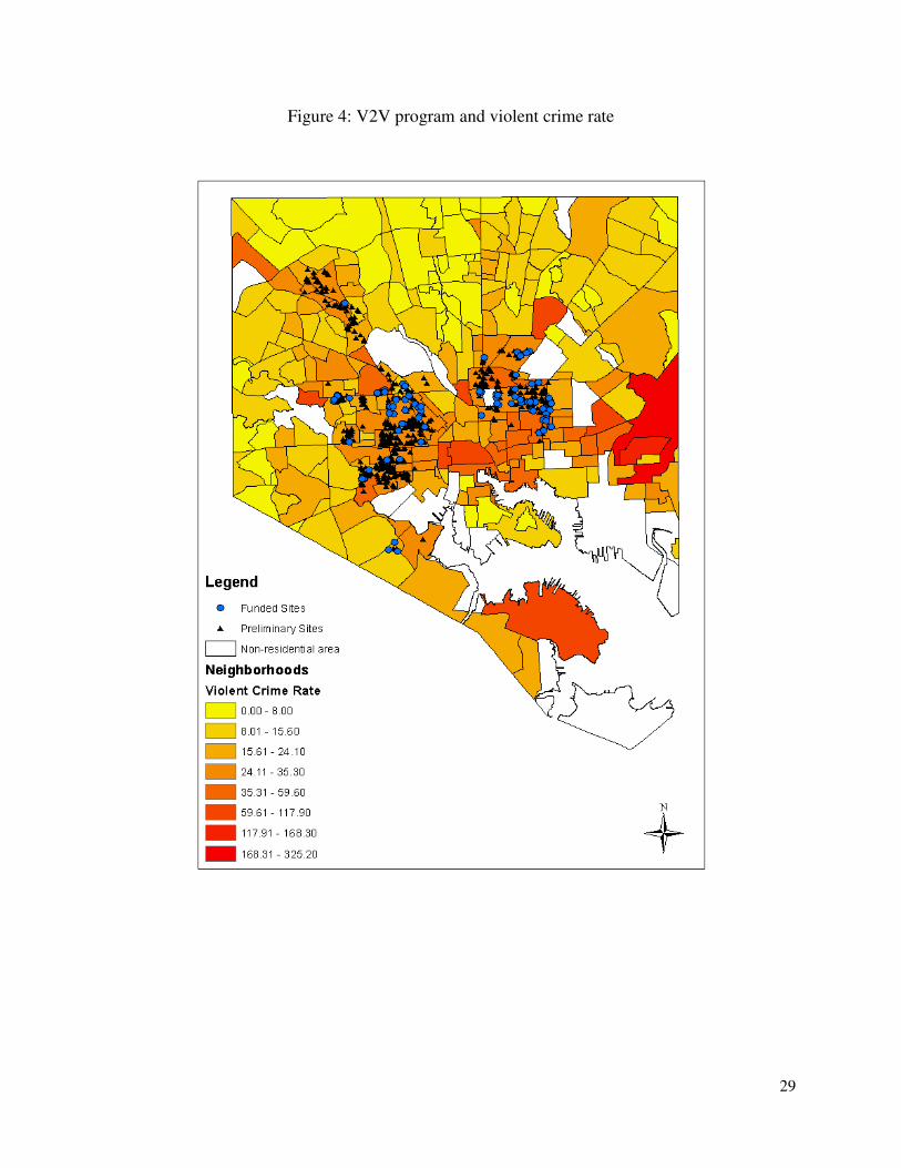
Figures 1-4 show the geographic distribution of the V2V activity across Baltimore, with

triangles indicating short-listed projects in each neighborhood and circles indicating funded

projects in each neighborhood and overlaid with population density, poverty, vacancy and

6 Housing renovations include the same property types gathered for housing sales. 7 Information on funding for 2015 is not currently available.

12

violent crime rates, respectively. As the maps shows, the activity is clustered in certain parts of

the city, which is expected as these are also the areas with high population density and areas

where the housing market has frictions due to issues of crime and vacancy.

IV) Identification strategy and implementation

Our goal is to determine the effectiveness of V2V program led demolitions on stimulating the

housing market within each neighborhood, as measured by the number of renovations and

housing sales. Due to the design of the program, it presents the opportunity to construct a natural

experiment with distinct groups: funded sites in neighborhoods and unfunded but shortlisted sites

in neighborhoods (which we call preliminary), with unlisted neighborhoods as a control group.

The control group, as currently constructed, includes neighborhoods that received the lowest

rating on the aforementioned Baltimore Housing Market Topology study but also neighborhoods

that scored higher. Clearly, our control group is not perfect for our study, as the better control

group would be the neighborhoods who received the lowest rating in the HMT but had zero

projects making the initial list.8 However, our control group does still receive the non-demolition

benefits of the V2V program – increased code enforcement, homebuyer benefits, streamlining

the sale of city owned housing – so it does still serve as an imprecise control.

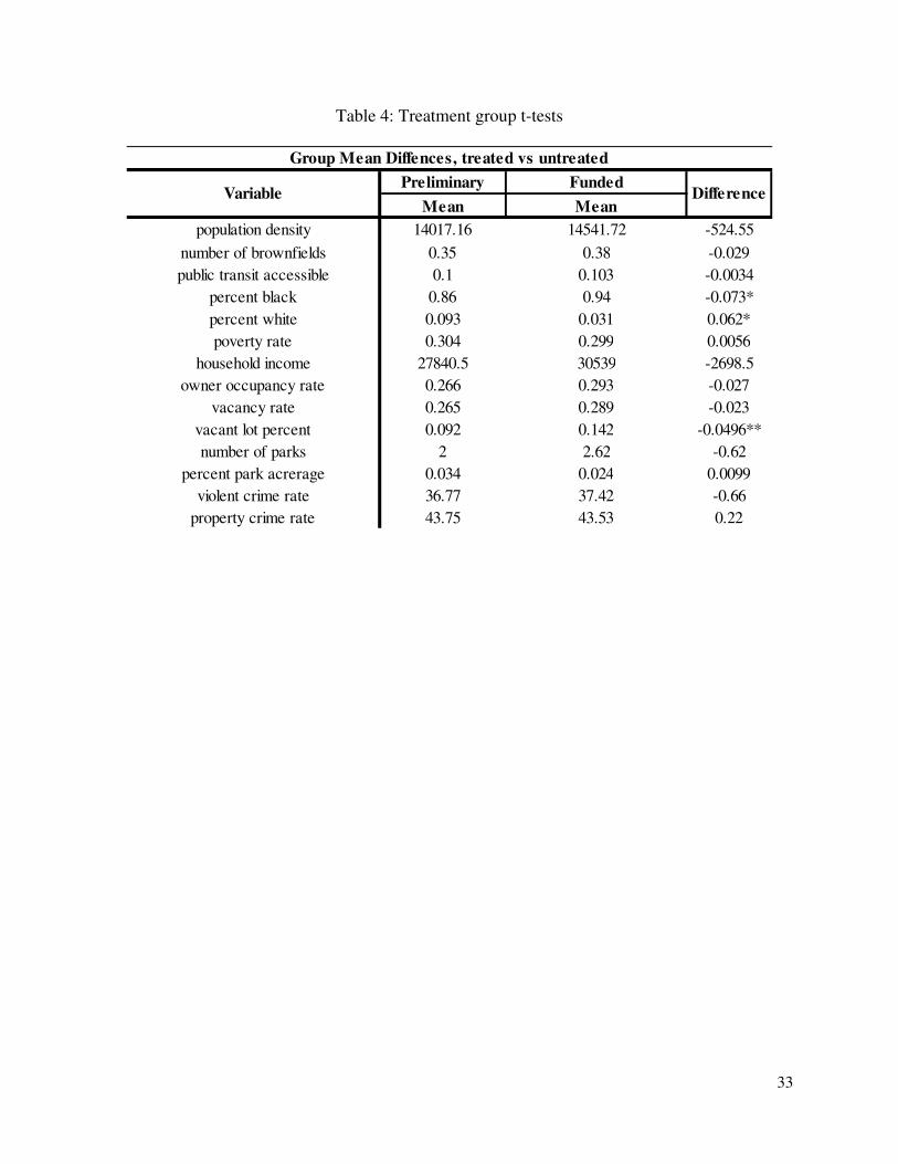
The key to the identification strategy we utilize is establishing that the underlying

characteristics between the neighborhoods that saw V2V demolition activity – our treated group

– do no differ from the preliminary list neighborhoods that were unfunded during the study

period. In table 4, we examine the difference in the means between the two groups across a

8 We have requested the neighborhood designation from the city but do not currently have the complete results of the HMT. Once the data is received, it will be incorporated into a future version of this manuscript.

13

mixture of neighborhood level variables. We see that the funded neighborhoods have, on

average, slightly higher population density, violent crime rates, number of brownfields, public

transit accessibility9, owner occupancy rates, vacancy rates, and number of parks. However, the

difference in the means between the groups is not significantly different from zero. The only

variables whose means do differ in our treated and untreated group are percent black, percent

white, and vacant lot10 percentage. The treated groups do tend to have a higher percentage of

black residents with a lower percentage of white residents, which is not necessarily surprising for

a city like Baltimore where black residents outnumber white residents two to one. We do not

believe this jeopardizes the identification strategy in any way, as black residents make up the

overwhelming majority in both the treated and untreated neighborhoods.

Since we have established the underlying characteristics of our groups are sufficiently

similar to allow for our chosen identification strategy, we empirically implement our first models

as shown below with our three different variables of interest:

!"#$%&'($#)(' = + + -..( + +/01" + 345#6 +7(' (1)

8&9")(' = + + -..( + +/01" + 345#6 +7(' (2)

8&9")_#$#1"#'&9(' = + + -..( + +/01" + 345#6 +7(' (3)

where the number of renovation, sales and sales of non-rental housing in neighborhood i in year t

is a function of the underlying neighborhood control variables (demographic makeup and

9 We measure public transit accessibility as a binary variable that receives a one if the neighborhood has a light-rail or subway stop anywhere in the neighborhood. We do not include bus stops in this version of the manuscript due to a data availability issues. 10 Vacant lot percentage is the number of empty lots in the neighborhood classified as vacant by the city divided by the total number of lots in that neighborhood. This differs from the vacancy rate, which is simply the number of residential units that are vacant. Vacant lot percentage includes residential lots but also some number of commercial and industrial lots as well. We erred on the side of inclusion by keeping in all vacant lots instead of selecting only residential lots.

14

amenity variables) and the binary treatment variables Pre and Fund. Pre takes a value of one if

the neighborhood made the short list for V2V demolition funding and Fund takes a value of one

if the neighborhood had a site selected.

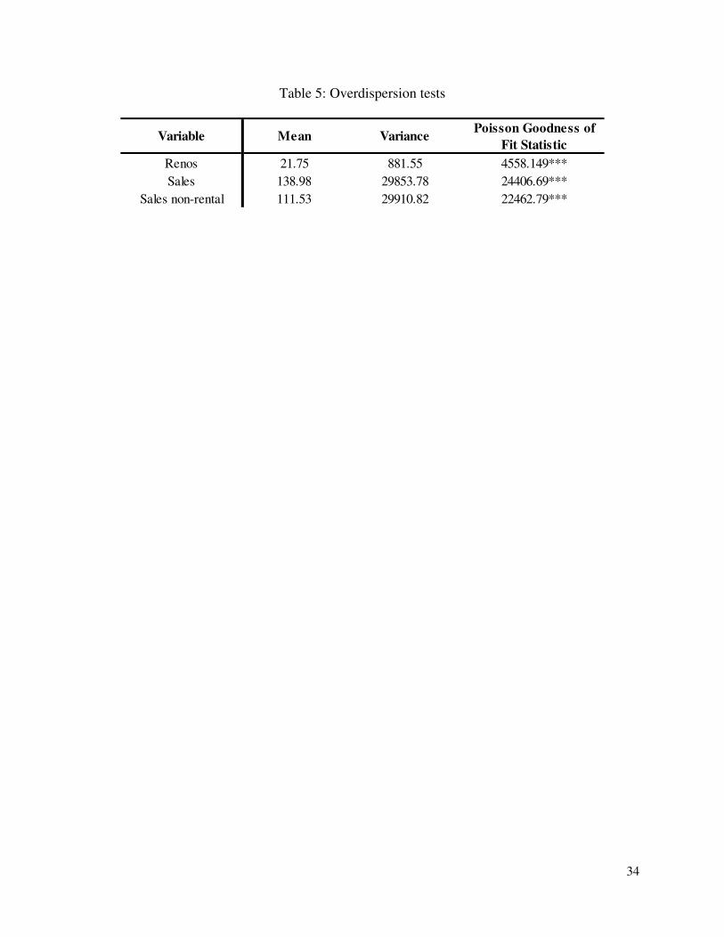
Since we our dependent variables are count variables, the conventional starting point

would be with a simple Poisson model. However, we have concerns that our data may suffer

from overdispersion. As a check against this concern, we run two different tests on our data that

are both reported in Table 5. The first is a simple mean and variance comparison for our

variables of interest, based on the underlying fact that in the Poisson distribution, they should be

equal. It is quite clear that this does not hold for any of our dependent variables, indicating this

may not be the appropriate distribution. As a secondary test, we run models (1)-(3) with the

Poisson distribution and report the goodness of fit statistic in the last column of Table 5. The

goodness of fit test is significant at the one percent level (p<0.01), indicating we have

overdispersion in our data and the Poisson model is not appropriate. While the issues of

overdispersion could be addressed by utilizing a robust standard error correction with the

Poisson model as is suggested by Cameron and Trivedi (2009), we instead utilize a negative

binomial model, which can handle overdispersion in count data. Our data is also panel in nature

as we have observations of counts for each neighborhood in each yearly period of observation.

This allows us to utilize a panel count model with robust standard errors, which we do so with a

pooled approach due to the short panel nature of the data (Cameron and Trivedi, 2013).

We also develop a secondary set of models to explore the effect of certain neighborhood

characteristics and amenities on our treated and untreated groups. We are particularly interested

in the role of poverty and crime on housing market activity in addition to our amenities data, i.e.

15

brownfield sites, transit accessibility, and park space. We modify our basic equations from above

as follows (we show the results for the sales equations only, as the right hand side of the model is

uniform across each dependent variable):

8&9")(' = + + -..( + +/;01" + /<01" ∗ 0$% +3;45#6 + 3;45#6 ∗ 0$%

+7(' (4)

8&9")(' = + + -..( + +/;01" + /<01" ∗ >1(?" +3;45#6 + 3;45#6 ∗ >1(?"

+7(' (5)

8&9")(' = + + -..( + +/;01" + /<01" ∗ @1$A# +3;45#6 + 3;45#6 ∗ @1$A#

+7(' (6)

8&9")(' = + + -..( + +/;01" + /<01" ∗ 0&1B +3;45#6 + 3;45#6 ∗ 0&1B

+7(' (7)

8&9")(' = + + -..( + +/;01" + /<01" ∗ C1&#) +3;45#6 + 3;45#6 ∗ C1&#)

+7(' (8)

In equation (4), we create a dummy variable for all neighborhoods with a poverty rate

greater than or equal to 40 percent – the standard designation for extreme poverty utilized by the

U.S. Census – which we then interact this with both the Pre group and the Fund group. Equation

(5) examines the role of high violent crime rates on our outcome variables, which we define as a

violent crime rate more 2.5 times the citywide average. In Equation (6), we create an interaction

term for neighborhoods that have total brownfield acres greater than the city average of 7.52

acres while in equation (7), we create an interaction for neighborhoods with park space less than

the average for all neighborhoods – the percentage of land in the neighborhood designated as a

park. Finally, equation (8) is a simple interaction between the transit accessibility dummy

variable and the two groups of interest.

16

V) Estimation results and discussion

We estimate the first set of models in Table 6, which arise from equations 1-3. Focusing first on

model 1 and on our variables of interest, we find that neighborhoods designated on the short list

for V2V funding see no effect on the total number of housing renovations. We also find that our

treated group, the funded neighborhoods, likewise sees no effect on the renovation level. We do

see a strong positive effect for a subgroup of our main treated variable, the neighborhoods that

had multiple V2V projects funded. For this group, we find that housing renovations increased by

200 percent11 for this set of neighborhoods. This particular result indicates that renovation

activity may not be spurred along by a simple one-time investment into the neighborhood by the

city, as it may not be a sufficient signal to spur homeowner reinvestment in their own property.

Rather, the stronger signal of multiple occurrences of investment indicates that the city is

sufficiently investing into the area rather than a simple one-off event.

In model 2, our outcome variable changes to the number of housing sales in each

neighborhood and we see a similar story as before with the preliminary group seeing no effect

from making the short list. We do find a positive result significant at the five percent level with

funded projects, with housing sales in these neighborhoods up by over 45 percent with no

additional effect found for multiple project neighborhoods. Model 2 indicates that the V2V

program may be spurring a housing market turnaround as intended.

The results of non-rental housing sales in model 3 paints a more complicated story, as

here we find statistically significant results for both the preliminary and funded groups, at the

one and ten percent levels, respectively, but with point estimates in the opposite directions.

11 Using the standard conversion of e^(coefficient).

17

Neighborhoods on the initial list see non-rental housing sales that are 69.3 percent lower than

non-short listed neighborhoods but that effect is reversed for those neighborhoods that have a

funded project. Here, housing sales are 74.1 percent higher, which means the net effect in these

neighborhoods would be a 4.8 percent increase in housing sales. The total effect is an order of

magnitude lower than the model that looks at all housing sales12 but is still indicative of the V2V

project stimulating demand in the market in these neighborhoods. However, all is not well in the

non-funded markets, as they do not receive the positive funding effect offset thus housing sales

are just generally depressed in that area, conditional on initial list placement. If we interpret this

result from an individual asset holder’s perspective – the homeowner – the decrease in housing

sales makes intuitive sense. If one expects that the value of your asset may increase in the future,

say for example by an increased demand for housing as supply decreases via demolitions, that

asset would be held into the next period. Therefore, homeowners may simply be waiting for

clarity on the location of future V2V projects.

We now turn to discussing the results from a select number of the control variables from

all three of the previous models, starting with the sociodemographic variables. We find that

poverty rate is negative and statistically significant at high levels in all of our models. A one-unit

change in the poverty rate in a neighborhood leads to 1.265 percent change in the number of

renovations, a 0.176 percent change in housing sales, and a 0.415 percent change in non-rental

housing sales. We see similar outcomes with the violent crime rate, but with a bigger effect on

the sales models. Intuitively, this makes sense, as high crime areas are less attractive to

prospective homebuyers. We also see a marked difference in the point estimates between all

housing sales and non-rental housing sales.

12 As with many cities, Baltimore has a large rental market, so it would be expected that rental investment groups would attempt to buy into areas of the city where they expect future land rents to increase.

18

Curiously, we see a positive effect for housing vacancy in all of the models, with a large

effect in the renovation model. Though this may be counter to initial expectations, it could be

partially explained by an increased number of residential units available for renovation or sale at

a discounted or some underlying differences in housing values in each neighborhood not

accounted for in our models. Further work may be warranted to explain this strange result.

Moving to the amenities and environmental control variables, we do not find a consistent

effect for transportation accessibility across the models. For the case of stadium13 proximity, we

see a negative effect for both housing sales models, possibly driven by congestion and noise

effects of a busy area. We find an interesting and mixed set of results for parks, with a single

positive effect in the all-sales model for proximity to one of Baltimore’s major parks but no

effect in the non-rental sales model. The number of parks in a neighborhood corresponds to an

increase in both renovations and sales but the effect of the amount of parkland is actually

negative across all models. At best, this paints an interesting picture of differential effects of

parks between neighborhoods. These effects may be driven by the data construction, as we treat

all parks as equal in the parks variable, which may not hold in all cases, given the result from the

major park adjacency variable. Underlying park-level attributes have been shown to affect the

value of parks in previous work (see Livy and Klaiber, 2016). With the brownfield variables, we

find only a single consistently significant variable across all models, which is the number of

brownfield acres in each neighborhood. Curiously, the sign flips from negative in the renovation

model to positive in the sales models.

V.i) Interaction model results and discussion

13 The stadiums are Camden Yards, home of the Baltimore Orioles, and M&T Bank Stadium, home of the Baltimore Ravens. Both are located in the same neighborhood, which is non-residential with a heavy commercial component.

19

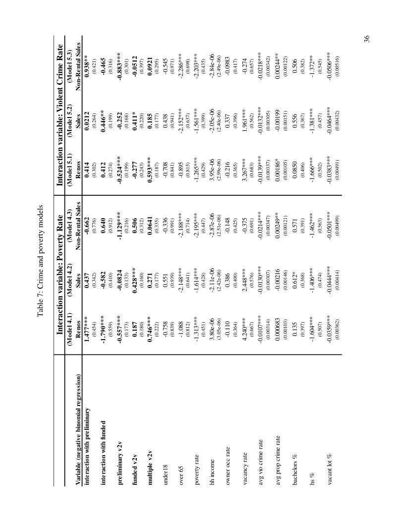
We report the results of equations (4) and (5) in Table 7. We group the each of the equations

together in the table, thus models 4.1 through 4.3 utilize equation (4) each with a different

dependent variable while models 5.1 through 5.3 utilize equation (5) in a similar manner. With

our poverty interaction models, we only find significant results on our interaction variables with

renovations. Our previous finding that renovations are over 200 percent higher in neighborhoods

with multiple funded projects remains but a few curious results crop up on the interaction terms.

Both are significant at the one percent level but point in different directions. High poverty

neighborhoods on the preliminary list see 438 percent higher levels of renovations but funded

projects in these areas have 83 percent lower renovations. Considering we do not see similar

behavior in the companion sales models, these results are likely spurious and an artifact of the

data.

On the crime interaction models, we find two significant results, both at the five percent

level and both in one of the sales models. In the all-sales model (5.2), high violent crime

neighborhoods that have funded V2V projects see a 56 percent increase in housing sales. This

effect is large enough to offset the general decline in sales found in our earlier models. In the

non-rental sales model (5.3), we find a large effect associated with the preliminary listed high

crime neighborhoods. Both results give some indication that the V2V program may be improving

the housing market in these high crime areas if but only marginally.

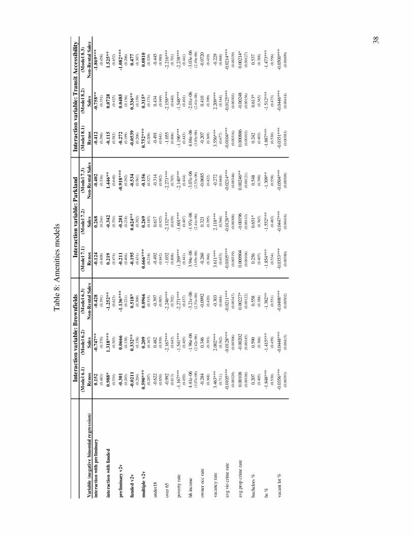
In our first set of amenity models, we model interactions with V2V neighborhoods and

neighborhoods with higher than average brownfield acreage. In the all-sales model (6.2), we find

that the interaction of our treated group has a large value that is significant at the one percent

level. This set of neighborhoods has house sales that are 373 percent higher and over 300 percent

20

higher than funded neighborhoods alone. This may be some indication that these areas could be

primed for future environmental gentrification, conditional on brownfield remediation. However,

it may be driven more by the rental market than the owner-occupied market, as the results in

model 6.3 do indicate.

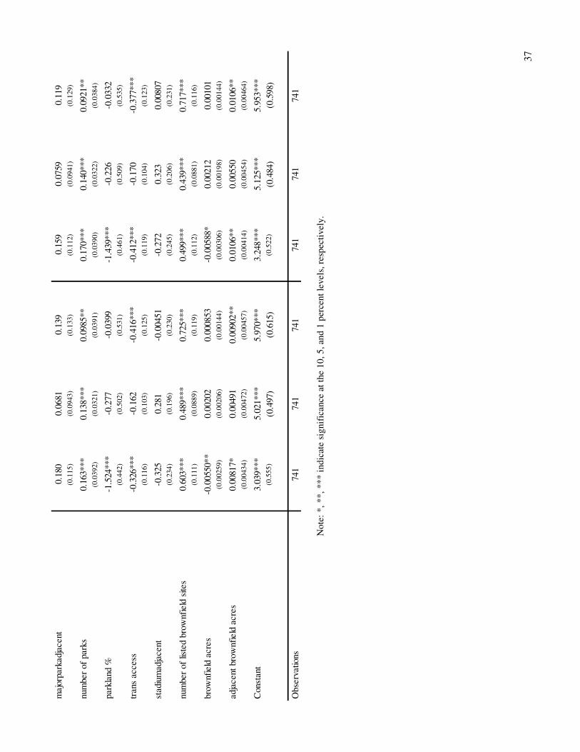
Our park-poor interaction model yields only a single interesting result in the non-rental

sales model (7.3) where we see this set of neighborhoods has an increased level of housing sales.

The rest of the park variables are generally consistent with the previous models, but the previous

significance on the amount of parkland variable is no longer significant. This does give us some

further indication that underlying characteristics of parks in the neighborhoods may be partially

driving that particular result.

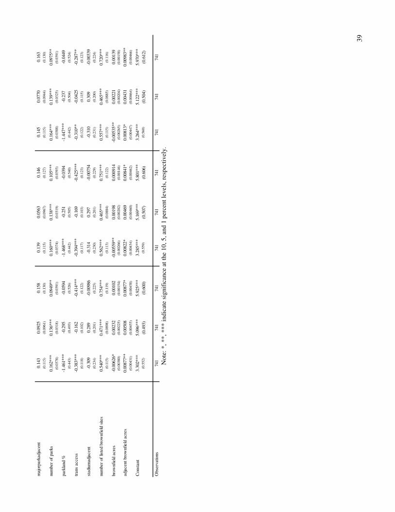
Our final set of models examines public transit accessibility with our V2V

neighborhoods. The results from model 8.3 immediately spring forward, as we find a large

positive effect related to transit accessibility and funded V2V neighborhoods and a smaller

negative effect related to accessibility and unfunded neighborhoods. The first result would be

expected, as housing sales would naturally be higher in areas more easily accessible but the other

results dampen that particular finding. Perhaps the correct interpretation would be that public

transit accessibility present a mixed bag of blessing in any neighborhood that buyers and sellers

may value differently.

VI) Concluding thoughts and future work

This paper provides one of the first examinations of the effects of an urban revitalization

program that utilizes block-level demolition as a renewal strategy through an environmental

21

justice framework. Armed with a unique dataset of housing market data, neighborhood

demographic and environmental attribute data, and a natural experimental design, we find that

the neighborhoods funded by the program had higher housing sales than similar short-listed

neighborhoods that were unfunded. We also find increased renovation activity in neighborhoods

with multiple funded projects. Extending our basic model to include interaction amongst

variables of interest, we find that higher poverty rates depressed renovation activity while high

crime rates influence housing sales negatively. Funded neighborhoods with large brownfield

sites generally have more housing sales as do those with higher levels of transit accessibility.

Our results do indicate that this particular urban revitalization effort has been a qualified

success in its short existence but we cannot conclusively state that these findings will hold as the

program ages. The initial positive effects may dampen with time, especially if programmatic

changes happen in the future. Despite our hesitations of drawing strong conclusions, our work

does show that targeted demolitions may be a valid renewal strategy in urban neighborhoods

with excessive housing supply, high crime, and generally failing housing markets.

We believe that this work helps advance the frontier of environmental justice research

into a new realm of analysis through examining equity issues in urban revitalization efforts and

we hope it is the first of many works to move in that direction. While these topics have received

recent attention from researchers in other fields, economists have yet to explore this important

area to provide meaningful policy guidance for urban decision-makers. As cities seek to renew

their cores, they must also ensure that these efforts equally benefit all residents, regardless of

their socio-economic group.

22

References

Apelberg, Benjamin J., Timothy J. Buckley, and Ronald H. White. 2005. “Socioeconomic and

racial disparities in cancer risk from air toxics in Maryland.” Environmental Health

Perspectives 113(6):693–99.

Baltimore Development Corporation. 2014. Baltimore Brownfields Initiative Marketing Sheet.

Available online: http://baltimoredevelopment.com/wp-content/uploads/2014/07/bdc_

brownfields_marketingsheet-.pdf

Banzhaf, H. Spencer. 2012. The political economy of environmental justice: An introduction. In

The Political Economy of Environmental Justice, ed. H. Spencer Banzhaf. Palo Alto, CA:

Stanford University Press.

Barry-Jester, Anna Maria. “Baltimore’s Toxic Legacy Of Lead Paint” FiveThirtyEight. 7 May

2015. Available online: http://fivethirtyeight.com/features/baltimores-toxic-legacy-of-

lead-paint/

Brueckner, Jan K. 1980. “A vintage model of urban growth.” Journal of Urban Economics

8(3):389–402.

Bullard, Robert D. 1990. Dumping in Dixie: Race, Class, and Environmental Quality. Boulder,

CO: Westview Press.

Cameron, Adrian Colin, and Pravin K. Trivedi. 2009. Microeconometrics using Stata.

College Station, TX: Stata Press.

Cameron, A. Colin, and Pravin K. Trivedi. 2013 “Count panel data.” In Oxford Handbook of

Panel Data Econometrics, ed. Badi H. Baltagi. Oxford, United Kingdom: Oxford

University Press.

Dale, Larry, James C. Murdoch, Mark A. Thayer, and Paul A. Waddell. 1999. “Do property

23

values rebound from environmental stigmas? Evidence from Dallas.” Land Economics

75(2):311–326.

Depro, Brooks, Christopher Timmins, and Maggie O’Neil. 2015. “White flight and coming to

the nuisance: Can residential mobility explain environmental injustice?.” Journal of the

Association of Environmental and Resource Economists 2(3):439–468.

Dye, Richard F., Daniel P. McMillen. 2007. “Teardowns and land values in the Chicago

metropolitan area.” Journal of Urban Economics 61(1):45–63.

Glaeser, Edward L. and Joseph Gyourko. 2005. “Urban decline and durable housing.”

Journal of Political Economy 113(2):345–375.

Jacobson, Joan. 2015. “Vacants to Value: Baltimore’s bold blight-elimination effort is making

modest progress despite limited renovation funds and questionable accounting.” The

Abell Foundation, Baltimore, MD.

Lanphear, Bruce P., Richard Hornung, Mona Ho, Cynthia R. Howard, Shirley Eberly, and Karen

Knauf. 2002. “Environmental lead exposure during early childhood.” The Journal of

Pediatrics 140(1):40–47.

Livy, Mitchell R., and H. Allen Klaiber. 2016. "Maintaining public goods: The capitalized value

of local park renovations.” Land Economics 92(1):96–116.

Maryland Department of the Environment. 2013. Childhood Blood Lead Surveillance in

Maryland – Annual Report 2013. Annapolis, MD.

McCarthy, Linda. 2009. “Off the mark? Efficiency in targeting the most marketable sites rather

than equity in public assistance for brownfield redevelopment.” Economic Development

Quarterly (23)3:211–228.

24

McCluskey, Jill J. and Gordon C. Rausser, 2001. “Estimation of perceived risk and its effect on

property values.” Land Economics 77(1):42–55.

McCluskey, Jill J. & Rausser, Gordon C., 2003. “Hazardous waste sites and housing

appreciation rates.” Journal of Environmental Economics and Management 45(2):166–

176.

McMillen, Daniel P. and Arthur O’Sullivan. 2013. “Option value and the price of teardown

properties.” Journal of Urban Economics 74(1):71–82.

Oakes, John M., Douglas L. Anderton, and Andy B. Anderson. 1996. “A longitudinal analysis of

environmental equity in communities with hazardous waste facilities.” Social Science

Research 25:125–48.

Pastor, Manuel, Jim Sadd, and John Hipp. 2001. “Which came first? Toxic facilities, minority

move‐in, and environmental justice.” Journal of Urban Affairs 23(1):1–21.

Rosenthal, Stuart S. and Robert W. Helsley. 1994. “Redevelopment and the urban land price

gradient.” Journal of Urban Economics 35(2):182–200.

Rosenthal, Stuart S. 2008. “Old homes, externalities, and poor neighborhoods: A dynamic

model of urban decline and renewal.” Journal of Urban Economics 633(3):816–840.

Schoenbaum, Miriam. 2002. “Environmental contamination, brownfields policy, and economic

redevelopment in an industrial area of Baltimore, Maryland.” Land Economics 78(1):60-

71.

Sayre, James W., and Monica D. Katzel. 1979. “Household surface lead dust: Its accumulation in

vacant homes.” Environmental Health Perspectives 29:179-182.

Schweitzer, Lisa, and Max Stephenson. 2007. “Right answers, wrong questions: environmental

25

justice as urban research.” Urban Studies 44(2):319–337.

Silverman, Robert, Li Yin, and Kelly L. Patterson. 2013. “Dawn of the dead city: An exploratory

analysis of vacant addresses in Buffalo, NY 2008–2010.” Journal of Urban

Affairs 35(2):131–152.

United Church of Christ (UCC), Commission for Racial Justice. 1987. “Toxic wastes and race in

the United States: A national report on the racial and socio-economic characteristics of

communities with hazardous waste sites.” New York: Public Data Access, Inc.

United States Department of Justice, Federal Bureau of Investigation. 2013. Crime in

the United States, 2012.

Wheaton, William C. 1982. “Urban spatial development with durable but replaceable capital.”

Journal of Urban Economics 12(1):53–67.

Wilson, Sacoby, Malo Hutson, and Mahasin Mujahid. 2008. “How planning and zoning

contribute to inequitable development, neighborhood health, and environmental

injustice.” Environmental Justice 1(4):211–216.

Viscusi, W. Kip, and Hamilton James T. 1999. “Are risk regulators rational? Evidence from

hazardous waste cleanup decisions.” The American Economic Review 89(4):1010–1027.

26

Figures and Tables

Figure 1: V2V program and population density

27

Figure 2: V2V program and poverty rate

28

Figure 3: V2V program and vacancy rate

29

Figure 4: V2V program and violent crime rate

30

Table 1: Summary statistics of key variables

Variable Mean Std. Deviation Min Max

population 2,511 2,402 72 17,694

black (%) 0.309 0.321 0.00258 0.944

white (%) 0.625 0.360 0 0.985

hispanic (%) 0.0413 0.0633 0.00279 0.413

male 1,182 1,152 38 8,056

female 1,329 1,285 34 9,638

age0_4 166.5 182.9 2 1,383

age5_11 201.1 231.4 0 1,734

age12_14 81.20 93.18 0 794

age15_17 91.51 103.0 1 873

age18_24 316.0 434.5 1 3,989

age25_34 418.9 526.3 2 4,835

age35_44 309.6 311.7 4 2,269

age45_64 632.2 600.9 2 4,675

age65ovr 294.0 282.9 0 1,687

under 25 (%) 0.334 0.102 0.0572 0.779

% over 65 (%) 0.125 0.0633 0 0.451

hh income ($) 44,081 26,035 7,668 191,042

poverty rate (%) 21.41 14.40 0 71.20

high school degree (%) 0.7753 0.1431 0.24 1

college degree (%) 0.2595 0.2394 0 0.991

hh size 2.440 0.399 1 3.439

owner occupany (%) 0.432 0.208 0 0.949

vacancy rate (%) 0.158 0.112 0.0202 0.800

Amenity Data

# of parks 1.368 2.180 0 26

parkland (%) 0.0471 0.0960 0 0.731

# of brownfields 1 3.363 0 41

brownfield acres 7.520 45.13 0 645.7

transit accessible 0.105 0.308 0 1

adj waterfront 0.0567 0.232 0 1

adj to stadium 0.0202 0.141 0 1

adj to major park 0.146 0.354 0 1

adj to industrial park 0.154 0.362 0 1

adj brownfield acres 56.20 176.6 0 1,065

Baltimore Neighborhood Characteristics (n=247)

31

Table 2: Crime rate comparison

Note: Neighborhood crime rates are the average crime rates from 2013-2015, as detailed in text, and converted to crimes per 1,000 people. Baltimore and United States crime rates are two year averages from 2013-2014. 2015 data

is not currently available.

VariableNeighborhood

Avg.Baltimore

United States

Avg.

Violent Crime Rate 28.38 13.7 3.67

Property Crime Rate 50.42 48.49 26.65

Crime Rates

32

Table 3: Transactions and program status

Variable Mean Std. Deviation Min Max

2013 Renovations 7.543 13.04 0 145

2014 Renovations 7.943 13.62 0 152

2015 Renovations 7.130 11.79 0 116

all renovations 21.75 29.73 0 200

2013 Housing Sales 43.22 55.47 0 581

2014 Housing Sales 58.62 110.1 0 1,473

2015 Housing Sales 37.14 45.84 0 389

all sales 139.0 173.0 0 1,482

2013 Housing Sales (non-rental) 34.09 54.72 0 581

2014 Housing Sales (non-rental) 47.67 110.4 0 1,473

2015 Housing Sales (non-rental) 29.78 44.05 0 389

all sales no rental 111.5 173.2 0 1,482

N % of total neighborhoods

preliminary V2V 49 20%

funded V2V 29 12%

multiple funded V2V 19 8%

Housing Transactions and V2V Program

33

Table 4: Treatment group t-tests

Preliminary Funded

Mean Mean

population density 14017.16 14541.72 -524.55

number of brownfields 0.35 0.38 -0.029

public transit accessible 0.1 0.103 -0.0034

percent black 0.86 0.94 -0.073*

percent white 0.093 0.031 0.062*

poverty rate 0.304 0.299 0.0056

household income 27840.5 30539 -2698.5

owner occupancy rate 0.266 0.293 -0.027

vacancy rate 0.265 0.289 -0.023

vacant lot percent 0.092 0.142 -0.0496**

number of parks 2 2.62 -0.62

percent park acrerage 0.034 0.024 0.0099

violent crime rate 36.77 37.42 -0.66

property crime rate 43.75 43.53 0.22

Group Mean Diffences, treated vs untreated

Variable Difference

34

Table 5: Overdispersion tests

Variable Mean VariancePoisson Goodness of

Fit Statistic

Renos 21.75 881.55 4558.149***

Sales 138.98 29853.78 24406.69***

Sales non-rental 111.53 29910.82 22462.79***

35

Table 6: Main model results

Note: *, **, *** indicate significance at the 10, 5, and 1 percent levels, respectively.

(Model 1) (Model 2) (Model 3)

Renos Sales Non-Rental Sales

preliminary v2v -0.298 -0.0149 -1.179***(0.187) (0.129) (0.202)

funded v2v -0.0389 0.376** 0.554*(0.199) (0.158) (0.304)

multiple v2v 0.693*** 0.243 0.0559(0.198) (0.166) (0.314)

under18 -0.467 0.610 -0.432(0.848) (0.930) (0.981)

over 65 -1.026 -2.137*** -2.225***(0.807) (0.638) (0.703)

poverty rate -1.265*** -0.176* -0.415***(0.445) (0.102) (0.123)

hh income 3.98e-06 0.0595 0.151(3.06e-06) (0.0947) (0.129)

owner occ rate -0.270 0.291 -0.0129(0.368) (0.200) (0.226)

vacancy rate 3.566*** 0.476*** 0.736***(0.682) (0.0882) (0.119)

avg vio crime rate -0.0105*** -1.619*** -2.255***(0.00319) (0.400) (0.435)

avg prop crime rate 0.000934 -2.08e-06 -2.99e-06(0.00103) (2.41e-06) (2.51e-06)

bachelors % 0.268 -0.0129*** -0.0215***(0.405) (0.00308) (0.00347)

hs % -1.891*** -0.00200 0.00244**(0.529) (0.00143) (0.00121)

vacant lot % -0.0352*** 0.338 -0.128(0.00382) (0.393) (0.419)

majorparkadjacent 0.134 2.238*** -0.272(0.115) (0.549) (0.659)

number of parks 0.160*** 0.636* 0.543(0.0373) (0.365) (0.387)

parkland % -1.457*** -1.477*** -1.407**(0.439) (0.467) (0.555)

trans access -0.395*** 0.00469 0.00889*(0.117) (0.00460) (0.00459)

stadiumadjacent -0.314 -0.0446*** -0.0501***(0.230) (0.00414) (0.00503)

number of listed brownfield sites 0.559*** -0.278 -0.0447(0.113) (0.498) (0.532)

brownfield acres -0.00566** 0.138*** 0.0983**(0.00270) (0.0319) (0.0385)

adjacent brownfield acres 0.00831* 0.00201 0.000859(0.00432) (0.00206) (0.00145)

Constant 3.313*** 5.103*** 5.954***(0.555) (0.495) (0.600)

Observations 741 741 741

Variable (negative binomial regression)

36

Tab

le 7

: C

rim

e an

d po

vert

y m

odel

s

(Mo

de

l 4

.1)

(Mo

de

l 4

.2)

(Mo

de

l 4

.3)

(Mo

de

l 5

.1)

(Mo

de

l 5

.2)

(Mo

de

l 5

.3)

Re

no

sS

ale

sN

on

-Re

nta

l S

ale

sR

en

os

Sal

es

No

n-R

en

tal

Sal

es

inte

ract

ion

wit

h p

reli

min

ary

1.4

77

**

*0

.43

7-0

.66

20

.41

40

.02

12

0.9

38

**

(0.4

54

)(0

.34

2)(0

.776

)(0

.30

2)(0

.26

4)

(0.4

21)

inte

ract

ion

wit

h f

un

de

d-1

.79

0*

**

-0.5

82

0.6

40

0.4

12

0.4

46

**

-0.4

65

(0.5

59

)(0

.41

0)(0

.912

)(0

.27

4)(0

.19

9)

(0.3

16)

pre

lim

inar

y v

2v

-0.5

57

**

*-0

.08

24

-1.1

29

**

*-0

.52

4*

**

-0.2

52

-0.8

83

**

*(0

.17

3)

(0.1

33)

(0.2

16)

(0.1

99)

(0.1

68

)(0

.30

1)

fun

de

d v

2v

0.1

87

0.4

28

**

*0

.50

6-0

.27

70

.41

1*

-0.0

51

2(0

.18

0)

(0.1

60)

(0.3

12)

(0.2

43)

(0.2

20

)(0

.39

7)

mu

ltip

le v

2v

0.7

46

**

*0

.27

10

.06

41

0.5

93

**

*0

.18

50

.09

21

(0.2

22

)(0

.17

7)(0

.335

)(0

.18

7)(0

.17

7)

(0.2

95)

unde

r18

-0.7

580.

551

-0.3

36-0

.708

0.43

8-0

.545

(0.8

39

)(0

.93

9)(0

.991

)(0

.84

1)(0

.94

1)

(0.9

71)

over

65

-1.0

88-2

.148

***

-2.1

88**

*-0

.895

-2.1

52**

*-2

.286

***

(0.8

12

)(0

.64

1)(0

.714

)(0

.81

5)(0

.63

7)

(0.6

98)

pove

rty

rate

-1.3

13**

*-1

.614

***

-2.1

95**

*-1

.265

***

-1.5

61**

*-2

.203

***

(0.4

51

)(0

.42

8)(0

.447

)(0

.42

9)(0

.39

9)

(0.4

35)

hh in

com

e3.

80e-

06-2

.11e

-06

-2.8

7e-0

63.

95e-

06-2

.05e

-06

-2.8

4e-0

6(3

.05

e-0

6)

(2.4

2e-

06

)(2

.51

e-0

6)

(2.9

9e-0

6)

(2.4

0e-

06

)(2

.49e

-06

)

owne

r oc

c ra

te-0

.110

0.38

6-0

.148

-0.2

160.

337

-0.0

983

(0.3

64

)(0

.40

0)(0

.425

)(0

.36

5)(0

.39

6)

(0.4

17)

vaca

ncy

rate

4.24

0***

2.44

8***

-0.3

753.

267*

**1.

961*

**-0

.274

(0.6

67

)(0

.57

6)(0

.691

)(0

.68

3)(0

.56

2)

(0.6

57)

avg

vio

crim

e ra

te-0

.010

7***

-0.0

130*

**-0

.021

4***

-0.0

139*

**-0

.013

2***

-0.0

218*

**(0

.00

314

)(0

.00

307

)(0

.00

347

)(0

.00

337

)(0

.00

30

5)(0

.00

342

)

avg

prop

cri

me

rate

0.00

0683

-0.0

0216

0.00

249*

*0.

0018

6*-0

.001

990.

0024

4**

(0.0

010

3)

(0.0

01

46)

(0.0

012

1)

(0.0

01

05)

(0.0

01

51)

(0.0

012

2)

bach

elor

s %

0.13

50.

612*

0.57

10.

0850

0.55

60.

506

(0.3

97

)(0

.36

8)(0

.391

)(0

.40

6)(0

.36

7)

(0.3

82)

hs %

-1.6

04**

*-1

.406

***

-1.4

62**

*-1

.666

***

-1.3

81**

*-1

.372

**(0

.50

7)

(0.4

74)

(0.5

63)

(0.5

02)

(0.4

57

)(0

.54

5)

vaca

nt lo

t %

-0.0

359*

**-0

.044

4***

-0.0

501*

**-0

.038

3***

-0.0

464*

**-0

.050

6***

(0.0

036

2)

(0.0

04

14)

(0.0

049

9)

(0.0

04

91)

(0.0

04

32)

(0.0

051

6)

Var

iab

le (

ne

gat

ive

bin

om

ial

reg

ress

ion

)

Inte

ract

ion

va

ria

ble

: P

ove

rty

Ra

teIn

tera

ctio

n v

ari

ab

le:

Vio

len

t C

rim

e R

ate

37

No

te:

*, *

*, *

** i

ndic

ate

sig

nifi

canc

e at

the

10

, 5

, an

d 1

per

cent

lev

els,

res

pec

tive

ly.

maj

orpa

rkad

jace

nt0.

180

0.06

810.

139

0.15

90.

0759

0.11

9(0

.11

5)

(0.0

94

3)

(0.1

33)

(0.1

12)

(0.0

941

)(0

.12

9)

num

ber

of p

arks

0.16

3***

0.13

8***

0.09

85**

0.17

0***

0.14

0***

0.09

21**

(0.0

39

2)(0

.03

21

)(0

.03

91

)(0

.03

90

)(0

.03

22)

(0.0

384

)

park

land

%-1

.524

***

-0.2

77-0

.039

9-1

.439

***

-0.2

26-0

.033

2(0

.44

2)

(0.5

02)

(0.5

31)

(0.4

61)

(0.5

09

)(0

.53

5)

tran

s ac

cess

-0.3

26**

*-0

.162

-0.4

16**

*-0

.412

***

-0.1

70-0

.377

***

(0.1

16

)(0

.10

3)(0

.125

)(0

.11

9)(0

.10

4)

(0.1

23)

stad

ium

adja

cent

-0.3

250.

281

-0.0

0451

-0.2

720.

323

0.00

807

(0.2

34

)(0

.19

6)(0

.230

)(0

.24

5)(0

.20

6)

(0.2

31)

num

ber

of li

sted

bro

wnf

ield

site

s0.

603*

**0.

489*

**0.

725*

**0.

499*

**0.

439*

**0.

717*

**(0

.11

1)

(0.0

88

9)

(0.1

19)

(0.1

12)

(0.0

881

)(0

.11

6)

brow

nfie

ld a

cres

-0.0

0550

**0.

0020

20.

0008

53-0

.005

88*

0.00

212

0.00

101

(0.0

025

9)

(0.0

02

06)

(0.0

014

4)

(0.0

03

06)

(0.0

01

98)

(0.0

014

4)

adja

cent

bro

wnf

ield

acr

es0.

0081

7*0.

0049

10.

0090

2**

0.01

06**

0.00

550

0.01

06**

(0.0

043

4)

(0.0

04

72)

(0.0

045

7)

(0.0

04

14)

(0.0

04

54)

(0.0

046

4)

Con

stan

t3.

039*

**5.

021*

**5.

970*

**3.

248*

**5.

125*

**5.

953*

**(0

.55

5)

(0.4

97)

(0.6

15)

(0.5

22)

(0.4

84)

(0.5

98)

Obs

erva

tions

741

741

741

741

741

741

38

Tab

le 8

: A

men

itie

s m

odel

s

(Mo

de

l 6

.1)

(Mo

de

l 6

.2)

(Mo

de

l 6

.3)

(Mo

de

l 7

.1)

(Mo

de

l 7

.2)

(Mo

de

l 7

.3)

(Mo

de

l 8

.1)

(Mo

de

l 8

.2)

(Mo

de

l 8

.3)

Re

no

sS

ale

sN

on

-Re

nta

l S

ale

sR

en

os

Sal

es

No

n-R

en

tal

Sal

es

Re

no

sS

ale

sN

on

-Re

nta

l S

ale

s

inte

ract

ion

wit

h p

reli

min

ary

0.1

52

-0.7

47

**

-0.4

28

-0.1

24

0.2

68

-0.4

02

-0.4

12

-0.7

58

**

-1.8

69

**

*(0

.483

)(0

.370

)(0

.391

)(0

.40

8)(0

.244

)(0

.33

6)(0

.396

)(0

.351

)(0

.458

)

inte

ract

ion

wit

h f

un

de

d0

.98

8*

1.3

18

**

*-1

.25

2*

*0

.21

9-0

.34

21

.44

6*

*-0

.11

50

.07

28

1.5

25

**

(0.5

34)

(0.5

03)

(0.6

23)

(0.4

74)

(0.3

54)

(0.6

40)

(0.5

83)

(0.4

25)

(0.6

52)

pre

lim

inar

y v

2v

-0.3

01

0.0

66

6-1

.13

6*

**

-0.2

11

-0.2

01

-0.9

18

**

*-0

.27

20

.04

85

-1.0

82

**

*(0

.203

)(0

.138

)(0

.221

)(0

.40

4)(0

.218

)(0

.29

2)(0

.199

)(0

.136

)(0

.206

)

fun

de

d v

2v

-0.0

21

10

.33

2*

*0

.51

8*

-0.1

95

0.6

24

**

-0.5

34

-0.0

53

90

.33

6*

*0

.47

7(0

.204

)(0

.158

)(0

.309

)(0

.43

1)(0

.302

)(0

.56

1)(0

.206

)(0

.159

)(0

.307

)

mu

ltip

le v

2v

0.5

90

**

*0

.20

90

.09

66

0.6

66

**

*0

.26

9-0

.15

60

.75

2*

**

0.3

15

*0

.08

10

(0.2

07)

(0.1

67)

(0.3

15)

(0.2

18)

(0.1

83)

(0.3

27)

(0.2

09)

(0.1

71)

(0.3

29)

unde

r18

-0.6

220.

482

-0.3

97-0

.492

0.61

7-0

.314

-0.4

910.

434

-0.4

45(0

.850

)(0

.939

)(0

.985

)(0

.84

2)(0

.925

)(0

.98

2)(0

.841

)(0

.949

)(0

.980

)

over

65

-0.9

92-2

.167

***

-2.2

46**

*-1

.032

-2.1

32**

*-2

.271

***

-1.0

55-2

.158

***

-2.2

16**

*(0

.813

)(0

.643

)(0

.702

)(0

.80

8)(0

.639

)(0

.70

5)(0

.806

)(0

.640

)(0

.701

)

pove

rty

rate

-1.1

67**

*-1

.541

***

-2.2

71**

*-1

.269

***

-1.6

01**

*-2

.140

***

-1.1

96**

*-1

.548

***

-2.2

38**

*(0

.450

)(0

.405

)(0

.437

)(0

.44

1)(0

.407

)(0

.44

4)(0

.443

)(0

.401

)(0

.441

)

hh in

com

e4.

41e-

06-1

.96e

-06

-3.2

1e-0

63.

94e-

06-1

.97e

-06

-3.0

7e-0

64.

04e-

06-2

.01e

-06

-3.0

3e-0

6(3

.07e

-06)

(2.4

2e-0

6)

(2.5

1e-0

6)(3

.05e

-06)

(2.4

1e-0

6)(2

.53e

-06)

(3.0

5e-0

6)(2

.41e

-06)

(2.4

9e-0

6)

owne

r oc

c ra

te-0

.284

0.34

6-0

.099

2-0

.260

0.32

1-0

.068

5-0

.207

0.41

0-0

.072

0(0

.368

)(0

.393

)(0

.420

)(0

.36

6)(0

.395

)(0

.42

2)(0

.369

)(0

.399

)(0

.419

)

vaca

ncy

rate

3.46

3***

2.00

2***

-0.3

033.

611*

**2.

118*

**-0

.272

3.55

6***

2.20

9***

-0.2

29(0

.711

)(0

.562

)(0

.684

)(0

.65

3)(0

.566

)(0

.66

8)(0

.677

)(0

.544

)(0

.668

)

avg

vio

crim

e ra

te-0

.010

5***

-0.0

128*

**-0

.021

1***

-0.0

105*

**-0

.012

8***

-0.0

214*

**-0

.010

4***

-0.0

125*

**-0

.021

4***

(0.0

032

0)(0

.003

06)

(0.0

034

7)(0

.003

19)

(0.0

030

8)(0

.003

46)

(0.0

0316

)(0

.00

303)

(0.0

0339

)

avg

prop

cri

me

rate

0.00

108

-0.0

0202

0.00

227*

0.00

0904

-0.0

0196

0.00

246*

*0.

0008

86-0

.002

480.

0021

4*(0

.001

06)

(0.0

0145

)(0

.001

22)

(0.0

0104

)(0

.001

43)

(0.0

0121

)(0

.001

03)

(0.0

015

6)(0

.001

27)

bach

elor

s %

0.20

70.

590

0.55

80.

256

0.65

1*0.

548

0.24

20.

613*

0.53

7(0

.405

)(0

.366

)(0

.388

)(0

.40

7)(0

.365

)(0

.39

0)(0

.403

)(0

.365

)(0

.388

)

hs %

-1.8

48**

*-1

.415

***

-1.3

82**

-1.8

54**

*-1

.552

***

-1.3

09**

-1.8

87**

*-1

.512

***

-1.4

73**

*(0

.530

)(0

.459

)(0

.551

)(0

.53

4)(0

.483

)(0

.55

8)(0

.530

)(0

.473

)(0

.556

)

vaca

nt lo

t %

-0.0

356*

**-0

.044

8***

-0.0

498*

**-0

.035

3***

-0.0

447*

**-0

.050

4***

-0.0

351*

**-0

.044

6***

-0.0

500*

**(0

.003

93)

(0.0

0415

)(0

.005

02)

(0.0

0380

)(0

.004

16)

(0.0

0509

)(0

.003

83)

(0.0

041

4)(0

.004

99)

Inte

ract

ion

va

ria

ble

: B

row

nfi

eld

sIn

tera

ctio

n v

ari

ab

le:

Pa

rkla

nd

Var

iab

le (

ne

gat

ive

bin

om

ial

reg

ress

ion

)

Inte

ract

ion

va

ria

ble

: T

ran

sit

Acc

ess

ibil

ity

39

N

ote

: *,

**,

***

ind

icat

e si

gni

fica

nce

at t

he 1

0,

5,

and

1 p

erce

nt l

evel

s, r

esp

ecti

vely

.

maj

orpa

rkad

jace

nt0.

143

0.09

250.

158

0.13

90.

0563

0.14

60.

145

0.07

700.

163

(0.1

15)

(0.0

961)

(0.1

30)

(0.1

15)

(0.0

967)

(0.1

27)

(0.1

15)

(0.0

944)

(0.1

30)

num

ber

of p

arks

0.16

2***

0.13

6***

0.09

49**

0.16

0***

0.13

8***

0.10

5***

0.16

4***

0.13

9***

0.09

75**

(0.0

378)

(0.0

318)

(0.0

391)

(0.0

374)

(0.0

319)

(0.0

393)

(0.0

388)

(0.0

325)

(0.0

391)

park

land

%-1

.461

***

-0.2

95-0

.059

4-1

.468

***

-0.2

51-0

.039

4-1

.447

***

-0.2

37-0

.044

9(0

.443

)(0

.493

)(0

.526

)(0

.442

)(0

.505

)(0

.540

)(0

.442

)(0

.504

)(0

.524

)

tran

s ac

cess

-0.3

83**

*-0

.162

-0.4

14**

*-0

.394

***

-0.1

69-0

.425

***

-0.3

10**

-0.0

425

-0.2

87**

(0.1

18)

(0.1

02)

(0.1

22)

(0.1

17)

(0.1

03)

(0.1

23)

(0.1

22)

(0.1

15)

(0.1

23)

stad

ium

adja

cent

-0.3

090.

289

-0.0

0986

-0.3

140.

297

-0.0

0754

-0.3

100.

309

-0.0

0339

(0.2

34)

(0.2

01)

(0.2

25)

(0.2

30)

(0.2

01)

(0.2

29)

(0.2

31)

(0.2

00)

(0.2

24)

num

ber

of li

sted

bro

wnf

ield

site

s0.

540*

**0.

471*

**0.

754*

**0.

562*

**0.

465*

**0.

751*

**0.

557*

**0.

465*

**0.

720*

**(0

.115

)(0

.089

8)(0

.119

)(0

.113

)(0

.088

4)(0

.122

)(0

.115

)(0

.088

5)(0

.116

)

brow

nfie

ld a

cres

-0.0

0626

*0.

0023

20.

0010

2-0

.005

59**

0.00

198

0.00

0914

-0.0

0535

**0.

0022

10.

0013

9(0

.003

80)

(0.0

022

5)(0

.001

54)

(0.0

0266

)(0

.00

202)

(0.0

0146

)(0

.002

65)

(0.0

0204

)(0

.001

58)

adja

cent

bro

wnf

ield

acr

es0.

0087

7**

0.00

508

0.00

877*

0.00

822*

0.00

469

0.00

841*

0.00

813*

0.00

431

0.00

983*

*(0

.004

31)

(0.0

045

5)(0

.004

58)

(0.0

0434

)(0

.00

460)

(0.0

0462

)(0

.004

47)

(0.0

0464

)(0

.004

66)

Con

stan

t3.

302*

**5.

096*

**5.

925*

**3.

285*

**5.

169*

**5.

801*

**3.

264*

**5.

122*

**5.

970*

**(0

.552

)(0

.493

)(0

.600

)(0

.559

)(0

.507

)(0

.606

)(0

.560

)(0

.504

)(0

.612

)

Obs

erva

tions

741

741

741

741

741

741

741

741

741