Embed Size (px)
Citation preview
Developing Overall Equipment Effectiveness Metrics for Prototype Precision Manufacturing
Page i
Developing Overall Equipment Effectiveness Metrics forPrototypePrecisionManufacturing
Michael O’Neill, B.Eng. MIEI
Masters of Engineering
Dublin City University
Dr. Paul Young, B.A. B.A.I. Ph.D.
School of Mechanical and Manufacturing Engineering
January 2011

Developing Overall Equipment Effectiveness Metrics for Prototype Precision Manufacturing
Page ii
DeclarationI hereby certify that this material, which I now submit for assessment on the programme
of study leading to the award of Master of Engineer Degree is entirely my own work,
that I have exercised reasonable care to ensure that the work is original, and does not to
the best of my knowledge breach any law of copyright, and has not been taken from the
work of others save and to the extent that such work has been cited and acknowledged
within the text of my work.
Signed: ______________________ ID No.: 98521802 Date: 04/02/2011
(Michael O’Neill)

Developing Overall Equipment Effectiveness Metrics for Prototype Precision Manufacturing
Page iii
Acknowledgements
While we were ultimately not able to complete the project, I would like to thank the
operators, technicians and engineers of Company-X who provided the needed feedback
to develop a pragmatic process and an effective interface. I would also thank Dr. Paul
Young for his academic steering, and my wife Marcy O’Neill for helping to make my
work intelligible.
Developing Overall Equipment Effectiveness Metrics for Prototype Precision Manufacturing
Page iv
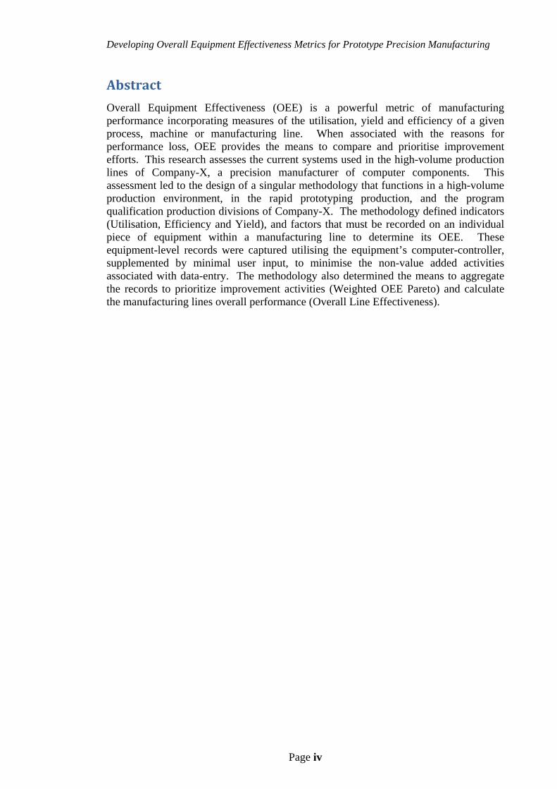
Abstract
Overall Equipment Effectiveness (OEE) is a powerful metric of manufacturing performance incorporating measures of the utilisation, yield and efficiency of a given process, machine or manufacturing line. When associated with the reasons for performance loss, OEE provides the means to compare and prioritise improvement efforts. This research assesses the current systems used in the high-volume production lines of Company-X, a precision manufacturer of computer components. This assessment led to the design of a singular methodology that functions in a high-volume production environment, in the rapid prototyping production, and the program qualification production divisions of Company-X. The methodology defined indicators (Utilisation, Efficiency and Yield), and factors that must be recorded on an individual piece of equipment within a manufacturing line to determine its OEE. These equipment-level records were captured utilising the equipment’s computer-controller, supplemented by minimal user input, to minimise the non-value added activities associated with data-entry. The methodology also determined the means to aggregate the records to prioritize improvement activities (Weighted OEE Pareto) and calculate the manufacturing lines overall performance (Overall Line Effectiveness).
Developing Overall Equipment Effectiveness Metrics for Prototype Precision Manufacturing
Page v
Contents1 Introduction ........................................................................................................................... 1
1.1 Background of Company-X ........................................................................................... 2
1.2 Genesis of the project at Company-X ............................................................................ 5
1.3 Research Methodology .................................................................................................. 6
1.4 Chapter Summary .......................................................................................................... 7
2 Literature Survey ................................................................................................................... 8
2.1 Overall Equipment Effectiveness .................................................................................. 8
2.2 Utilisation Indicator vs. Availability Efficiency .......................................................... 12
2.3 Efficiency Indicator vs. Performance Efficiency ......................................................... 15
2.4 Yield Indicator vs. Quality Efficiency ......................................................................... 17
2.5 Cause Data & Pareto Charts ........................................................................................ 20
2.6 Overall Effectiveness Line Metrics ............................................................................. 21
2.7 Data Collection and Cross Functional Teams .............................................................. 23
3 Development of Lean Data Collection ................................................................................ 26
3.1 Initial Data-collection practices ................................................................................... 26
3.2 Leaning the data-collection process ............................................................................. 29
3.3 Proposed data-collection process ................................................................................. 30
3.4 Chapter Summary ........................................................................................................ 31
4 Development of Utilisation Capture ................................................................................... 32
4.1 Time where the equipment is running ......................................................................... 32
4.2 Time where the equipment is idle ................................................................................ 35
4.3 Time where the equipment is unable to run due to some unscheduled event .............. 38
4.3.1 Equipment triggered unscheduled event ............................................................... 39
4.3.2 Operator triggered unscheduled event .................................................................. 40
4.4 Time where the equipment is not run due to some scheduled event ............................ 43
4.4.1 Switching Modes ................................................................................................... 43
4.4.2 Incentives to make the correct selection ............................................................... 45
4.4.3 Focused functionality ............................................................................................ 46
4.4.4 Visible current status ............................................................................................. 47
4.4.5 Activity goals ........................................................................................................ 50
4.5 Reliability ..................................................................................................................... 51
Developing Overall Equipment Effectiveness Metrics for Prototype Precision Manufacturing
Page vi
4.5.1 Restoration recording ............................................................................................ 52
4.5.2 Incremental recording ........................................................................................... 55
4.6 Final development at Company-X ............................................................................... 57
4.6.1 Removal of prompt when user pressed stop ......................................................... 59
4.6.2 Changes to Process Reaction Mode ...................................................................... 60
4.6.3 Removal of various entry fields on interface ........................................................ 61
4.7 Reconciling PTM, PDM & HVM utilisation indicators .............................................. 63
4.8 Chapter Summary ........................................................................................................ 64
5 Development of Efficiency & Yield Capture ...................................................................... 65
5.1 Efficiency Capture ....................................................................................................... 65
5.1.1 Rated Cycle-time and Output-rate ........................................................................ 65
5.1.2 Actual Cycle-time ................................................................................................. 66
5.1.3 Actual Output-rate ................................................................................................. 67
5.1.4 Proposed standard method for Actual values ........................................................ 68
5.2 Yield Capture ............................................................................................................... 68
5.2.1 Count of the number of units input to the equipment ........................................... 69
5.2.2 Count of the number of units output from the equipment ..................................... 72
5.2.3 Count of the number of defective units created by the equipment ........................ 74
5.2.4 Recommended Yield Capture System .................................................................. 76
5.2.5 Systems at Company-X & Equipment-Z .............................................................. 77
5.3 Chapter Summary ........................................................................................................ 79
6 Developing Pareto & Line Metrics ..................................................................................... 80
6.1 “Grand Pareto” & OEE Pareto ..................................................................................... 80
6.2 Line productivity as a function of equipment productivity .......................................... 83
6.2.1 Overall Line Effectiveness .................................................................................... 83
6.2.2 Utilisation .............................................................................................................. 84
6.2.3 Efficiency .............................................................................................................. 85
6.2.4 Yield ...................................................................................................................... 85
6.3 Chapter Summary ........................................................................................................ 86
7 Conclusions & Recommendations ...................................................................................... 87
7.1 Conclusions .................................................................................................................. 87
7.2 Recommendations ........................................................................................................ 88

Developing Overall Equipment Effectiveness Metrics for Prototype Precision Manufacturing
Page vii
8 References ........................................................................................................................... 89
Developing Overall Equipment Effectiveness Metrics for Prototype Precision Manufacturing
Page viii
ListofFigures
Figure 2-1 Graphical representation of OEE and Losses [10] .................................................... 10
Figure 2-2 Graph showing accumulative affects of loss on OEE ............................................... 11
Figure 2-3 Classification ambiguity in SEMI E79 [7] ................................................................ 14
Figure 2-4 Basic model of capturing yield indicator from its factors ......................................... 18
Figure 2-5 Model of capturing yield factors with pristine units ................................................. 19
Figure 2-6 Example of a Pareto Chart ........................................................................................ 20
Figure 3-1 Data capture process with muda ............................................................................... 27
Figure 3-2 Data capture process with indicated changes ............................................................ 30
Figure 3-3 Proposed, lean data capture process .......................................................................... 30
Figure 4-1 Process of capturing equipment time ........................................................................ 34
Figure 4-2 Equipment-Z's user interface showing Event Log .................................................... 41
Figure 4-3 Prompt to user to capture reason for stopping equipment ......................................... 42
Figure 4-4 Basic & Additional function of Equipment-Z's interface .......................................... 46
Figure 4-5 "Traffic-light" colour-coding of utilisation impact ................................................... 48
Figure 4-6 Colour-coding of equipment modes .......................................................................... 50
Figure 4-7 User prompt when exiting Equipment-Z's user interface .......................................... 52
Figure 4-8 User prompt when restarting Equipment-Z's user interface after abnormal exit ...... 54
Figure 4-9 User response time to utilisation-tracking interface .................................................. 58
Figure 4-10 Example of interface when responding to a feed-line jam ...................................... 62
Figure 4-11 Example of interface when responding to a process check failure ......................... 62
Figure 5-1 Yield tracking is complicated when accumulator are used ....................................... 69
Figure 5-2 Representation of carrier used to transport unit through the manufacturing line ...... 70
Figure 5-3 Yield tracking is complicated when carriers are used ............................................... 70
Figure 5-4 Yield tracking is complicated when units out is assumed ......................................... 72
Figure 5-5 Yield tracking model to address carriers and accumulators ...................................... 77
Figure 6-1 Pareto of utilisation loss ............................................................................................ 80
Figure 6-2 Pareto of efficiency loss ............................................................................................ 80
Figure 6-3 Pareto of yield loss .................................................................................................... 81
Figure 6-4 Pareto of all OEE loss ............................................................................................... 81
Figure 6-5 Pareto of weighted OEE loss ..................................................................................... 83

Developing Overall Equipment Effectiveness Metrics for Prototype Precision Manufacturing
Page ix
Figure 6-6 Line Yield treating all equipment as one large process ............................................ 86
Developing Overall Equipment Effectiveness Metrics for Prototype Precision Manufacturing
Page x
ListofTables
Table 2-1 Cumulative effects of loss on OEE ............................................................................ 10
Table 2-2 Usage of the OEE metric ............................................................................................ 12
Table 4-1 Basic structure of Equipment-Z’s event log ............................................................... 33
Table 4-2 Equipment-Z’s event log with utilisation events ........................................................ 35
Table 4-3 Example of reasons (cause) of idle events .................................................................. 37
Table 4-4 The various activities and modes that can occur on Equipment-Z ............................. 44
Table 4-5 Need for further categorisation modes that can occur on Equipment-Z ..................... 45
Table 4-6 The functionality of each mode programmed into Equipment Z ............................... 47
Table 4-7 Colour-coding of equipment modes ........................................................................... 49
Table 4-8 Example of reporting errors ........................................................................................ 56
Table 4-9 Example of solution to basic reporting errors ............................................................ 57
Table 4-10 Example of improved reporting with transformed data ............................................ 57
Table 4-11 Activity goals per phase of program life-cycle ........................................................ 64
Table 5-1 Breakdown of yield capture issues per Company-X’s equipment .............................. 78
Table 6-1 Top three losses from the previous Pareto charts ....................................................... 83
Developing Overall Equipment Effectiveness Metrics for Prototype Precision Manufacturing
Page 1 Michael O’Neill
1 Introduction
Overall Equipment Effectiveness, or OEE for short, is a productivity and performance
metric that is widely discussed in the manufacturing industry. While the theoretical
merits of the metrics are understood and accepted, the application is a challenge to any
manufacturing organisation.
One challenge of OEE is the adaptation of a metric primarily used for capacity planning
and improvement of high-volume manufacturing performance to a manufacturing
environment that performs low-volume prototype builds mixed with extensive
product/process development and testing. How can a single system for tracking OEE be
deployed in an environment that facilitates prototype manufacturing, product/process
development and high-volume manufacturing?
This was the challenge facing Company-X. Despite various systems deployed to track
the OEE of its high-volume manufacturing lines, these same systems proved to be
confusing and were ultimately rejected when deployed on the prototyping and
development lines.
Unless a single system can be designed and developed to track the OEE of all
equipment and manufacturing lines regardless of the focus (prototype; development;
volume of lines) it cannot be installed and used to improve performance of the overall
manufacturing system utilised by the company. This is due to:
1. Company-X personnel whom support prototype, development and high-volume
lines will not easily accept three different systems and metrics
2. Company-X will not have a metric that predicts how well a prototype or
development product will perform at development or high-volume respectively.
3. Company-X will not be able to create performance goals or baselines for
prototype or development line’s performance that correlated to high-volume
performance.
Developing Overall Equipment Effectiveness Metrics for Prototype Precision Manufacturing
Page 2 Michael O’Neill
1.1 BackgroundofCompany‐X
Company-X is a precision manufacturing company which specializes in components for
the hard-drive industry. The company has a practice of developing new iterations of the
same or similar products for its customers to win contracts for new programs (future
products or product lines). This development process results in the program life-cycle
having three phases:
Prototype Manufacturing (PTM)
Program-development Manufacturing (PDM)
High-volume Manufacturing (HVM)
The first is initial prototyping where units (individual pieces of product) are fabricated
on stand-alone equipment and standard tooling in batch volume. These units are used
by the customer to evaluate the viability of the components in their assemblies. In this
phase, the goal of Company-X is to have the shortest lead time from placing a build
order to shipping the product. These prototyping build occur at the Company-X’s
prototype manufacturing (PTM) lines.
Based on this evaluation, the customer will request units, but with an eye to sourcing a
high-volume supplier. At this point, Company-X will move from the stand-alone
equipment to a coupled line with dedicated tooling which are optimized to meet the
product specifications. Low volume manufacturing orders of these units are purchased
by the customer to develop and qualify a particular hard-drive design. The goal for
Company-X is to provide these units on time, at superior quality and at a lower cost
compared to Company-X’s competitors who are also trying to qualify their design with
the customer. This allows the customer to see Company-X as a viable supplier for the
program as well as qualify Company-X and the product design for high volume
production. These activities occur on Company-X’s program-development
manufacturing (PDM) lines.
Upon being qualified as a high-volume supplier, Company-X will establish one or more
high-volume manufacturing (HVM) lines to meet the demands of the customer. More
often than not this warrants high-volume 24/7 production. Company-X specifically
“pulses” the PTM line to evaluate the line’s throughput and yield. “Pulsing” is the
practice of running the manufacturing-line at maximum capacity and taking the quickest
action to restart and stoppages without investigating or resolving root-cause during the
Developing Overall Equipment Effectiveness Metrics for Prototype Precision Manufacturing
Page 3 Michael O’Neill
build. The pulse is to simulate the line under HVM conditions. Staff would also
diligently record the condition which caused the stoppage and any yield loss. The
transfer of tooling and equipment from the PDM-focused line to one of the HVM-
focused lines was contingent on passing a set of criteria which indicated the line’s
reliability in producing units at a rate and quality to maintain good profit margins.
Should these criteria not be met, engineering would address the issues recorded during
the pulse and correct them before the next pulse.
Due to increased and evolving market pressures, the opportunity to prove the line’s
reliability and to progressively ramp-up to high-volume have been diminished.
Customers’ expect a qualified program to immediately yield between 50% and 75%
units per week per line compared to full high-volume capacity. This market pressure
decreased the pulsing and reliability testing activities as Company-X’s focus has been
on keeping the customer satisfied by meeting the volume rates and commit dates.
Failure to meet the volume rates and commitment dates can lead to Company-X not
being the preferred supplier on this or future programs.
Engineers within Company-X know and understand Overall Equipment Effectiveness
(OEE) as the most reliable measure of equipment productivity. Unfortunately, the
company’s primary focus is on “Delivery to Commit” and “Customer Incident
Reduction”. “Delivery to Commit” means ensuring that all manufacturing orders are
filled regardless of yield rates manual sorting and over-time. “Customer Incident
Reduction” means ensuring the customer does not detect and report an issue with the
quality of the shipped units.
The problem with these metrics is that they are captured and recorded at the end of the
manufacturing process. While a drop in these metrics will indicate a significant error
that the company should respond to, the damage will already have been done with
respect to the customer. Their ordered shipment will either be recommitted, with a
future ship date determined, cancelled, or contain less than perfect or unacceptable
product. None of these outcomes is favourable to the company’s long-term relationship
with the customer.
Understanding this, the industrial and manufacturing engineers at the company have
worked piece-meal over time to establish more predictive metrics. They have
established defect tracking systems and down-time tracking systems. In addition, they
have established a means of calculating the OEE for each manufacturing line.
Developing Overall Equipment Effectiveness Metrics for Prototype Precision Manufacturing
Page 4 Michael O’Neill
To date, the culture at Company-X has not embraced the OEE metric and therefore
management has established neither baselines nor goals. There are two keys reasons for
this, each of which will be examined in this thesis:
1. Lack of confidence in the accuracy of the metric
2. Lack of use of these metrics in the PTM & PDM phases
The existing methods are not flawless and their shortcomings can quickly be seen by
anyone required to interact with these systems: those responsible for capturing the data
and those using it. This lack of confidence has a ‘downward-spiral’ effect. With the
quality of the metric data output in question, it does not get used. When those at the
front-end of the system know that those at the back-end of the system are not using the
data, the care and effort they invest the system degrades. This degradation further
impacts the quality of the output metrics and the cycle starts over again.
Specifically in the PDM plant, these metrics are viewed as only being important for
those programs at the HVM plants. In PDM, builds are low and changes are plentiful.
In HVM, volumes are high and the program is qualified and therefore not subject to
frequent change. The perception is that it is easier and more valuable to capture,
develop trends and address issues with yield, down-time and cycle-time in the HVM
line as it is more “stable”. While a “stable” system is undoubtedly easier to characterise
than an “unstable” system there is a significant reason as to why this perception exists at
Company-X.
To a certain degree, Company-X treats every program as if it was a brand-new product
that was not previously manufactured when in reality most programs are following on
from previous programs, e.g. the customer used to retail a 10 GB laptop drive and is
phasing out that product for a 50 GB drive. Many of the product’s design requirements
and components are the same or have some minor evolution. The point being that
understanding the manufacturing productivity of the 10 GB program will result in a
reasonable baseline of the productivity the 50 GB should achieve.
This understanding needs to be developed for each of the three stages of the lifetime of
the program: the concept prototyping (PTM), the low-volume supplier qualification
(PDM), and the high-volume manufacturing (HVM). A baseline of all three phases will
serve as a means to monitor the new program at all phases. Similarly, understanding the
Developing Overall Equipment Effectiveness Metrics for Prototype Precision Manufacturing
Page 5 Michael O’Neill
relationship between PTM productivity and the later phases will serve as a predictor of
future problems and opportunities before the program does mature to the later phases.
Company-X’s existing systems were developed for the HVM plants and then later
deployed to the PTM & PDM plant. One key flaw to this is the reliance of the systems
to exist in a manufacturing line of continuous, coupled equipment. PTM lines have
decoupled equipment and require more manual operation (e.g. the loading and
unloading of units to and from equipment) from the personnel. Lack of the systems
available in coupled lines resulted in only throughput quantities being manually tracked
on PTM to ensure the ordered quantity was achieved.
A compounding issue is that there was no specific focus on making the systems lean;
lean referring to the principles of Lean Manufacturing[1]. For example, let us assume
the yield-tracking system takes 5 minutes of user-time to classify and log a detected
defect on a unit. As the productivity of the program should improve over the program
lifecycle, the occurrence of these defects should be rare enough that the 5 minutes is a
negligible impact on productivity by the time it reaches the HVM phase. In the PTM
phase where defects and down-time events are expected and numerous, 5 minutes per
occurrence is too significant of an impact to productivity to be ignored. The lack of an
efficient system means the volume of work to capture this data is high and therefore not
available in an environment where lead-time for shipping is critical.
1.2 GenesisoftheprojectatCompany‐X
Company-X’s systems are not uniform amongst all the equipment and plants, indeed
within a single line there are three different methods of recording defects. While this
lack of uniformity needs to be progressively removed, it provides the opportunity to
compare and contrast the different methods and propose the best alternative.
Additionally, the issues with these systems are well documented and understood.
These issues were not previously resolved due lack of a department with the resources
and remit to prioritise and address them. Engineering groups either had a customer
(product specific) focus or an equipment specific focus. The creation of an engineering
role responsible for improving the transition of a program through the three phases
became the genesis of an effort to define metrics for determining the productivity of the
manufacturing. The department was named ‘Operations Manufacturing Engineering’ or
OME for short.
Developing Overall Equipment Effectiveness Metrics for Prototype Precision Manufacturing
Page 6 Michael O’Neill
The author was hired by Company-X as an Operations Manufacturing Engineer to find
that no metrics and baseline existed to correlate performance of a PTM or PDM line
with a HVM line. The first action of the author in this role was to develop these
metrics. The author proposed the development of lean systems that would capture data
needed to compile OEE for each individual piece of equipment. These systems would:
Function in the PTM environment
Function in the PDM environment
Function in the HVM environment
Be accepted and properly used by all personnel due to their ease of use
Be accepted as an accurate productivity metric by management
Allow for baselines to be created and OEE goals to be set
Provide a threshold to trigger preventative and proactive measures to ensure
delivery dates and customer satisfaction
Allow the data from all manufacturing builds to be collected
Eliminate the need for pulsing by providing pulse-like data for every
manufacturing order
It was determined that Equipment-Z, which performs several critical value-added
operations, would be used to develop the proposed OEE system. It would serve as the
proof-of-concept and ultimately would be used to justify work to expand the system to
all of Company-X’s equipment.
1.3 ResearchMethodology
As the Operations Manufacturing Engineer for Equipment-Z, this work was undertaken
by the author and is represented in this thesis. While the input and approval of many
individuals was required for the testing and refinement of this system, the author
performed as system designer and software programmer. The system was then
developed, tested and improved in the following manner:
1. Investigate existing methods, both internal to Company-X and in the broader
industry, and in academic papers.
Developing Overall Equipment Effectiveness Metrics for Prototype Precision Manufacturing
Page 7 Michael O’Neill
2. Devise new approach, one that break the Information Paradox as much as
possible, and an implementation plan.
3. Review new approach and implementation direct end-users and technical
support of end-users before developing code
4. Develop code and implement pilot on specific instances of Equipment-Z for a
define period of time.
5. Review and evaluate approach and code the same personnel in step 3:
a. Make revisions as necessary and repeat steps 3 to 5.
b. Once final version was agreed upon, proceed to step 6.
6. Review and evaluate performance with Management & Engineering; once
approved, changes would be implemented in all instances of Equipment-Z, and
plans to develop and implement for all other devices would be executed.
1.4 ChapterSummary
This project will develop a new singular, OEE metric implementation suitable for
prototype, program-development and high-volume manufacturing lines.
Developing Overall Equipment Effectiveness Metrics for Prototype Precision Manufacturing
Page 8 Michael O’Neill
2 LiteratureSurvey
If a goal is to be achieved it must be measurable. This is particularly true in
manufacturing where profit is dependant on the productivity of its people and
equipment [2]. As de Ron and Rooda state [3]:
[H]undreds of performance measures are being used. Managers want to have one
clear metric and dislike the plurality of information.
As no one traditional metric, such as yield or utilisation, depicts the whole picture.
Worse still is improvement on one metric can come at the cost of another [4]. Some
aggregate of existing measures is needed. From here forward the term metric will be
reserved for the aggregated measure while indicator will be used for the measures that
comprise this metric. It is important that these measures be accurately and reliably
captured to ensure any completed activities will lead to improved productivity [5].
2.1 OverallEquipmentEffectiveness
There are many potential goals and indicators that can be used. Poorly set goals will
lead to inter-departmental conflict [6]. Three commonly used for manufacturing
performance [5] & [7]:
Availability or Availability Efficiency
Performance Rate or Performance Efficiency
Quality Rate or Quality Efficiency
While these naming conventions were codified by SEMI, companies such as Company-
X often refers to the indicators respectively as:
Utilisation, U – the usage rate of the equipment, the ratio of actual running of
the equipment versus availability of the equipment
Efficiency, E – the output-rate of the equipment, the ratio of actual speed
versus the rated speed of the equipment
Yield, Y – the quality rate of the equipment, the ratio of good units output
versus of total units input to the equipment
Any differences between SEMI and Company-X will be explained later in this report.

Developing Overall Equipment Effectiveness Metrics for Prototype Precision Manufacturing
Page 9 Michael O’Neill
A common practice in productivity improvement activities is to:
1. Calculate the indicator, e.g. utilisation of all the equipment in a line
2. Identify which equipment has the lowest indicator value
3. Create a Pareto chart of the reasons for loss on that equipment
4. Focus on reducing or eliminating the top contributors as indicated by the Pareto
chart
The problem of using these indicators in isolation is that none convey the actual
productivity of the equipment. Consider productivity in terms of units produced within
a fixed time frame:
If the equipment is not available for use, e.g. it breaks down, there will less
processing time (hours) and therefore fewer units are produced
If the equipment runs slower than its top speeds, its output-rate (units per hour)
is decreased and therefore fewer units are produced
If the equipment produces more defects, e.g. a shear die becomes dull, the
fewer acceptable units are produced
A singular measure is required to reveal the all the productivity loss. Such losses
constitute lost opportunity and non-value-added costs. These costs are of significant
importance to any manufacturer; hidden costs in particular [8] & [9]. If a manufacturer
assumes only loss of processing time as productivity loss, the cost of slow equipment
will be hidden to them.
Utilisation, Efficiency and Yield each contribute to the ease of an equipment to produce
quality units in a timely manner. As each of these indicators are a ratio (or percentage)
whereby 1 (or 100%) represents the perfect state of the equipment, these indicators can
be combined via multiplication of these indicators. This combination is a metric called
Overall Equipment Effectiveness or OEE can be seen in Equation 1.
Developing Overall Equipment Effectiveness Metrics for Prototype Precision Manufacturing
Page 10 Michael O’Neill
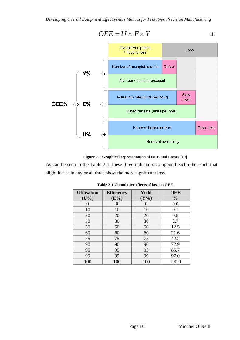
YEUOEE (1)
Figure 2-1 Graphical representation of OEE and Losses [10]
As can be seen in the Table 2-1, these three indicators compound each other such that
slight losses in any or all three show the more significant loss.
Table 2-1 Cumulative effects of loss on OEE
Utilisation (U%)
Efficiency (E%)
Yield (Y%)
OEE %
0 0 0 0.0 10 10 10 0.1 20 20 20 0.8 30 30 30 2.7 50 50 50 12.5 60 60 60 21.6 75 75 75 42.2 90 90 90 72.9 95 95 95 85.7 99 99 99 97.0 100 100 100 100.0
Developing Overall Equipment Effectiveness Metrics for Prototype Precision Manufacturing
Page 11 Michael O’Neill
0%
20%
40%
60%
80%
100%
0% 20% 40% 60% 80% 100%
U%, E%
and Y%
OEE = U% x E% x Y%
Overall Equipment Effectiveness
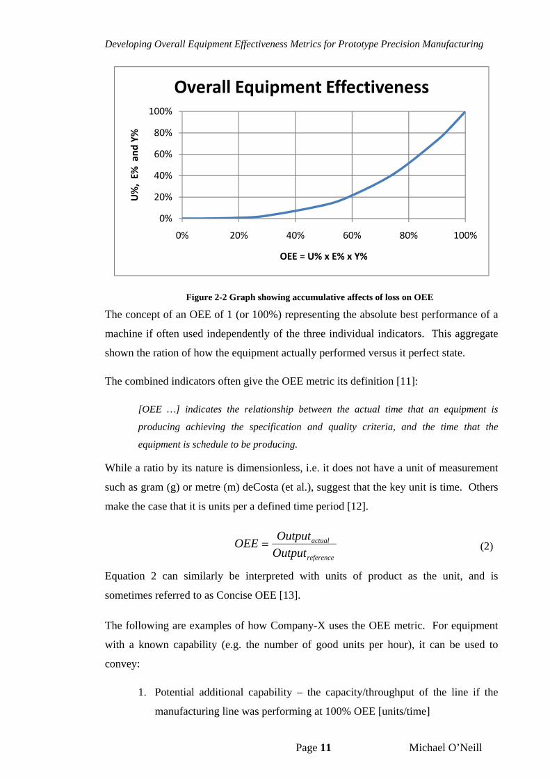
Figure 2-2 Graph showing accumulative affects of loss on OEE
The concept of an OEE of 1 (or 100%) representing the absolute best performance of a
machine if often used independently of the three individual indicators. This aggregate
shown the ration of how the equipment actually performed versus it perfect state.
The combined indicators often give the OEE metric its definition [11]:
[OEE …] indicates the relationship between the actual time that an equipment is
producing achieving the specification and quality criteria, and the time that the
equipment is schedule to be producing.
While a ratio by its nature is dimensionless, i.e. it does not have a unit of measurement
such as gram (g) or metre (m) deCosta (et al.), suggest that the key unit is time. Others
make the case that it is units per a defined time period [12].
reference
actual
Output
OutputOEE
(2)
Equation 2 can similarly be interpreted with units of product as the unit, and is
sometimes referred to as Concise OEE [13].
The following are examples of how Company-X uses the OEE metric. For equipment
with a known capability (e.g. the number of good units per hour), it can be used to
convey:
1. Potential additional capability – the capacity/throughput of the line if the
manufacturing line was performing at 100% OEE [units/time]
Developing Overall Equipment Effectiveness Metrics for Prototype Precision Manufacturing
Page 12 Michael O’Neill
2. Potential reduction in manufacturing time per manufacturing order – if line
was performing at 100% OEE [time]
3. The number of units-worth of raw material that needs to be input to the
manufacturing line to produce the desired number of acceptable units (due to
yield loss) – based on current OEE [units]
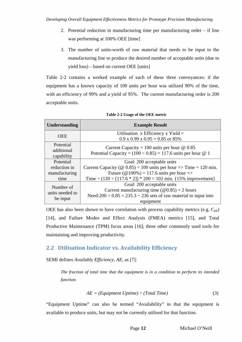
Table 2-2 contains a worked example of each of these three conveyances: if the
equipment has a known capacity of 100 units per hour was utilized 90% of the time,
with an efficiency of 99% and a yield of 95%. The current manufacturing order is 200
acceptable units.
Table 2-2 Usage of the OEE metric
Understanding Example Result
OEE Utilisation x Efficiency x Yield = 0.9 x 0.99 x 0.95 = 0.85 or 85%
Potential additional capability
Current Capacity = 100 units per hour @ 0.85 Potential Capacity = (100 ÷ 0.85) = 117.6 units per hour @ 1
Potential reduction in
manufacturing time
Goal: 200 acceptable units Current Capacity (@ 0.85) = 100 units per hour => Time = 120 min.
Future (@100%) = 117.6 units per hour => Time = (120 ÷ [117.6 * 2]) * 200 = 102 min. {15% improvement}
Number of units needed to
be input
Goal: 200 acceptable units Current manufacturing time (@0.85) = 2 hours
Need:200 ÷ 0.85 = 235.3 ~ 236 sets of raw material to input into equipment
OEE has also been shown to have correlation with process capability metrics (e.g. Cpk)
[14], and Failure Modes and Effect Analysis (FMEA) metrics [15], and Total
Productive Maintenance (TPM) focus areas [16]; three other commonly used tools for
maintaining and improving productivity.
2.2 UtilisationIndicatorvs.AvailabilityEfficiency
SEMI defines Availably Efficiency, AE, as [7]:
The fraction of total time that the equipment is in a condition to perform its intended
function.
AE = (Equipment Uptime) ÷ (Total Time) (3)
“Equipment Uptime” can also be termed “Availability” in that the equipment is
available to produce units, but may not be currently utilised for that function.
Developing Overall Equipment Effectiveness Metrics for Prototype Precision Manufacturing
Page 13 Michael O’Neill
As understood in Company-X, Utilisation, U, is the ratio of time the equipment spent
running i.e. producing product versus the total Available-Time:
Avail
Run
T
TU (4)
There is a distinctive difference between SEMI’s standard and Company-X’s definition.
Uptime includes more than just running-time in that it is potential running time and not
actual running-time. This means it that Availability Efficiency does not include minor
stoppages and idle-time events due to operational losses. These losses are captured in
the Operational Efficiency component of the Performance Efficiency indicator. This
makes Operation Efficiency or Utilisation more difficult to document as unlike
Availability Efficiency it requires capture and quantification of unplanned events [17].
Another difference in is that SEMI allows for “Engineering Time” to be included in
“Equipment Uptime”. Staff in Company-X different lines would argue if it similarly be
counted with pure production time as TRun. Other companies question similarly question
if such non-productive activities can be considered as Down-Time even if the
equipment is operable as these are activities that they would aspire to minimise [17].
Available time is typically the total calendar hours within a period of time less the hours
of Scheduled-Down-Time.
SchdCalendar
Run
Avail
RunTT
T
T
TU
(5)
Scheduled-Down-Time events can include:
Preventative Maintenance
Retooling for next build
Engineering testing.
If Running-Time is not explicitly measured, it is calculated by measuring the non-
Running-Time and removing that from the calendar time. This non-Running-Time, or
Down-Time, in turn is broken down into Scheduled-Down-Time, Unscheduled-Down-
Time and Idle-Time. Idle-Time reflects the time the equipment was operational but was
unable to process product. A common example of an idle condition is the equipment
not have units feed into it, or the equipment is unable to index to the next unit as the line
has stopped downstream.
Developing Overall Equipment Effectiveness Metrics for Prototype Precision Manufacturing
Page 14 Michael O’Neill
SchdCalendar
IdleUnschdSchdCalendar
Avail
RunTT
TTTT
T
TU
(6)
If all machine time: Running-Time, Scheduled-Down-Time, Unscheduled-Down-Time
and Idle-Time is explicitly captured, the total calendar time should equal the summation
of all calculated time.
IdleUnschdSchdRunTotalCalendar TTTTTT (7)
SchdTotalSchdCalendarAvail TTTTT (8)
SchdTotal
Run
Avail
Run
TT
T
T
TU
(9)
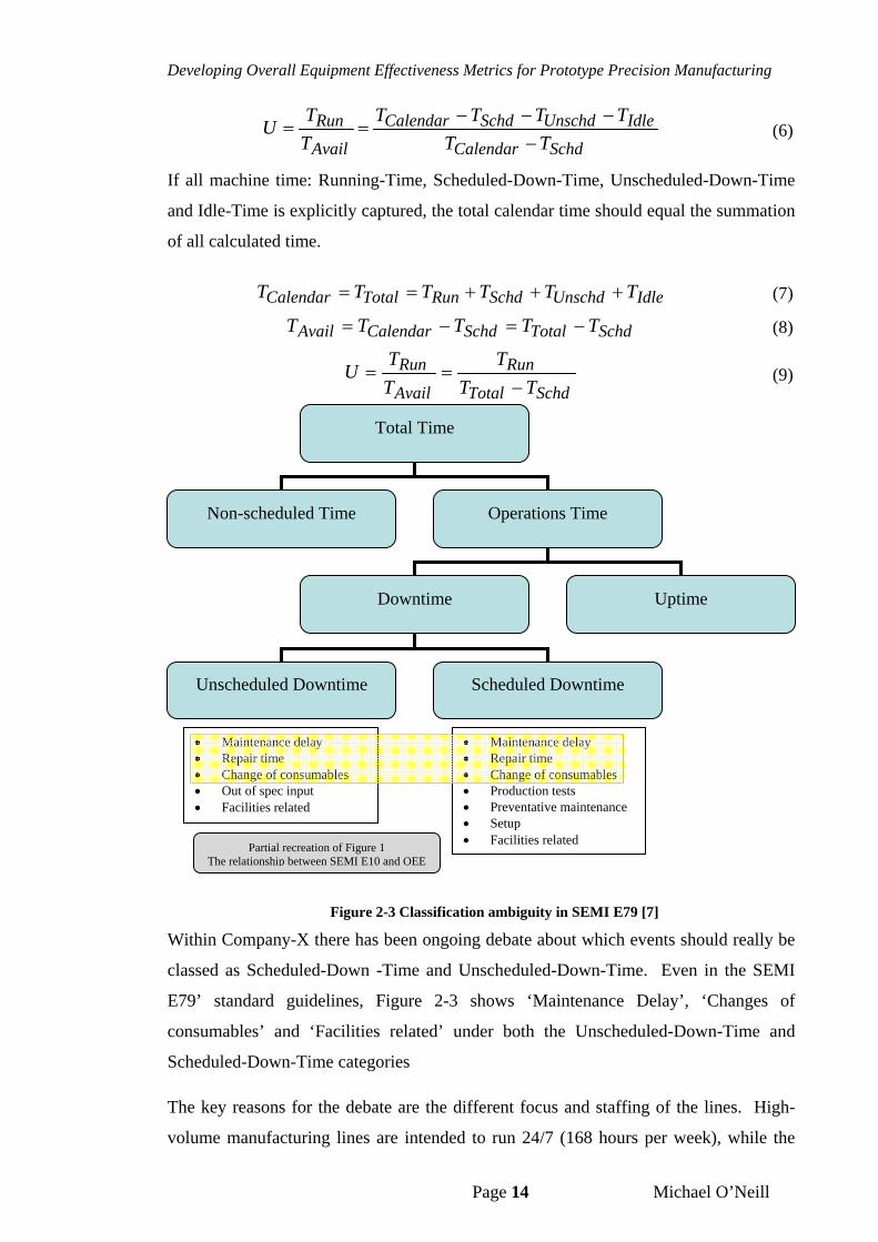
Figure 2-3 Classification ambiguity in SEMI E79 [7]
Within Company-X there has been ongoing debate about which events should really be
classed as Scheduled-Down -Time and Unscheduled-Down-Time. Even in the SEMI
E79’ standard guidelines, Figure 2-3 shows ‘Maintenance Delay’, ‘Changes of
consumables’ and ‘Facilities related’ under both the Unscheduled-Down-Time and
Scheduled-Down-Time categories
The key reasons for the debate are the different focus and staffing of the lines. High-
volume manufacturing lines are intended to run 24/7 (168 hours per week), while the
Total Time
Non-scheduled Time Operations Time
Downtime Uptime
Unscheduled Downtime Scheduled Downtime
Maintenance delay Repair time Change of consumables Production tests Preventative maintenance Setup Facilities related
Maintenance delay Repair time Change of consumables Out of spec input Facilities related
Partial recreation of Figure 1 The relationship between SEMI E10 and OEE
Developing Overall Equipment Effectiveness Metrics for Prototype Precision Manufacturing
Page 15 Michael O’Neill
PTM and PDM lines are intended to run 24/5 (120 hours per week) assuming no
overtime. There are those who contend that all lines should be measured equally, but in
the HVM plant there are rarely product changeovers due to product-dedicated lines, no
engineering testing and no room for overtime.
The simplest solution is to agree to use the straight dictionary definition of scheduled
and unscheduled. The PTM environment, however, lends itself to confusion as debug-
time is inherent and difficult to quantify beforehand to pragmatically schedule it.
Therefore within Company-X, business rules had to be established to consistently
communicate uptime/downtime, scheduled/unscheduled status of the equipment.
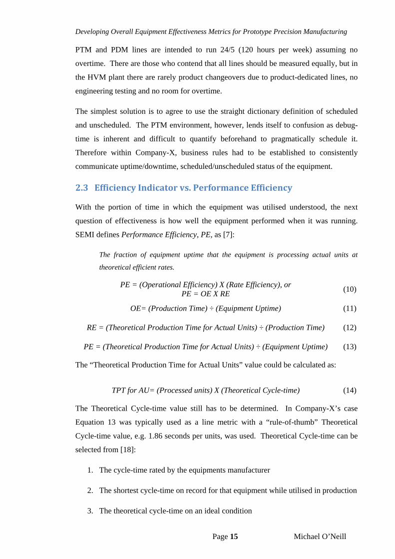
2.3 EfficiencyIndicatorvs.PerformanceEfficiency
With the portion of time in which the equipment was utilised understood, the next
question of effectiveness is how well the equipment performed when it was running.
SEMI defines Performance Efficiency, PE, as [7]:
The fraction of equipment uptime that the equipment is processing actual units at
theoretical efficient rates.
PE = (Operational Efficiency) X (Rate Efficiency), or PE = OE X RE
(10)
OE= (Production Time) ÷ (Equipment Uptime) (11)
RE = (Theoretical Production Time for Actual Units) ÷ (Production Time) (12)
PE = (Theoretical Production Time for Actual Units) ÷ (Equipment Uptime) (13)
The “Theoretical Production Time for Actual Units” value could be calculated as:
TPT for AU= (Processed units) X (Theoretical Cycle-time) (14)
The Theoretical Cycle-time value still has to be determined. In Company-X’s case
Equation 13 was typically used as a line metric with a “rule-of-thumb” Theoretical
Cycle-time value, e.g. 1.86 seconds per units, was used. Theoretical Cycle-time can be
selected from [18]:
1. The cycle-time rated by the equipments manufacturer
2. The shortest cycle-time on record for that equipment while utilised in production
3. The theoretical cycle-time on an ideal condition
Developing Overall Equipment Effectiveness Metrics for Prototype Precision Manufacturing
Page 16 Michael O’Neill
The third option is not expanded upon. Rather than speculate, the first two options
show a lot of room for ambiguity. The first is a measure of pure equipment speed; the
second can include dependencies on loading and unloading of units to and from the
equipment.
Company-X did not have a true equipment-level Performance Efficiency indicator.
Their utilisation indicator already absorbed some of the Operation Efficiency portion of
the Performance Efficiency. This is because Running-Time excludes the difference
between “Equipment Uptime” and “Production Time”. What remains to be accounted
for is purely Rate Efficiency, which Company-X simply referred to as Efficiency.
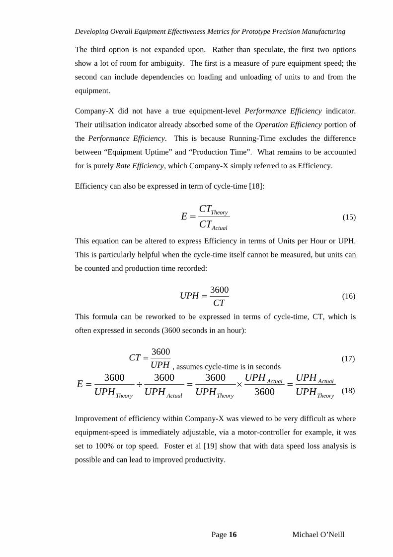
Efficiency can also be expressed in term of cycle-time [18]:
Actual
Theory
CT
CTE
(15)
This equation can be altered to express Efficiency in terms of Units per Hour or UPH.
This is particularly helpful when the cycle-time itself cannot be measured, but units can
be counted and production time recorded:
CTUPH
3600 (16)
This formula can be reworked to be expressed in terms of cycle-time, CT, which is
often expressed in seconds (3600 seconds in an hour):
UPHCT
3600
, assumes cycle-time is in seconds (17)
Theory
ActualActual
TheoryActualTheory UPH
UPHUPH
UPHUPHUPHE
3600
360036003600
(18)
Improvement of efficiency within Company-X was viewed to be very difficult as where
equipment-speed is immediately adjustable, via a motor-controller for example, it was
set to 100% or top speed. Foster et al [19] show that with data speed loss analysis is
possible and can lead to improved productivity.
Developing Overall Equipment Effectiveness Metrics for Prototype Precision Manufacturing
Page 17 Michael O’Neill
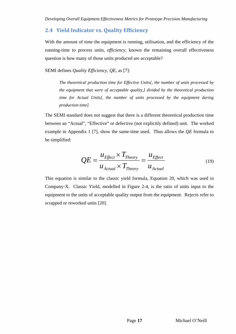
2.4 YieldIndicatorvs.QualityEfficiency
With the amount of time the equipment is running, utilisation, and the efficiency of the
running-time to process units, efficiency, known the remaining overall effectiveness
question is how many of those units produced are acceptable?
SEMI defines Quality Efficiency, QE, as [7]:
The theoretical production time for Effective Units[, the number of units processed by
the equipment that were of acceptable quality,] divided by the theoretical production
time for Actual Units[, the number of units processed by the equipment during
production time].
The SEMI standard does not suggest that there is a different theoretical production time
between an “Actual”, “Effective” or defective (not explicitly defined) unit. The worked
example in Appendix 1 [7], show the same-time used. Thus allows the QE formula to
be simplified:
Actual
Effect
TheoryActual
TheoryEffect
u
u
Tu
TuQE
(19)
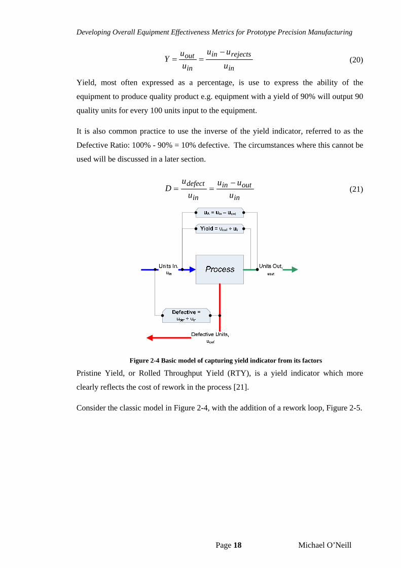
This equation is similar to the classic yield formula, Equation 20, which was used in
Company-X. Classic Yield, modelled in Figure 2-4, is the ratio of units input to the
equipment to the units of acceptable quality output from the equipment. Rejects refer to
scrapped or reworked units [20].
Developing Overall Equipment Effectiveness Metrics for Prototype Precision Manufacturing
Page 18 Michael O’Neill
in
rejectsin
in
outu
uu
u
uY
(20)
Yield, most often expressed as a percentage, is use to express the ability of the
equipment to produce quality product e.g. equipment with a yield of 90% will output 90
quality units for every 100 units input to the equipment.
It is also common practice to use the inverse of the yield indicator, referred to as the
Defective Ratio: 100% - 90% = 10% defective. The circumstances where this cannot be
used will be discussed in a later section.
in
outin
in
defect
u
uu
u
uD
(21)
Figure 2-4 Basic model of capturing yield indicator from its factors
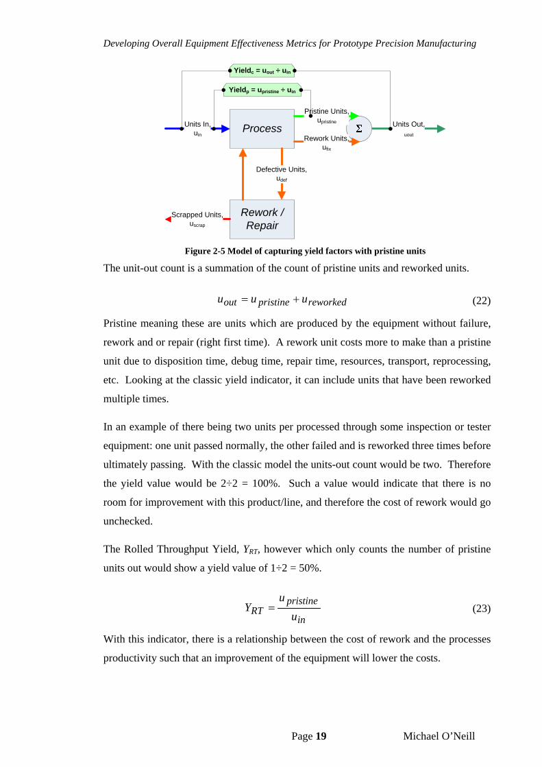
Pristine Yield, or Rolled Throughput Yield (RTY), is a yield indicator which more
clearly reflects the cost of rework in the process [21].
Consider the classic model in Figure 2-4, with the addition of a rework loop, Figure 2-5.
Developing Overall Equipment Effectiveness Metrics for Prototype Precision Manufacturing
Page 19 Michael O’Neill
Units Out,uout
Process
Pristine Units,upristine
Defective Units,udef
Rework / Repair
Scrapped Units,uscrap
Rework Units,ufix
Units In,uin
Yieldc = uout ÷ uin
Yieldp = upristine ÷ uin
Figure 2-5 Model of capturing yield factors with pristine units
The unit-out count is a summation of the count of pristine units and reworked units.
reworkedpristineout uuu (22)
Pristine meaning these are units which are produced by the equipment without failure,
rework and or repair (right first time). A rework unit costs more to make than a pristine
unit due to disposition time, debug time, repair time, resources, transport, reprocessing,
etc. Looking at the classic yield indicator, it can include units that have been reworked
multiple times.
In an example of there being two units per processed through some inspection or tester
equipment: one unit passed normally, the other failed and is reworked three times before
ultimately passing. With the classic model the units-out count would be two. Therefore
the yield value would be 2÷2 = 100%. Such a value would indicate that there is no
room for improvement with this product/line, and therefore the cost of rework would go
unchecked.
The Rolled Throughput Yield, YRT, however which only counts the number of pristine
units out would show a yield value of 1÷2 = 50%.
in
pristineRT u
uY (23)
With this indicator, there is a relationship between the cost of rework and the processes
productivity such that an improvement of the equipment will lower the costs.
Developing Overall Equipment Effectiveness Metrics for Prototype Precision Manufacturing
Page 20 Michael O’Neill
2.5 CauseData&ParetoCharts
Metrics and indicators are a necessary and powerful tool to track productivity, identify
trends and present opportunities for improvement. Indicators will not provide enough
information to capitalize on these opportunities [22]. It is not enough to know what
your OEE is. It must be coupled with the information that indicates why the metric is as
low (or high) as it is [3]. Indeed lack of this information is why establishment of OEE
has proven difficult for many companies [23], [24].
For example, a yield indicator is only effective if the type and source of the defects are
also known. From here forward in the report, the complementary data the provided
context to performance indicators is referred to a cause data. This cause data can be
used to determine trends and root-causes, and implement improvements internally
within the company and external with equipment suppliers [25].
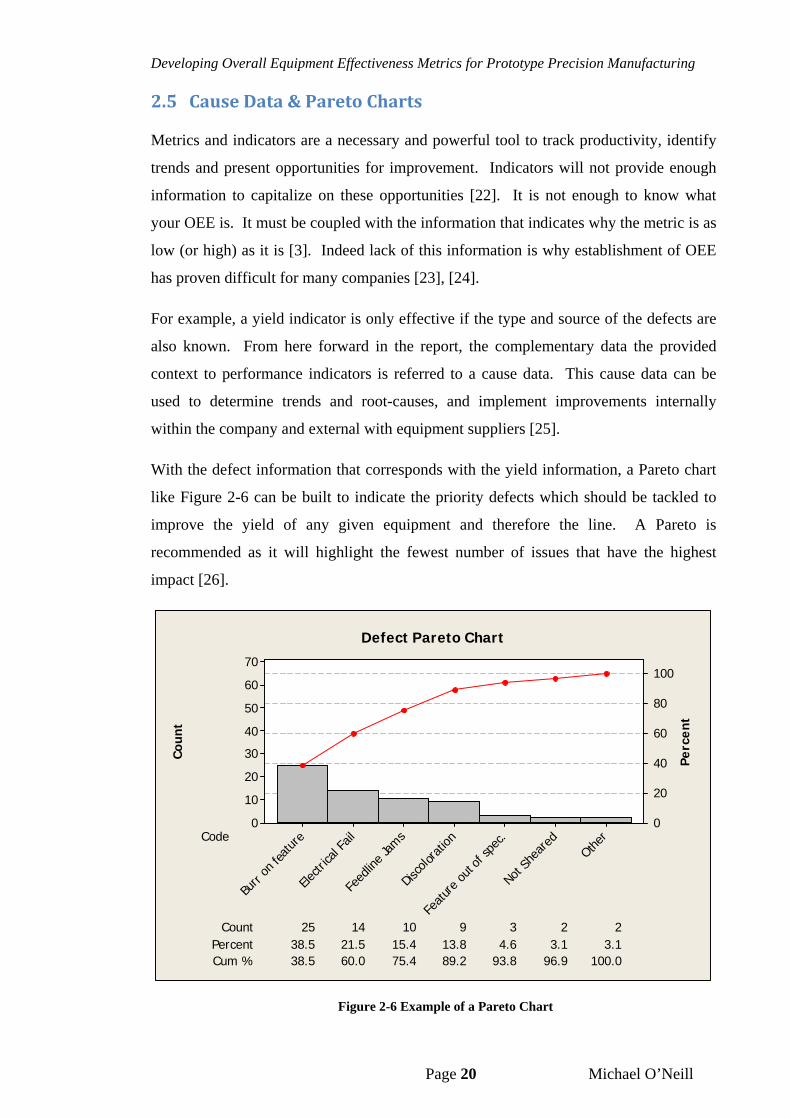
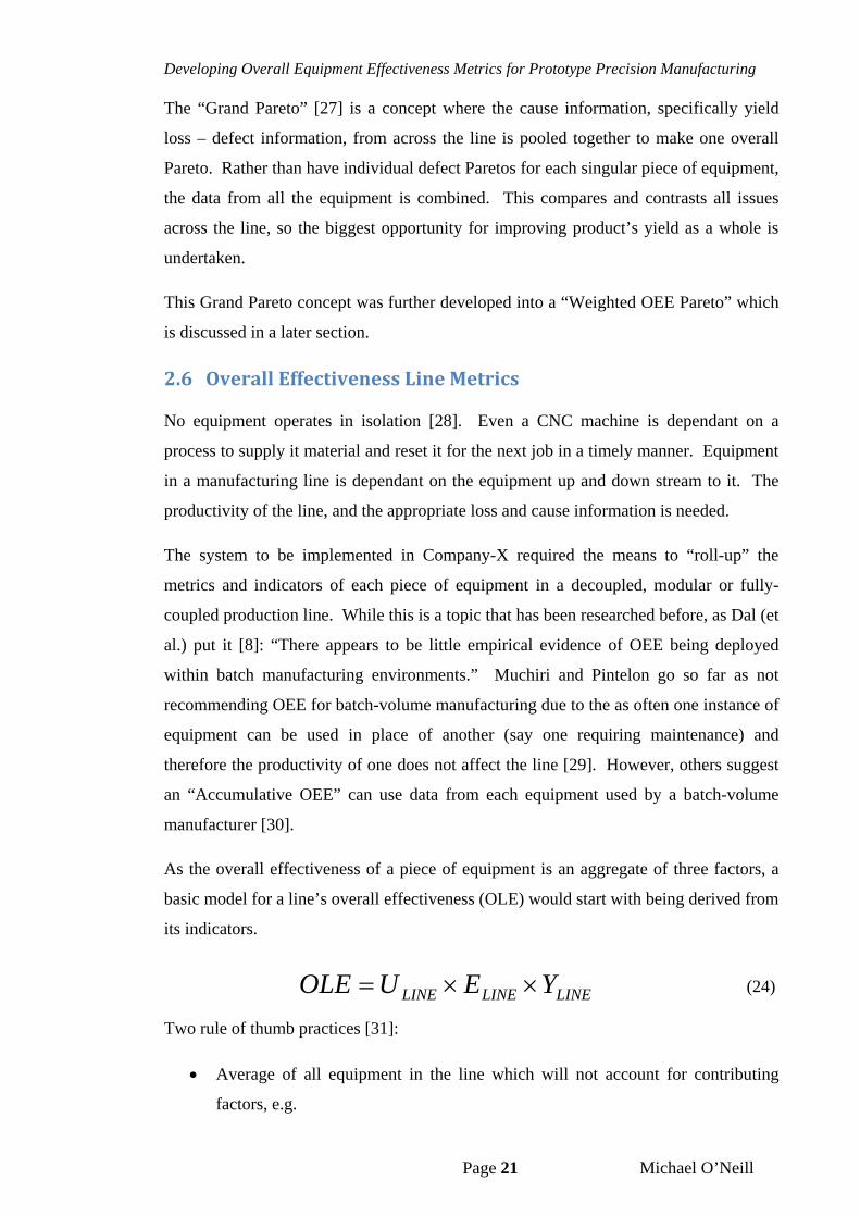
With the defect information that corresponds with the yield information, a Pareto chart
like Figure 2-6 can be built to indicate the priority defects which should be tackled to
improve the yield of any given equipment and therefore the line. A Pareto is
recommended as it will highlight the fewest number of issues that have the highest
impact [26].
Count 25 14 10 9 3 2 2Percent 38.5 21.5 15.4 13.8 4.6 3.1 3.1Cum % 38.5 60.0 75.4 89.2 93.8 96.9 100.0
CodeOthe
r
Not S
heare
d
Featu
re ou
t of s
pec.
Disco
lorati
on
Feed
line J
ams
Electr
ical F
ail
Burr
on fe
ature
70
60
50
40
30
20
10
0
100
80
60
40
20
0
Coun
t
Perc
ent
Defect Pareto Chart
Figure 2-6 Example of a Pareto Chart
Developing Overall Equipment Effectiveness Metrics for Prototype Precision Manufacturing
Page 21 Michael O’Neill
The “Grand Pareto” [27] is a concept where the cause information, specifically yield
loss – defect information, from across the line is pooled together to make one overall
Pareto. Rather than have individual defect Paretos for each singular piece of equipment,
the data from all the equipment is combined. This compares and contrasts all issues
across the line, so the biggest opportunity for improving product’s yield as a whole is
undertaken.
This Grand Pareto concept was further developed into a “Weighted OEE Pareto” which
is discussed in a later section.
2.6 OverallEffectivenessLineMetrics
No equipment operates in isolation [28]. Even a CNC machine is dependant on a
process to supply it material and reset it for the next job in a timely manner. Equipment
in a manufacturing line is dependant on the equipment up and down stream to it. The
productivity of the line, and the appropriate loss and cause information is needed.
The system to be implemented in Company-X required the means to “roll-up” the
metrics and indicators of each piece of equipment in a decoupled, modular or fully-
coupled production line. While this is a topic that has been researched before, as Dal (et
al.) put it [8]: “There appears to be little empirical evidence of OEE being deployed
within batch manufacturing environments.” Muchiri and Pintelon go so far as not
recommending OEE for batch-volume manufacturing due to the as often one instance of
equipment can be used in place of another (say one requiring maintenance) and
therefore the productivity of one does not affect the line [29]. However, others suggest
an “Accumulative OEE” can use data from each equipment used by a batch-volume
manufacturer [30].
As the overall effectiveness of a piece of equipment is an aggregate of three factors, a
basic model for a line’s overall effectiveness (OLE) would start with being derived from
its indicators.
LINELINELINE YEUOLE (24)
Two rule of thumb practices [31]:
Average of all equipment in the line which will not account for contributing
factors, e.g.
Developing Overall Equipment Effectiveness Metrics for Prototype Precision Manufacturing
Page 22 Michael O’Neill
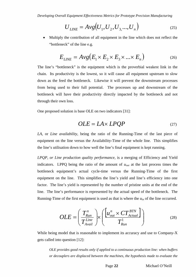
nLINE UUUUAvgU ...,,, ,321 (25)
Multiply the contribution of all equipment in the line which does not reflect the
“bottleneck” of the line e.g.
nLINE EEEEAvgE ...321 (26)
The line’s “bottleneck” is the equipment which is the proverbial weakest link in the
chain. Its productivity is the lowest, so it will cause all equipment upstream to slow
down as the feed the bottleneck. Likewise it will prevent the downstream processes
from being used to their full potential. The processes up and downstream of the
bottleneck will have their productivity directly impacted by the bottleneck and not
through their own loss.
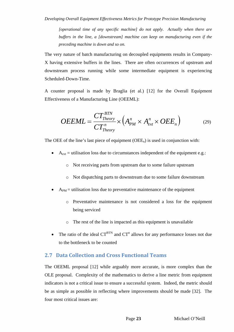
One proposed solution is base OLE on two indicators [31]:
LPQPLAOLE (27)
LA, or Line availability, being the ratio of the Running-Time of the last piece of
equipment on the line versus the Availability-Time of the whole line. This simplifies
the line’s utilisation down to how well the line’s final equipment is kept running.
LPQP, or Line production quality performance, is a merging of Efficiency and Yield
indicators. LPPQ being the ratio of the amount of uout at the last process times the
bottleneck equipment’s actual cycle-time versus the Running-Time of the first
equipment on the line. This simplifies the line’s yield and line’s efficiency into one
factor. The line’s yield is represented by the number of pristine units at the end of the
line. The line’s performance is represented by the actual speed of the bottleneck. The
Running-Time of the first equipment is used as that is where the uin of the line occurred.
1
Run
BTNActual
nout
LineAvail
nRun
T
CTu
T
TOLE
(28)
While being model that is reasonable to implement its accuracy and use to Company-X
gets called into question [12]:
OLE provides good results only if applied to a continuous production line: when buffers
or decouplers are displaced between the machines, the hypothesis made to evaluate the
Developing Overall Equipment Effectiveness Metrics for Prototype Precision Manufacturing
Page 23 Michael O’Neill
[operational time of any specific machine] do not apply. Actually when there are
buffers in the line, a [downstream] machine can keep on manufacturing even if the
preceding machine is down and so on.
The very nature of batch manufacturing on decoupled equipments results in Company-
X having extensive buffers in the lines. There are often occurrences of upstream and
downstream process running while some intermediate equipment is experiencing
Scheduled-Down-Time.
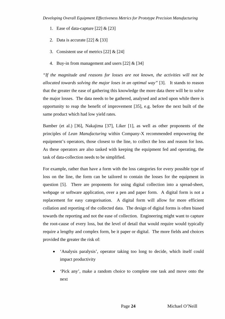
A counter proposal is made by Braglia (et al.) [12] for the Overall Equipment
Effectiveness of a Manufacturing Line (OEEML):
nnext
nPMn
Theory
BTNTheory OEEAA
CT
CTOEEML
(29)
The OEE of the line’s last piece of equipment (OEEn) is used in conjunction with:
Aext = utilisation loss due to circumstances independent of the equipment e.g.:
o Not receiving parts from upstream due to some failure upstream
o Not dispatching parts to downstream due to some failure downstream
APM = utilisation loss due to preventative maintenance of the equipment
o Preventative maintenance is not considered a loss for the equipment
being serviced
o The rest of the line is impacted as this equipment is unavailable
The ratio of the ideal CTBTN and CTn allows for any performance losses not due
to the bottleneck to be counted
2.7 DataCollectionandCrossFunctionalTeams
The OEEML proposal [12] while arguably more accurate, is more complex than the
OLE proposal. Complexity of the mathematics to derive a line metric from equipment
indicators is not a critical issue to ensure a successful system. Indeed, the metric should
be as simple as possible in reflecting where improvements should be made [32]. The
four most critical issues are:
Developing Overall Equipment Effectiveness Metrics for Prototype Precision Manufacturing
Page 24 Michael O’Neill
1. Ease of data-capture [22] & [23]
2. Data is accurate [22] & [33]
3. Consistent use of metrics [22] & [24]
4. Buy-in from management and users [22] & [34]
“If the magnitude and reasons for losses are not known, the activities will not be
allocated towards solving the major loses in an optimal way” [3]. It stands to reason
that the greater the ease of gathering this knowledge the more data there will be to solve
the major losses. The data needs to be gathered, analysed and acted upon while there is
opportunity to reap the benefit of improvement [35], e.g. before the next built of the
same product which had low yield rates.
Bamber (et al.) [36], Nakajima [37], Liker [1], as well as other proponents of the
principles of Lean Manufacturing within Company-X recommended empowering the
equipment’s operators, those closest to the line, to collect the loss and reason for loss.
As these operators are also tasked with keeping the equipment fed and operating, the
task of data-collection needs to be simplified.
For example, rather than have a form with the loss categories for every possible type of
loss on the line, the form can be tailored to contain the losses for the equipment in
question [5]. There are proponents for using digital collection into a spread-sheet,
webpage or software application, over a pen and paper form. A digital form is not a
replacement for easy categorisation. A digital form will allow for more efficient
collation and reporting of the collected data. The design of digital forms is often biased
towards the reporting and not the ease of collection. Engineering might want to capture
the root-cause of every loss, but the level of detail that would require would typically
require a lengthy and complex form, be it paper or digital. The more fields and choices
provided the greater the risk of:
‘Analysis paralysis’, operator taking too long to decide, which itself could
impact productivity
‘Pick any’, make a random choice to complete one task and move onto the
next
Developing Overall Equipment Effectiveness Metrics for Prototype Precision Manufacturing
Page 25 Michael O’Neill
With fewer choices, it is easier for multiple users to be consistent in their categorisation.
The challenge becomes how (or who) to decide on the categories. While many papers
cite Nakajima’s six major categories of loss [37], some individually recommend
specific interpretations. In comparing the whole they demonstrate difference in
interpretations. Bamber (et al.) [36] shows the importance of using cross-functional
teams (CFT) within a company to develop its “own classification framework for
losses”. Such a CFT could well be the same group tasked with improving productivity
based on the data gathered [20], and will be best positioned to perform the necessary
root-cause analysis [38].
This self-classification tends to relate to what the company’s personnel already
understand and is most likely to be maintained. This maintenance in turn will allow for
metrics, indicators and cause-data to be consistent. Consistency in turn will allow for
successful improvements to show up in the data. To this end, automation of the capture
and classification will ensure consistency [9] while eliminating tedious, manual tasks
[25]. Loughlin [39] recommends “Generation 3 OEE” system which integrates with the
equipments controller (PC and/or PLC) to capture indicators and potentially categorise
loss.
Even the OEE metric can be customised and tailored [34]. There are proponents of
different flavours of OEE for different applications [40]:
Simple OEE – Ratio of actual output versus theoretical output (same as
discussed in previous section)
Production OEE – OEE exclusive to production time, i.e. effectiveness of the
equipment when processing units
Demand OEE – OEE relative to the production schedule i.e. how effective the
equipment is used during scheduled activities
All these different applications underscore the idea that a company needs to choose the
classification and calculations that will allow them to learn and approve their
productivity. This in turn will lead to acceptance of the system by users, with is critical
for a system’s continued success.
Developing Overall Equipment Effectiveness Metrics for Prototype Precision Manufacturing
Page 26 Michael O’Neill
3 DevelopmentofLeanDataCollection
There is a paradox when it comes to data collection for equipment/process improvement
within a manufacturing facility either attempting to or practicing Lean Manufacturing
[1]. This will hereafter be referred to as the Information Paradox:
Actions based on good information are VALUE ADDED.
Actions to get good information are NON-VALUE ADDED.
While it is often acknowledged that there is waste inherent to any process that may
never be feasible to eliminate, the bigger issue is that data collection is often an after-
thought. The solution to break the Information Paradox is simple in concept: the
process must provide good information with no extra work. The act of physically
performing value-added tasks (work-flow) should result in the relevant data being
generated and collected (data-flow).
Company-X’s practices provide good illustration of how a process’s data-flow that is
disconnected from or done in addition to the process’s work-flow causes data-integrity
issues. Conversely, through leaning the process the data-flow can be integrated into the
work-flow.
3.1 InitialData‐collectionpractices
Company-X’s data-collection practice with respect to OEE is to capture and
characterize all incidents of yield loss and utilisation loss that occur on any given line.
A worst-case example best illustrates the waste present in their initial practice. The full
process in this example may not be used on every instance of loss but there is the
potential for it to occur.
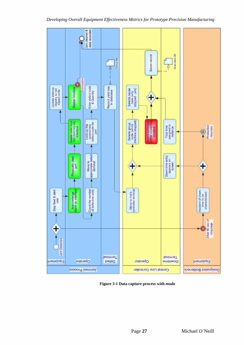
The business process model shown in Figure 3-1 represents the initial process with the
green squares showing the physical work the operator needs perform to get the
equipment operational.
Developing Overall Equipment Effectiveness Metrics for Prototype Precision Manufacturing
Page 27 Michael O’Neill
Figure 3-1 Data capture process with muda
Developing Overall Equipment Effectiveness Metrics for Prototype Precision Manufacturing
Page 28 Michael O’Neill
These practices have some key flaws that warrant address:
1. It was possible to detect a defect incident and not record it (red shape and
arrow in Figure 3-1’s Jammed Process / Operator region)
A. The operator was predisposed to remain monitoring the equipment where
the incident just occurred
B. The operator had to remember to move to the defect terminal and enter
the relevant information
C. If the distraction was due to another defect incident occurring, the initial
incident might never be recorded
2. It was possible to detect a downtime incident and inaccurately categorise it:
A. Operator had to travel from the equipment to a centralised computer
system to determine if the system detected a downtime incident greater
than ninety seconds
B. The operator tended to check a couple of time per shift, by which time
their memory of what caused each captured incident was poor.
C. Additionally, users had to type comments (red shape in Figure 3-1’s
Central Line Controller / Operator region) to provide enough detail to
categorise downtime incidents. This made the data highly inconsistent.
3. Only down-time incidents greater than ninety seconds were captured and
recorded (red shape in Figure 3-1’s Designated Bottleneck / Equipment
region)
A. This was an existing business rule at Company-X
B. On HVM lines any downtime lower than that was considered ‘minor’
loss and resulted in productivity losses that were not reflected in any
metric
4. The designed system had to be able to conclude that the need for all
downtime incidents to be captured did not result in over tasking operators
with data-collection activities.
Developing Overall Equipment Effectiveness Metrics for Prototype Precision Manufacturing
Page 29 Michael O’Neill
3.2 Leaningthedata‐collectionprocess
A cross-functional team was brought together to review the Initial Data-collection
practices in Figure 3-1 as a Kaizen event [1]. The first suggestion was to remove the
motion to other terminals to enter data by moving these terminals closer to the
equipment. These “extra” terminals were originally created when the equipment was
not networked and had no means to directly transmit data. Much of the equipment had
since been updated to utilise local and wide area networks. That allows recording to
and querying from databases. It was decided that rather than move a terminal with a
single tracking application, the application itself could be placed on the equipment’s
graphical user interface.
The next suggestion was to have the equipments’ software to record down-time
incidents automatically as well as defect incidents. As will be shown later, Company’s
X’s equipment has this capability, albeit in an inconsistent fashion. Additional
programming and sensors would add this capability to all equipment.
The only critical issue with this suggestion is that the equipment may not automatically
know the reason for which it is stopped. It will know that it is stopped and that units
have been removed from it. The operator will need to provide the reason. Rather than
type in the reason, the interface by which the operator provides this information can be
setup to provide only the relevant categorization for that equipment. The value of typed
comments was also demonstrated to be minimal and often used as a substitute for better
categorization.
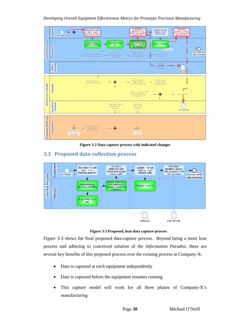
Figure 3-2 shows Company-X’s current processes with proposed changes that reflect
these ideas.
Developing Overall Equipment Effectiveness Metrics for Prototype Precision Manufacturing
Page 30 Michael O’Neill
Jam
med
Pro
cess
De
sig
nate
d B
ottle
ne
ck
Eq
uipm
en
t
Ce
ntr
al L
ine
Co
ntr
olle
r
Op
era
tor
De
fect
T
erm
ina
lD
own
time
Te
rmin
al
Op
era
tor
Jam Detected
Stop feed & alert user – start
tracking duration
Acknowledge alarm on interface
Physically clear jam
Delete units from m/c memory & choose reason
via interface
Update internal registry to not expect units
Restart Machine
Incident of down-time to be
characterizedProduction resumes
Count the number of defective units
Move to appropriate defect
terminal
Look-up the appropriate
defect-code for ‘jam’
Enter defect code & Quantity
Record yield loss in database
Move to line’s controller terminal
Down-time entry appears on
screen
Total time assigned to
instance
Selects group code (which
machine stopped)
Selects cause code (why
stopped - jam)
Enters comment further explaining
incidentSaves record
Jam cleared &data recorded
After 90 sec of stoppage
Eq
uip
men
t
Defect DB
Down-time DB
Distraction
Calculate defective unit
count and assign cause-code
Calculate duration, assign
m/c as group and jam as cause
Figure 3-2 Data capture process with indicated changes
3.3 Proposeddata‐collectionprocess
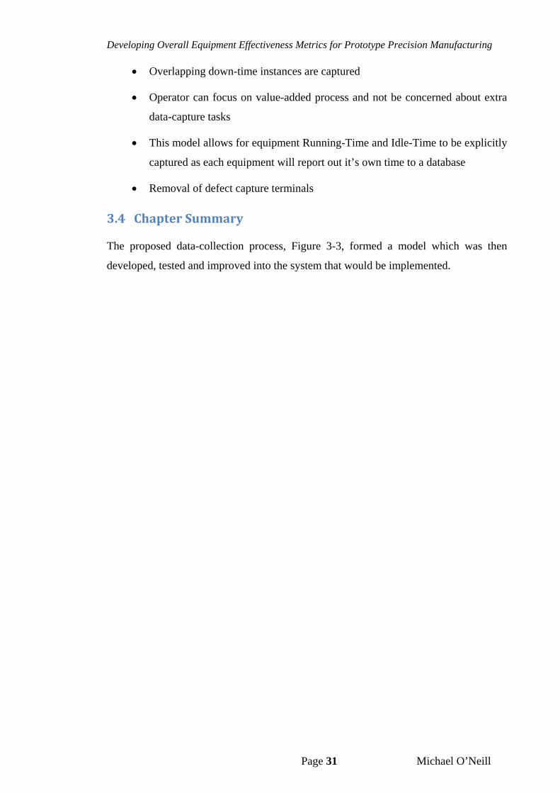
Figure 3-3 Proposed, lean data capture process
Figure 3-3 shows the final proposed data-capture process. Beyond being a more lean
process and adhering to conceived solution of the Information Paradox, there are
several key benefits of this proposed process over the existing process at Company-X:
Data is captured at each equipment independently
Data is captured before the equipment resumes running
This capture model will work for all three phases of Company-X’s
manufacturing
Developing Overall Equipment Effectiveness Metrics for Prototype Precision Manufacturing
Page 31 Michael O’Neill
Overlapping down-time instances are captured
Operator can focus on value-added process and not be concerned about extra
data-capture tasks
This model allows for equipment Running-Time and Idle-Time to be explicitly
captured as each equipment will report out it’s own time to a database
Removal of defect capture terminals
3.4 ChapterSummary
The proposed data-collection process, Figure 3-3, formed a model which was then
developed, tested and improved into the system that would be implemented.
Developing Overall Equipment Effectiveness Metrics for Prototype Precision Manufacturing
Page 32 Michael O’Neill
4 DevelopmentofUtilisationCapture
As the proposed Lean data-collection process, Figure 3-3, allowed for all time to be
captured and categorised, an indicator with explicit factors, Equations 7 & 9, were
chosen:
1. Time where the equipment is running i.e. processing units, TRun
2. Time where the equipment is idle, could have run but did not, TIdle e.g. lack
of units being feed into the equipment
3. Time where the equipment is unable to run due to some unscheduled event,
TUnschd
4. Time where the equipment is not run due to some scheduled event, TSchd
The issues affecting the accuracy of these factors will now be examined. Particular
emphasis will be placed on the issues which arose in developing the system for
Equipment-Z.
4.1 Timewheretheequipmentisrunning
Prior to this project, the only time captured within a Company-X line was the time a
designated piece of equipment in the line had stopped for a duration greater than ninety
seconds. Line Running-Time was inferred as calendar-time less all non-Running-Time.
Equipment Running-Time could similarly be inferred as the calendar-time less the all
non-Running-Time assigned to that particular equipment per Equation 6. This inference
would ignore any incidents were multiple pieces of equipment experience overlapping
or simultaneous downtime.
To address this inaccuracy, the Running-Time of each piece of equipment would have
to be explicitly captured. Equipment-Z was pre-programmed to understand when it was
running. The internal software sensed if:
There was a unit ready to be processed
There was an available space to unload the processed unit
All internal stations were ready to process
All the safety interlocks were closed
Developing Overall Equipment Effectiveness Metrics for Prototype Precision Manufacturing
Page 33 Michael O’Neill
The operator had pressed that start button
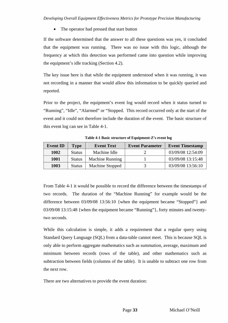
If the software determined that the answer to all these questions was yes, it concluded
that the equipment was running. There was no issue with this logic, although the
frequency at which this detection was performed came into question while improving
the equipment’s idle tracking (Section 4.2).
The key issue here is that while the equipment understood when it was running, it was
not recording in a manner that would allow this information to be quickly queried and
reported.
Prior to the project, the equipment’s event log would record when it status turned to
“Running”, “Idle”, “Alarmed” or “Stopped. This record occurred only at the start of the
event and it could not therefore include the duration of the event. The basic structure of
this event log can see in Table 4-1.
Table 4-1 Basic structure of Equipment-Z’s event log
Event ID Type Event Text Event Parameter Event Timestamp
1002 Status Machine Idle 2 03/09/08 12:54:09
1001 Status Machine Running 1 03/09/08 13:15:48
1003 Status Machine Stopped 3 03/09/08 13:56:10
From Table 4-1 it would be possible to record the difference between the timestamps of
two records. The duration of the “Machine Running” for example would be the
difference between 03/09/08 13:56:10 {when the equipment became “Stopped”} and
03/09/08 13:15:48 {when the equipment became “Running”}, forty minutes and twenty-
two seconds.
While this calculation is simple, it adds a requirement that a regular query using
Standard Query Language (SQL) from a data-table cannot meet. This is because SQL is
only able to perform aggregate mathematics such as summation, average, maximum and
minimum between records (rows of the table), and other mathematics such as
subtraction between fields (columns of the table). It is unable to subtract one row from
the next row.
There are two alternatives to provide the event duration:
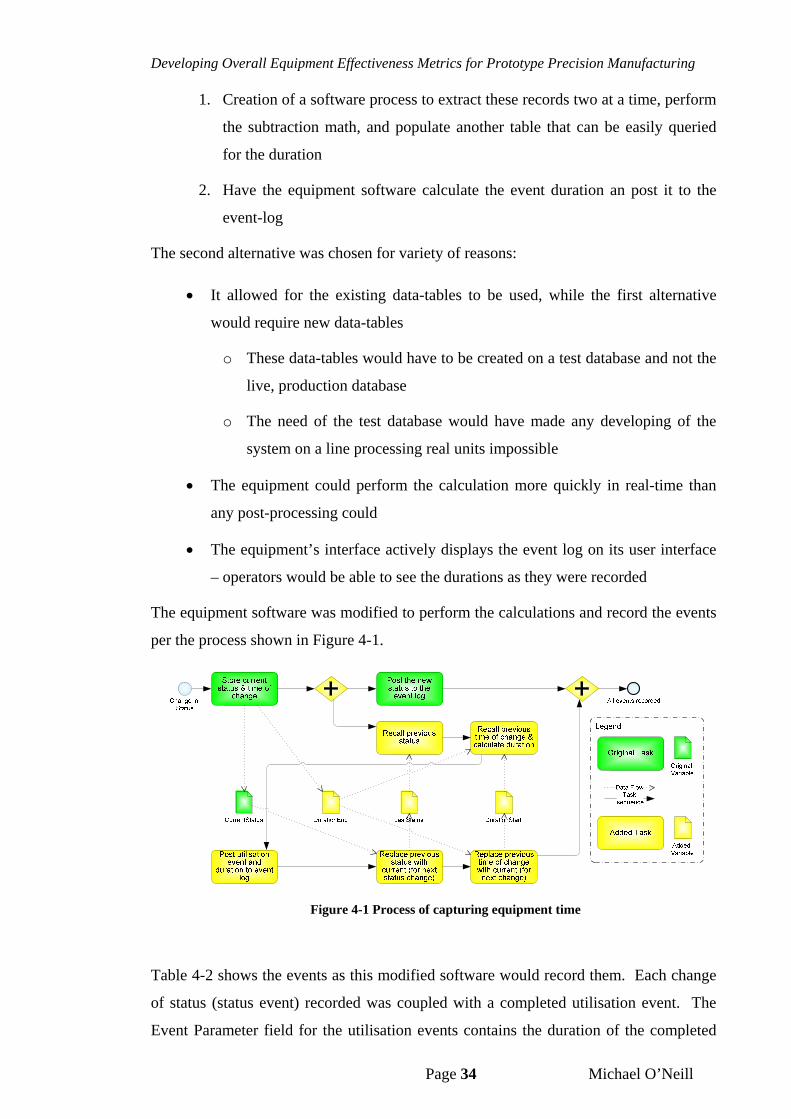
Developing Overall Equipment Effectiveness Metrics for Prototype Precision Manufacturing
Page 34 Michael O’Neill
1. Creation of a software process to extract these records two at a time, perform
the subtraction math, and populate another table that can be easily queried
for the duration
2. Have the equipment software calculate the event duration an post it to the
event-log
The second alternative was chosen for variety of reasons:
It allowed for the existing data-tables to be used, while the first alternative
would require new data-tables
o These data-tables would have to be created on a test database and not the
live, production database
o The need of the test database would have made any developing of the
system on a line processing real units impossible
The equipment could perform the calculation more quickly in real-time than
any post-processing could
The equipment’s interface actively displays the event log on its user interface
– operators would be able to see the durations as they were recorded
The equipment software was modified to perform the calculations and record the events
per the process shown in Figure 4-1.
Figure 4-1 Process of capturing equipment time
Table 4-2 shows the events as this modified software would record them. Each change
of status (status event) recorded was coupled with a completed utilisation event. The
Event Parameter field for the utilisation events contains the duration of the completed
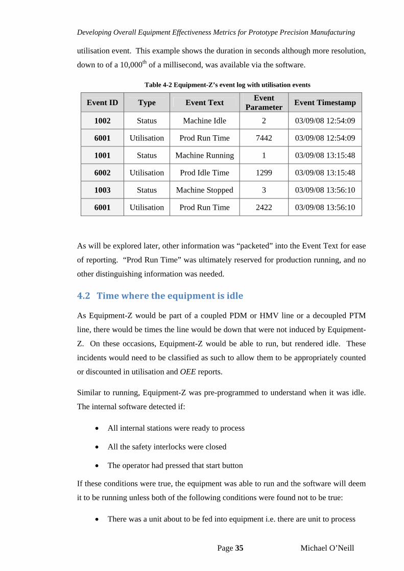
Developing Overall Equipment Effectiveness Metrics for Prototype Precision Manufacturing
Page 35 Michael O’Neill
utilisation event. This example shows the duration in seconds although more resolution,
down to of a 10,000th of a millisecond, was available via the software.
Table 4-2 Equipment-Z’s event log with utilisation events
Event ID Type Event Text Event
Parameter Event Timestamp
1002 Status Machine Idle 2 03/09/08 12:54:09
6001 Utilisation Prod Run Time 7442 03/09/08 12:54:09
1001 Status Machine Running 1 03/09/08 13:15:48
6002 Utilisation Prod Idle Time 1299 03/09/08 13:15:48
1003 Status Machine Stopped 3 03/09/08 13:56:10
6001 Utilisation Prod Run Time 2422 03/09/08 13:56:10
As will be explored later, other information was “packeted” into the Event Text for ease
of reporting. “Prod Run Time” was ultimately reserved for production running, and no
other distinguishing information was needed.
4.2 Timewheretheequipmentisidle
As Equipment-Z would be part of a coupled PDM or HMV line or a decoupled PTM
line, there would be times the line would be down that were not induced by Equipment-
Z. On these occasions, Equipment-Z would be able to run, but rendered idle. These
incidents would need to be classified as such to allow them to be appropriately counted
or discounted in utilisation and OEE reports.
Similar to running, Equipment-Z was pre-programmed to understand when it was idle.
The internal software detected if:
All internal stations were ready to process
All the safety interlocks were closed
The operator had pressed that start button
If these conditions were true, the equipment was able to run and the software will deem
it to be running unless both of the following conditions were found not to be true:
There was a unit about to be fed into equipment i.e. there are unit to process
Developing Overall Equipment Effectiveness Metrics for Prototype Precision Manufacturing
Page 36 Michael O’Neill
Completed units could be unloaded from the equipment i.e. the equipment
could feed units to each internal operation
If both were not true, the software concluded the equipment was idle.
It was determined that this idle condition was only relevant during scheduled production
runs as it would point to incidents when either units were not being fed or input to the
equipment, or incidents were the equipment was unable to feed or output units. The
former would point the cause to some ‘upstream’ cause, i.e. some issue had occurred to
an equipment or process that precedes this equipment. The latter would point the cause
to some ‘downstream’ cause, i.e. some issue had occurred to a piece of equipment or
process that proceeds this equipment. Another potential source of the idle condition
would be that operator has instructed the equipment to ‘run out’ or ‘clean-out’, which
would instruct it not to take in new units and continue to process existing units.
This classification of ‘idle due to upstream or downstream failure’ or ‘operator directed’
needed to be included into Event Text. Equipment-Z’s software utilized many input-
output signals (I/O) to make decisions. These same I/O were also used to determine the
source of the idle condition and in certain circumstances provide the reason for the idle
incident.
This programmed logic was used to create three elements comprising the Event Text
output to the database:
Utilisation event category
Utilisation event reason
Utilisation event sub-reason
The Event Text string delimited these elements by separating them with a vertical bar
character “|” (ASCII code 124) as this character was not used in any other entries posted
to the event log and could therefore be reliably used to separate out the elements in
reporting. The format of the Event Text string would be “Category | Reason | Sub-
reason”. Table 4-3 shows the categorisation used for the category of ‘Prod Idle Time’.

Developing Overall Equipment Effectiveness Metrics for Prototype Precision Manufacturing
Page 37 Michael O’Neill
Table 4-3 Example of reasons (cause) of idle events
Event Reason Event Sub-Reason
Auto Idle as there is no Product to Process
No units from upstream
Upstream (master feed) process is idle or stopped
Upstream (master feed) process is stopped
User selected cleanout
Auto Idle as unable to Process Product
Downstream (slave feed) process is idle or stopped
Downstream (slave feed) process is stopped
Unable to unload units downstream
Upstream (master feed) process is idle or stopped
Upstream (master feed) process is stopped
Auto Idle due to Downstream Process
Unable to unload units downstream
Auto Idle due to unknown Cause of idle condition is unknown
Auto Idle due to Upstream Process
No units from upstream
User selected to Clean Out Module
Reason for Clean Out is unknown
Equipment-Z‘s pre-existing code was the key source of inaccuracy in determining idle-
time.
An independent software timer was used as such that every sixty seconds the software
would determine if the equipment was processing units. It did this by looking at the I/O
that signalled if all stations within the equipment were ready to process a unit. If all
were, the I/O would be set to TRUE and the logic would determine the equipment to be
idle. If any were not, the I/O would be set to FALSE and the logic would determine the
equipment to be running.
The sixty second interval of this timer resulted in an up to sixty seconds delay from
when the equipment truly became idle (or running) to when the software logic
determined this occurrence. In addition to the delay, the I/O would cycle from FALSE
to TRUE to FALSE and so on, on every cycle of the equipment’s feed-line. As this
Developing Overall Equipment Effectiveness Metrics for Prototype Precision Manufacturing
Page 38 Michael O’Neill
cycling was independent of the sensing timer, the detection of an idle condition was
matter of coincidence rather than discerning logic.
Two changes were needed to address this circumstance:
1. Decrease the sensing timer to a shorter interval
2. Develop discriminating logic to determine when the process is idle
The timed-interval was dropped to one second as that was deemed to provide enough
resolution for time tracking without impacting the cycle-time of the equipment.
Testing revealed that this rendered the code overly sensitive with the effect of every
second or so, the utilisation-tracking software would cycle between running events and
idle events. With the logic used, the equipment became idle for a portion of every
machine-cycle just before it indexed a new unit into the equipment. Detection of this
temporary idle-state was not valuable to characterising utilisation as Equipment-Z never
actually stopped processing. As this pause was an inherent part of the machine-cycle it
represented an efficiency loss rather than an utilisation loss.
To desensitise the utilisation logic to this pause, an additional input was added whereby
the duration of this pause was analysed. If the duration exceeded a specified limit
chosen to reflect the inherent efficiency loss, the equipment would be determined as
idle. The question became what should be used as the value of this limit?
Under normal running, this pause would not last more than a few tenths of second.
However, the duration of the pause was variable depending on what upstream
equipment Equipment-Z was coupled to. As the software was written such that it could
be ported to equipment other than Equipment-Z, it was simpler to set the allowable
duration to a fixed number. This simplification also allowed for a more efficient
processing time of the software. Short processing time is important as to ensure
negligible impact to equipment cycle-time.
4.3 Time where the equipment is unable to run due to some
unscheduledevent
The system had to handle two key types of stoppages during production running:
1. Those triggered by Equipment-Z’s internal controls
2. Those triggered by the operator
Developing Overall Equipment Effectiveness Metrics for Prototype Precision Manufacturing
Page 39 Michael O’Neill
4.3.1 Equipmenttriggeredunscheduledevent
With its internal sensors and in-line process control mechanisms, Equipment-Z was able
to alarm and stop itself whenever its software detected an inappropriate condition. This
automatic stopping (or auto stop) provided the opportunity for the software to
immediately detect and categorise the reason for the Unscheduled Down-Time event.
Upon occurrence of these alarms, the utilisation-tracking software would define the
Event Category as “Unscheduled Down Time”, the Event Reason as “Auto stop due to
alarm from [appropriate station within Equipment-Z]”, and the Event Sub-reason would
use the same verbiage used in the alarm’s pop-up displayed on the equipment’s
interface to the operator.
While being a simple requirement to program into the utilisation-tracking software, it
immediately proved to be a powerful tool. In the past, Company-X’s maintenance
department reported on the number of occurrences of alarms to prioritise improvement
opportunities. For the first time, the utilisation software provided the opportunity to
quantify the impact of each alarm.
The pre-existing utilisation-tracking system only identified down-time events greater
than ninety seconds. In the PTM and PDM lines, it would be common occurrence
where the in-line control limits used in Equipment-Z for a given product were based on
limits used on a product that had matured to HVM. These limits would not reflect the
capability of the program in PTM and PDM and would effectively alarm and stop the
equipment in circumstances were no action should be undertaken.
These “false calls”, or Type II errors, were a source of contention between
manufacturing, manufacturing support and process engineering. It is the remit of
process engineers to set the limits of the in-line process controls. Not understanding the
impact of these false calls to manufacturing, the engineers would procrastinate on
updating the equipment’s settings and merely instruct manufacturing to ignore the
alarms. However, an ignored alarm would still have to be cleared by an operator and
then the equipment restarted. As this acknowledging and clearing of the alarm and
resuming of equipment typically took far less than ninety seconds, scores of these
alarms could occur on a given crew and never be reflected in the existing performance
metrics.
Developing Overall Equipment Effectiveness Metrics for Prototype Precision Manufacturing
Page 40 Michael O’Neill
While not within the subject matter of this project, it is worth pointing out these “clear
and go” practices also lead to valid alarms being accidentally cleared without proper
response and various internal and external quality incidents.
4.3.2 Operatortriggeredunscheduledevent
Within normal process running there will be incidents that require the operator to
manually stop the equipment:
Performing a process control check
Removing units (jam, sampling, etc)
Changing a manufacturing order
Responding to off-line process control trend or failure
Start of a non-production event (Scheduled-Down-Time)
To ensure that the appropriate cause information is captured, and that the capture
method is compliant with the proposed process model in Figure 2-1, a mechanism had
to be developed to ensure that the cause information was captured before running of the
equipment could be resumed.
With Equipment-Z’s current interface, the operator would need to press specific buttons
to remove units, perform a process control check or change a manufacturing order.
With this known, the utilisation-tracking software was able to detect these button
presses and use these occurrences to categorise the reason (and sub-reason) for the
stoppage triggered by the operator (or any user). Each occurrence of a button press
resulted in the software tracking a new utilisation event.
No specific pre-existing interface buttons were required to be pressed to respond to
process control trend or failure, or the start of a non-production event. For that reason it
became necessary for the utilisation-tracking software to prompt the user to select the
appropriate reason for the stoppage. As the user could select the wrong option, this lack
of automation posed a compromise to the integrity of captured data.
A cross-functional team (CFT) of manufacturing, training and engineering personnel
was created with representatives from each of the Company-X’s PTM, PDM and HVM-
focused plants. The developing system was installed in Equipment-Z on selected lines
to allow the team to interact with the system. Daily reviews were undertaken to
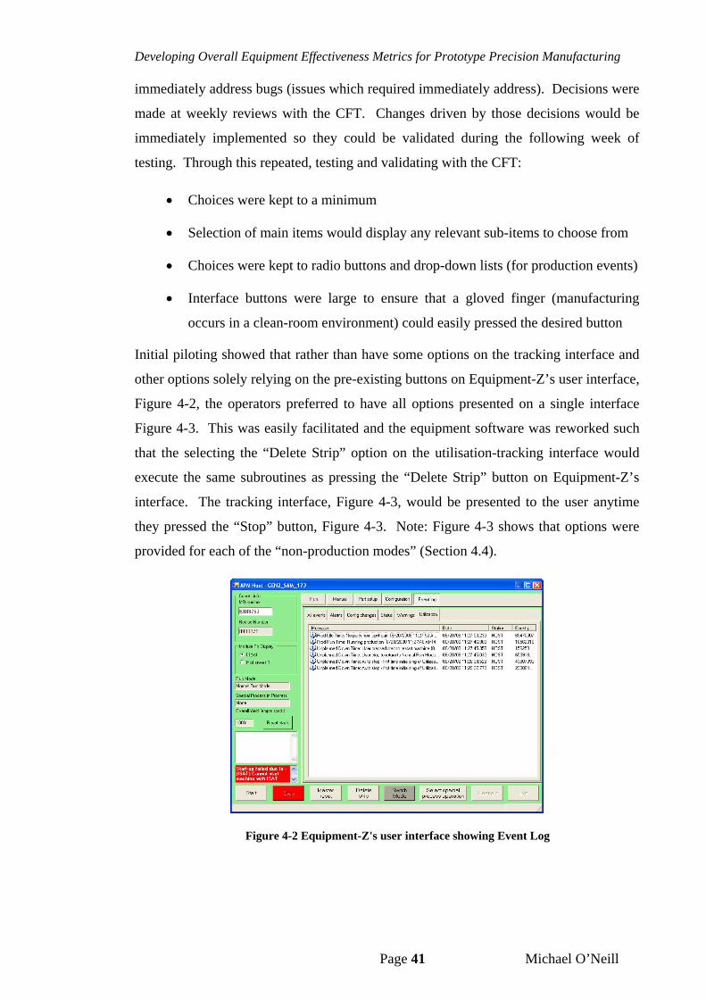
Developing Overall Equipment Effectiveness Metrics for Prototype Precision Manufacturing
Page 41 Michael O’Neill
immediately address bugs (issues which required immediately address). Decisions were
made at weekly reviews with the CFT. Changes driven by those decisions would be
immediately implemented so they could be validated during the following week of
testing. Through this repeated, testing and validating with the CFT:
Choices were kept to a minimum
Selection of main items would display any relevant sub-items to choose from
Choices were kept to radio buttons and drop-down lists (for production events)
Interface buttons were large to ensure that a gloved finger (manufacturing
occurs in a clean-room environment) could easily pressed the desired button
Initial piloting showed that rather than have some options on the tracking interface and
other options solely relying on the pre-existing buttons on Equipment-Z’s user interface,
Figure 4-2, the operators preferred to have all options presented on a single interface
Figure 4-3. This was easily facilitated and the equipment software was reworked such
that the selecting the “Delete Strip” option on the utilisation-tracking interface would
execute the same subroutines as pressing the “Delete Strip” button on Equipment-Z’s
interface. The tracking interface, Figure 4-3, would be presented to the user anytime
they pressed the “Stop” button, Figure 4-3. Note: Figure 4-3 shows that options were
provided for each of the “non-production modes” (Section 4.4).
Figure 4-2 Equipment-Z's user interface showing Event Log
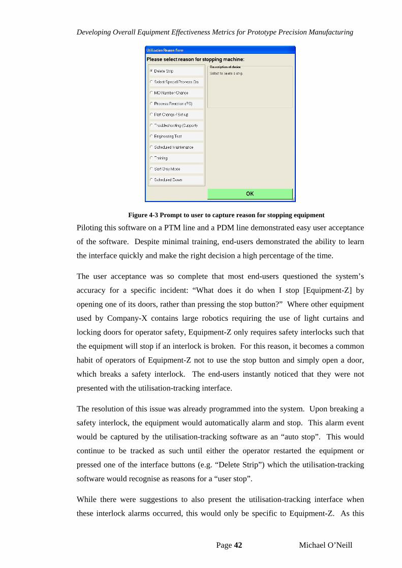
Developing Overall Equipment Effectiveness Metrics for Prototype Precision Manufacturing
Page 42 Michael O’Neill
Figure 4-3 Prompt to user to capture reason for stopping equipment
Piloting this software on a PTM line and a PDM line demonstrated easy user acceptance
of the software. Despite minimal training, end-users demonstrated the ability to learn
the interface quickly and make the right decision a high percentage of the time.
The user acceptance was so complete that most end-users questioned the system’s
accuracy for a specific incident: “What does it do when I stop [Equipment-Z] by
opening one of its doors, rather than pressing the stop button?” Where other equipment
used by Company-X contains large robotics requiring the use of light curtains and
locking doors for operator safety, Equipment-Z only requires safety interlocks such that
the equipment will stop if an interlock is broken. For this reason, it becomes a common
habit of operators of Equipment-Z not to use the stop button and simply open a door,
which breaks a safety interlock. The end-users instantly noticed that they were not
presented with the utilisation-tracking interface.
The resolution of this issue was already programmed into the system. Upon breaking a
safety interlock, the equipment would automatically alarm and stop. This alarm event
would be captured by the utilisation-tracking software as an “auto stop”. This would
continue to be tracked as such until either the operator restarted the equipment or
pressed one of the interface buttons (e.g. “Delete Strip”) which the utilisation-tracking
software would recognise as reasons for a “user stop”.
While there were suggestions to also present the utilisation-tracking interface when
these interlock alarms occurred, this would only be specific to Equipment-Z. As this
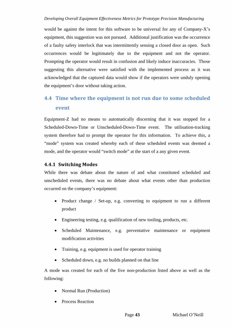
Developing Overall Equipment Effectiveness Metrics for Prototype Precision Manufacturing
Page 43 Michael O’Neill
would be against the intent for this software to be universal for any of Company-X’s
equipment, this suggestion was not pursued. Additional justification was the occurrence
of a faulty safety interlock that was intermittently sensing a closed door as open. Such
occurrences would be legitimately due to the equipment and not the operator.
Prompting the operator would result in confusion and likely induce inaccuracies. Those
suggesting this alternative were satisfied with the implemented process as it was
acknowledged that the captured data would show if the operators were unduly opening
the equipment’s door without taking action.
4.4 Timewheretheequipmentisnotrunduetosomescheduled
event
Equipment-Z had no means to automatically discerning that it was stopped for a
Scheduled-Down-Time or Unscheduled-Down-Time event. The utilisation-tracking
system therefore had to prompt the operator for this information. To achieve this, a
“mode” system was created whereby each of these scheduled events was deemed a
mode, and the operator would “switch mode” at the start of a any given event.
4.4.1 SwitchingModes
While there was debate about the nature of and what constituted scheduled and
unscheduled events, there was no debate about what events other than production
occurred on the company’s equipment:
Product change / Set-up, e.g. converting to equipment to run a different
product
Engineering testing, e.g. qualification of new tooling, products, etc.
Scheduled Maintenance, e.g. preventative maintenance or equipment
modification activities
Training, e.g. equipment is used for operator training
Scheduled down, e.g. no builds planned on that line
A mode was created for each of the five non-production listed above as well as the
following:
Normal Run (Production)
Process Reaction
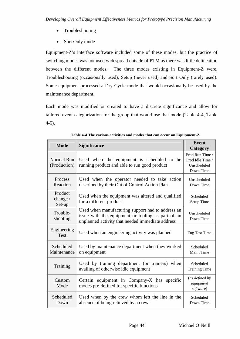
Developing Overall Equipment Effectiveness Metrics for Prototype Precision Manufacturing
Page 44 Michael O’Neill
Troubleshooting
Sort Only mode
Equipment-Z’s interface software included some of these modes, but the practice of
switching modes was not used widespread outside of PTM as there was little delineation
between the different modes. The three modes existing in Equipment-Z were,
Troubleshooting (occasionally used), Setup (never used) and Sort Only (rarely used).
Some equipment processed a Dry Cycle mode that would occasionally be used by the
maintenance department.
Each mode was modified or created to have a discrete significance and allow for
tailored event categorization for the group that would use that mode (Table 4-4, Table
4-5).
Table 4-4 The various activities and modes that can occur on Equipment-Z
Mode Significance Event
Category
Normal Run (Production)
Used when the equipment is scheduled to be running product and able to run good product
Prod Run Time /Prod Idle Time /
Unscheduled Down Time
Process Reaction
Used when the operator needed to take action described by their Out of Control Action Plan
Unscheduled Down Time
Product change / Set-up
Used when the equipment was altered and qualified for a different product
Scheduled Setup Time
Trouble-shooting
Used when manufacturing support had to address an issue with the equipment or tooling as part of an unplanned activity that needed immediate address
Unscheduled Down Time
Engineering Test
Used when an engineering activity was planned Eng Test Time
Scheduled Maintenance
Used by maintenance department when they worked on equipment
Scheduled Maint Time
Training Used by training department (or trainers) when availing of otherwise idle equipment
Scheduled Training Time
Custom Mode
Certain equipment in Company-X has specific modes pre-defined for specific functions
(as defined by equipment software)
Scheduled Down
Used when by the crew whom left the line in the absence of being relieved by a crew
Scheduled Down Time
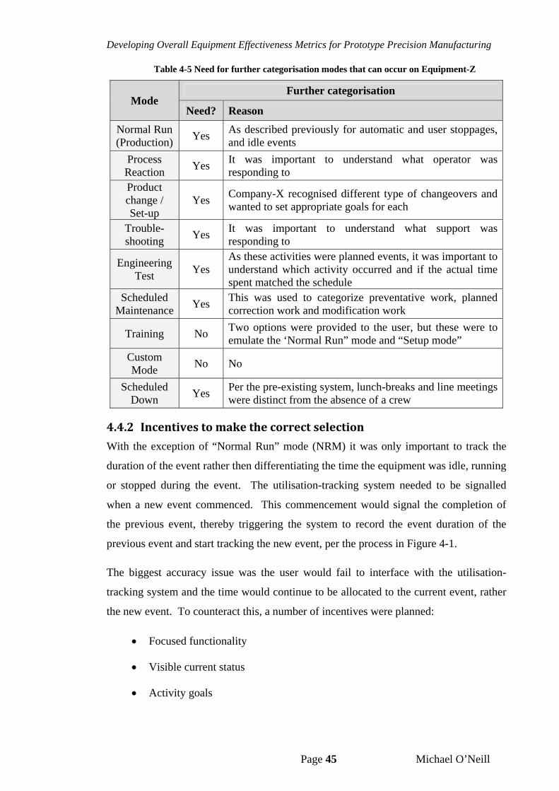
Developing Overall Equipment Effectiveness Metrics for Prototype Precision Manufacturing
Page 45 Michael O’Neill
Table 4-5 Need for further categorisation modes that can occur on Equipment-Z
Mode Further categorisation
Need? Reason
Normal Run (Production)
Yes As described previously for automatic and user stoppages, and idle events
Process Reaction
Yes It was important to understand what operator was responding to
Product change / Set-up
Yes Company-X recognised different type of changeovers and wanted to set appropriate goals for each
Trouble-shooting
Yes It was important to understand what support was responding to
Engineering Test
Yes As these activities were planned events, it was important to understand which activity occurred and if the actual time spent matched the schedule
Scheduled Maintenance
Yes This was used to categorize preventative work, planned correction work and modification work
Training No Two options were provided to the user, but these were to emulate the ‘Normal Run” mode and “Setup mode”
Custom Mode
No No
Scheduled Down
Yes Per the pre-existing system, lunch-breaks and line meetings were distinct from the absence of a crew
4.4.2 Incentivestomakethecorrectselection
With the exception of “Normal Run” mode (NRM) it was only important to track the
duration of the event rather then differentiating the time the equipment was idle, running
or stopped during the event. The utilisation-tracking system needed to be signalled
when a new event commenced. This commencement would signal the completion of
the previous event, thereby triggering the system to record the event duration of the
previous event and start tracking the new event, per the process in Figure 4-1.
The biggest accuracy issue was the user would fail to interface with the utilisation-
tracking system and the time would continue to be allocated to the current event, rather
the new event. To counteract this, a number of incentives were planned:
Focused functionality
Visible current status
Activity goals
Developing Overall Equipment Effectiveness Metrics for Prototype Precision Manufacturing
Page 46 Michael O’Neill
4.4.3 Focusedfunctionality
The interface of Equipment-Z provided a lot of functionality to the operator, as well as
any support personnel. As can been seen in Figure 4-4, all of the functions needed
during normal production running were immediately accessible. These are dubbed
“basic functions”. The various tabs and buttons on the upper portion of the interface
allowed for viewing of the equipments settings, manual control screen and in-line
control status. These screens provided functions where by the user could change a
setting or manually index the feed-line or change the position of a motor-controlled
stage. These functions are dubbed “additional functions” as they would not be typically
used during normal production.
Figure 4-4 Basic & Additional function of Equipment-Z's interface
Unlike other equipment in Company-X, Equipment-Z’s interface did not require a
password to access these additional functions. These were readily available at any time
except when the equipment was actively processing units. At such time, the interface
was disabled such that the user could view the screens, but not trigger any of the
functions.
As these additional functions were not pertinent to a production event, the equipment
interface software was altered to disable the additional functions while the equipment
was in Normal Run Mode. These additional functions would only be enabled when the
user switched the equipment’s mode to denote an activity whereby these functions were
required.
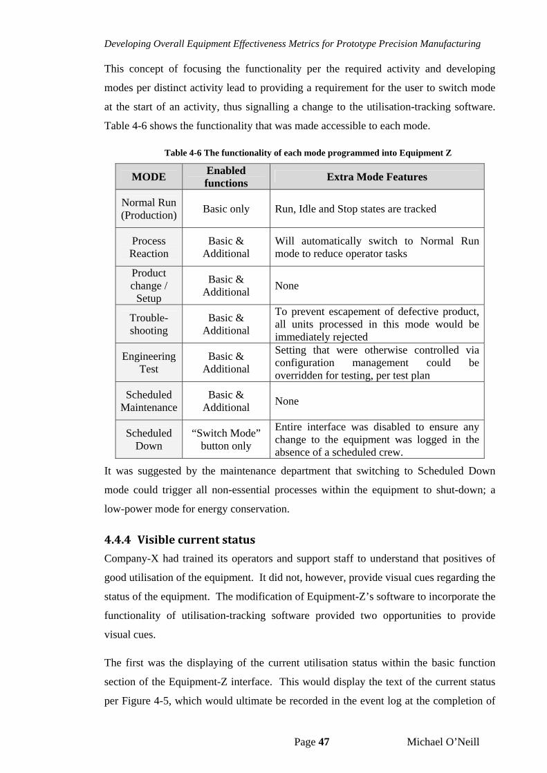
Developing Overall Equipment Effectiveness Metrics for Prototype Precision Manufacturing
Page 47 Michael O’Neill
This concept of focusing the functionality per the required activity and developing
modes per distinct activity lead to providing a requirement for the user to switch mode
at the start of an activity, thus signalling a change to the utilisation-tracking software.
Table 4-6 shows the functionality that was made accessible to each mode.
Table 4-6 The functionality of each mode programmed into Equipment Z
MODE Enabled functions
Extra Mode Features
Normal Run (Production)
Basic only Run, Idle and Stop states are tracked
Process Reaction
Basic & Additional
Will automatically switch to Normal Run mode to reduce operator tasks
Product change /
Setup
Basic & Additional
None
Trouble-shooting
Basic & Additional
To prevent escapement of defective product, all units processed in this mode would be immediately rejected
Engineering Test
Basic & Additional
Setting that were otherwise controlled via configuration management could be overridden for testing, per test plan
Scheduled Maintenance
Basic & Additional
None
Scheduled Down
“Switch Mode” button only
Entire interface was disabled to ensure any change to the equipment was logged in the absence of a scheduled crew.
It was suggested by the maintenance department that switching to Scheduled Down
mode could trigger all non-essential processes within the equipment to shut-down; a
low-power mode for energy conservation.
4.4.4 Visiblecurrentstatus
Company-X had trained its operators and support staff to understand that positives of
good utilisation of the equipment. It did not, however, provide visual cues regarding the
status of the equipment. The modification of Equipment-Z’s software to incorporate the
functionality of utilisation-tracking software provided two opportunities to provide
visual cues.
The first was the displaying of the current utilisation status within the basic function
section of the Equipment-Z interface. This would display the text of the current status
per Figure 4-5, which would ultimate be recorded in the event log at the completion of
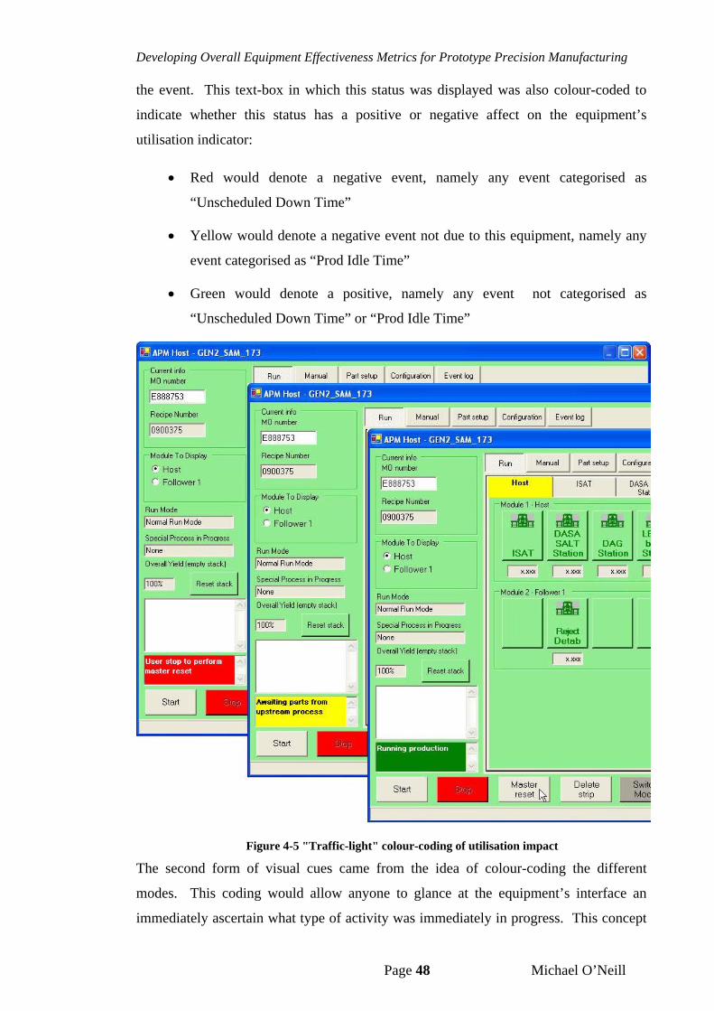
Developing Overall Equipment Effectiveness Metrics for Prototype Precision Manufacturing
Page 48 Michael O’Neill
the event. This text-box in which this status was displayed was also colour-coded to
indicate whether this status has a positive or negative affect on the equipment’s
utilisation indicator:
Red would denote a negative event, namely any event categorised as
“Unscheduled Down Time”
Yellow would denote a negative event not due to this equipment, namely any
event categorised as “Prod Idle Time”
Green would denote a positive, namely any event not categorised as
“Unscheduled Down Time” or “Prod Idle Time”
Figure 4-5 "Traffic-light" colour-coding of utilisation impact
The second form of visual cues came from the idea of colour-coding the different
modes. This coding would allow anyone to glance at the equipment’s interface an
immediately ascertain what type of activity was immediately in progress. This concept
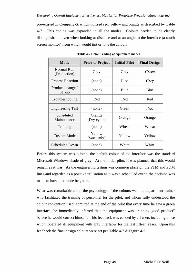
Developing Overall Equipment Effectiveness Metrics for Prototype Precision Manufacturing
Page 49 Michael O’Neill
pre-existed in Company-X which utilized red, yellow and orange as described by Table
4-7. This coding was expanded to all the modes. Colours needed to be clearly
distinguishable even when looking at distance and at an angle to the interface (a touch
screen monitor) from which would tint or tone the colour.
Table 4-7 Colour-coding of equipment modes
Mode Prior to Project Initial Pilot Final Design
Normal Run (Production)
Grey Grey Green
Process Reaction (none) Iliac Grey
Product change / Set-up
(none) Blue Blue
Troubleshooting Red Red Red
Engineering Test (none) Green Iliac
Scheduled Maintenance
Orange {Dry cycle}
Orange Orange
Training (none) Wheat Wheat
Custom Mode Yellow
{Sort Only} Yellow Yellow
Scheduled Down (none) White White
Before this system was piloted, the default colour of the interface was the standard
Microsoft Windows shade of grey. At the initial pilot, it was planned that this would
remain as it was. As the engineering testing was common place on the PTM and PDM
lines and regarded as a positive utilisation as it was a scheduled event, the decision was
made to have that mode be green.
What was remarkable about the psychology of the colours was the department trainer
who facilitated the training of personnel for the pilot, and whom fully understood the
colour convention used, admitted at the end of the pilot that every time he saw a green
interface, he immediately inferred that the equipment was “running good product”
before he would correct himself. This feedback was echoed by all users including those
whom operated all equipment with gray interfaces for the last fifteen years. Upon this
feedback the final design colours were set per Table 4-7 & Figure 4-6.
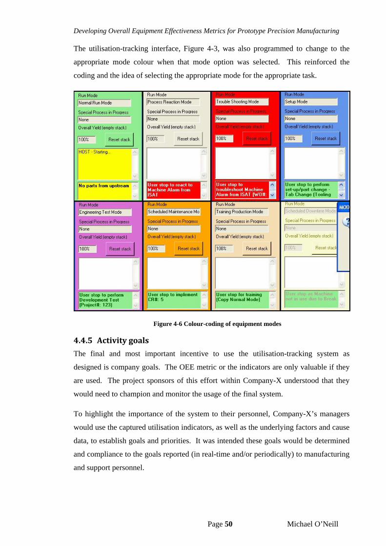
Developing Overall Equipment Effectiveness Metrics for Prototype Precision Manufacturing
Page 50 Michael O’Neill
The utilisation-tracking interface, Figure 4-3, was also programmed to change to the
appropriate mode colour when that mode option was selected. This reinforced the
coding and the idea of selecting the appropriate mode for the appropriate task.
Figure 4-6 Colour-coding of equipment modes
4.4.5 Activitygoals
The final and most important incentive to use the utilisation-tracking system as
designed is company goals. The OEE metric or the indicators are only valuable if they
are used. The project sponsors of this effort within Company-X understood that they
would need to champion and monitor the usage of the final system.
To highlight the importance of the system to their personnel, Company-X’s managers
would use the captured utilisation indicators, as well as the underlying factors and cause
data, to establish goals and priorities. It was intended these goals would be determined
and compliance to the goals reported (in real-time and/or periodically) to manufacturing
and support personnel.
Developing Overall Equipment Effectiveness Metrics for Prototype Precision Manufacturing
Page 51 Michael O’Neill
Some of examples of this reporting and prioritising were conceptualised during this
project by the targeted end-users. Numbers are provided below to highlight the
concept:
Manufacturing department:
o Utilisation per manufacturing order exceeding 90%
o Software changeover in under 1 hours
o Tab to tab changeover in under 2 hours
o Full tooling changeover in under 8 hours
Training department:
o 100% of scheduled activities completed as schedules per week
Maintenance department:
o 100% of scheduled activities completed as schedules per week
o 5% reduction in troubleshooting events on Equipment-Z by end of fiscal
year.
Engineering department:
o 100% of scheduled activities completed as schedules per week
o Improve Equipment-Z’s utilisation by 5% by end of fiscal year
4.5 Reliability
Beyond the accuracy issues relating to the capture of each of the factors, two issues of
reliable capture of the data arose. The first was that time would have to be tracked even
when the equipment was powered down. The equipment’s software and hardware
performed the tracking and powering down was a common requirement of maintenance
activities.
The second was that recording the data only when a new event commenced would be
not provide reliable real-time feedback. For example a twelve-hour event of Scheduled
Down-Time would only be recorded on the twelfth hour with no record of the current
event during the first to eleventh hour.
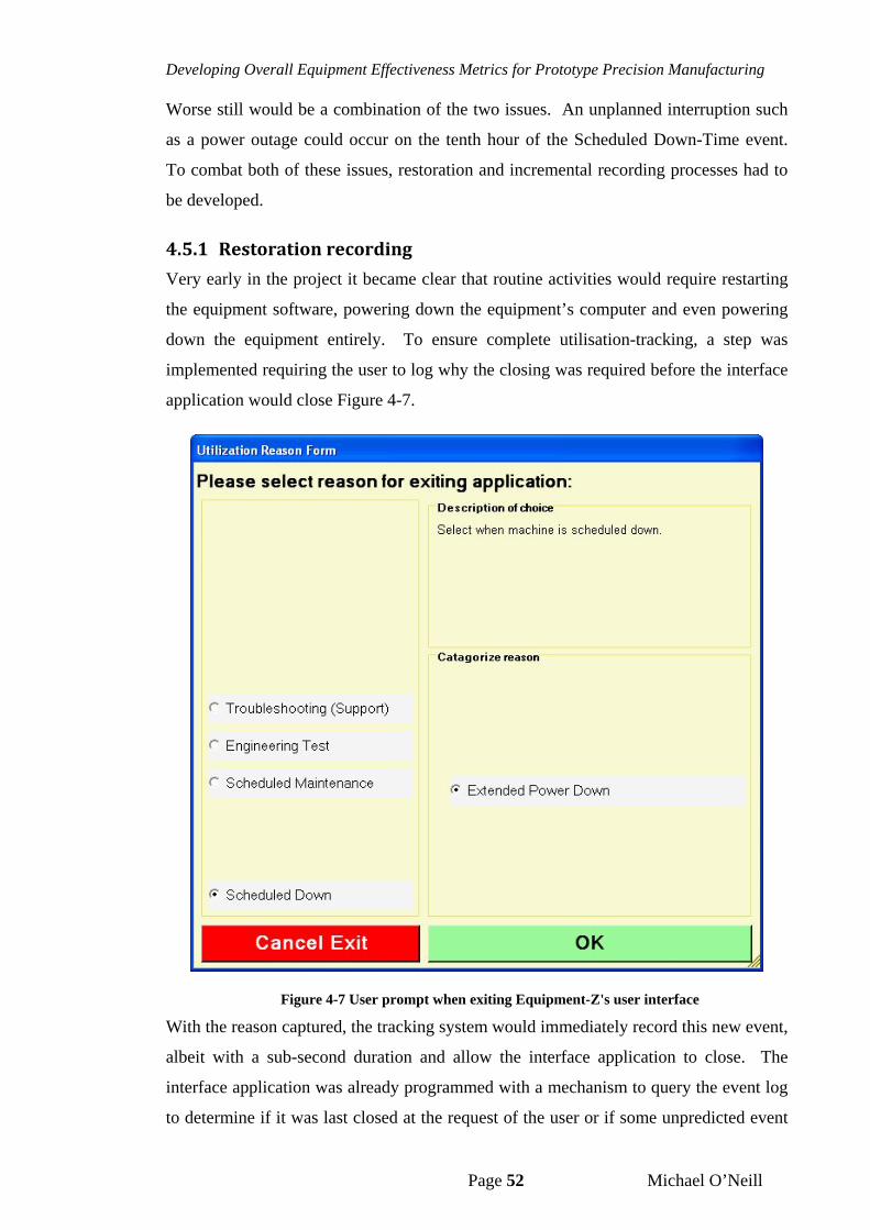
Developing Overall Equipment Effectiveness Metrics for Prototype Precision Manufacturing
Page 52 Michael O’Neill
Worse still would be a combination of the two issues. An unplanned interruption such
as a power outage could occur on the tenth hour of the Scheduled Down-Time event.
To combat both of these issues, restoration and incremental recording processes had to
be developed.
4.5.1 Restorationrecording
Very early in the project it became clear that routine activities would require restarting
the equipment software, powering down the equipment’s computer and even powering
down the equipment entirely. To ensure complete utilisation-tracking, a step was
implemented requiring the user to log why the closing was required before the interface
application would close Figure 4-7.
Figure 4-7 User prompt when exiting Equipment-Z's user interface
With the reason captured, the tracking system would immediately record this new event,
albeit with a sub-second duration and allow the interface application to close. The
interface application was already programmed with a mechanism to query the event log
to determine if it was last closed at the request of the user or if some unpredicted event
Developing Overall Equipment Effectiveness Metrics for Prototype Precision Manufacturing
Page 53 Michael O’Neill
occurred. This programming was expanded to query the last captured utilisation event.
If the application was properly closed, the last event would be that immediately
recorded prior to the application being terminated.
With this last utilisation event known, the same category, reason, sub-reason and event
timestamp could immediately be used by the utilisation-tracking software. The
software was able to calculate the duration the application was down via the current
time and the record’s timestamp. Upon making this calculation, the system would
immediately:
1. Record this “turned-off” event
2. Restore the application to the same mode it was in prior to requested close
out
3. Resume the tracking of the activity which prompted the termination
If upon restart of the application, the software determined that the application was not
properly terminated i.e. it was not requested by the user, the utilisation-tracking
software would prompt the user to provide a reason for the abnormal termination Figure
4-8.
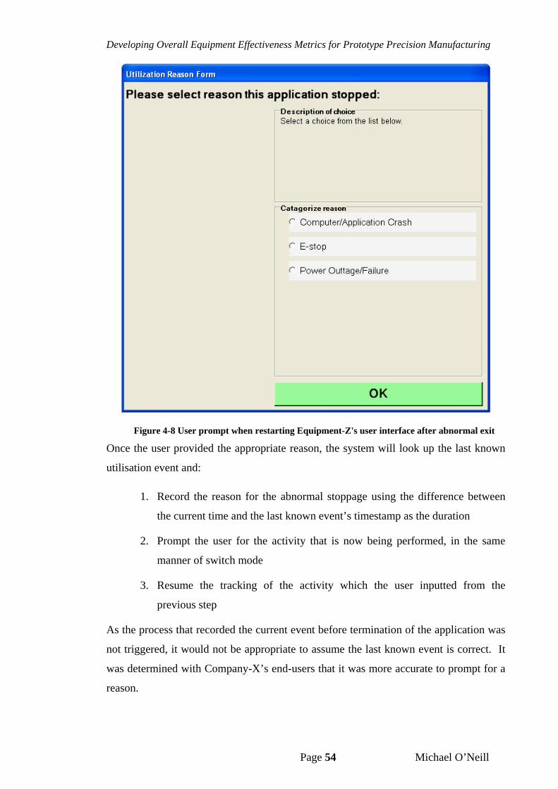
Developing Overall Equipment Effectiveness Metrics for Prototype Precision Manufacturing
Page 54 Michael O’Neill
Figure 4-8 User prompt when restarting Equipment-Z's user interface after abnormal exit
Once the user provided the appropriate reason, the system will look up the last known
utilisation event and:
1. Record the reason for the abnormal stoppage using the difference between
the current time and the last known event’s timestamp as the duration
2. Prompt the user for the activity that is now being performed, in the same
manner of switch mode
3. Resume the tracking of the activity which the user inputted from the
previous step
As the process that recorded the current event before termination of the application was
not triggered, it would not be appropriate to assume the last known event is correct. It
was determined with Company-X’s end-users that it was more accurate to prompt for a
reason.
Developing Overall Equipment Effectiveness Metrics for Prototype Precision Manufacturing
Page 55 Michael O’Neill
4.5.2 Incrementalrecording
In the last example, a situation where Equipment-Z’s interface application is abnormally
and unpredictably terminated, the restoration recording process inferred the timestamp
of the last recorded utilisation event as the start of the abnormal termination event. For
this reason the resolution of the data-capture was an important contributor to the
accuracy of the timestamp.
Consider the following example. The crew of A-shift finishes a day of continuous
production knowing that the line will remain inactive during B-shift as no activities or
crew is scheduled. Following the new business rules, the operator of Equipment-Z
informs it of the Scheduled Down-Time event and leaves the line. The utilisation-
tracking system captures the time of previous event, namely running-time. It knows it
is currently in a Scheduled Down-Time mode, but it will not record this fact until
Equipment-Z is put into a new mode. Ten hours into the twelve hours of Scheduled-
Down-Time, a failure occurs killing all power to the line and instantly terminating
Equipment-Z’s interface application and utilisation tracking. Two hours later the
operators of C-shift arrive on the line to find that power has been restored, but
Equipment-Z needs to be initialised. When the interface application restarts and the
utilisation-tracker attempts to restore itself, the operator informs the system that a power
failure occurs. The system identifies the last known event as “running production”. It
assigns twelve hours to an Unscheduled-Down-Time event (power failure) rather than
ten hours to an Unscheduled-Down-Time event and two hours to an Unscheduled-
Down-Time event.
It should be also be noted that even without the failure, were a manager to query the
database for the utilisation of the line over the last 24 hours at any point during the
Scheduled-Down-Time , the results would not include the fact of the Scheduled-Down-
Time .
For both of these reasons it was decided that the utilisation-tracking system needed to
record the current status after some discrete interval of time where the status did not
change. After reviewing this requirement with end-users it was determined that a
fifteen minute interval was a reasonable resolution of time although it could be changed
in the future. In the failure example above, this resolution would represent the margin
of error in the time assigned to Scheduled Down-Time event (9.75-10 hours) and the
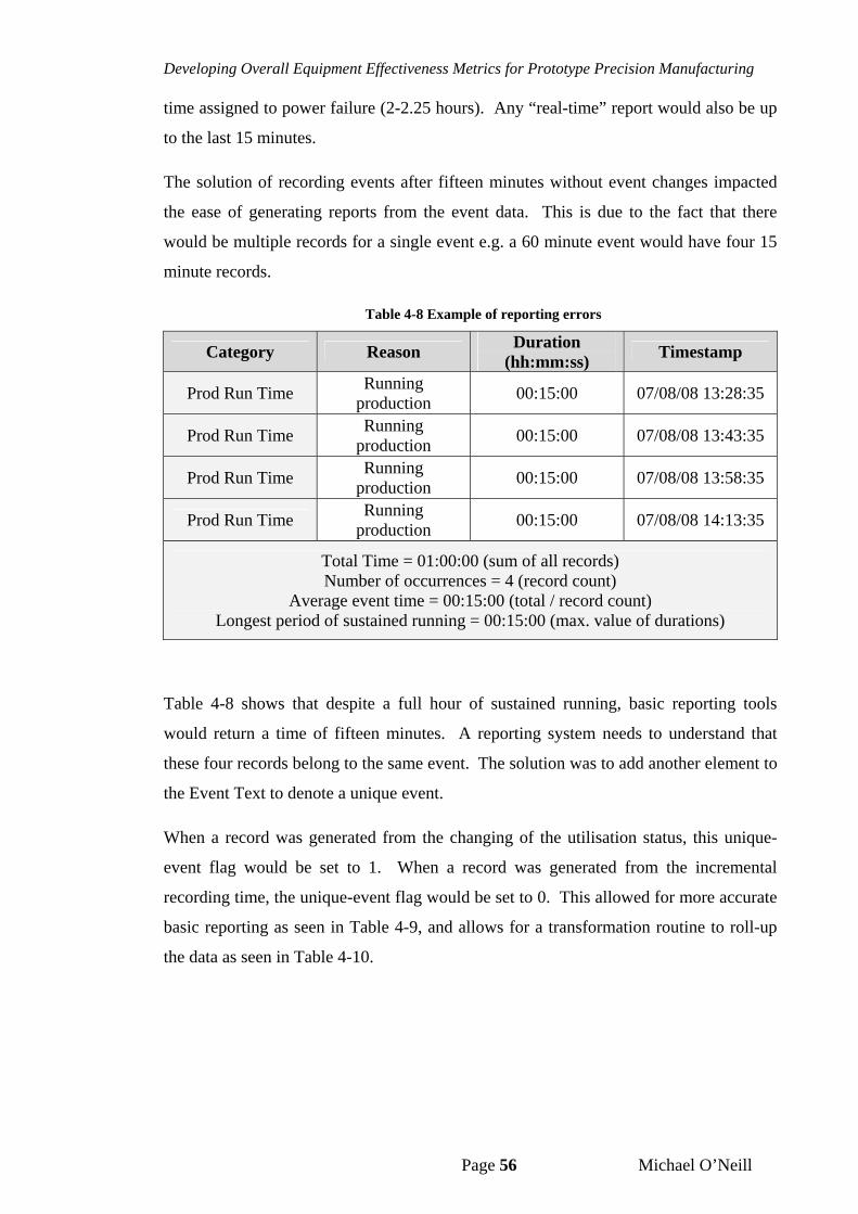
Developing Overall Equipment Effectiveness Metrics for Prototype Precision Manufacturing
Page 56 Michael O’Neill
time assigned to power failure (2-2.25 hours). Any “real-time” report would also be up
to the last 15 minutes.
The solution of recording events after fifteen minutes without event changes impacted
the ease of generating reports from the event data. This is due to the fact that there
would be multiple records for a single event e.g. a 60 minute event would have four 15
minute records.
Table 4-8 Example of reporting errors
Category Reason Duration
(hh:mm:ss) Timestamp
Prod Run Time Running
production 00:15:00 07/08/08 13:28:35
Prod Run Time Running
production 00:15:00 07/08/08 13:43:35
Prod Run Time Running
production 00:15:00 07/08/08 13:58:35
Prod Run Time Running
production 00:15:00 07/08/08 14:13:35
Total Time = 01:00:00 (sum of all records) Number of occurrences = 4 (record count)
Average event time = 00:15:00 (total / record count) Longest period of sustained running = 00:15:00 (max. value of durations)
Table 4-8 shows that despite a full hour of sustained running, basic reporting tools
would return a time of fifteen minutes. A reporting system needs to understand that
these four records belong to the same event. The solution was to add another element to
the Event Text to denote a unique event.
When a record was generated from the changing of the utilisation status, this unique-
event flag would be set to 1. When a record was generated from the incremental
recording time, the unique-event flag would be set to 0. This allowed for more accurate
basic reporting as seen in Table 4-9, and allows for a transformation routine to roll-up
the data as seen in Table 4-10.
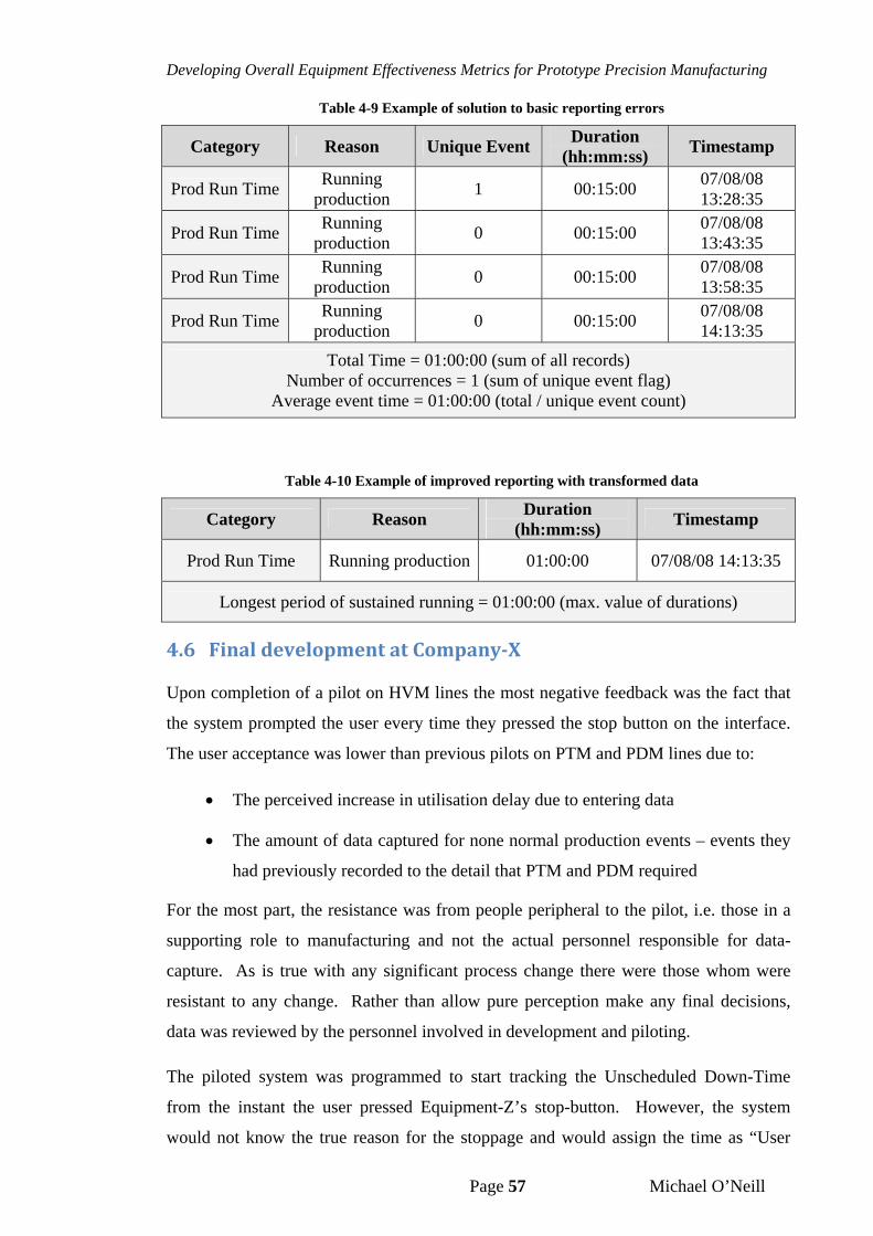
Developing Overall Equipment Effectiveness Metrics for Prototype Precision Manufacturing
Page 57 Michael O’Neill
Table 4-9 Example of solution to basic reporting errors
Category Reason Unique Event Duration
(hh:mm:ss) Timestamp
Prod Run Time Running
production 1 00:15:00
07/08/08 13:28:35
Prod Run Time Running
production 0 00:15:00
07/08/08 13:43:35
Prod Run Time Running
production 0 00:15:00
07/08/08 13:58:35
Prod Run Time Running
production 0 00:15:00
07/08/08 14:13:35
Total Time = 01:00:00 (sum of all records) Number of occurrences = 1 (sum of unique event flag)
Average event time = 01:00:00 (total / unique event count)
Table 4-10 Example of improved reporting with transformed data
Category Reason Duration
(hh:mm:ss) Timestamp
Prod Run Time Running production 01:00:00 07/08/08 14:13:35
Longest period of sustained running = 01:00:00 (max. value of durations)
4.6 FinaldevelopmentatCompany‐X
Upon completion of a pilot on HVM lines the most negative feedback was the fact that
the system prompted the user every time they pressed the stop button on the interface.
The user acceptance was lower than previous pilots on PTM and PDM lines due to:
The perceived increase in utilisation delay due to entering data
The amount of data captured for none normal production events – events they
had previously recorded to the detail that PTM and PDM required
For the most part, the resistance was from people peripheral to the pilot, i.e. those in a
supporting role to manufacturing and not the actual personnel responsible for data-
capture. As is true with any significant process change there were those whom were
resistant to any change. Rather than allow pure perception make any final decisions,
data was reviewed by the personnel involved in development and piloting.
The piloted system was programmed to start tracking the Unscheduled Down-Time
from the instant the user pressed Equipment-Z’s stop-button. However, the system
would not know the true reason for the stoppage and would assign the time as “User
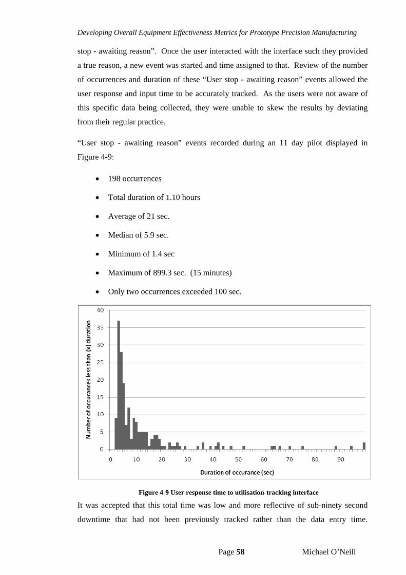
Developing Overall Equipment Effectiveness Metrics for Prototype Precision Manufacturing
Page 58 Michael O’Neill
stop - awaiting reason”. Once the user interacted with the interface such they provided
a true reason, a new event was started and time assigned to that. Review of the number
of occurrences and duration of these “User stop - awaiting reason” events allowed the
user response and input time to be accurately tracked. As the users were not aware of
this specific data being collected, they were unable to skew the results by deviating
from their regular practice.
“User stop - awaiting reason” events recorded during an 11 day pilot displayed in
Figure 4-9:
198 occurrences
Total duration of 1.10 hours
Average of 21 sec.
Median of 5.9 sec.
Minimum of 1.4 sec
Maximum of 899.3 sec. (15 minutes)
Only two occurrences exceeded 100 sec.
Figure 4-9 User response time to utilisation-tracking interface
It was accepted that this total time was low and more reflective of sub-ninety second
downtime that had not been previously tracked rather than the data entry time.
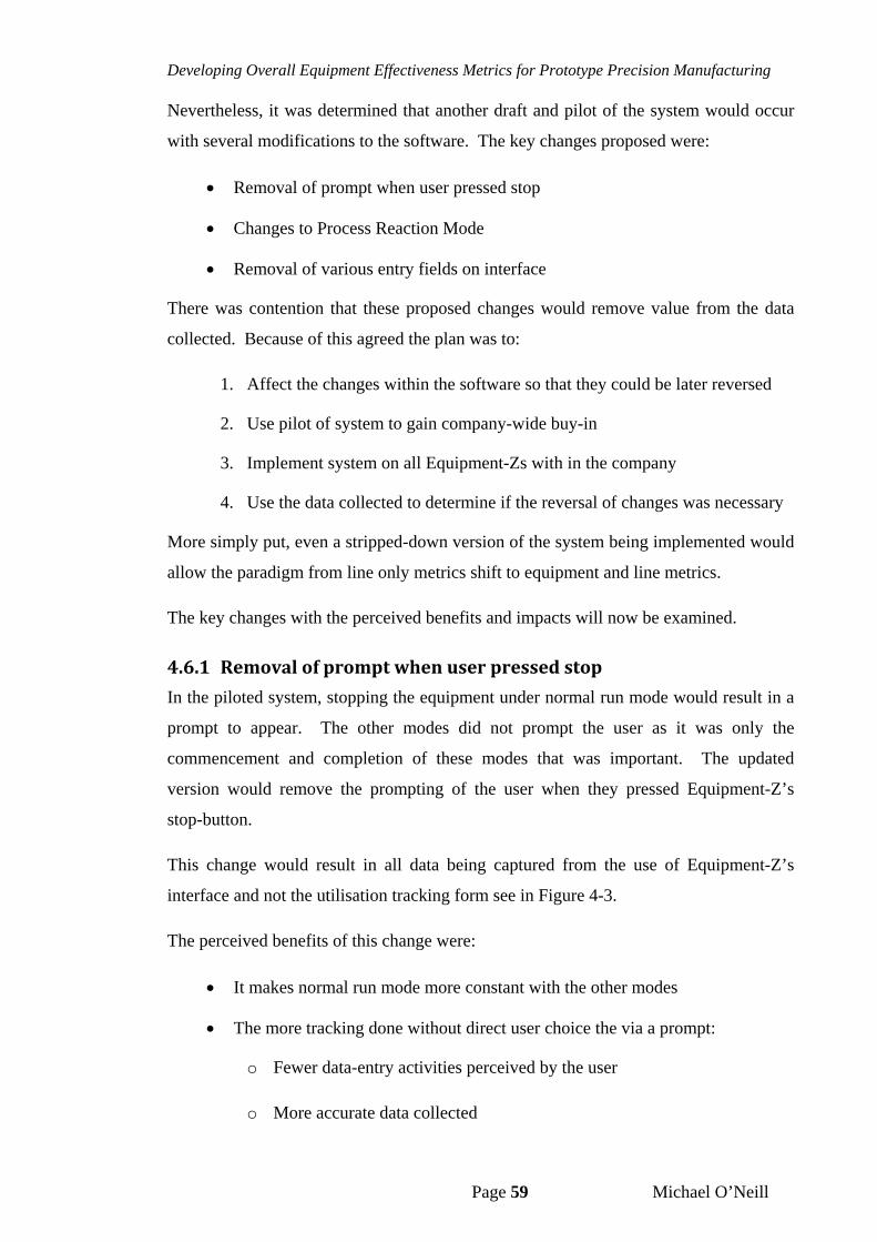
Developing Overall Equipment Effectiveness Metrics for Prototype Precision Manufacturing
Page 59 Michael O’Neill
Nevertheless, it was determined that another draft and pilot of the system would occur
with several modifications to the software. The key changes proposed were:
Removal of prompt when user pressed stop
Changes to Process Reaction Mode
Removal of various entry fields on interface
There was contention that these proposed changes would remove value from the data
collected. Because of this agreed the plan was to:
1. Affect the changes within the software so that they could be later reversed
2. Use pilot of system to gain company-wide buy-in
3. Implement system on all Equipment-Zs with in the company
4. Use the data collected to determine if the reversal of changes was necessary
More simply put, even a stripped-down version of the system being implemented would
allow the paradigm from line only metrics shift to equipment and line metrics.
The key changes with the perceived benefits and impacts will now be examined.
4.6.1 Removalofpromptwhenuserpressedstop
In the piloted system, stopping the equipment under normal run mode would result in a
prompt to appear. The other modes did not prompt the user as it was only the
commencement and completion of these modes that was important. The updated
version would remove the prompting of the user when they pressed Equipment-Z’s
stop-button.
This change would result in all data being captured from the use of Equipment-Z’s
interface and not the utilisation tracking form see in Figure 4-3.
The perceived benefits of this change were:
It makes normal run mode more constant with the other modes
The more tracking done without direct user choice the via a prompt:
o Fewer data-entry activities perceived by the user
o More accurate data collected
Developing Overall Equipment Effectiveness Metrics for Prototype Precision Manufacturing
Page 60 Michael O’Neill
The perceived impacts were:
Response times would be slower as the prompting created a sense of urgency
Switching modes would take longer as users would now have to press the
‘switch mode’ button to display an equivalent prompt
As previously stated, these perceptions could be proven or disproved by running the
system with this change and without this change in the same manufacturing lines, with
the same personnel for the same duration of time. A side-by-side data analysis would
conclude which method had the most delay before data-entry.
4.6.2 ChangestoProcessReactionMode
Originally Process Reaction Mode was programmed such that it would be used when
the operator was required to make a short, single stop to address an issue. This assumed
that upon resumption of running product, the equipment was back to running Normal
Run Mode. All time in Process Reaction Mode was classified as ‘Unscheduled Down
Time”. This made sense in the PTM and PDM lines where Troubleshooting Mode
would be used for more significant stops.
The situation within the HVM plants proved not to be the same. Troubleshooting mode
was deliberately avoided as it had the consequence of rejecting all units processed while
the Equipment-Z was in that mode. The need to react to process issues while lower in
occurrence in HVM often required a short interval of time with frequent stopping and
restarting of the equipment. The piloted system proved cumbersome as the user had to
frequently switch mode to unlock the additional functions.
With these two sets of requirements known, the various end-users collaborated to find a
better alternative to meet all requirements:
Pressing the ‘Start’ button in Process Reaction Mode would no longer
automatically switch the equipment into Normal Run Mode.
Switching to Normal Run Mode would occur in the following manner:
o User pressed ‘Switch Mode’ button and selects Normal Run Mode
o Equipment processed 120 units without stopping
Meeting this criteria would automatically switch the equipment
into Normal Run Mode
Developing Overall Equipment Effectiveness Metrics for Prototype Precision Manufacturing
Page 61 Michael O’Neill
Equipment software would make the change with no prompting
or warning to the user
User would clearly see the change due to the colour-coding of the
modes
Utilisation events would no longer be classified solely as “Unscheduled Down
Time”, rather it would be treated similarly similar to NRM:
o While the equipment was running: “Prod Run Time”
o While the equipment was idle: “Prod Idle Time” with automatic
assignment
o While the equipment was stopped: “Unscheduled Down Time” with the
reason provided by the user when they initially switched to Process
Reaction Mode
These changes were seen as improving the categorisation of the utilisation data. Also
there was no perceived impact to user acceptance of given the collaborative efforts of
the various end-users to determine these changes.
4.6.3 Removalofvariousentryfieldsoninterface
In initial development, considerable thought was put into determining what cause-
information would need to be coupled with any event captured to give it context for
decision-making. An example is the drop-down fields provided when the user is
switching into Process Reaction Mode as is seen in Figure 4-10 & Figure 4-11.
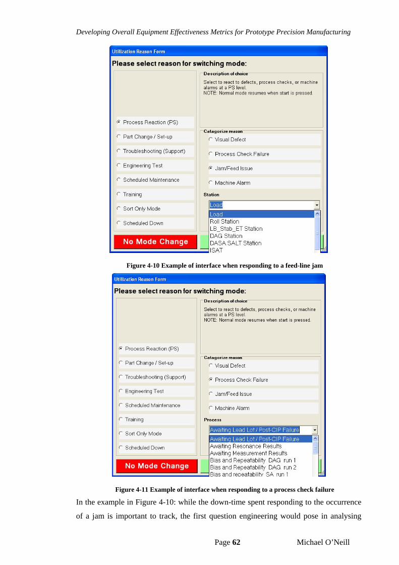
Developing Overall Equipment Effectiveness Metrics for Prototype Precision Manufacturing
Page 62 Michael O’Neill
Figure 4-10 Example of interface when responding to a feed-line jam
Figure 4-11 Example of interface when responding to a process check failure
In the example in Figure 4-10: while the down-time spent responding to the occurrence
of a jam is important to track, the first question engineering would pose in analysing
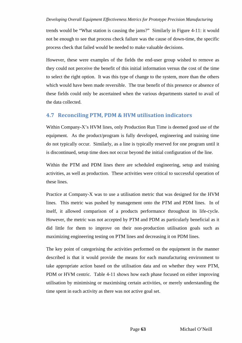
Developing Overall Equipment Effectiveness Metrics for Prototype Precision Manufacturing
Page 63 Michael O’Neill
trends would be “What station is causing the jams?” Similarly in Figure 4-11: it would
not be enough to see that process check failure was the cause of down-time, the specific
process check that failed would be needed to make valuable decisions.
However, these were examples of the fields the end-user group wished to remove as
they could not perceive the benefit of this initial information versus the cost of the time
to select the right option. It was this type of change to the system, more than the others
which would have been made reversible. The true benefit of this presence or absence of
these fields could only be ascertained when the various departments started to avail of
the data collected.
4.7 ReconcilingPTM,PDM&HVMutilisationindicators
Within Company-X’s HVM lines, only Production Run Time is deemed good use of the
equipment. As the product/program is fully developed, engineering and training time
do not typically occur. Similarly, as a line is typically reserved for one program until it
is discontinued, setup time does not occur beyond the initial configuration of the line.
Within the PTM and PDM lines there are scheduled engineering, setup and training
activities, as well as production. These activities were critical to successful operation of
these lines.
Practice at Company-X was to use a utilisation metric that was designed for the HVM
lines. This metric was pushed by management onto the PTM and PDM lines. In of
itself, it allowed comparison of a products performance throughout its life-cycle.
However, the metric was not accepted by PTM and PDM as particularly beneficial as it
did little for them to improve on their non-production utilisation goals such as
maximizing engineering testing on PTM lines and decreasing it on PDM lines.
The key point of categorising the activities performed on the equipment in the manner
described is that it would provide the means for each manufacturing environment to
take appropriate action based on the utilisation data and on whether they were PTM,
PDM or HVM centric. Table 4-11 shows how each phase focused on either improving
utilisation by minimising or maximising certain activities, or merely understanding the
time spent in each activity as there was not active goal set.
Developing Overall Equipment Effectiveness Metrics for Prototype Precision Manufacturing
Page 64 Michael O’Neill
Table 4-11 Activity goals per phase of program life-cycle
MODE PTM PDM HVM
Production Run Time Understand Maximise Maximise
Production Idle Time Understand Understand Minimise
Unscheduled Down Time Understand Minimise Minimise
Scheduled Setup Time Minimise Understand Minimise
Engineering Test Time Maximise Minimise Minimise
Scheduled Maintenance Time Understand Understand Understand
Scheduled Training Time Understand Understand Understand
Scheduled Down Time Minimise Minimise Minimise
When users understood how each phase looked at each activity, they began to rethink
and seem to accept a different utilisation formula than one that outright penalised
engineering, setup and training activity. In HVM, these were effectively treated as
Unscheduled-Down-Time, and therefore included as Available-Time, TAVAIL. PTM and
PDM management wanted to effectively treat these as running time as they considered
this positive utilisation.
The emerging compromise was to return to the industry definitions used for utilisation
and treat these scheduled activities as Scheduled Down-Time. The allowed Company-
X’s utilisation metric to focus on utilisation with respect to producing units of product
while not penalising required development activities as the Scheduled-Down-Time is
removed from calendar-time to deduce Available-Time per Equation 8.
4.8 ChapterSummary
The system was developed to explicitly capture and categorise all time events into
production (running, idle, unscheduled down) time and non-production scheduled
(setup, engineering, maintenance) time. Wherever possible the equipment’s computer-
controller performed these activities automatically. When it was necessary, the system
would force the equipment operator to provide the minimally needed information. With
the utilisation indicator portion designed, development moved to efficiency and yield
indicators.
Developing Overall Equipment Effectiveness Metrics for Prototype Precision Manufacturing
Page 65 Michael O’Neill
5 DevelopmentofEfficiency&YieldCapture
5.1 EfficiencyCapture
The efficiency indicators, Equations 15 and 18, require the capture of two out of the
four unique factors:
The fastest time the equipment is rated or bench-marked to be able to process a
unit; known as rated cycle-time, CTRated
The actual time spent by the equipment to process a unit; known as actual
cycle-time, CTActual
The greatest number of units the equipment is rated or bench-marked to be
able to process a in fixed time period, typically expressed in terms of an hour;
known as rated output-rate, UPHRated
The actual number of units the equipment processed a in fixed time period,
typically expressed in terms of an hour; known as actual output-rate UPHActual
As explained in Section 2.3, cycle-time can be calculated from output-rate. For this
reason only two of these four factors need to be captured. Each of these factors present
their own data-capture issues which be now be examined.
5.1.1 RatedCycle‐timeandOutput‐rate
Most of Company-X’s equipment consists of various components purchased from
Original Equipment Manufacturers (OEM), and then assembled by Company-X’s
personnel. While the components could well have cycle-times rated and specified by
their OEM, the equipment assembled and tailored by Company-X would not
immediately have a rated cycle-time.
The obvious solution is that Company-X would need to establish its own rating of its
equipment. Company-X does have a rating for its HMV lines but not necessarily the
individual pieces of equipment that comprise the line. Equipment ratings however
could easily be established through historical data.
As was stated for cycle-time, the same is true for output-rate.
Developing Overall Equipment Effectiveness Metrics for Prototype Precision Manufacturing
Page 66 Michael O’Neill
5.1.2 ActualCycle‐time
Automatic cycle-time capture requires the means to capture the time sent processing
each unit individually. This method requires the intelligence of the equipment to
independently capture and record the time when an individual unit enters the equipment
to the time that unit is fully processed and leaves the equipment.
Some months prior to the commencement of this project, a separate effort was
completed for Equipment-Z to capture and record the actual cycle-time. As it had
multiple internal stations and a feed-system which transported each cavity of each
carrier to the each station, the cycle-time tracking system recorded:
The cycle-time of each station per unit
The wait-time for the upstream process to load a carrier into the equipment
The wait-time for the downstream process to unload a carrier from the
equipment
The cycle time of the equipment to move a unit to the next station and process
it – which was a function of:
o Upstream wait-time
o Downstream wait-time
o The parallel processing-times of all the individual stations
As the starting and stopping of times were tied to the PLC controllers of Equipment-Z
the accuracy of these times is not in dispute. What is remarkable is that these times
were used only to improve the cycle-time of Equipment-Z and not used in a manner to
calculate the efficiency of Equipment-Z. One reason was the lack of a benchmarked or
rated cycle-time, which resulted in losses that were not quantifiable, and therefore could
not be categorized.
Another remarkable feature of this cycle-time tracking was the concept of steady-state
and non-steady-state cycle-time. The engineers who designed and implemented this
system understood that the cycle-time would change based on environmental
differences. For example, if the equipment was full i.e. it was processing a full set of
carriers which in turn had units in all cavities, and the upstream and downstream
process were immediately ready to load and unload, then Equipment-Z was deemed to
be in steady-state and all recorded times were categorised as such.
Developing Overall Equipment Effectiveness Metrics for Prototype Precision Manufacturing
Page 67 Michael O’Neill
When Equipment-Z was in non-steady-state, there was the risk that the captured times
would be impacted such that they would not accurately reflect the actual cycle-time of
the equipment. Examples of these impacts were:
Increase in station processing-time as Equipment-Z has to warm up due to
being idle for some time
Decrease in overall processing time as feed-system immediately indexes a
second time as no units were presented to any stations
The engineers using the cycle-time tracking system would filter out the non-steady-state
information and only deem the steady-state information as the true speed of the
equipment.
With respect to OEE, this steady-state cycle-time seems to be a closer reflection of the
actual cycle-time in that is not convoluted with yield and utilisation losses from
upstream or downstream equipment in the same line. The average of the recorded
cycle-times for time-period should be compared to the rated cycle-time to compute the
efficiency indicator.
5.1.3 ActualOutput‐rate
For a given period of time, the capture of the actual output-rate requires the capture of
two factors:
The number of units processed
The duration of processing time
Per the proposed utilisation-tracking system the run time of the equipment, TRun, will be
captured and recorded, which can serve as the duration of processing time. As will be
seen later, the yield-tracking system will count the number of units fed into to the
equipment, uin, which can serve as the number of units processed.
This makes it possible to use the utilisation and yield factors to as efficiency factors,
assuming TRun is in hours:
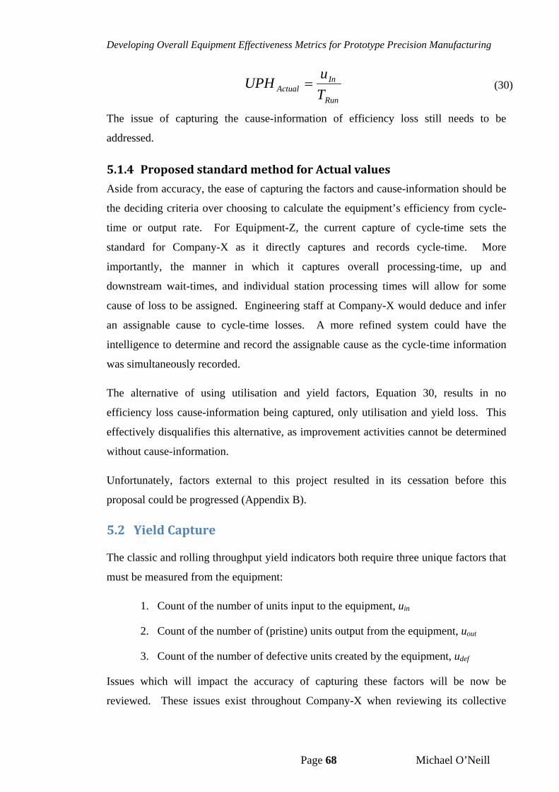
Developing Overall Equipment Effectiveness Metrics for Prototype Precision Manufacturing
Page 68 Michael O’Neill
Run
InActual T
uUPH
(30)
The issue of capturing the cause-information of efficiency loss still needs to be
addressed.
5.1.4 ProposedstandardmethodforActualvalues
Aside from accuracy, the ease of capturing the factors and cause-information should be
the deciding criteria over choosing to calculate the equipment’s efficiency from cycle-
time or output rate. For Equipment-Z, the current capture of cycle-time sets the
standard for Company-X as it directly captures and records cycle-time. More
importantly, the manner in which it captures overall processing-time, up and
downstream wait-times, and individual station processing times will allow for some
cause of loss to be assigned. Engineering staff at Company-X would deduce and infer
an assignable cause to cycle-time losses. A more refined system could have the
intelligence to determine and record the assignable cause as the cycle-time information
was simultaneously recorded.
The alternative of using utilisation and yield factors, Equation 30, results in no
efficiency loss cause-information being captured, only utilisation and yield loss. This
effectively disqualifies this alternative, as improvement activities cannot be determined
without cause-information.
Unfortunately, factors external to this project resulted in its cessation before this
proposal could be progressed (Appendix B).
5.2 YieldCapture
The classic and rolling throughput yield indicators both require three unique factors that
must be measured from the equipment:
1. Count of the number of units input to the equipment, uin
2. Count of the number of (pristine) units output from the equipment, uout
3. Count of the number of defective units created by the equipment, udef
Issues which will impact the accuracy of capturing these factors will be now be
reviewed. These issues exist throughout Company-X when reviewing its collective
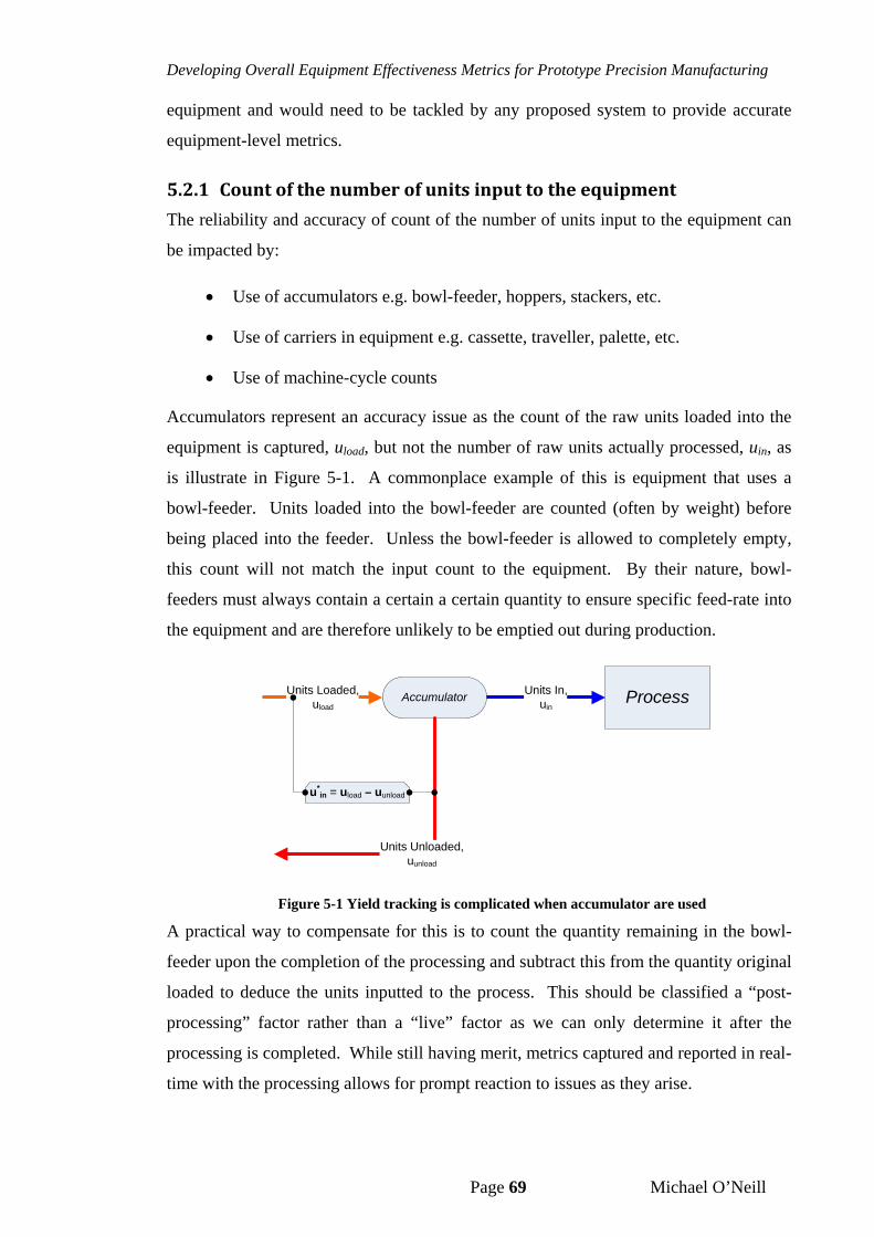
Developing Overall Equipment Effectiveness Metrics for Prototype Precision Manufacturing
Page 69 Michael O’Neill
equipment and would need to be tackled by any proposed system to provide accurate
equipment-level metrics.
5.2.1 Countofthenumberofunitsinputtotheequipment
The reliability and accuracy of count of the number of units input to the equipment can
be impacted by:
Use of accumulators e.g. bowl-feeder, hoppers, stackers, etc.
Use of carriers in equipment e.g. cassette, traveller, palette, etc.
Use of machine-cycle counts
Accumulators represent an accuracy issue as the count of the raw units loaded into the
equipment is captured, uload, but not the number of raw units actually processed, uin, as
is illustrate in Figure 5-1. A commonplace example of this is equipment that uses a
bowl-feeder. Units loaded into the bowl-feeder are counted (often by weight) before
being placed into the feeder. Unless the bowl-feeder is allowed to completely empty,
this count will not match the input count to the equipment. By their nature, bowl-
feeders must always contain a certain a certain quantity to ensure specific feed-rate into
the equipment and are therefore unlikely to be emptied out during production.
ProcessUnits In,uin
AccumulatorUnits Loaded,
uload
Units Unloaded,uunload
u*in = uload – uunload
Figure 5-1 Yield tracking is complicated when accumulator are used
A practical way to compensate for this is to count the quantity remaining in the bowl-
feeder upon the completion of the processing and subtract this from the quantity original
loaded to deduce the units inputted to the process. This should be classified a “post-
processing” factor rather than a “live” factor as we can only determine it after the
processing is completed. While still having merit, metrics captured and reported in real-
time with the processing allows for prompt reaction to issues as they arise.
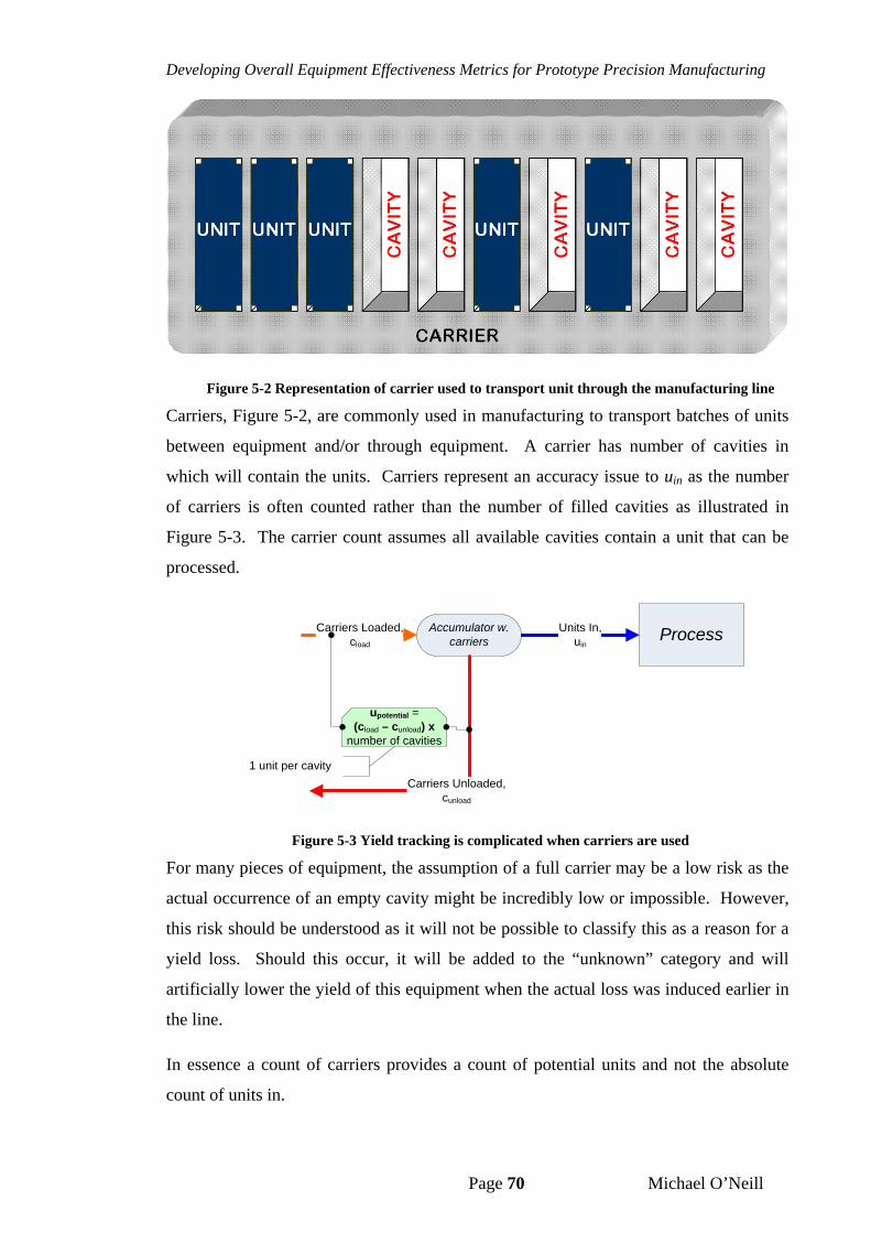
Developing Overall Equipment Effectiveness Metrics for Prototype Precision Manufacturing
Page 70 Michael O’Neill
Figure 5-2 Representation of carrier used to transport unit through the manufacturing line
Carriers, Figure 5-2, are commonly used in manufacturing to transport batches of units
between equipment and/or through equipment. A carrier has number of cavities in
which will contain the units. Carriers represent an accuracy issue to uin as the number
of carriers is often counted rather than the number of filled cavities as illustrated in
Figure 5-3. The carrier count assumes all available cavities contain a unit that can be
processed.
ProcessUnits In,uin
Accumulator w. carriers
Carriers Loaded,cload
Carriers Unloaded,cunload
upotential =(cload – cunload) x
number of cavities
1 unit per cavity
Figure 5-3 Yield tracking is complicated when carriers are used
For many pieces of equipment, the assumption of a full carrier may be a low risk as the
actual occurrence of an empty cavity might be incredibly low or impossible. However,
this risk should be understood as it will not be possible to classify this as a reason for a
yield loss. Should this occur, it will be added to the “unknown” category and will
artificially lower the yield of this equipment when the actual loss was induced earlier in
the line.
In essence a count of carriers provides a count of potential units and not the absolute
count of units in.
Developing Overall Equipment Effectiveness Metrics for Prototype Precision Manufacturing
Page 71 Michael O’Neill
cavitiesCarrieru InPotential (1)
While also ensuring the accuracy of the yield of this equipment being able to discern the
units actually input to the equipment provides the means to validate the yields of
previous equipment in the line.
Defective units on a carrier are similar to empty cavities on the carrier in that there is
not a unit that can be processed. Some of Company-X’s equipment, including
Equipment-Z, has the ability to identify and skip the processing of these defective units.
This is ideal as they should not counted either as units input to the equipment, output
from the equipment or defective due to the equipment. Thus uPotential is not used as an
estimate of uIn, but rather it is used as an independent factor.
Use of a machine-cycle count in the place of a units inputted count present similar
accuracy issues as carriers. If the equipment cycles irrespective of available unit and/or
a non-defective unit then this clearly cannot represent the quantity of units to be
processed.
To summarize, the most accurate count of units fed into the equipment will differentiate
units that are both non-defective from previous equipment in the line and are actively
received/processed by the equipment. This can be achieved by placing a sensor
(proximity sensor, IR sensor, etc) to detect units present at the first point of work within
the equipment. If it is possible for defective units to be present, a more difficult
problem is presented. The equipment needs some means to determine defective units
from pristine units. The unit needs some mark, identifier or feature to signal it as
defective. The equipment needs to some means to sense this “signal”.
Examples of signalling and sensing defective units include:
Vision system to read a mark (ink spot, lasered dot, missing tab) from a region
of the unit used to communicate pristine condition
o Upstream equipment (or operator) must mark the inspected region once
unit is found to be defective.
Barcode scanner to read the unit’s barcode identifier and query a database
which has the unit’s pristine or defective condition recorded
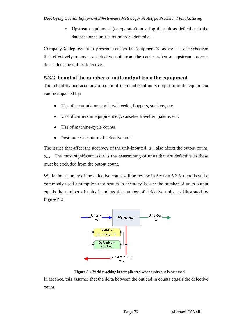
Developing Overall Equipment Effectiveness Metrics for Prototype Precision Manufacturing
Page 72 Michael O’Neill
o Upstream equipment (or operator) must log the unit as defective in the
database once unit is found to be defective.
Company-X deploys “unit present” sensors in Equipment-Z, as well as a mechanism
that effectively removes a defective unit from the carrier when an upstream process
determines the unit is defective.
5.2.2 Countofthenumberofunitsoutputfromtheequipment
The reliability and accuracy of count of the number of units output from the equipment
can be impacted by:
Use of accumulators e.g. bowl-feeder, hoppers, stackers, etc.
Use of carriers in equipment e.g. cassette, traveller, palette, etc.
Use of machine-cycle counts
Post process capture of defective units
The issues that affect the accuracy of the unit-inputted, uin, also affect the output count,
uout. The most significant issue is the determining of units that are defective as these
must be excluded from the output count.
While the accuracy of the defective count will be review in Section 5.2.3, there is still a
commonly used assumption that results in accuracy issues: the number of units output
equals the number of units in minus the number of defective units, as illustrated by
Figure 5-4.
Figure 5-4 Yield tracking is complicated when units out is assumed
In essence, this assumes that the delta between the out and in counts equals the defective
count.
Developing Overall Equipment Effectiveness Metrics for Prototype Precision Manufacturing
Page 73 Michael O’Neill
uuu OutIn (31)
uuDef (32)
DefInOut uuu (33)
On paper this makes sense, but in practical application this can present a problem. It is
important to consider what can be considered a defective unit. A defective unit should
be one that has a known and documented non-conformance. Therefore a unit can only
be considered defective if there is categorisation of defect data associated with it.
Within Company-X there is equipment where it is possible for units to fall from the
feed-line. This lost product was not classed as defective and it can go unaccounted for
during a manufacturing order. In this example, it is easy to see how there was a
difference between the quantities expected downstream and those actually received.
These differences are problematic as there is not a clear assignable cause captured in
real-time. A post-build investigation must occur to determine and record the cause or
yield loss.
uuDef (34)
Explicitly counting units out from equipment independently of the defective units
allows the distinction between the in-out delta and the defective count. This allows any
post-build investigation to focus at the specific equipment rather than having to first
troubleshoot all the upstream equipment to determine the source. Additionally, seeing
this distinction in real-time will provide those closest to the equipment the opportunity
of identifying the source of the discrepancy and possibly correct it before the processing
is completed.
A cost-benefit analysis may determine for a specific application that the sensing of all
three factors is not appropriate. Equipment-Z indeed has a unit-out sensor. When a unit
expected to exit the equipment fails to be present, Equipment-Z’s programming will
alarm and stop the line. To resume the line, the operator is forced to classify the loss,
and as such this loss is recorded. This methodology makes Equipment-Z’s unit counts
the most accurate in Company-X, effectively ensuring Equation 32 is always true.
Developing Overall Equipment Effectiveness Metrics for Prototype Precision Manufacturing
Page 74 Michael O’Neill
5.2.3 Countofthenumberofdefectiveunitscreatedbytheequipment
The reliability and accuracy of count of the number of defective units created by the
equipment can be impacted by:
Post-process capture of defective units
Ability to remove units from equipment without disposition
As explained in the previous section, it is important to distinguish defective units as
having cause-information, i.e. specifically documented non-conformance. An accurate
count of defective units is dependant on using the systems in place to identify and
document the defective units created by the equipment.
Very few, if any, equipment has built-in capability to test and identify every possible
defect that can be induced by the equipment. For example, equipment that connects a
resistor to a circuit-board may test the connectivity of the resistor and the quality of the
solder joints used, but will it consider the edge of the circuit board for abrasions due to a
burr on the clamping fixture holding the board in place for processing?
Testing, measuring and inspecting for every possible defect at every piece of equipment
is costly and impractical. It is a reality of manufacturing that issues will be identified
after they occur and it is possible this identification will occur downstream of the
equipment where it occurs. It is for this reason Company-X utilises dedicated
inspection processes. These processes are defined at appropriate points on the line to
visually inspect for attribute defects/conformance and measure for variable or
functionality defects/conformance.
Rather than discuss and debate how to make these inspection processes effective, this
work focuses on how to best create the factor and cause data. There are two strategies
commonly deployed to handle this circumstance:
1. Both factor and cause are assigned to the “source” equipment determined to
cause the defect and not the inspection process
A. The outputted unit and defective unit counts for the source equipment are
retroactively changed.
B. Equipment Pareto shows loss
2. The factor is assigned to the inspection process
Developing Overall Equipment Effectiveness Metrics for Prototype Precision Manufacturing
Page 75 Michael O’Neill
A. Being part of the line, the detected loss is ultimately accounted for
B. The cause data is used in a Grand Pareto and not equipment’s Pareto
An argument can be made for the assigning of data to the source of the incident rather
than the location it was discovered, as it would more clearly represent the productivity
of the specific equipment. However there is a more critical circumstance to guide the
decision: when do we want someone to respond to this yield loss?
A real-time capture system is truly beneficial as it presents information to those in the
position to make an immediate improvement to the equipment. Whichever strategy is
chosen, only building a mechanism to empower operators to make improvements during
the processing will improve the final outcome of the build.
Whether the inspection is built-in to the equipment or accomplished via a separate
inspection process/equipment, the biggest root-cause of defect inaccuracies is the lack
of a disposition i.e. requiring the defect to be determined, classified and recorded. Any
system needs to account for and assign cause to every unit that is not output from the
equipment.
As discussed earlier, Company-X’s current disposition practices are very disconnected
from regular production practices. In fact, they are run counter to each other. Any tool
that requires even a perceived loss in productivity in order to record the cause the
reasons for a loss of productivity will be ill-received by the operators tasked with
maintaining productivity. If the disposition practice provides the ability for the operator
to, in their mind, avoid further impact to productivity by skipping the disposition of
yield defects, some will undoubtedly avail of it.
Returning to the example in Section 5.2.2 where units could fall off the feed-line. A
practice needs to be established to ensure the appropriate disposition of these units.
This disposition may involve scrapping the units, or the reworking, testing and returning
of the units to the appropriate equipment on the line. Regardless of the outcome of the
disposition, these units have not completed the regular equipment and the productivity
factors should reflect this.
Developing Overall Equipment Effectiveness Metrics for Prototype Precision Manufacturing
Page 76 Michael O’Neill
5.2.4 RecommendedYieldCaptureSystem
While there are certainly cases where two out of the three yield factors can be used, and
the third one inferred, for all the reasons explained in the previous sections this is not
recommended.
Whilst potentially being the more difficult system to implement, the system that
provides the simplest, clearest factors is one that independently counts for a given piece
of equipment:
1. The good units actually received by the equipment’s value-added process
2. The good units actually output by the equipment
3. The units rendered defective by equipment as and categorised as such
These factors will function no matter how complex the feed-process to the equipment
might be in terms of having accumulators and/or carriers. They provide the means to
ensure that the difference between the count of units fed to the equipment less those
output from the machine matches the count of defective unit, Equation 31 & Equation
34. They also provide the means to ensure that the count of units fed from one piece of
equipment on the line matches the count of units fed into the line’s next piece of
equipment.
Any difference in these values will highlight some inability of the system to accurately
count the units. This should trigger investigation as some as yet unforeseen source of
loss has occurred. Therefore being able to compare the factors can validate the integrity
of the factors and the system.
The further a system must deviate from this model, the more convoluted the factor and
cause information becomes as approximations for these three factors must be used.
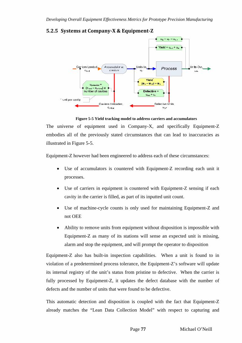
Developing Overall Equipment Effectiveness Metrics for Prototype Precision Manufacturing
Page 77 Michael O’Neill
5.2.5 SystemsatCompany‐X&Equipment‐Z
Figure 5-5 Yield tracking model to address carriers and accumulators
The universe of equipment used in Company-X, and specifically Equipment-Z
embodies all of the previously stated circumstances that can lead to inaccuracies as
illustrated in Figure 5-5.
Equipment-Z however had been engineered to address each of these circumstances:
Use of accumulators is countered with Equipment-Z recording each unit it
processes.
Use of carriers in equipment is countered with Equipment-Z sensing if each
cavity in the carrier is filled, as part of its inputted unit count.
Use of machine-cycle counts is only used for maintaining Equipment-Z and
not OEE
Ability to remove units from equipment without disposition is impossible with
Equipment-Z as many of its stations will sense an expected unit is missing,
alarm and stop the equipment, and will prompt the operator to disposition
Equipment-Z also has built-in inspection capabilities. When a unit is found to in
violation of a predetermined process tolerance, the Equipment-Z’s software will update
its internal registry of the unit’s status from pristine to defective. When the carrier is
fully processed by Equipment-Z, it updates the defect database with the number of
defects and the number of units that were found to be defective.
This automatic detection and disposition is coupled with the fact that Equipment-Z
already matches the “Lean Data Collection Model” with respect to capturing and
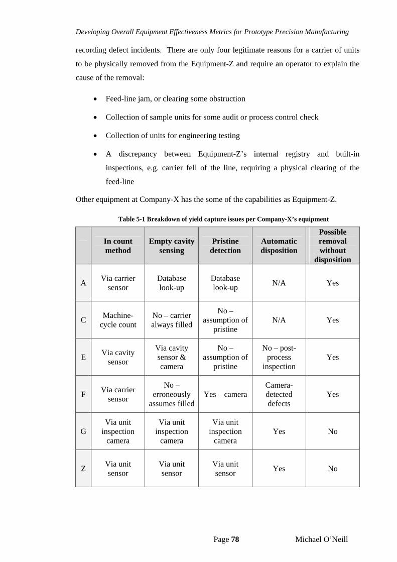
Developing Overall Equipment Effectiveness Metrics for Prototype Precision Manufacturing
Page 78 Michael O’Neill
recording defect incidents. There are only four legitimate reasons for a carrier of units
to be physically removed from the Equipment-Z and require an operator to explain the
cause of the removal:
Feed-line jam, or clearing some obstruction
Collection of sample units for some audit or process control check
Collection of units for engineering testing
A discrepancy between Equipment-Z’s internal registry and built-in
inspections, e.g. carrier fell of the line, requiring a physical clearing of the
feed-line
Other equipment at Company-X has the some of the capabilities as Equipment-Z.
Table 5-1 Breakdown of yield capture issues per Company-X’s equipment
In count method
Empty cavity sensing
Pristine detection
Automatic disposition
Possible removal without
disposition
A Via carrier
sensor Database look-up
Database look-up
N/A Yes
C Machine-
cycle count No – carrier always filled
No – assumption of
pristine N/A Yes
E Via cavity
sensor
Via cavity sensor & camera
No – assumption of
pristine
No – post-process
inspection Yes
F Via carrier
sensor
No – erroneously
assumes filledYes – camera
Camera-detected defects
Yes
G Via unit
inspection camera
Via unit inspection
camera
Via unit inspection
camera Yes No
Z Via unit sensor
Via unit sensor
Via unit sensor
Yes No
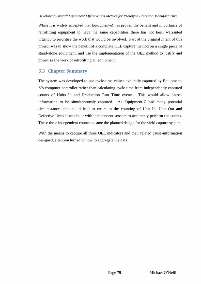
Developing Overall Equipment Effectiveness Metrics for Prototype Precision Manufacturing
Page 79 Michael O’Neill
While it is widely accepted that Equipment-Z has proven the benefit and importance of
retrofitting equipment to have the same capabilities there has not been warranted
urgency to prioritise the work that would be involved. Part of the original intent of this
project was to show the benefit of a complete OEE capture method on a single piece of
stand-alone equipment, and use the implementation of the OEE method to justify and
prioritize the work of retrofitting all equipment.
5.3 ChapterSummary
The system was developed to use cycle-time values explicitly captured by Equipment-
Z’s computer-controller rather than calculating cycle-time from independently captured
counts of Units In and Production Run Time events. This would allow cause-
information to be simultaneously captured. As Equipment-Z had many potential
circumstances that could lead to errors in the counting of Unit In, Unit Out and
Defective Units it was built with independent sensors to accurately perform the counts.
These three independent counts became the planned design for the yield capture system.
With the means to capture all three OEE indicators and their related cause-information
designed, attention turned to how to aggregate the data.
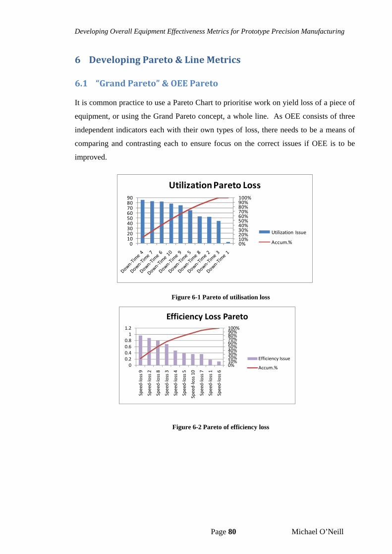
Developing Overall Equipment Effectiveness Metrics for Prototype Precision Manufacturing
Page 80 Michael O’Neill
6 DevelopingPareto&LineMetrics
6.1 “GrandPareto”&OEEPareto
It is common practice to use a Pareto Chart to prioritise work on yield loss of a piece of
equipment, or using the Grand Pareto concept, a whole line. As OEE consists of three
independent indicators each with their own types of loss, there needs to be a means of
comparing and contrasting each to ensure focus on the correct issues if OEE is to be
improved.
0%10%20%30%40%50%60%70%80%90%100%
0102030405060708090
Utilization Pareto Loss
Utilization Issue
Accum.%
Figure 6-1 Pareto of utilisation loss
0%10%20%30%40%50%60%70%80%90%100%
00.20.40.60.81
1.2
Speed‐loss 9
Speed‐loss 2
Speed‐loss 8
Speed‐loss 3
Speed‐loss 4
Speed‐loss 5
Speed‐loss 10
Speed‐loss 7
Speed‐loss 1
Speed‐loss 6
Efficiency Loss Pareto
Efficiency Issue
Accum.%
Figure 6-2 Pareto of efficiency loss
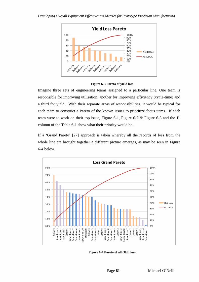
Developing Overall Equipment Effectiveness Metrics for Prototype Precision Manufacturing
Page 81 Michael O’Neill
0%10%20%30%40%50%60%70%80%90%100%
0
20
40
60
80
100
Yield Loss Pareto
Yield Issue
Accum.%
Figure 6-3 Pareto of yield loss
Imagine three sets of engineering teams assigned to a particular line. One team is
responsible for improving utilisation, another for improving efficiency (cycle-time) and
a third for yield. With their separate areas of responsibilities, it would be typical for
each team to construct a Pareto of the known issues to prioritize focus items. If each
team were to work on their top issue, Figure 6-1, Figure 6-2 & Figure 6-3 and the 1st
column of the Table 6-1 show what their priority would be.
If a ‘Grand Pareto’ [27] approach is taken whereby all the records of loss from the
whole line are brought together a different picture emerges, as may be seen in Figure
6-4 below.
0%
10%
20%
30%
40%
50%
60%
70%
80%
90%
100%
0.0%
1.0%
2.0%
3.0%
4.0%
5.0%
6.0%
7.0%
8.0%
Defect 9
Speed‐loss 9
Speed‐loss 2
Speed‐loss 8
Defect 6
Down‐Time 4
Down‐Time 7
Down‐Time 6
Speed‐loss 3
Down‐Time 10
Defect 10
Defect 3
Down‐Time 9
Down‐Time 5
Defect 1
Defect 8
Speed‐loss 4
Down‐Time 8
Down‐Time 2
Speed‐loss 5
Defect 2
Down‐Time 3
Speed‐loss 10
Speed‐loss 7
Defect 7
Defect 5
Defect 4
Speed‐loss 1
Speed‐loss 6
Down‐Time 1
Loss Grand Pareto
OEE Loss
Accum.%
Figure 6-4 Pareto of all OEE loss
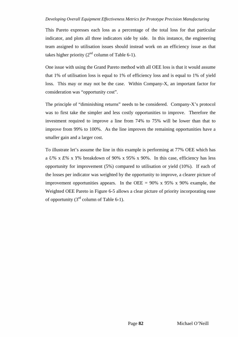
Developing Overall Equipment Effectiveness Metrics for Prototype Precision Manufacturing
Page 82 Michael O’Neill
This Pareto expresses each loss as a percentage of the total loss for that particular
indicator, and plots all three indicators side by side. In this instance, the engineering
team assigned to utilisation issues should instead work on an efficiency issue as that
takes higher priority (2nd column of Table 6-1).
One issue with using the Grand Pareto method with all OEE loss is that it would assume
that 1% of utilisation loss is equal to 1% of efficiency loss and is equal to 1% of yield
loss. This may or may not be the case. Within Company-X, an important factor for
consideration was “opportunity cost”.
The principle of “diminishing returns” needs to be considered. Company-X’s protocol
was to first take the simpler and less costly opportunities to improve. Therefore the
investment required to improve a line from 74% to 75% will be lower than that to
improve from 99% to 100%. As the line improves the remaining opportunities have a
smaller gain and a larger cost.
To illustrate let’s assume the line in this example is performing at 77% OEE which has
a U% x E% x Y% breakdown of 90% x 95% x 90%. In this case, efficiency has less
opportunity for improvement (5%) compared to utilisation or yield (10%). If each of
the losses per indicator was weighted by the opportunity to improve, a clearer picture of
improvement opportunities appears. In the OEE = 90% x 95% x 90% example, the
Weighted OEE Pareto in Figure 6-5 allows a clear picture of priority incorporating ease
of opportunity (3rd column of Table 6-1).
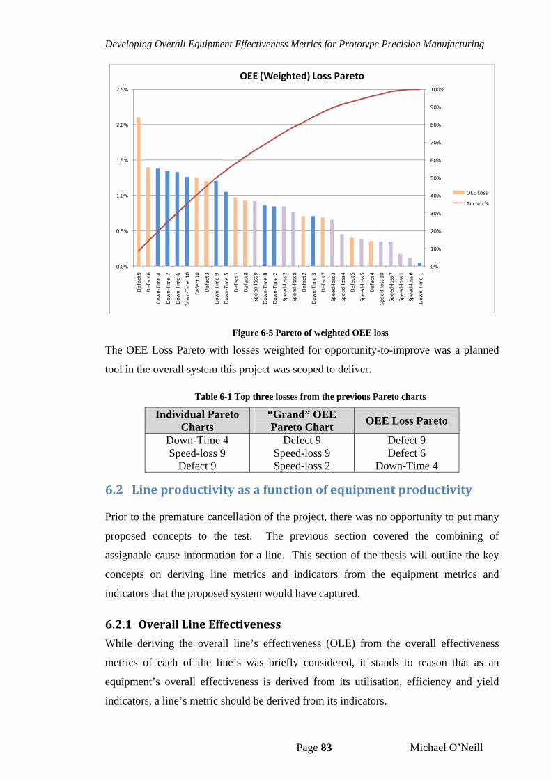
Developing Overall Equipment Effectiveness Metrics for Prototype Precision Manufacturing
Page 83 Michael O’Neill
0%
10%
20%
30%
40%
50%
60%
70%
80%
90%
100%
0.0%
0.5%
1.0%
1.5%
2.0%
2.5%
Defect 9
Defect 6
Down‐Time 4
Down‐Time 7
Down‐Time 6
Down‐Time 10
Defect 10
Defect 3
Down‐Time 9
Down‐Time 5
Defect 1
Defect 8
Speed‐loss 9
Down‐Time 8
Down‐Time 2
Speed‐loss 2
Speed‐loss 8
Defect 2
Down‐Time 3
Defect 7
Speed‐loss 3
Speed‐loss 4
Defect 5
Speed‐loss 5
Defect 4
Speed‐loss 10
Speed‐loss 7
Speed‐loss 1
Speed‐loss 6
Down‐Time 1
OEE (Weighted) Loss Pareto
OEE Loss
Accum.%
Figure 6-5 Pareto of weighted OEE loss
The OEE Loss Pareto with losses weighted for opportunity-to-improve was a planned
tool in the overall system this project was scoped to deliver.
Table 6-1 Top three losses from the previous Pareto charts
Individual Pareto Charts
“Grand” OEE Pareto Chart
OEE Loss Pareto
Down-Time 4 Speed-loss 9
Defect 9
Defect 9 Speed-loss 9 Speed-loss 2
Defect 9 Defect 6
Down-Time 4
6.2 Lineproductivityasafunctionofequipmentproductivity
Prior to the premature cancellation of the project, there was no opportunity to put many
proposed concepts to the test. The previous section covered the combining of
assignable cause information for a line. This section of the thesis will outline the key
concepts on deriving line metrics and indicators from the equipment metrics and
indicators that the proposed system would have captured.
6.2.1 OverallLineEffectiveness
While deriving the overall line’s effectiveness (OLE) from the overall effectiveness
metrics of each of the line’s was briefly considered, it stands to reason that as an
equipment’s overall effectiveness is derived from its utilisation, efficiency and yield
indicators, a line’s metric should be derived from its indicators.
Developing Overall Equipment Effectiveness Metrics for Prototype Precision Manufacturing
Page 84 Michael O’Neill
LINELINELINE YEUOLE (35)
The burden of the calculating the accumulative contribution of each equipment’s
productivity to the line’s productivity falls to how the three line indicators are
calculated.
6.2.2 Utilisation
Company-X’s current line-level utilisation metric is actually an equipment-level metric.
The bottleneck of the line is determined and Down-Time events with duration greater
than 90 seconds are captured and categorised. If this equipment the true bottleneck of
the line then there is no argument that the bottleneck equipment’s utilisation is an
accurate reflection of the line’s utilisation. This is certainly true from the standpoint
that improving the throughput on equipment upstream or downstream of the bottleneck
equipment will not improve the throughput of the line.
What is questionable is how Company-X determines the bottleneck equipment. The
bottleneck designation is assigned to Equipment-E, which is present on all lines
regardless of product or lifecycle phase. This established standard comes from
historical performance from a routing (order of equipment through which units are
processed) that is no longer in use. This legacy practice is routinely challenged by time-
studies performed by the company’s industrial engineers and become a point of
contention for the equipment-focused engineering group.
Equipment-level OEE metric captured at all the line’s equipment independently would
allow for dynamic designation of bottleneck. This allows a simple refinement of the
existing line-level utilisation indicator to use the utilisation of the equipment determined
to be the bottleneck.
Another concept that was being considered was to sum the different factors of
utilisation for all equipment on a line, Equation 9, to determine the overall utilisation
independent of the throughput bottleneck. The reasoning of this was the equipment
earlier in the PTM and PDM lines would routinely be utilised for engineering testing or
training as manufacturing build was still progressing through the remainder of the line.
This summation might better reflect the true utilisation of the line’s equipment when
different equipment on the line was used concurrently for production and non-
production activities.
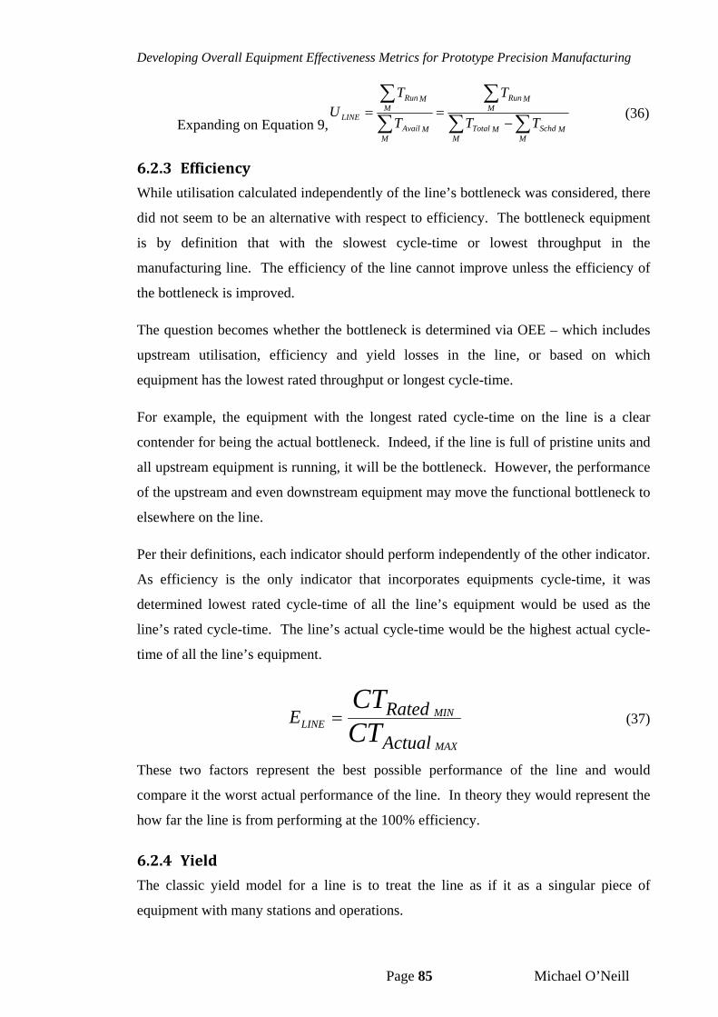
Developing Overall Equipment Effectiveness Metrics for Prototype Precision Manufacturing
Page 85 Michael O’Neill
Expanding on Equation 9,
MMSchd
MMTotal
MMRun
MMAvail
MMRun
LINE TT
T
T
TU
(36)
6.2.3 Efficiency
While utilisation calculated independently of the line’s bottleneck was considered, there
did not seem to be an alternative with respect to efficiency. The bottleneck equipment
is by definition that with the slowest cycle-time or lowest throughput in the
manufacturing line. The efficiency of the line cannot improve unless the efficiency of
the bottleneck is improved.
The question becomes whether the bottleneck is determined via OEE – which includes
upstream utilisation, efficiency and yield losses in the line, or based on which
equipment has the lowest rated throughput or longest cycle-time.
For example, the equipment with the longest rated cycle-time on the line is a clear
contender for being the actual bottleneck. Indeed, if the line is full of pristine units and
all upstream equipment is running, it will be the bottleneck. However, the performance
of the upstream and even downstream equipment may move the functional bottleneck to
elsewhere on the line.
Per their definitions, each indicator should perform independently of the other indicator.
As efficiency is the only indicator that incorporates equipments cycle-time, it was
determined lowest rated cycle-time of all the line’s equipment would be used as the
line’s rated cycle-time. The line’s actual cycle-time would be the highest actual cycle-
time of all the line’s equipment.
Actual
RatedECTCT
MAX
MINLINE
(37)
These two factors represent the best possible performance of the line and would
compare it the worst actual performance of the line. In theory they would represent the
how far the line is from performing at the 100% efficiency.
6.2.4 Yield
The classic yield model for a line is to treat the line as if it as a singular piece of
equipment with many stations and operations.
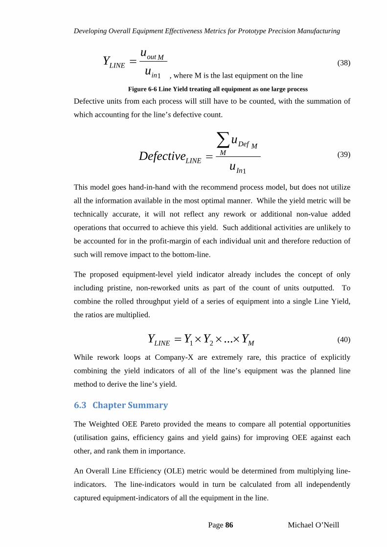
Developing Overall Equipment Effectiveness Metrics for Prototype Precision Manufacturing
Page 86 Michael O’Neill
1in
MoutLINE u
uY
, where M is the last equipment on the line
(38)
Figure 6-6 Line Yield treating all equipment as one large process
Defective units from each process will still have to be counted, with the summation of
which accounting for the line’s defective count.
1In
MMDef
LINE u
uDefective
(39)
This model goes hand-in-hand with the recommend process model, but does not utilize
all the information available in the most optimal manner. While the yield metric will be
technically accurate, it will not reflect any rework or additional non-value added
operations that occurred to achieve this yield. Such additional activities are unlikely to
be accounted for in the profit-margin of each individual unit and therefore reduction of
such will remove impact to the bottom-line.
The proposed equipment-level yield indicator already includes the concept of only
including pristine, non-reworked units as part of the count of units outputted. To
combine the rolled throughput yield of a series of equipment into a single Line Yield,
the ratios are multiplied.
MLINE YYYY ...21 (40)
While rework loops at Company-X are extremely rare, this practice of explicitly
combining the yield indicators of all of the line’s equipment was the planned line
method to derive the line’s yield.
6.3 ChapterSummary
The Weighted OEE Pareto provided the means to compare all potential opportunities
(utilisation gains, efficiency gains and yield gains) for improving OEE against each
other, and rank them in importance.
An Overall Line Efficiency (OLE) metric would be determined from multiplying line-
indicators. The line-indicators would in turn be calculated from all independently
captured equipment-indicators of all the equipment in the line.
Developing Overall Equipment Effectiveness Metrics for Prototype Precision Manufacturing
Page 87 Michael O’Neill
7 Conclusions&Recommendations
7.1 Conclusions
An OEE tracking system that added little if any extra non-value added work on
equipment operators was created. Such a system categorised its factors and sources of
loss in a manner than allowed all PTM, PDM and HVM departments focus on their
specific goals yet also allowed for correlation of performance between the phases of
program life-cycle.
An utilisation tracking system was designed to interact with an equipment’s controller
to capture and categorise all time spent on the equipment. It also ensured that the time
the equipment spent powered down is captured. The captured data required minimal
user input and was used to accurately determine the equipment’s utilisation. This
utilisation indicator provided the same functionality as the Availability Efficiency and
Operating Efficiency metrics as defined by SEMI E79.
An efficiency tracking system was designed to interact with an equipment’s computer-
controller to capture and categorise the equipment’s cycle-time. Cycle-time was
categorized as steady-state and non-steady-state such that:
Historical steady-state cycle-times from multiple instance of Equipment-Z
were used to determine Equipment-Z’s Rated Cycle-Time.
Steady-state cycle-time, or some function of non-steady-state cycle-time to
estimate steady-state, were used as Actual Cycle-Time in real time.
This efficiency indicator provided the same functionality as the Rated Efficiency metric
as defined by SEMI E79.
A yield tracking system was designed to interact with an equipment’s controller to
capture the number of units actually loaded and unloaded from the equipment as well as
the number of defective units. It also categorised, with minimal user input as needed,
the number and classification of defects detected on defective units. This yield indicator
provided the same functionality as the Quality Efficiency metric as defined by SEMI.
Developing Overall Equipment Effectiveness Metrics for Prototype Precision Manufacturing
Page 88 Michael O’Neill
OEE metrics are only valuable if the sources of OEE loss are prioritised for focused
improvement. Rather than focus on utilisation, efficiency and yield independently these
OEE losses were weighted based on opportunity and compared in the same Pareto chart.
This system was implemented on Equipment-Z on selected pilot PTM, PDM and HVM
lines at Company-X. End-users of the system and the captured data approved a final
refinement of the utilisation tracking software. Implementation was approved pending
validation of those refinements. The same tracking systems used on Equipment-Z could
be implemented on Company-X’s other equipment.
7.2 Recommendations
The following would have been developed further had opportunity allowed.
Automatic classification of efficiency loss: While the existing system at Company-X
allowed for the automatic detection of steady-state and non-steady-state, it only
provided the raw data from which engineering would have to infer opportunities for
improvement. Ideally the system would know the conditions which constituted the
equipment’s rated cycle-time, and would be able to deduce and assign causes of loss
automatically. For example, if the rated cycle-time included a “waiting for upstream
time” to be 1 second or less, and the signal from the upstream process occurred after 2
seconds, the monitoring software could recorded a speed loss of 1 second due to waiting
for upstream equipment.
Determining Overall Line Efficiency as a function of the line’s equipment’s OEE
metrics: Company-X as well as other manufacturers require the ability to correlate the
current performance of individual stand-alone equipment used for batch-volume
production during prototyping, to the future performance of fully coupled dedicated
equipment in a high-volume manufacturing line. It was proven that the same system
can work on a piece of equipment be it stand-alone or coupled, or used for batch-
volume or high-volume. Upon implementing this system on all equipment across the
line, the various proposed formulae in Section 6.2 could be evaluated.
Developing Overall Equipment Effectiveness Metrics for Prototype Precision Manufacturing
Page 89 Michael O’Neill
8 References
[1] J.K., Liker. The Toyota Way. New York : McGraw-Hill, 2004.
[2] Subramaniam, S. K., Husin, S. H., Yusop, Y. and A. H. Hamidon. Machine efficiency and man power utilization on production lines. Proceedings of the 8th WSEAS international conference on Electronics, hardware, wireless and optical communication. 2009, P. 70-75
[3] de Ron, A.J. and Rooda, J.E. Equipment effectiveness: OEE revisited. IEEE Transactions on Semiconductor Manufacturing. 2005, Vol. 18, 1.
[4] Mead, S. Improving OEE in high mix facilities. Manufacturing Engineer. 2002, Vol. 19, 9.
[5] Ljungberg, Ö. Measurement of overall equipment effectiveness as a basis for TPM activities. International Journal of Operations & Production Management. 1998, Vol. 18, 5.
[6] Sehonberger, R.J. Consider the downside of OEE. Manufacturing Engineering. 2008, Vol. 141, 6.
[7] SEMI E79 Specification for Definition and Measurement of Equipment Productivity
[8] Dal, B., Tugwell, P. and Greatbanks, R. Overall equipment effectiveness as a measure of operational improvement – A practical analysis. International Journal of Operations & Production Management. 2000, Vol. 20, 12.
[9] Killeen, D., Gaboury, P. and Paccard, D. Managing, measuring and improving equipment capacity and overall equipment efficiency (OEE) using iPLUS. Proceedings of IEEE International Symposium on Semiconductor Manufacturing . 2001, P. 25-28.
[10] Godfrey, P. Overall equipment effectiveness. Manufacturing Engineer. 2002, Vol. 81, 3.
[11] da Costa, S.E.G. and de Lima, E.P. Uses and misuses of the "'overall equipment effectiveness" for production management. IEEE International Engineering Management Conference. 2002, Vol. 2.
[12] Braglia, M., Frosolini, M. and Zammori, F. Overall equipment effectiveness of a manufacturing line (OEEML): An integrated approach to assess systems performance. Journal of Manufacturing Technology Management. 2009, Vol. 20, 1.
Developing Overall Equipment Effectiveness Metrics for Prototype Precision Manufacturing
Page 90 Michael O’Neill
[13] Clark, R. Concise OEE made E-A-S-Y. Tooling and Production. 2005, Vol. 71, 12.
[14] Garza-Reyes, J.A.,Eldridge, S., Barber, K.D. and Soriano-Meier, H. Overall equipment effectiveness (OEE) and process capability (PC) measures: a relationship analysis. International Journal of Quality & Reliability Management 2010, Vol. 27, 1.
[15] Esmaeilian, G.R., MegatAhmad, M.M.H., Ismail, N., Sulaiman, S. and Hamedi, M. Particular model for improving failure mode and effect analysis (FMEA) by using of overall equipment efficiency (OEE). Information Technology, 2008. ITSim 2008. International Symposium on. 2008, Vol. 4
[16] Batumalay, K. and Santhapparaj, A.S. Overall Equipment Effectiveness (OEE) through Total Productive Maintenance (TPM) practices - A study across the Malaysian industries. International Conference for Technical Postgraduates 2009.
[17] Steege, P. Overall equipment effectiveness in resist processing equipment. Proceedings of Advanced Semiconductor Manufacturing Conference and Workshop. 1996, P. 76-79.
[18] Kwon, O. and Lee, H. Calculation methodology for contributive managerial effect by OEE as a result of TPM activities. Journal of Quality in Maintenance Engineering. 2004, Vol. 10, 4.
[19] Foster, J., Matthews, J., Beaumont, P., Zarbock, T. and Yeo, D.. Equipment Throughput Optimization by Means of Speed Loss Analysis. IEEE Transactions on Semiconductor Manufacturing. 2008, Vol. 21, 3.
[20] Gililland, J., Konopka, J., Barber K., Schnabl R. and Ames, V. A. Semiconductor Manufacturing Productivity Overall Equipment Effectiveness (OEE) Guidebook. SEMATECH. 1995, Revision 1.
[21] O’Neill, M. Development of Knowledge-Based System for Quality Control Improvement. Dublin City University School of Mechanical and Manufacturing Student Undergraduate Thesis. 2002
[22] Ray, D. Beyond OEE: 5 steps to success. Plant Engineering. 2008, Vol. 62, 3.
[23] Freck, Robert W. Using overall equipment effectiveness (OEE) and the equipment improvement process (EI) to improve fab throughput. Proceedings of IEEE International Symposium on Semiconductor Manufacturing Conference. 2000, P. 469-471.
[24] Brochu, D.L. OEE: using metrics to manage, improve performance. Plant Engineering. 2007, Vol. 61, 6.
Developing Overall Equipment Effectiveness Metrics for Prototype Precision Manufacturing
Page 91 Michael O’Neill
[25] Angeles, E., Rajput, K., Cruz, M., Almonte, A., Libiran, I., Minor, K., Realdy, A., Li, M., Karr, R., Buchanan, M. and Ajouri, S. Burn-in operations improvement with full automation and OEE/OEU. International Symposium on Semiconductor Manufacturing. 2007, P. 525-528.
[26] Gleason, M. High level of operating equipment efficiency requires overall effort. Pulp and Paper. 1995, Vol. 69, 7.
[27] Berndlmaier, Z., et al. The Grand Pareto: A Methodology for Identifying and Quantifying Yield Detractors in a Technology for Volume Semiconductor Manufacturing. Advanced Semiconductor Manufacturing Conference. 2006.
[28] Oechsner, R., Pfeffer, M., Pfitzner, L., Binder, H., Muller, E., Vonderstrass, T. From overall equipment efficiency (OEE) to overall Fab effectiveness (OFE). Materials Science in Semiconductor Processing. 2002, Vol. 5, 4-5.
[29] Muchiri, P. and Pintelon, L. Perormance measurement using overall equipment effectiveness (OEE): literature review and practical application discussion. International Journal of Production Research. 2008, Vol. 46, 13.
[30] [Author Unknown] OEE for smaller batch machining. Metalworking Production. 2004, Vol. 148, 13.
[31] Nachiappan, R.M. and Anantharaman N. Evaluation of overall line effectiveness (OLE) in a continuous product line manufacturing system). Journal of Quality in Maintenance Engineering. 2006, Vol. 17, 7.
[32] Jonsson, P. and Lesshammar, M. Measuring manufacturing performance: dimensions and OEE. ortland International Conference on Management of Engineering Technology. 1997, P. 799.
[33] Giegling, S., Haymon, T., Verdini, W.A. and Konopka, J. Implementation of overall equipment effectiveness (OEE) system at a semiconductor manufacturer. Proceedings of the IEEE/CPMT International Electronics Manufacturing Technology (IEMT) Symposium. 1997, P. 93-98.
[34] Jusko, J. OEE: the heart of the matter. Industry Week. 2009, Vol. 258, 2.
[35] Raleigh, P . OEE goes paper-free . Process Engineering . 2008, Vol. 89, 5.
[36] Bamber, C.J., et al. Cross-functional team working for overall equipment effectiveness (OEE). Journal of Quality in Maintenance Engineering. 2003, Vol. 9, 3.

Developing Overall Equipment Effectiveness Metrics for Prototype Precision Manufacturing
Page 92 Michael O’Neill
[37] Nakajima, S. An Introduction to TPM. Productivity Press, Cmbridge, MA. 1988.
[38] London, A. and Segev, D. Implementing a world-class OEE management system. Solid State Technology. 2003, Vol. 46, 6.
[39] Loughlin, S. A holistic approach to overall equipment effectiveness (OEE). IEE Computing and Control Engineering. 2003, Vol. 14, 6.
[40] Pomorski, T. Managing overall equipment effectiveness [OEE] to optimize factory performance. Semiconductor Manufacturing Conference Proceedings, 1997 IEEE International Symposium on. 1997.
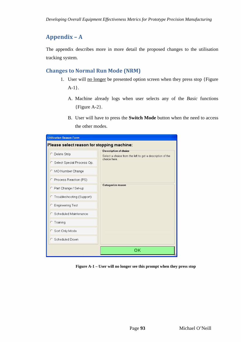
Developing Overall Equipment Effectiveness Metrics for Prototype Precision Manufacturing
Page 93 Michael O’Neill
Appendix–A
The appendix describes more in more detail the proposed changes to the utilisation
tracking system.
ChangestoNormalRunMode(NRM)1. User will no longer be presented option screen when they press stop {Figure
A-1}.
A. Machine already logs when user selects any of the Basic functions
{Figure A-2}.
B. User will have to press the Switch Mode button when the need to access
the other modes.
Figure A-1 – User will no longer see this prompt when they press stop
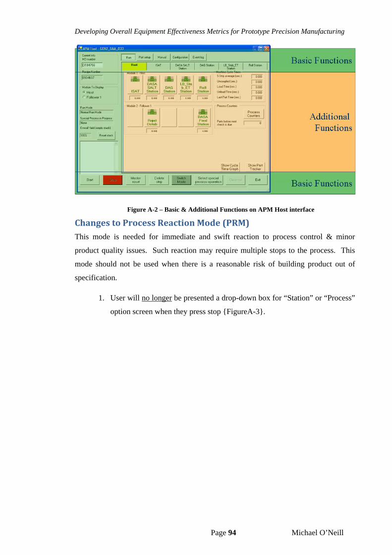
Developing Overall Equipment Effectiveness Metrics for Prototype Precision Manufacturing
Page 94 Michael O’Neill
Figure A-2 – Basic & Additional Functions on APM Host interface
ChangestoProcessReactionMode(PRM)This mode is needed for immediate and swift reaction to process control & minor
product quality issues. Such reaction may require multiple stops to the process. This
mode should not be used when there is a reasonable risk of building product out of
specification.
1. User will no longer be presented a drop-down box for “Station” or “Process”
option screen when they press stop {FigureA-3}.
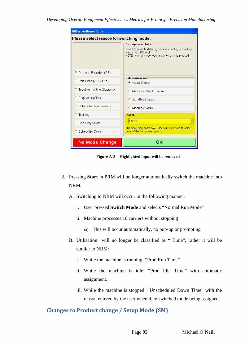
Developing Overall Equipment Effectiveness Metrics for Prototype Precision Manufacturing
Page 95 Michael O’Neill
Figure A-3 – Highlighted input will be removed
2. Pressing Start in PRM will no longer automatically switch the machine into
NRM.
A. Switching to NRM will occur in the following manner:
i. User pressed Switch Mode and selects “Normal Run Mode”
ii. Machine processes 10 carriers without stopping
(a) This will occur automatically, no pop-up or prompting
B. Utilisation will no longer be classified as “ Time”, rather it will be
similar to NRM:
i. While the machine is running: “Prod Run Time”
ii. While the machine is idle: “Prod Idle Time” with automatic
assignment.
iii. While the machine is stopped: “Unscheduled Down Time” with the
reason entered by the user when they switched mode being assigned.
ChangestoProductchange/SetupMode(SM)
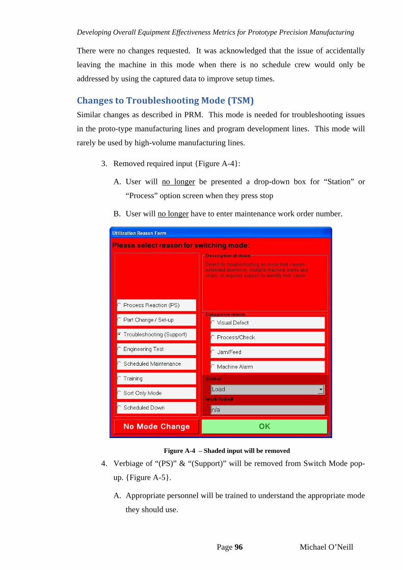
Developing Overall Equipment Effectiveness Metrics for Prototype Precision Manufacturing
Page 96 Michael O’Neill
There were no changes requested. It was acknowledged that the issue of accidentally
leaving the machine in this mode when there is no schedule crew would only be
addressed by using the captured data to improve setup times.
ChangestoTroubleshootingMode(TSM)Similar changes as described in PRM. This mode is needed for troubleshooting issues
in the proto-type manufacturing lines and program development lines. This mode will
rarely be used by high-volume manufacturing lines.
3. Removed required input {Figure A-4}:
A. User will no longer be presented a drop-down box for “Station” or
“Process” option screen when they press stop
B. User will no longer have to enter maintenance work order number.
Figure A-4 – Shaded input will be removed
4. Verbiage of “(PS)” & “(Support)” will be removed from Switch Mode pop-
up. {Figure A-5}.
A. Appropriate personnel will be trained to understand the appropriate mode
they should use.
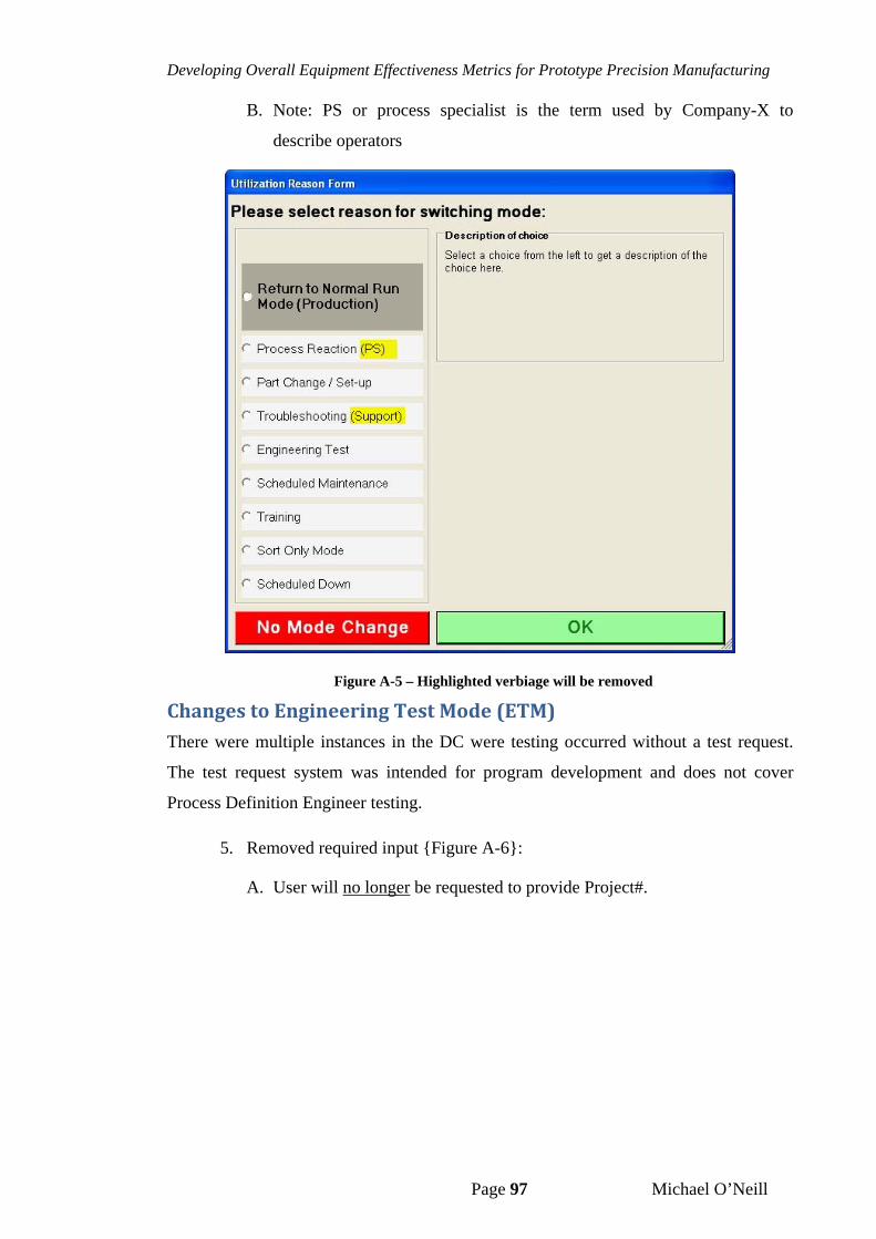
Developing Overall Equipment Effectiveness Metrics for Prototype Precision Manufacturing
Page 97 Michael O’Neill
B. Note: PS or process specialist is the term used by Company-X to
describe operators
Figure A-5 – Highlighted verbiage will be removed
ChangestoEngineeringTestMode(ETM)There were multiple instances in the DC were testing occurred without a test request.
The test request system was intended for program development and does not cover
Process Definition Engineer testing.
5. Removed required input {Figure A-6}:
A. User will no longer be requested to provide Project#.
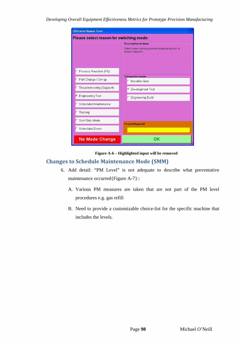
Developing Overall Equipment Effectiveness Metrics for Prototype Precision Manufacturing
Page 98 Michael O’Neill
Figure A-6 – Highlighted input will be removed
ChangestoScheduleMaintenanceMode(SMM)6. Add detail: “PM Level” is not adequate to describe what preventative
maintenance occurred{Figure A-7}::
A. Various PM measures are taken that are not part of the PM level
procedures e.g. gas refill
B. Need to provide a customizable choice-list for the specific machine that
includes the levels.
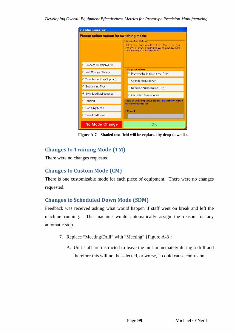
Developing Overall Equipment Effectiveness Metrics for Prototype Precision Manufacturing
Page 99 Michael O’Neill
Figure A-7 – Shaded text field will be replaced by drop-down list
ChangestoTrainingMode(TM)There were no changes requested.
ChangestoCustomMode(CM)There is one customizable mode for each piece of equipment. There were no changes
requested.
ChangestoScheduledDownMode(SDM)Feedback was received asking what would happen if staff went on break and left the
machine running. The machine would automatically assign the reason for any
automatic stop.
7. Replace “Meeting/Drill” with “Meeting” {Figure A-8}:
A. Unit staff are instructed to leave the unit immediately during a drill and
therefore this will not be selected, or worse, it could cause confusion.
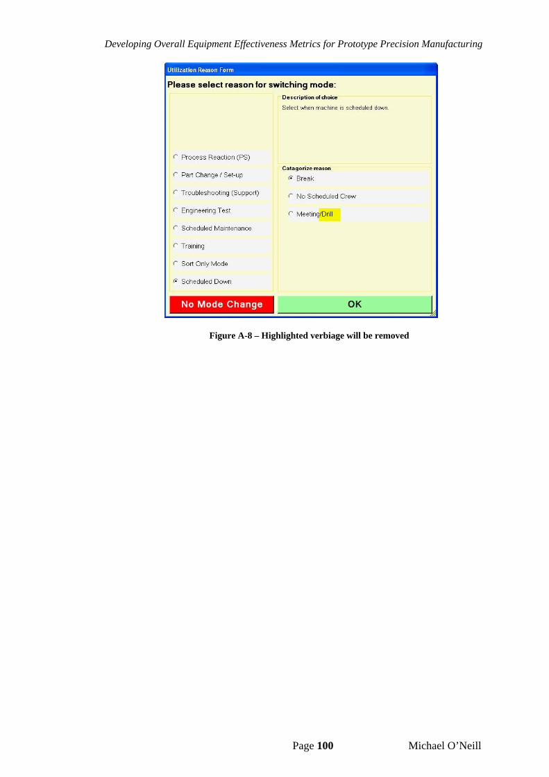
Developing Overall Equipment Effectiveness Metrics for Prototype Precision Manufacturing
Page 100 Michael O’Neill
Figure A-8 – Highlighted verbiage will be removed
Developing Overall Equipment Effectiveness Metrics for Prototype Precision Manufacturing
Page 101 Michael O’Neill
Appendix – B: Changes within Company‐X and impact to
project
Despite the backing of management from the manufacturing and engineering
departments at each of the company’s plants, progress on the design and development
of the OEE tracking system was fraught with setbacks. These are likely typical for
many manufacturing environments with multiple overlapping departments and different
management in different locations.
None of these setbacks were as significant as the company’s need to restructure in
December 2008, the full affects of which were not completely understood until June
2009. One of the HVM-focused plants was closed, with the PTM/PDM-focused plant
gaining HVM duties. Approximately 25% of the work-force were either laid-off or
voluntarily departed the company. This all resulted in:
The dissolution of the department that commissioned the project
The loss of all major project sponsors, via reassignment or departure
A significant change of internal goals and focus on surviving the global
economic recession
The long-term effort for a company-wide implementation of the system was shelved.
The completed development and implementation of the designed system on a single set
of equipment did not make business sense.
OEE improvement was no longer a priority at Company-X as demand had dropped to
level where there was excess capacity. The software and documented development
activities, results and decision were retained. Assuming the company’s survival and
growth OEE improvement would be needed in the future. At such time a system that
was already proved to capture utilisation, efficiency and yield could be implemented on
Equipment-Z. In turn Equipment-Z would serve as the model needed to implement all
throughout the line.