Embed Size (px)
Citation preview
Equilibrium Welfare and Government Policywith Quasi-Geometric Discounting
Per Krusell, Burhanettin Kuruscu, and Anthony A. Smith, Jr.∗
August 2001
∗Per Krusell and Burhanettin Kuruscu are at the Department of Economics, Harkness Hall, Univer-sity of Rochester, Rochester, NY 14627, telephone (716) 273-4903, fax (716) 271-3900, and [email protected] and [email protected], respectively; Krusell is alsoat the Institute for International Economic Studies and the CEPR; Anthony A. Smith, Jr. is atGraduate School of Industrial Administration, Carnegie Mellon University, Pittsburgh, PA 15213,telephone (412) 268-7583, fax (412) 268-7357, e-mail [email protected]. Krusell and Smiththank the National Science Foundation for financial support.
1
ABSTRACT
We consider a representative-agent equilibrium model where the consumer has quasi-geometricdiscounting and cannot commit to future actions. We restrict attention to a parametric classfor preferences and technology and solve for time-consistent competitive equilibria globally andexplicitly. We then characterize the welfare properties of competitive equilibria and compare themto that of a planning problem. The planner is a consumer representative who, without commitmentbut in a time-consistent way, maximizes his present-value utility subject to resource constraints.The competitive equilibrium results in strictly higher welfare than does the planning problemwhenever the discounting is not geometric. Journal of Economic Literature Classification Numbers:E21, E61, E91.
Keywords: quasi-geometric discounting, Markov equilibrium, taxation, time-consistent policy.
2
1 Introduction
Experimental psychology has gathered a significant body of evidence that “preference reversals”
are a common occurrence in decision making over time (see, e.g., Ainslie [1]). One expression of
these findings is that discounting of future rewards is not geometric—the standard case considered
in economics—but rather hyperbolic, or “quasi-hyperbolic”.1 A view of these findings commonly
expressed by economists is that experiments in general are fraught with problems and should be
disregarded, or, as a less extreme position, that these particular experiments suffer from specific
problems, thus including the possibility that there are alternative interpretations of the experimen-
tal results that are not in contradiction with our standard assumptions about preferences. However,
a dismissal of the psychologists’ findings seems hazardous, since they quite strongly suggest a “fric-
tion” that may be an important part of economic welfare and, possibly, also one where government
intervention might be helpful. In this paper we take the latter view: we admit the possibility that
consumption-savings decisions are indeed made by agents whose preferences allow reversals. In par-
ticular, we assume quasi-geometric preferences, which is the very simplest kind of departure from
our standard assumption on discounting.2 We assume that the time-inconsistency in preferences
is accompanied by an inability of consumers to commit to future actions, but view consumers as
fully rational: they are aware of their “internal friction” and do their best to minimize its effects.
Our main goal here is the most basic question to an economist: we perform welfare analysis of the
market mechanism. The question is: does the “invisible hand” work as well as in the standard
case, or would government intervention be desirable?
We show, first, that the standard recursive tools used to analyze the neoclassical-growth,
general-equilibrium framework can be employed also in the case of quasi-geometric preferences.
A consumer in our economy plays a game with his future selves, with whom he disagrees about
how to save, and a key part of his decisions is about how to manipulate his future savings decisions
by saving differently today. This is also a way of thinking about the geometric case, with the differ-
ence that there, no disagreements occur, and manipulation is superfluous. We restrict attention to
Markov (time-consistent) equilibria which are limits of finite-horizon equilibria, thereby obtaining
uniqueness in our specific functional-form examples and allowing straightforward welfare analysis
and comparative-static exercises.
For the welfare analysis, we assume that the “visible hand” in our economy—a planner with the
ability to command consumption decisions, or a government with the possibility of using taxes to
distort these decisions—is subject to the same friction as are consumers: it cannot commit its future
behavior. So to the extent that it shares the consumers’ preferences, it also will have preference
reversals, and will want to manipulate its future actions. It is well known that if the government
can commit, then it can help consumers achieve higher ex-ante welfare, but it is not at all clear
3
to us how the government could provide a general commitment technology for consumers’ future
consumption decisions. If it could commit to paths of future tax rates, it would be helpful, but if it
is benevolent and shares the (combination of the current and future) consumers’ preferences, such
choices are not time-consistent and are thus not likely to be realized. Although we do think that
some government commitment may be feasible, we do not think a full ability to commit is likely.
Whatever lack of commitment remains is the subject of this paper.
Our results are rather striking. We find that, whenever there is a time-inconsistency in pref-
erences, not only does a benevolent-social-planning economy not deliver the same consumption
allocation as does a laissez-faire world, but it delivers strictly lower welfare. Thus, we find a new
argument for why the market mechanism is a particularly good one. The key insight regards price-
taking behavior, as opposed to taking into account the impact of one’s decisions on prices (or
aggregate allocations). An alternative interpretation of the result is that a decentralization with
many identical Robinson Crusoes each operating their own production technology would do as
poorly as the visible-hand world: a separation of consumption and production decisions is desirable
in this economy.
The mechanism behind our main finding is intuitive and can be understood as follows. Suppose
that the social planner’s preferences coincide exactly with those of the current consumer. They
would then both regard their respective future selves as saving too little (the argument focuses on
this particular bias for illustration). As a consequence, they would both want to manipulate their
future selves. The manipulation occurs via savings (which is their only decision variable here):
when an extra dollar is saved, the extra income next period will influence savings next period.
With time-consistent preferences, the current saver agrees with his future self about next period’s
savings decision, and an envelope argument allows him to ignore this effect when deciding on current
savings. Here, in contrast, an extra dollar saved today has an additional benefit next period, since
(so long as the marginal savings propensity is not negative or zero) it induces more future savings.
The difference between the decentralized allocation and the central planning allocation originates
in how these induced future increases in savings are perceived: they are perceived as being larger
by a price-taker than by a planner. The reason for this is that the price-taker’s future behavioral
response is “more linear”: the added income he obtains next period is the higher savings times
the return, which he perceives as constant. The planner, on the other hand, sees that for every
additional dollar saved, the next period’s return falls (assuming decreasing marginal productivity
to capital). In sum, the incentives to save are higher for the decentralized agents, so they save more,
and more saving is better in this economy: it takes us closer to the full commitment outcome.3
The most closely related literature to this paper is the set of studies started by Strotz [21]
and Phelps and Pollak [18] and then further developed recently in a set of papers Laibson, e.g.,
Laibson [13]. Laibson [14] discusses some aspects of government taxation, but does not consider
4

the case when the government cannot commit its future tax rates, the main focus of our analysis
here. In many of Laibson’s setups (e.g., Laibson [15]), there are added market frictions, such as
credit constraints, which makes illiquid assets play an important role. As a consequence, Ricardian
equivalence does not hold. Another common assumption is the existence of partially uninsurable
idiosyncratic shocks (Harris and Laibson [6]). Here, the setup is the most basic one possible: the
only friction is the internal friction in consumers’ preferences (naturally accompanied with a lack
of commitment), and there is no uncertainty. In particular, all long- and short-term asset markets
are operative; although it would be beneficial to close asset markets in the future, without the
commitment power to do so, ex post it will always be in the interest of the group of consumers
as a whole to keep current markets open. As a result, in our environment, Ricardian equivalence
holds. Another example of an added friction is the one considered in O’Donoghue and Rabin [17],
where in one version of their model consumers are not rational, but are rather constantly surprised
at their preference reversals.
The analysis in the paper builds fundamentally on recursive methods, and moreover uses specific
functional forms so as to allow manageable closed-form solutions. The dynamic game thus played
between the current and future selves is perhaps the simplest tractable example of a time-consistent
equilibrium available in the literature. This literature began in Kydland and Prescott [12] but
has not allowed simple closed-form examples of Markov equilibria. We consider the case with a
saver with time-inconsistent preferences as very natural grounds for illustrating the main forces
at work. Central to this illustration are the recursive setup and the derivation and discussion
of the “generalized Euler equation”. Section 2 describes the basic setup and the principles we
follow in our analysis. Section 3 introduces recursive competitive equilibrium (without policy),
and Section 4 considers the planning problem, including the comparison with the competitive
equilibrium outcome. Section 5 looks at time-consistent policy: we show that the planning outcome
is also the outcome of a government policy game, provided the government has a sufficiently large
set of instruments. Section 6 concludes, discusses some weaknesses in the analysis, and mentions
an alternative approach.
5
2 The Setup
2.1 Primitives
Time is discrete and infinite and begins at time 0; there is no uncertainty. An infinitely-lived
consumer derives utility from a stream of consumption at different dates. We assume that the
preferences of this individual are time-additive, and that they take the form of a sequence of
preference profiles:
U0 = u0 + β(δu1 + δ2u2 + δ3u3 + . . .
)U1 = u1 + β
(δu2 + δ2u3 + . . .
)U2 = u2 + β (δu3 + . . .)
When β = 1, we have standard, time-consistent, geometric preferences. When β 6= 1, there is a
time-inconsistency: at date 0, the trade-off between dates 1 and 2 is perceived differently than at
date 1, and so on. When β < 1, we have “excessive short-run impatience”: the individual thinks
“I want to save, just not right now”; when β > 1, excessive short-run patience is expressed as “I
want to consume, just not right now”. We refer to this class of preferences as quasi-geometric, as
they are a one-period deviation from the standard geometric case.4 Successively more complicated
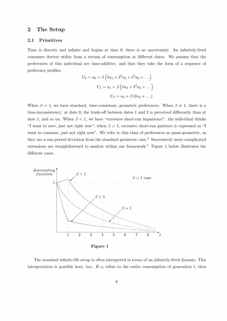
extensions are straightforward to analyze within our framework.5 Figure 1 below illustrates the
different cases.
-
6
��
��
��
��
��
�
discountingfunction
1δ < 1 case
β > 1
β < 1
β = 1
1 2 3 4 5 6 7 8 t
Figure 1
The standard infinite-life setup is often interpreted in terms of an infinitely-lived dynasty. This
interpretation is possible here, too. If ct refers to the entire consumption of generation t, then
6
the assumption of quasi-geometric discounting implies a version of “impure” altruism: although
the generation t agent cares about the consumption of all his descendants, he disagrees with his
descendants on the weights. For example, he places a higher weight on the consumption of his
grandchildren relative to his children than do his children. Thus, with dynasties in mind, the
dynamic game we study here can be thought of as a game between different generations.
2.2 Modelling behavior under time-inconsistent preferences
As time progresses, the individual will change his mind about the relative values of consumption
at different points in time so long as β 6= 1. He would, therefore, if he could, commit his future
consumption levels. We assume that there is no way for the consumer to do so. This is a rather
natural assumption in a framework with time-inconsistent preferences. The reason is that com-
mitment contracts would have to be quite elaborate to avoid renegotiation problems. Suppose two
consumers, A and B, agree on a contract whereby consumer B would punish consumer A for any
deviation from the planned future consumption. For his services, consumer B would be paid some
reward. At the future date, however, consumer A would be able to convince consumer B not to
carry out the punishment: A would just offer slightly more than the original reward to B for tear-
ing the contract instead of adhering to it. Hence, unless the two consumers were playing a infinite
game, renegotiation would always make both consumers better off ex post, and any forward-looking
consumer would not bother to set up a commitment contract. The fact that a truly infinite horizon
is necessary for commitment contracts to work is an argument that makes anonymous markets
unlikely suppliers of commitment services in practice, and we believe that it is an important reason
why we do not observe such a market.6 In our model, the horizon is infinite, but we make a general
restriction to Markov strategies in our work—one that we discuss below—and one consequence of
this restriction is that commitment cannot be achieved.
Further, we assume that the consumer realizes that his preferences will change and makes
the current decision taking this into account—this encapsulates our notion of rationality in this
framework.7 This means that we model the decision-making process as a dynamic game, with the
agent’s current and future selves as players.
For our game, we focus on (first-order) Markov equilibria: at a moment in time, no histories
are assumed to matter for outcomes beyond what is summarized in the current stock of wealth
held by the agent. This means that we rule out trigger-strategy equilibria of the kind studied in
Laibson [13] and Bernheim, Ray, and Yeltekin [3].8 Further, we restrict attention to those Markov
equilibria which are limits of finite-horizon equilibria. This refinement eliminates a large number of
equilibria: Krusell and Smith [11] show that there is a large set of equilibria for this game even when
attention is restricted to first-order Markov equilibria. How many equilibria remain is in general
7
not known, but for the specific parametric case that allows a closed-form solution, there is only
one remaining equilibrium. This can be shown by explicit backward solution of the finite-horizon
model. The resulting equilibrium thus generalizes the standard preference setup in a continuous
manner. Our ability to establish uniqueness relies on restrictive assumptions on technology and
preferences—we use closed-form solutions. However, for a slightly larger parametric class that does
not allow closed-form solutions, we solve for equilibria numerically and do not find any evidence
that the limits of finite-horizon equilibria are not unique.
2.3 Assumptions on primitives
In order to obtain closed-form solutions, we restrict preferences and technology to specific functional
forms. The period utility function is u(c) = log c. We assume that 0 < δ < 1 and that β > 0.
Production is Cobb-Douglas and there is full depreciation so the resource constraint reads
c+ k′ = Akα.
Primes denote consecutive-period values.
Perfect competition implies marginal-product pricing of the capital and labor inputs:
r = αAkα−1
w = (1− α)Akα.
2.4 Recursive formulation of the decision making
Assume that the current self perceives future savings decisions to be given by a function g(k):
kt+1 = g(kt).
Note that, by the Markov assumption, g is time-independent and only has current capital as an
argument.
The current self solves
V0(k) ≡ maxk′
u(rk + w − k′) + βδV (k′),
where
V (k) = u(rk + w − g(k)) + δV (g(k)).
Notice that successive substitution of V into the objective generates the right objective if the
expectations of future behavior are given by the function g.
A solution to the current self’s problem is denoted g(k). We have a solution to the agent’s game
(i.e., to the game between the different selves) if the fixed-point condition g(k) = g(k) is satisfied
for all k.
8
Parenthetically, the commitment solution would be obtained if the expression for V instead
satisfied the standard dynamic programming functional equation
V (k) = maxk′
u(rk + w − k′) + δV (k′),
which would yield a g function that differs from g so long as β 6= 1; g would be used at time 0, and
the g forever after.
2.5 Constant prices: an explicit solution
If the prices r and w in the previous section are constant and exogenous, then, with our parametric
assumptions, we can solve explicitly for the equilibrium decision rule and corresponding value
function. In particular, the value function takes the form V (k) = a+ b log(k+ wr−1), where k+ w
r−1
is proportional to the present value of the agent’s lifetime wealth W ≡ rk + w∑∞i=0
1ri . The
equilibrium decision rule takes the form g(k) = s(rk + r
r−1w)− w
r−1 , where s = βδ1−δ(1−β) . It is not
too hard to see that this decision rule implies that W ′ = srW , that is, the agent saves a constant
fraction of his wealth in each period.
On a stationary point, where the individual’s capital stock does not change, we have g (k) = k
and W ′ = W . This implies r = 1s , a requirement for a steady state in the general equilibrium
model, which in turn equals 1−δ(1−β)βδ . This means that w
r−1 = s rr−1w. The left-hand side of this
equality is present value of future labor income; the right-hand side is equal to the savings out of
the present value of total labor income. These two need to be equal to each other in equilibrium.
As we will show, this kind of condition will also hold off the steady state in the economy with our
particular functional-form assumptions.
3 Recursive Competitive Equilibrium
Before we move on to the formal definition of a recursive competitive equilibrium, we need to
describe the market structure. Our assumption here is that the consumer rents his capital and labor
services to firms, treating prices parametrically. Further, the consumer makes the accumulation
decisions for capital. If we assumed that firms made these decisions and that consumers had access
to markets for one-period loans, the results would not change. The addition of multiperiod assets
would also not change our results: these assets would be priced using arbitrage and their returns
would be given by the returns on the relevant one-period assets. If one-period assets did not exist,
the results would change. However, with a similar argument as the one used above, it would always
be in the interest of consumers ex post to open one-period asset markets, and the spirit we follow
here is to treat consumers as fully rational at any moment in time. Thus, the natural benchmark
for us is to assume that one-period asset markets are open.
9
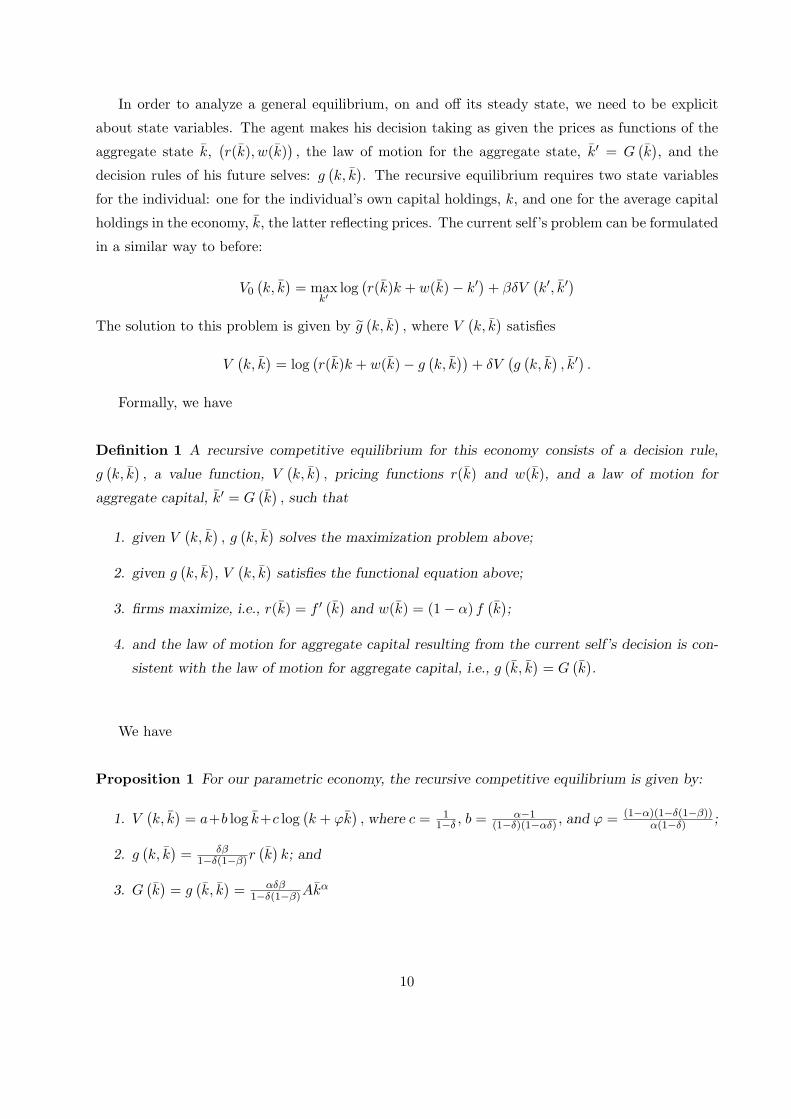
In order to analyze a general equilibrium, on and off its steady state, we need to be explicit
about state variables. The agent makes his decision taking as given the prices as functions of the
aggregate state k,(r(k), w(k)
), the law of motion for the aggregate state, k′ = G
(k), and the
decision rules of his future selves: g(k, k
). The recursive equilibrium requires two state variables
for the individual: one for the individual’s own capital holdings, k, and one for the average capital
holdings in the economy, k, the latter reflecting prices. The current self’s problem can be formulated
in a similar way to before:
V0(k, k
)= max
k′log
(r(k)k + w(k)− k′
)+ βδV
(k′, k′
)The solution to this problem is given by g
(k, k
), where V
(k, k
)satisfies
V(k, k
)= log
(r(k)k + w(k)− g
(k, k
))+ δV
(g(k, k
), k′).
Formally, we have
Definition 1 A recursive competitive equilibrium for this economy consists of a decision rule,
g(k, k
), a value function, V
(k, k
), pricing functions r(k) and w(k), and a law of motion for
aggregate capital, k′ = G(k), such that
1. given V(k, k
), g(k, k
)solves the maximization problem above;
2. given g(k, k
), V
(k, k
)satisfies the functional equation above;
3. firms maximize, i.e., r(k) = f ′(k)
and w(k) = (1− α) f(k);
4. and the law of motion for aggregate capital resulting from the current self’s decision is con-
sistent with the law of motion for aggregate capital, i.e., g(k, k
)= G
(k).
We have
Proposition 1 For our parametric economy, the recursive competitive equilibrium is given by:
1. V(k, k
)= a+b log k+c log
(k + ϕk
), where c = 1
1−δ , b = α−1(1−δ)(1−αδ) , and ϕ = (1−α)(1−δ(1−β))
α(1−δ) ;
2. g(k, k
)= δβ
1−δ(1−β)r(k)k; and
3. G(k)
= g(k, k
)= αδβ
1−δ(1−β)Akα
10
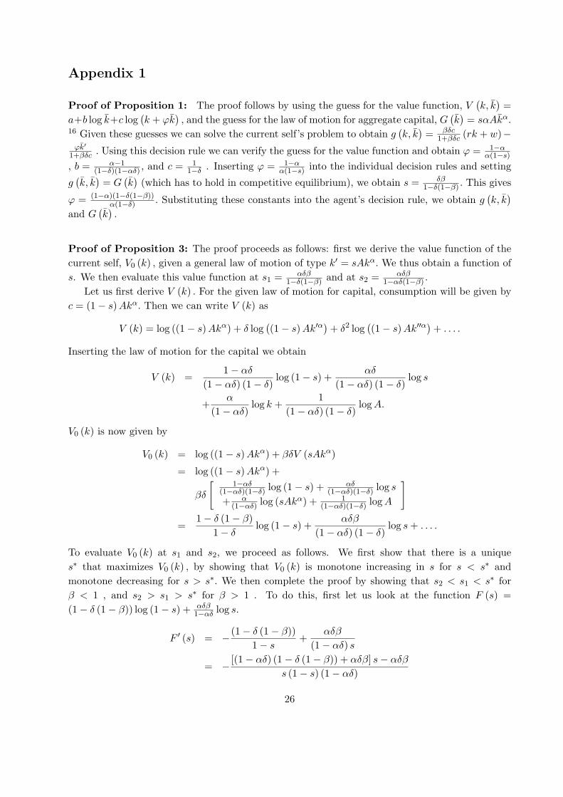
Proof: See Appendix 1.
The proof uses the intuition developed in the partial equilibrium case. Notice that the equilib-
rium savings rates in the partial equilibrium and the general equilibrium solutions are the same.
We have also suppressed the discussion of other equilibria; all equilibria calculated in this paper
are limits of finite-horizon equilibria, and as such are unique.
We now turn to the equivalence of the aggregate statistics across models with time-consistent
and time-inconsistent preferences (this is a result parallel with that found in Barro [2] for a
continuous-time model).
Proposition 2 The laws of motion for capital are the same for any two models(β, δ
)and (β, δ)
such that δβ
1−δ(1−β) = δβ1−δ(1−β) .
The proposition implies that it is not possible to estimate (β, δ) by looking at aggregates (or
disaggregated variables, for that matter) for the class of preferences and technology that we con-
centrate on. As a special case, note that the outcome of the model with (β, δ) , is identical to the
outcome of the standard growth model with δ = δβ1−δ(1−β) .
The observational equivalence simplifies presentation here, but does not eliminate the issue we
are interested in: the welfare properties of equilibria, and policy analysis. As we will see, welfare
properties across models with different underlying preferences but the same equilibrium laws of
motion can be very different.
4 Welfare Properties
Welfare properties are usually discussed in terms of the Pareto criterion. Since we are considering
an economy with lack of commitment as a central element, it is difficult to formalize this criterion:
moving allocations freely around over time violates the assumption of a lack of commitment. We
will phrase our discussion in terms of a central planning problem; we will define such a problem,
and then compare its solution to the competitive equilibrium. In contrast to a Pareto problem, the
central planning problem we formulate does not necessarily have a solution with “good” welfare
properties.
There is no obvious best notion of a planner here, since the consumer’s different selves disagree.
However, although one could think of a “meta-planner” placing positive weights on the lifetime
utilities of more than the current self, we do assume here that the planner simply shares the
preferences of the current self.9 That is, by a central planning solution we simply mean a solution
11

which would be chosen by a benevolent representative of the consumers who had the ability to
manipulate the current economic choice variables costlessly. Thus, we want to think of the analysis
of the benefits of markets as a simple “invisible hand” versus “visible hand” comparison, in the
spirit of Adam Smith.
An important reason for adopting this specific planner is found in Section 5 below. There we
show that if one formalizes the notion of a government with a sufficiently large set of tax instruments
representing the preferences of its current electorate, the resulting allocation coincides with the one
we obtain in our fictitious planning economy. Finally, and as motivated above, we further assume
that the planner cannot directly affect his future choices, thereby having to play a game with his
future selves, just like the consumer does in a competitive equilibrium.
4.1 The planning problem
In summary, in this section we assume the following: (i) the planner is a consumer representative:
he inherits his (time-inconsistent) preferences; (ii) he faces the same problem as the consumer: he
cannot commit to future actions; (iii) we require a time-consistent solution to the planner’s problem
(future planners’ reactions are taken into account in a rational way).
The differences between the consumer’s equilibrium problem and the planner’s problem are thus
as follows: (i) the consumer takes prices as given, whereas the planner has a resource constraint; and
(ii) the equilibrium consumer deals with different future players (the consumer’s future price-taking
selves) than the planner does (the planner’s future selves).
The problem of the planner’s current self can be formulated in the following way:
V0(k) ≡ maxk′
u(f(k)− k′) + βδV (k′),
where
V (k) = u(f(k)− h(k)) + δV (h(k)).
A solution to the problem of the planner’s current self is denoted h(k). We have a solution
to the planner’s game (i.e., to the game between the planner’s different selves) if the fixed-point
condition h(k) = h(k) is satisfied for all k.
It is straightforward to show that the following functions are solutions to the planner’s game:
k′ = h(k) =βδ
1− αδ(1− β)αAkα
and
V (k) = a+ b log k,
where a and b have simple closed-form solutions in terms of our parameters.
12
4.2 The planning outcome vs. the competitive outcome
Apparently, whenever α < 1, the competitive equilibrium and the planning problem produce differ-
ent outcomes. When β < 1, the price-taking agent saves more than the planner does; when β > 1,
the planner saves more. Neither the planner’s solution nor the competitive equilibrium outcome
coincide with the full commitment solution. The commitment solution for this economy has one
savings rate at time 0 and another, higher, one at all future times. The time-0 commitment rate
is equal to the savings rate of the planning problem without commitment; the subsequent savings
rate is higher (lower) than both the competitive and the no-commitment planning outcomes when
β < (>) 1.
Turning to a welfare comparison between the competitive equilibrium and the planning solution,
we have the following.
Proposition 3 The competitive outcome results in strictly higher welfare for the consumer than
the planning outcome does, whenever β 6= 1 and α < 1.
Proof: See Appendix 1.
Thus, markets outperform a benevolent social planner in this economy; in particular, competi-
tive behavior results in higher savings (when β < 1), and since there is undersaving relative to the
full commitment case, higher savings moves the economy in the right direction. What explains this
finding? As pointed out above, it should not be surprising that the two allocations are different.
The planning problem is not a standard planning problem; in particular, the planner faces a differ-
ent environment than do the competitive consumers: they face different future players, whom they
cannot fully control. In order to explain why the planner faces future players that induce worse
outcomes, we will make use of the generalized Euler equation in each case.
4.3 The generalized Euler equation
A simple derivation of the generalized Euler equation (GEE), which can be used whenever the value
function and the policy function are differentiable, goes as follows. Consider the problem of the
planner. His first-order condition reads
u′(f(k)− h(k)) = βδV ′(h(k)).
To eliminate the unknown function V ′, take derivatives of the functional equation for V :
V ′(k) = u′(f(k)− h(k))(f ′(k)− h′(k)) + δV ′(h(k))h′(k).
13
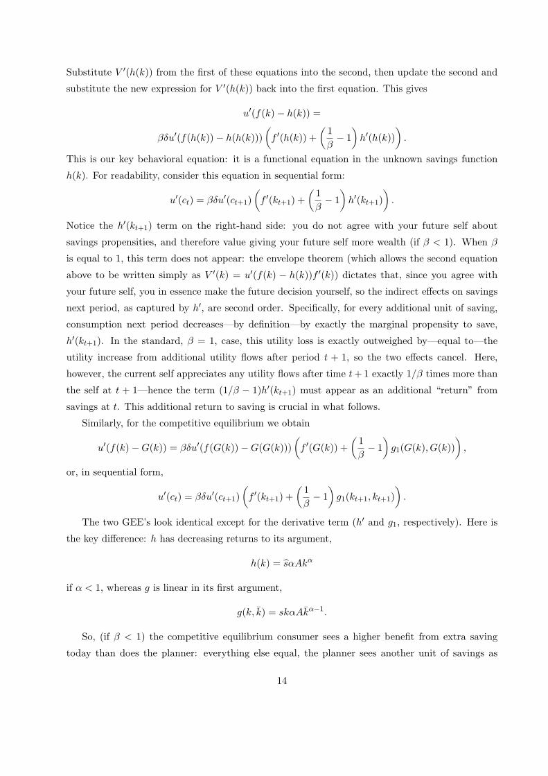
Substitute V ′(h(k)) from the first of these equations into the second, then update the second and
substitute the new expression for V ′(h(k)) back into the first equation. This gives
u′(f(k)− h(k)) =
βδu′(f(h(k))− h(h(k)))(f ′(h(k)) +
(1β− 1
)h′(h(k))
).
This is our key behavioral equation: it is a functional equation in the unknown savings function
h(k). For readability, consider this equation in sequential form:
u′(ct) = βδu′(ct+1)(f ′(kt+1) +
(1β− 1
)h′(kt+1)
).
Notice the h′(kt+1) term on the right-hand side: you do not agree with your future self about
savings propensities, and therefore value giving your future self more wealth (if β < 1). When β
is equal to 1, this term does not appear: the envelope theorem (which allows the second equation
above to be written simply as V ′(k) = u′(f(k) − h(k))f ′(k)) dictates that, since you agree with
your future self, you in essence make the future decision yourself, so the indirect effects on savings
next period, as captured by h′, are second order. Specifically, for every additional unit of saving,
consumption next period decreases—by definition—by exactly the marginal propensity to save,
h′(kt+1). In the standard, β = 1, case, this utility loss is exactly outweighed by—equal to—the
utility increase from additional utility flows after period t + 1, so the two effects cancel. Here,
however, the current self appreciates any utility flows after time t+ 1 exactly 1/β times more than
the self at t + 1—hence the term (1/β − 1)h′(kt+1) must appear as an additional “return” from
savings at t. This additional return to saving is crucial in what follows.
Similarly, for the competitive equilibrium we obtain
u′(f(k)−G(k)) = βδu′(f(G(k))−G(G(k)))(f ′(G(k)) +
(1β− 1
)g1(G(k), G(k))
),
or, in sequential form,
u′(ct) = βδu′(ct+1)(f ′(kt+1) +
(1β− 1
)g1(kt+1, kt+1)
).
The two GEE’s look identical except for the derivative term (h′ and g1, respectively). Here is
the key difference: h has decreasing returns to its argument,
h(k) = sαAkα
if α < 1, whereas g is linear in its first argument,
g(k, k) = skαAkα−1.
So, (if β < 1) the competitive equilibrium consumer sees a higher benefit from extra saving
today than does the planner: everything else equal, the planner sees another unit of savings as
14
yielding a smaller increase in future savings than does the competitive-equilibrium consumer. This
makes the competitive agent save more than the planner, because the future selves are undersaving
and extra future saving is now a good thing. The argument works for β > 1 as well. Then, the
planner saves more than the competitive equilibrium, which saves too much. An extra saved unit
increases future savings more as perceived by the consumer than as perceived by the planner. As
a result, the consumer saves less than the planner since extra future savings is now a bad thing.
Behind these arguments is the main difference between a planner and a competitive individual:
the planner understands that he affects the “prices”, that is, the return to savings, whereas a price-
taker does not. This implies that the marginal propensity to save for the planner is decreasing,
whereas it is constant for the competitive agent. This is the key difference behind the planner’s
and the competitive agent’s decision rules.
4.4 Utility comparisons for other agents
One might take the view that the consumer’s future selves, and their different preferences, ought
to be respected and taken separately into account in the comparison between the two allocations
above. Suppose, therefore, that we evaluate the utility of the self next in line as he perceives it.
Would he prefer the competitive or the central planning allocation?
It is clear from the arguments in the preceding section that, if the next self were given the same
amount of capital to start with in both situations, then he would prefer the competitive allocation;
it provides higher savings at all times, which is perceived as better (if β < 1). However, capital is
not constant across the two allocations. Depending on the value of β, it is either higher or lower.
If β < 1, it is higher, and the competitive equilibrium dominates, not only in the next period,
but in all future periods as well. This is the case most commonly emphasized in the literature on
time-inconsistent preferences. In this case, therefore, the competitive equilibrium allocation Pareto
dominates the central planning allocation. If, on the other hand, β > 1, there is an effect in favor
of the central planning allocation for all future selves, and the net result is not clear.
4.5 Robustness: some examples
The savings and utility comparisons above across the centralized and decentralized economies use
a particular parameterization. We will now briefly discuss a slightly broader class of economies—
one with isoelastic utility and less than full depreciation of capital, in which case no closed-form
solution can be obtained. First, we compare steady-state capital stocks; it is possible to show that
the planning outcome always gives a lower long-run capital stock.10 Second, we consider utility:
we compare the current-self utility at a decentralized steady state to that given by the planning
outcome starting from the same capital stock as in the decentralized steady state.
15
4.5.1 Steady states
Recursive competitive equilibria for the present class of economies can be characterized by two
functions, λ(k) and µ(k), whenever utility is isoelastic (that is, independently of the production
structure). In particular, Hercowitz and Krusell [7] showed that the policy function of the individual
satisfies
g(k, k) = µ(k) + λ(k)k.
The shape of the two unknown functions depends on the specifics of preferences and technology.11
That is, savings are affine in the individual’s wealth with coefficients that depend only on aggre-
gate variables—an aggregation result that is expected given isoelastic utility. Moreover, at the
steady-state equilibrium capital stock, kE , the functions satisfy µ(kE) = 0 and λ(kE) = 1: the
“permanent income hypothesis” holds (any increase in initial capital is saved forever, leaving a
constant increase in consumption equal to the return on the added capital). This means that the
competitive equilibrium steady state must satisfy
1 = βδ
(f ′(kE) +
(1β− 1
)g1(kE , kE)
)= βδ
(f ′(kE) +
1β− 1
),
where the last equality follows from the condition g1(kE , kE) = λ(kE) = 1 just stated. This delivers
kE = (f ′)−1(
1− δ(1− β)βδ
).
We note that the steady-state capital stock is independent of the curvature of the utility function,
as in the model where β = 1.12
The steady state for the planning problem cannot be derived analytically; the value of the
constant capital stock, kP , satisfies
1 = βδ
(f ′(kP ) +
(1β− 1
)h′(kP )
),
but h′(kP ) has no closed-form expression. However, we know that it has to be less than 1 for the
steady state to be stable (which we regard as a minimal requirement for being interested in a steady
state). Thus, assuming that the steady state is stable, and following the same algebra as above, we
see that kP has to satisfy
kP = (f ′)−1
(1− δ(1− β)h′(kP )
βδ
).
Because of stability,1− δ(1− β)h′(kP )
βδ>
1− δ(1− β)βδ
.
Thus, whenever (f ′)−1 is strictly decreasing (which we also assume, given the neoclassical focus
here), kP < kE must hold.
16
4.5.2 Numerical solution of the planner’s problem
For specific utility comparisons, we need to use numerical methods, which requires us to specify
a production technology and give values to parameters. Before proceeding to results, we need
to comment on the numerical methods that we use. There are two reasons for this: (i) we have
developed new methods, since standard methods fail; and (ii) these new methods are likely to
be useful also in other applications where the decision maker’s commitment solution is not time-
consistent and a time-consistent solution is sought, such as in many macroeconomic problems of
optimal policy determination.
In contrast to the standard model, numerically solving the present model—even in partial
equilibrium, and even when β is very close to 1—can be a daunting task, because many standard
algorithms fail.13 Techniques relying on value-function iteration fail to converge and instead tend
to cycle, while Euler equation methods tend to generate multiple solutions. We strongly suspect
that these problems have their roots in the indeterminacy finding of Krusell and Smith [11]: with
an infinite set of Markov solutions, any numerical routine not relying on specific properties of the
solution will have severe difficulties.14
Our new method can be viewed in some respects as a variation on the regular perturbation
method described in Chapter 13 of Judd [8]. Specifically, it is based on repeated differentiation of
the GEE, and therefore assumes that the policy function is differentiable many times. As a first
step towards understanding our algorithm, notice that the GEE, evaluated at the steady state,
contains, in effect, two unknowns: the level of the policy function, h(kP ) = kP , and its derivative,
h′(kP ). Thus the GEE, evaluated at the steady state, can be viewed as a single equation in these
two unknowns. To generate another equation, one can proceed as in Judd [8]: differentiate the
GEE, which holds for all values of the state variable, and evaluate it at the steady state. However,
this equation now in addition contains another unknown, h′′(kP ). In a first-order approximation
to the policy function, we set h′′(kP ) = 0, thereby giving us two equations in the two unknowns kPand h′(kP ).
To compute a second-order approximation to the policy function, we can differentiate the GEE
again, yielding an equation that now contains h′′′(kP ). By setting this third derivative equal to
0, we obtain three equations in the three unknowns kP , h′(kP ), and h′′(kP ). Evidently, every
differentiation of the GEE produces an additional equation but also an additional unknown, which
we set to 0 in order to compute an approximation of a given order.
The fact that an additional unknown appears when we differentiate the GEE means that ap-
plying the regular perturbation method to this problem is computationally more demanding than
applying it to the standard growth model. For the standard model, the steady-state capital stock
can be computed directly from the Euler equation without knowing anything about the derivatives
17
of the policy function. Moreover, successive differentiations of the Euler equation simply yield one
additional unknown, namely, the next higher-order derivative of the policy function, evaluated at
the steady state. Consequently, in the standard model, one can compute the sequence of derivatives
of the policy function iteratively. In our model, by contrast, we must solve simultaneously both for
the steady state and the derivatives of the policy function.
To solve for the steady state and the derivatives of the policy function at the steady state, we
use an algorithm that is inspired by the “perturbation” ideas described above, but which differs
in the details of implementation. Specifically, we let the policy function be approximated by a
polynomial of order n − 1 (with the logarithm of the capital stock as the state variable). The
goal of the algorithm is to choose the n coefficients of this polynomial, together with the steady
state, to satisfy n+ 1 restrictions. One of these restrictions is that the steady state be a stationary
point of the approximate decision rule. The remaining n restrictions are that the GEE and its first
n − 1 derivatives equal 0 when evaluated at the steady state. Thus, we are in effect choosing the
level of the decision rule and its first n derivatives to solve the set of equations generated by the
perturbation method described above. Appendix 2 describes our algorithm in much greater detail.
4.5.3 Utility comparisons
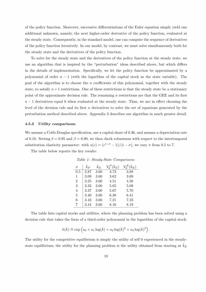
We assume a Cobb-Douglas specification, use a capital share of 0.36, and assume a depreciation rate
of 0.10. Setting δ = 0.95 and β = 0.90, we then check robustness with respect to the intertemporal
substitution elasticity parameter: with u(c) = (c1−σ − 1)/(1− σ), we vary σ from 0.5 to 7.
The table below reports the key results:
Table 1: Steady-State Comparisons
σ kP kE V P0 (kE) V E
0 (kE)0.5 2.87 3.60 3.73 3.881 3.09 3.60 3.62 3.692 3.25 3.60 4.51 4.563 3.33 3.60 5.05 5.094 3.37 3.60 5.67 5.705 3.40 3.60 6.38 6.416 3.43 3.60 7.21 7.237 3.44 3.60 8.16 8.19
The table lists capital stocks and utilities, where the planning problem has been solved using a
decision rule that takes the form of a third-order polynomial in the logarithm of the capital stock:
h(k) ∼= exp(a0 + a1 log(k) + a2 log(k)2 + a3 log(k)3
).
The utility for the competitive equilibrium is simply the utility of self 0 experienced in the steady-
state equilibrium; the utility for the planning problem is the utility obtained from starting at kE
18

and then converging to the planning steady state kP . We see from the table that, as shown in
the previous section, the planning steady state is always below the competitive steady state and
that the former depends on the curvature of u, whereas the latter does not. We also see that the
planning steady state becomes closer to the equilibrium steady state as the curvature increases: it
is well known that increased curvature leads to slower convergence, that is, to a higher derivative
of the decision rule at steady state, which we know from the above section makes the steady states
closer. Utility is always higher in equilibrium than in the planning solution. That is, our theoretical
findings above is robust at least to the variations presented here.
5 Policy Analysis
The planning problem in the previous section can perhaps be viewed as artificial. In this section
we consider a government with taxation abilities. There are no government expenditures and we
impose budget balance; moreover, we assume that the government is benevolent in that it is the
representative of the consumer. As the planner, the government cannot commit its future self:
future tax rates are set by future governments, and future governments have different preferences,
as they are representatives for the futures selves of the consumer.
Assume that the government can tax income and investment at proportional rates τy and τi,
respectively. The first of these is essentially a lump-sum tax in this model, since income and
substitution effects cancel with logarithmic utility. The investment tax, on the other hand, is
distortionary.
We first consider the full commitment case for illustration. We then turn to time-consistent
taxation. Time-consistent taxation in this model leads to taxes which are constant over time (as
are savings rates).
5.1 Full commitment to future taxes
Since the consumer’s future selves are undersaving from the perspective of the current self, the
government will want to subsidize investment in all future periods. Given the stationarity of the
problem and the log/Cobb-Douglas assumptions, these rates will be constant and given by
τ ′i =(1− δ) (β − 1)
1− δ + δβ − αδβand τ ′y =
αδ (1− δ) (1− β)1− δ + δβ − αδβ
.
These tax rates for future periods will give a savings rate of δ for these periods. For the current
period, the government sets the tax rates
τi =δ (1− α) (1− β)
1− αδ − δ (1− α) (1− β)and τy =
αδ2β (1− α) (1− β)αδ2β (1− α) (1− β)− (1− αδ) (1− δ (1− β))
.
19
This gives a savings rate of δβ1−αδ(1−β) for the current period. This tax sequence generated by fully
committed governments is not time-consistent. This creates incentives for future governments to
deviate. We now move on to time-consistent taxation.
5.2 No commitment: time-consistent policy
We define a subgame-perfect Markov equilibrium for the government problem. This definition
parallels the definition of subgame-perfect Markov equilibria: a tax function describes the tax
outcome as a function of the aggregate state, and to support this tax function it is necessary
to consider one-period deviations from the equilibrium path.15 The competitive equilibrium is
defined as above for given taxes. Before we go through the definition of the time-consistent policy
equilibrium, let us point out that taxes in this equilibrium will be constant, due to our special
parametric assumptions. To support them as being constant, however, it is necessary to formally
verify all the conditions of a subgame-perfect Markov equilibrium.
Definition 2 A time-consistent policy equilibrium is defined in several parts; the elements are
listed below.
First, the behavior on the equilibrium path (“outcomes”) are as follows:
• Tax outcomes are given by τ(k)
=(τy(k), τi(k)).
• Given this tax function, the law of motion for aggregate capital is given by G(k).
• Given the tax function and the law of motion for aggregate capital, the individual’s decision
rule is given by g(k, k
)Second, the one-period deviations to tax rates τ = (τy, τi) for the current period, with future
taxes given by the tax outcome functions evaluated at the capital stocks implied by the current tax
rates and the implied capital accumulation, are given by the following:
• G(k, τ
)describes the law of motion for aggregate capital for the one-period deviation.
• g(k, k, τ
)describes the individual’s decision rule for the one-period deviation.
Third, we have competitive pricing functions r(k) and w(k) (equal to the marginal products off
the aggregate production function).
These equilibrium elements have to satisfy:
20
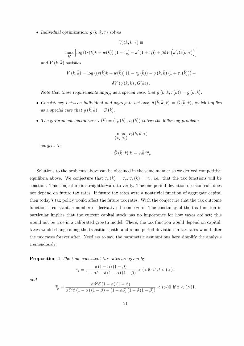
• Individual optimization: g(k, k, τ
)solves
V0(k, k, τ) ≡
maxk′
[log
((r(k)k + w(k)
)(1− τy)− k′ (1 + τi)
)+ βδV
(k′, G(k, τ)
)]and V
(k, k
)satisfies
V(k, k
)= log
((r(k)k + w(k)
) (1− τy
(k))− g
(k, k
) (1 + τi
(k)))
+
δV(g(k, k
), G(k)
).
Note that these requirements imply, as a special case, that g(k, k, τ(k)
)= g
(k, k
).
• Consistency between individual and aggregate actions: g(k, k, τ
)= G
(k, τ
), which implies
as a special case that g(k, k
)= G
(k).
• The government maximizes: τ(k)
=(τy(k), τi(k))
solves the following problem:
max(τy, τi)
V0(k, k, τ)
subject to:
−G(k, τ
)τi = Akατy.
Solutions to the problems above can be obtained in the same manner as we derived competitive
equilibria above. We conjecture that τy(k)
= τy, τi(k)
= τi, i.e., that the tax functions will be
constant. This conjecture is straightforward to verify. The one-period deviation decision rule does
not depend on future tax rates. If future tax rates were a nontrivial function of aggregate capital
then today’s tax policy would affect the future tax rates. With the conjecture that the tax outcome
function is constant, a number of derivatives become zero. The constancy of the tax function in
particular implies that the current capital stock has no importance for how taxes are set; this
would not be true in a calibrated growth model. There, the tax function would depend on capital,
taxes would change along the transition path, and a one-period deviation in tax rates would alter
the tax rates forever after. Needless to say, the parametric assumptions here simplify the analysis
tremendously.
Proposition 4 The time-consistent tax rates are given by
τi =δ (1− α) (1− β)
1− αδ − δ (1− α) (1− β)> (<)0 if β < (>)1
and
τy =αδ2β (1− α) (1− β)
αδ2β (1− α) (1− β)− (1− αδ) (1− δ (1− β))< (>)0 if β < (>)1.
21
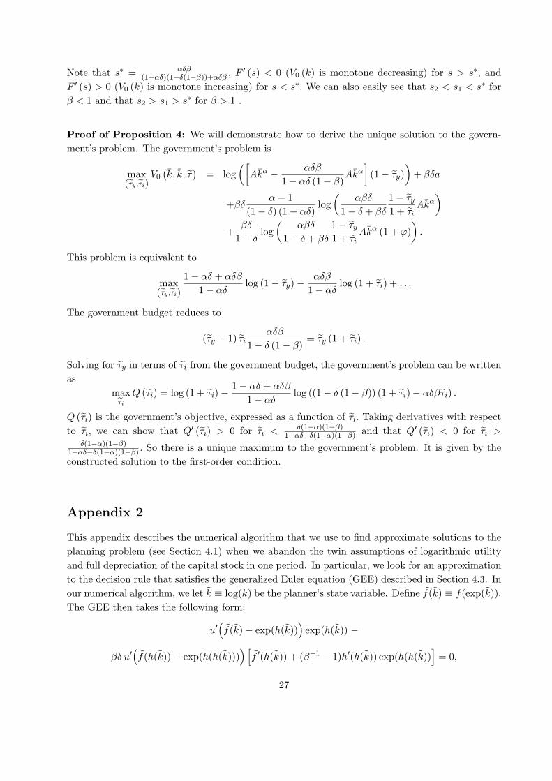
Proof: See Appendix 1.
It is straightforward to verify that the time-consistent tax rates, perhaps not surprisingly, re-
produce the allocations that solve the planner’s game: the government has enough instruments to
manipulate current decisions freely, and so chooses the same outcome as if it were a central planner.
As a positive theory of taxation, the model implies
τi > (<) 0 if β < (>) 1
and
τy < (>) 0 if β < (>) 1.
That is, we have positive tax rates on investment when β < 1. The social planner saves much too
little (less than the laissez-faire equilibrium) and so wants to move the equilibrium in the “wrong
direction”.
6 Summary and concluding remarks
We have studied the performance of the market mechanism relative to a mechanism with a benevo-
lent and potentially active government in what we believe is an interesting new case for economists
to study: an economy where consumers have time-inconsistent preferences. Our analysis comes out
surprisingly strongly in favor of laissez-faire; an initial reader of the literature on time-inconsistent
preferences may get the impression that the consumer needs help and that the government can
provide the help. We argue here that this is really only true if the government, or social planner,
can help alleviate the commitment problem in a direct way, or indirectly by being able to commit
to future tax rates. Further, under the assumption that the government cannot do anything about
the commitment problem, we should strictly prefer laissez-faire. It would be important not to have
a government that can tax. Although are goal here is not to send a libertarian message, the results
here may perhaps be interpreted as a caution against tax policy activism: taxes should not be used
to try to correct problems whose underlying cause is a lack of commitment to which the government
is also subject.
Could the government provide commitment mechanisms to aid consumers with time-inconsistent
preferences? To the extent that it could close short-term credit markets in the future, in effect
“creating illiquidity” in the future, then it should, ceteris paribus. However, we argued that ex
post—when the future arrives—it will be in everybody’s interest not to close the markets, and it
is unclear how a commitment mechanism for the closing of markets in the future could be cre-
ated. Moreover, providing illiquidity by offering assets such as the 401(k)—with penalty for early
22
withdrawals—might be helpful, but only if other restrictions on trading/borrowing are simultane-
ously and credibly put in place. In general, commitment is needed for consumption, and it is not
enough to provide assets which are illiquid. Therefore, we take the present analysis as an entirely
relevant case.
We found that our tax policy analysis bears resemblance to the “rules vs. discretion” literature.
Our government here is benevolent—a samaritan—but it cannot help but adopt policies that are not
good. What is the solution to our samaritan’s dilemma? Short of some form of commitment, there
is no solution. Along the lines of Rogoff’s [20] suggestion in the monetary literature of electing a
“conservative” to head the central bank in the future, one could imagine in our context electing, for
an extended period, a planner who places independent weight on utility as perceived by the future
selves of the consumer. With appropriate such weights—they have to be large enough—outcomes
could be improved for all selves. However, the mere idea of being able to elect a planner for the
future, or tomorrow’s central banker, is one of commitment. Absent institutional rules (that are
set in stone) it would then be difficult to explain why it is possible to commit to a future decision
maker but not to future policies.
One weakness of the present approach to representing the preference reversals documented in
the experimental psychology literature is that it makes a rather drastic conceptual departure from
standard Arrow-Debreu analysis. In particular, it does not build up from axioms of choice for
the individual. What would seem to be appropriately captured by an optimization problem—the
consumer’s observed behavior—is instead modelled here as the solution to a dynamic game. As
such, all the usual problems of (dynamic) game theory appear; for example, indeterminacy of
equilibrium is the rule rather than the exception. We “resolve” this problem by focusing on the
limit of the equilibria of finite-horizon economies. Several comments are in order.
First, many practical applications (such as those considered in Laibson’s papers) do have a
finite horizon, and our results are directly relevant here: although we do not explicitly consider
finite-horizon problems, our results apply if the time horizon is long enough, and they are likely
to carry over also to short horizons (e.g., it is straightforward to derive results for a three-period
model).
Second, although we do not find the other equilibria uninteresting, we find it particularly instruc-
tive to study equilibria without the “reputation” effects that typically underly the indeterminacy
of equilibria in dynamic games. In particular, the economic incentives upon which we focus in
this paper will be present whether or not there are additional incentives arising from punishment
schemes. In other words, the “reputation-free” equilibrium is very interesting in itself here, unlike
in, say, the repeated Prisoner’s Dilemma model.
Third, we show that there are basic economic forces leading the decentralized (laissez-faire)
equilibrium to perform well in our model. Although there surely exist decentralized equilibria with
23
reputation effects that perform worse than specific planning equilibria (and vice versa), we do not
have an insight as to whether the consideration of reputation-based equilibria would systematically
alter these comparisons.
Fourth and finally, it is useful for our welfare comparisons that the equilibria upon which we
focus here (i.e., those that are limits of finite-horizon equilibria) are unique. Under particular
assumptions about preferences and technology, such equilibria are unique. Moreover, our computa-
tional experiments that generalize the utility function and consider less than full depreciation show
no indication of multiplicity. Finally, we suspect that it is not an easy task to generate examples
with multiple solutions to finite-horizon games in the context of the neoclassical growth model with
quasi-geometric discounting.
An alternative approach to the one we follow here, and one which may ultimately turn out to
be more fruitful, is undertaken in a set of papers by Gul and Pesendorfer [4,5]. These authors use
decision theory, based on axioms over sets of consumption bundles, and arrive at recursive (time-
consistent) preference representations of consumer behavior when “temptation” and “self-control”
are represented axiomatically. In a related paper (Krusell, Kuruscu, and Smith [10]), we are
considering the effects of policy on equilibrium allocations and welfare when there is “temptation”
and “self-control”, as in Gul and Pesendorfer’s framework.
24
REFERENCES
1. G. Ainslie, “Picoeconomics”, Cambridge University Press, Cambridge, 1992.2. R. Barro, “Ramsey Meets Laibson in the Neoclassical Growth Model”, Quarterly Journal ofEconomics 114 (1999), 1125–1152.3. D. B. Bernheim, D. Ray, and S. Yeltekin, “Self-Control, Saving, and the Low Asset Trap”,Manuscript, 1999.4. F. Gul and W. Pesendorfer, “Temptation and Self-Control”, Manuscript, Princeton University,2000 (forthcoming in Econometrica).5. F. Gul and W. Pesendorfer, “Self-Control and the Theory of Consumption”, Manuscript, Prince-ton University, 2000.6. C. Harris and D. Laibson, “Dynamic Choices of Hyperbolic Consumers”, Manuscript, 2000(forthcoming in Econometrica).7. Z. Hercowitz and P. Krusell, “Overheating”, Manuscript, 2001.8. K. L. Judd, “Numerical Methods in Economics”, MIT Press, Cambridge, 1998.9. P. Krusell and J.-V. Rıos-Rull, “On the Size of U.S. Government: Political Economy in theNeoclassical Growth Model”, American Economic Review 89 (1999), 1156–1181.10. P. Krusell, B. Kuruscu, and A. A. Smith, Jr. “Temptation and Taxation”, Manuscript, 2001.11. P. Krusell and A. A. Smith, Jr. “Consumption-Savings Decisions with Quasi-GeometricDiscounting”, Manuscript, 2000.12. F. Kydland and E. C. Prescott, “Rules Rather than Discretion: The Inconsistency of OptimalPlans”, Journal of Political Economy 85 (1977), 473–491.13. D. Laibson, “Self-Control and Saving”, Ph.D. thesis, MIT, 1994.14. D. Laibson, “Hyperbolic Discount Functions, Undersaving, and Savings Policy”, NBER Work-ing Paper 5635, 1996.15. D. Laibson, “Hyperbolic Discount Functions and Time Preference Heterogeneity”, Manuscript,1997.16. D. Laibson, A. Repetto, and J. Tobacman, “Self-Control and Saving for Retirement”, BrookingsPapers on Economic Activity No 1 (1998), 91–196.17. E. D. O’Donoghue and M. Rabin, “Doing It Now or Doing It Later”, American EconomicReview 89 1999, 103–124.18. E. Phelps and R. A. Pollak, “On Second-best National Saving and Game-equilibrium Growth”,Review of Economic Studies 35 (1968), 185–199.19. W. H. Press, B. P. Flannery, S. A. Teukolski, and W. T. Vetterling, Numerical Recipes: TheArt of Scientific Computing , Cambridge University Press, Cambridge, 1989.20. K. Rogoff, “The Optimal Degree of Commitment to an Intermediate Monetary Target”, Quar-terly Journal of Economics 100 (1985), 1169–1190.21. R. H. Strotz, “Myopia and Inconsistency in Dynamic Utility Maximization”, Review of Eco-nomic Studies 23 (1956), 165–180.
25
Appendix 1
Proof of Proposition 1: The proof follows by using the guess for the value function, V(k, k
)=
a+b log k+c log(k + ϕk
), and the guess for the law of motion for aggregate capital, G
(k)
= sαAkα.16 Given these guesses we can solve the current self’s problem to obtain g
(k, k
)= βδc
1+βδc (rk + w)−ϕk′
1+βδc . Using this decision rule we can verify the guess for the value function and obtain ϕ = 1−αα(1−s)
, b = α−1(1−δ)(1−αδ) , and c = 1
1−δ . Inserting ϕ = 1−αα(1−s) into the individual decision rules and setting
g(k, k
)= G
(k)
(which has to hold in competitive equilibrium), we obtain s = δβ1−δ(1−β) . This gives
ϕ = (1−α)(1−δ(1−β))α(1−δ) . Substituting these constants into the agent’s decision rule, we obtain g
(k, k
)and G
(k).
Proof of Proposition 3: The proof proceeds as follows: first we derive the value function of thecurrent self, V0 (k) , given a general law of motion of type k′ = sAkα. We thus obtain a function ofs. We then evaluate this value function at s1 = αδβ
1−δ(1−β) and at s2 = αδβ1−αδ(1−β) .
Let us first derive V (k) . For the given law of motion for capital, consumption will be given byc = (1− s)Akα. Then we can write V (k) as
V (k) = log ((1− s)Akα) + δ log((1− s)Ak′α
)+ δ2 log
((1− s)Ak′′α
)+ . . . .
Inserting the law of motion for the capital we obtain
V (k) =1− αδ
(1− αδ) (1− δ)log (1− s) +
αδ
(1− αδ) (1− δ)log s
+α
(1− αδ)log k +
1(1− αδ) (1− δ)
logA.
V0 (k) is now given by
V0 (k) = log ((1− s)Akα) + βδV (sAkα)
= log ((1− s)Akα) +
βδ
[1−αδ
(1−αδ)(1−δ) log (1− s) + αδ(1−αδ)(1−δ) log s
+ α(1−αδ) log (sAkα) + 1
(1−αδ)(1−δ) logA
]
=1− δ (1− β)
1− δlog (1− s) +
αδβ
(1− αδ) (1− δ)log s+ . . . .
To evaluate V0 (k) at s1 and s2, we proceed as follows. We first show that there is a uniques∗ that maximizes V0 (k) , by showing that V0 (k) is monotone increasing in s for s < s∗ andmonotone decreasing for s > s∗. We then complete the proof by showing that s2 < s1 < s∗ forβ < 1 , and s2 > s1 > s∗ for β > 1 . To do this, first let us look at the function F (s) =(1− δ (1− β)) log (1− s) + αδβ
1−αδ log s.
F ′ (s) = −(1− δ (1− β))1− s
+αδβ
(1− αδ) s
= − [(1− αδ) (1− δ (1− β)) + αδβ] s− αδβ
s (1− s) (1− αδ)
26
Note that s∗ = αδβ(1−αδ)(1−δ(1−β))+αδβ , F
′ (s) < 0 (V0 (k) is monotone decreasing) for s > s∗, andF ′ (s) > 0 (V0 (k) is monotone increasing) for s < s∗. We can also easily see that s2 < s1 < s∗ forβ < 1 and that s2 > s1 > s∗ for β > 1 .
Proof of Proposition 4: We will demonstrate how to derive the unique solution to the govern-ment’s problem. The government’s problem is
max(τy ,τi)
V0(k, k, τ
)= log
([Akα − αδβ
1− αδ (1− β)Akα
](1− τy)
)+ βδa
+βδα− 1
(1− δ) (1− αδ)log
(αβδ
1− δ + βδ
1− τy1 + τi
Akα)
+βδ
1− δlog
(αβδ
1− δ + βδ
1− τy1 + τi
Akα (1 + ϕ)).
This problem is equivalent to
max(τy ,τi)
1− αδ + αδβ
1− αδlog (1− τy)−
αδβ
1− αδlog (1 + τi) + . . .
The government budget reduces to
(τy − 1) τiαδβ
1− δ (1− β)= τy (1 + τi) .
Solving for τy in terms of τi from the government budget, the government’s problem can be writtenas
maxτi
Q (τi) = log (1 + τi)−1− αδ + αδβ
1− αδlog ((1− δ (1− β)) (1 + τi)− αδβτi) .
Q (τi) is the government’s objective, expressed as a function of τi. Taking derivatives with respectto τi, we can show that Q′ (τi) > 0 for τi <
δ(1−α)(1−β)1−αδ−δ(1−α)(1−β) and that Q′ (τi) < 0 for τi >
δ(1−α)(1−β)1−αδ−δ(1−α)(1−β) . So there is a unique maximum to the government’s problem. It is given by theconstructed solution to the first-order condition.
Appendix 2
This appendix describes the numerical algorithm that we use to find approximate solutions to theplanning problem (see Section 4.1) when we abandon the twin assumptions of logarithmic utilityand full depreciation of the capital stock in one period. In particular, we look for an approximationto the decision rule that satisfies the generalized Euler equation (GEE) described in Section 4.3. Inour numerical algorithm, we let k ≡ log(k) be the planner’s state variable. Define f(k) ≡ f(exp(k)).The GEE then takes the following form:
u′(f(k)− exp(h(k))
)exp(h(k)) −
βδ u′(f(h(k))− exp(h(h(k)))
) [f ′(h(k)) + (β−1 − 1)h′(h(k)) exp(h(h(k))
]= 0,
27
where h is the planner’s decision rule (in logs). Given h, the GEE can be written more compactly asH(k) = 0. Let H(m) denote the mth derivative of H. Since the GEE holds for all k, H(m)(k) = 0for all m and all k. We use this fact in our numerical algorithm to define restrictions that anapproximate solution to the GEE must satisfy.
Let hψ be an approximation to the unknown decision rule h characterized by an n-dimensionalvector of parameters ψ. For example, h could be a polynomial of order n − 1, with ψ being a setof n coefficients. The basic idea of our numerical algorithm is to choose the coefficients ψ so thatH and its first n− 1 derivatives are equal to zero when evaluated at a particular value of k.
Specifically, let Hψ be the value of the left-hand side of the GEE when h is replaced bythe approximate decision rule hψ. We choose ψ to solve the n equations H(m)
ψ (k∗) = 0, m =
0, 1, 2, . . . , n − 1, where H(m)ψ is the mth derivative of Hψ and k∗ is an arbitrarily chosen point in
the state space.Since we are typically interested in dynamic behavior near the steady-state capital stock kss,
we would like to evaluate Hψ and its derivatives at kss (but note that the algorithm is well-definedand works well in practice even if we evaluate Hψ and its derivatives at an arbitrary point in thestate space). Unlike in the standard model (where β = 1), we cannot solve for kss without solvingsimultaneously for the equilibrium decision rule (since the derivative of the decision rule appears inthe GEE). We therefore solve for the decision rule coefficients ψ and the steady-state capital stockkss at the same time, with kss being pinned down by the requirement that kss − hψ(kss) = 0. Insum, our algorithm boils down to the solution of n+ 1 equations in the n+ 1 unknowns ψ and kss.
We have implemented this algorithm using polynomial decision rules up to order 3. We definehψ using ordinary polynomials: hψ(k) =
∑n−1i=0 aik
i. We find that the numerical results changeonly to a small degree when increasing the order of the polynomial from 2 to 3. In order to avoidcollinearity problems, a higher-order implementation of the algorithm would probably require theuse of polynomials defined in terms of a set of orthogonal polynomials (such as the Chebyshevpolynomials).
To solve the n+ 1 equations, we use the simplex algorithm as described in Chapter 10 of Presset al. [19]. Specifically, we choose ψ and kss to minimize the objective function
n−1∑i=0
(H
(i)ψ (kss)
)2+(kss − hψ(kss)
)2.
In all of the cases that we tried, we were able to find values for ψ and kss that set this objectivefunction equal to 0. Although we could use a variety of other methods to solve for ψ and kss, thismethod is reasonably robust and is sufficiently fast.
The simplex algorithm requires an initial simplex consisting of n + 2 points (ψ, kss) ∈ Rn+1.We let one of these points correspond to a parameterization of the model economy for which wehave a closed-form solution (for example, logarithmic utility and full depreciation of the capitalstock in one period). We choose the remaining points in the simplex to be random perturbationsof this point. We then solve the n+ 1 equations for a parameterization of the model economy thatis “close” to the parameterization with the closed-form solution. This solution serves in turn asone of the points in the initial simplex when we perturb the model economy’s parameters again.
28

Although the required derivatives could be calculated analytically, we calculate them numeri-cally using the following “two-sided” finite-difference formulas:
H(1)ψ (k) ≈
Hψ
((1 + ε1)k
)− Hψ
((1− ε1)k
)2ε1k
H(2)ψ (k) ≈
Hψ
((1 + 2ε2)k
)− 2Hψ(k) + Hψ
((1− 2ε2)k
)(2ε2k)2
H(3)ψ (k) ≈
Hψ
((1 + 3ε3)k
)− 3Hψ
((1 + ε3)k
)+ 3Hψ
((1− ε3)k
)− Hψ
((1− 3ε3)k
)(2ε3k)3
,
with εi = 10−6/i for i = 1, 2, 3.
29

Notes
1The term quasi-hyperbolic commonly used in the recent literature—see, e.g., Laibson [11]—refers to the use of a quasi-geometric discounting function in order to approximate a (generalized)hyperbolic function.
2Indeed, we look precisely at the class of discounting functions referred to as quasi-hyperbolic.As indicated in the previous footnote, the correct mathematical term for these functions is quasi-geometric; they are quasi-hyperbolic only in the sense that, for certain parameter values, theyresemble a generalized hyperbolic function.
3The argument is parallel when the time-inconsistency takes the form of excessive short-runpatience.
4The term quasi-hyperbolic is used in the literature as referring to the same preference setupeven though, mathematically, hyperbolic functions take an entirely different form. The reason forthe use of the term quasi-hyperbolic is that, for certain parameter values—see Figure 1 below—thediscounting function resembles a (generalized) hyperbola. Here, we are interested in the entire classof quasi-geometric preferences.
5One would then, for example, assume that the disagreement between current self and the self kperiods later disagree not only on the value of date t+ k consumption relative to other goods, buton the relative value of date t+k+1 consumption as well. This extension would simply require theintroduction of “another β”. Successive introductions of more βs would then relax the geometricframework more and more.
6One could argue that commitment mechanisms are more likely to occur within tight socialgroups/families. Social networks would then potentially play an important role in accumulationdecisions.
7Others, such as O’Donoghue and Rabin [17], in addition consider the possibility that theconsumer does not realize that his preferences will change.
8We discuss reasons for our refinement strategy in Section 6.
9We briefly discuss implications of having meta-planners below.
10Throughout this section, we assume that β < 1.
11They satisfy a pair of functional equations.
12This fact was noted in Barro [2].
13This is not a new observation; see Laibson, Repetto, and Tobacman [16].
14Two comments are in order. First, the fact that we are searching for a continuous solution heremight seem enough for ruling out the large set of solutions uncovered in Krusell and Smith [11], sincethe latter are discontinuous by construction. However, the discontinuities are countable in numberand seem hard to detect with global methods. Second, one might think that backwards solution,given a finite-horizon problem as in Laibson, Repetto, and Tobacman [16], would work. However,the horizon does not have to be very long for a multitude of “near-solutions” to cause problems for
30

standard algorithms: the indeterminacy result implies existence of these near-solutions.
15For a definition in the context of a typical growth model, see Krusell and Rıos-Rull [9].
16Where does this guess come from? ϕk is actually equal to discounted value of lifetime wages(discounted to time −1 in this formulation): w
r + w′
rr′ + w′′
rr′r′′ + ..... If we use G(k)
= sαAkα andplug it into the discounted sum, we obtain ϕ = 1−α
α(1−s) .
31