Icarus 205 (2010) 638–657

Contents lists available at ScienceDirect

Icarus

journal homepage: www.elsevier .com/ locate/ icarus

Equilibrium shapes of rubble-pile binaries: The Darwin ellipsoidsfor gravitationally held granular aggregates

Ishan Sharma *

Department of Mechanical Engineering, IIT Kanpur, Kanpur 208016, India

a r t i c l e i n f o a b s t r a c t

Article history:Received 4 March 2009Revised 31 July 2009Accepted 8 August 2009Available online 3 September 2009

Keywords:Asteroids, RotationAsteroids, DynamicsGeophysicsNear-Earth objects

0019-1035/$ - see front matter � 2009 Elsevier Inc. Adoi:10.1016/j.icarus.2009.08.018

* Fax: +91 512 259 7408.E-mail address: ishans@iitk.ac.in.

Binaries are in vogue; many minor-planets like asteroids are being found to be binary or contact-binarysystems. Even ternaries like 87 Sylvia have been discovered. The densities of these binaries are often esti-mated to be very low, and this, along with suspected accretionary origins, hints at a rubble interior. As inthe case of fluid objects, a rubble-pile is unable to sustain all manners of spin, self-gravitation, and tidalinteractions. This motivates the present study of the possible ellipsoidal shapes and mutual separationsthat members of a rubble-pile binary system may achieve. Conversely, knowledge of a granular binary’sshape and separation will constrain its internal structure – the ability of the binary’s members to sustainelongated shapes and/or maintain contact will hint at appreciable internal frictional strength. Becausethe binary’s members are allowed to be of comparable mass, the present investigation constitutes anextension of the second classical Darwin problem to granular aggregates.

General equations defining the ellipsoidal rubble-pile binary system’s equilibrium are developed. Theseare then specialized to a pair of spin-locked, possibly unequal, prolate ellipsoidal granular aggregatesaligned along their long axes. We observe that contact rubble-pile binaries can indeed exist. Further,depending on the binary’s geometry, an equilibrium contact binary’s members may, in fact, disrupt if sep-arated. These results are applied to four suspected or known binaries: 216 Kleopatra, 25143 Itokawa, 624Hektor and 90 Antiope. This exercise helps to bound the shapes and/or provide information about theinteriors of these binaries.

The binary’s interior will be modeled as a rigid-plastic, cohesionless material with a Drucker–Prageryield criterion. This rheology is a reasonable first model for rubble piles. We employ an approximate vol-ume-averaging procedure that is based on the classical method of moments, and is an extension of thevirial method (Chandrasekhar, S., 1969. Ellipsoidal Figures of Equilibrium. Yale University Press, NewHaven, CT) to granular solid bodies. The present approach also helps us present an incrementally consis-tent approach to investigate the equilibrium shapes of fluid binaries, while highlighting the inconsisten-cies and errors inherent in the popular ‘‘Roche binary approximation”.

� 2009 Elsevier Inc. All rights reserved.

1. Introduction

Darwin (1906) investigated the equilibrium shapes of mutuallyinteracting fluid ellipsoids on a circular orbit. He found that such asystem could exist in equilibrium only if either one of them wasmuch more massive than the other, or, if both were congruent,i.e., with the same shape, mass and a symmetric orientation. Thisnatural classification will be referred to as the first and second Dar-win problems, yielding the Darwin sequence of ellipsoids (Chan-drasekhar, 1969).

Binary minor-planet systems are being stumbled on at anincreasing rate since 1993 when the spacecraft Galileo discovered

ll rights reserved.

Ida’s companion Dactyl. In fact, Marchis et al. (2005) have evenfound a ternary asteroidal system: 87 Sylvia. Further, followingPluto’s demotion to the minor-planet category, we may even saythat a quarternary system in the form of Pluto and its three moonsCharon, Nix and Hydra is known. We adopt the definition due toRichardson and Walsh (2006) that any mutually orbiting pair ofsubstantial Solar System objects, neither of which are major plan-ets, constitutes a binary minor-planet system. The general settingof a binary system is displayed in Fig. 1. In their reviews, Merlineet al. (2002) and Richardson and Walsh (2006) provide a historicaloverview and a list of these objects. Several theories of their originsare also presented. Another fascinating development has been thediscovery of contact binaries like 25143 Itokawa whose memberstouch other; see e.g., Demura et al. (2006). It is surmised that con-tact binaries are the results of an unsuccessful disruption, or of thegentle coming together of two post-disruption remnants.

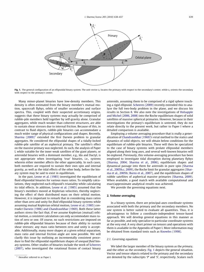
Fig. 1. The general configuration of an ellipsoidal binary system. The unit vector eP locates the primary with respect to the secondary’s center, while eS orients the secondarywith respect to the primary’s center.

I. Sharma / Icarus 205 (2010) 638–657 639

Many minor-planet binaries have low-density members. Thisdensity is often estimated from the binary member’s mutual mo-tion, spacecraft flybys, orbits of smaller secondaries and surfacespectra. This, coupled with their suspected accretionary origins,suggests that these binary systems may actually be comprised ofrubble-pile members held together by self-gravity alone. Granularaggregates, while much weaker than coherent structures, are ableto sustain shear stresses due to internal friction. Because of this, incontrast to fluid objects, rubble-pile binaries can accommodate amuch wider range of physical configurations and shapes. Recently,Sharma (2009)1 extended the first Darwin problem to granularaggregates. He considered the ellipsoidal shapes of a tidally-lockedrubble-pile satellite of an aspherical primary. The satellite’s effecton the massive primary was neglected. As such, the analysis of PaperI, while suitable for the inner weak satellites of the giant planets, orasteroidal binaries with a dominant member, e.g., Ida and Dactyl, isnot appropriate when investigating ‘true’ binaries, i.e., systemswherein either member affects the other appreciably. In such cases,both members are required to sustain their own spin and internalgravity, as well as the tidal effects of the other body, before the bin-ary system may be said to exist in equilibrium.

In the past, Leone et al. (1985) investigated the equilibrium offluid ellipsoidal binaries for various mass ratios. To simplify calcu-lations, they neglected each ellipsoid’s triaxiality while calculatingits tidal effects. In addition, Leone et al. (1985) assumed that thebinary’s members moved at Keplerian velocities, thereby neglect-ing the effect of their distributed mass on their orbital motion.However, it is important to remark that in considering mass ratiosother than zero and unity for fluid ellipsoidal binary systems whileassuming mutual Keplerian orbital motion, Leone et al. (1985) con-tradict Darwin (1906) and Chandrasekhar (1969). Both these latterauthors stress the fact that, if we assume Keplerian (mutual) orbi-tal motion, a consistent calculation can only accommodate mass ra-tios of zero or one. Of course, no such restrictions are imposed onrubble-pile ellipsoidal binaries because of their ability to sustainshear stresses; any mass ratio between zero and unity is accept-able. Additionally, many more shapes at a given orbital separation,mass ratio and internal friction angle are now possible. We willclarify this issue by outlining an incrementally consistent proce-dure to find the ellipsoidal equilibrium shapes of unequal fluid bin-ary systems. Other studies of binaries include the work of Scheeres(2007), who investigated the rotational fission of contact binary

1 Hereafter referred to as Paper I.

asteroids, assuming them to be comprised of a rigid sphere touch-ing a rigid ellipsoid. Scheeres (2009) recently extended this to ana-lyze the full two-body problem in the plane, and we discuss hisresults in Section 8. We also note the investigations of Holsappleand Michel (2006, 2008) into the Roche equilibrium shapes of solidsatellites of massive spherical primaries. However, because in theirinvestigations the primary’s equilibrium is untested, they do notrelate directly to the present work, but rather to Paper I where adetailed comparison is available.

Employing a volume-averaging procedure that is really a gener-alization of Chandrasekhar (1969)’s virial method to the statics anddynamics of solid objects, we will obtain below conditions for theequilibrium of rubble-pile binaries. These will then be specializedto the case of binary systems with prolate ellipsoidal membersaligned along their long axes, and several well-known binaries willbe explored. Previously, this volume-averaging procedure has beenemployed to investigate tidal disruption during planetary flybys(Sharma, 2004; Sharma et al., 2006), equilibrium shapes anddynamical passage into them for asteroids in pure spin (Sharmaet al., 2005b,c, 2009), the Roche limit for granular aggregates (Shar-ma et al., 2005b; Burns et al., 2007), and the equilibrium shapes ofrubble satellites of aspherical massive primaries (Sharma, 2009).When available, a good match with available computational andexact/approximate analytical results was achieved.

We provide the governing equations next.

2. Volume-averaging

In a binary system, there are principal-axes coordinate systemsassociated with both the primary and the secondary members. Noone system is better suited to evaluate all quantities. Thus, it isadvantageous to follow a coordinate-independent tensor-basedapproach. We will develop general equations in this manner asfar as possible, and only specialize to particular coordinate systemsat the very end. A very short primer on tensors and operations withthem is available in the Appendix of Paper I. More information maybe obtained from standard texts such as Knowles (1998).

2.1. Governing equations

We label the larger member of the binary system as the primary,and the other as the secondary. Fig. 1 depicts the general situation.Vector and tensor objects related to the primary and the secondaryare denoted by the subscripts ‘P’ and ‘S’, respectively. Scalars such

640 I. Sharma / Icarus 205 (2010) 638–657

as density, mass and volume are identified by primes – singleprimes ð0Þ refer to the primary and double primes ð00Þ to the sec-ondary. Stresses rP and rS within the binary’s members may be ob-tained by solving simultaneously the Navier equations

$P � rP þ q0bP ¼ q0ð€xP þ €RPÞ ð1aÞand $S � rS þ q00bS ¼ q00ð€xS þ €RSÞ; ð1bÞ

where the subscript ‘P’ (‘S’) on $ indicates differentiation with re-spect to xP ðxSÞ;q is a member’s density, b is the internal bodyforce,2 x is the location of a material point within a member with re-spect to its center of mass, and RP and RS locate the primary’s and thesecondary’s mass centers with respect to the binary system’s fixedcenter of mass; see Fig. 1. Note that €xP þ €RP ð€xS þ €RSÞ is the totalacceleration of a material point, and €xP ð€xSÞ is the acceleration rela-tive to the primary’s (secondary’s) mass centre. We make theassumption that the binary system rotates at a rate much faster thanits motion around the Sun. The body force within one of the binary’smembers includes, in our case, that object’s internal gravity and thetidal effects due to its companion. The effects of rotation enterthrough the inertial terms. For a complete definition of the problem,appropriate boundary conditions need to be specified for each mem-ber, and the relevant constitutive behavior of the primary and thesecondary have to be incorporated through compatibility equations;see, e.g., Fung (1965). Except in the simplest of geometries, loadingconditions, small deformations and linear rheologies, solving forthe exact stresses is often analytically intractable, and even compu-tationally very involved. Further, considering that little is knownabout the possibly intricate constitutive nature of planetary bodies,undertaking such an exercise may even be unjustified.

Here, we take an approximate route to estimate stresses withinthe binary’s members: volume-averaging. Volume-averaging relieson making a suitable low-order kinematic approximation to the ac-tual time-varying deformation of a body. Equations describing theevolution of the parameters governing this approximation are ob-tained by integrating over the body’s volume an appropriate ordermoment of the linear momentum balance Eqs. (1a) and (1b). Theprimary advantage of projecting the actual motion onto a low orderdeformation field is that we reduce the governing partial differen-tial equations to second-order ordinary differential equations. Inaddition, many different materials, physical configurations, anddynamical situations may be easily explored. Finally, volume-aver-aging is amenable to systematic improvements via a choice ofhigher-order kinematic approximations, see, e.g., Papadopoulos(2001).

In the present work, the motion of the binary’s members isapproximated by the simplest non-trivial deformation – the homo-geneous deformation – which prescribes that each ellipsoidal mem-ber may only deform into another, possibly rotated, stretched andsheared ellipsoid. This motion may be specified in terms of the ninecomponents of a time-dependent tensor FðtÞ, called the deforma-tion gradient tensor (see, e.g., Spencer, 1980), that relates the initial(X) and final (x) locations of a material point relative to an ellip-soid’s mass center. Thus, for the primary P and the secondary S,we write

xP ¼ FP � XP and xS ¼ FS � XS:

Alternatively, by defining the velocity gradient tensor

LðtÞ ¼ _FðtÞ � F�1ðtÞ; ð2Þwe specify the primary’s and the secondary’s motion in the incre-mental form

_xS ¼ LS � xS ð3aÞand _xP ¼ LP � xP: ð3bÞ

2 Note that because we have factored out the density, b has units of acceleration.

The governing equations may now be phrased in terms of L’scomponents.

We now follow the procedure, presented in several alternateways in Chandrasekhar (1969), Sharma et al. (2006, 2009) and Pa-per I, to relate the dynamics to the volume-averaged stress, i.e.,�r ¼

RV rdV within the binary’s members. We obtain the equations

ð _LP þ L2PÞ � IP ¼ MT

P � �rPV 0 ð4aÞand ð _LS þ L2

S Þ � IS ¼ MTS � �rSV 00; ð4bÞ

where V is a member’s volume,

I ¼Z

Vqx� xdV ð5Þ

is its inertia tensor,3 and

M ¼Z

Vx� qbdV ð6Þ

is the moment tensor due to the body forces b. Because the defor-mation and velocity gradient tensors are constant throughout thebody at any fixed time, so the stress, which typically depends onthese two tensors, is also independent of x. Thus, within the homo-geneous approximation, the average stress coincides with its actualvalue, and we henceforth drop the overbar on �r.

In a dynamic situation, the members’ shapes change, and so alsotheir inertia tensors. This evolution may be followed by first differ-entiating (5) while conserving mass, and then invoking (3b) and (5)to obtain

_IP ¼ LP � IP þ ðIP � LPÞT ð7aÞand _IS ¼ LS � IS þ ðIS � LSÞT : ð7bÞ

Equations (2), (4), and (7) govern the motion of the homogeneouslydeforming ellipsoids that comprise a binary system under the ac-tion of only the body forces b, once a constitutive law relating thestress r to a body’s deformation is specified.

Because we are presently interested in equilibrium shapes, thevelocity gradient L of the binary’s member collapses to a spin tensorW; the stretching rate component of L vanishes. The tensor Wmeasures the local angular velocity in a deformable medium, andis usually distinct from the rotation rate of a member’s principalaxes. However, at equilibrium, when the binary’s members rotatein a rigid manner, W coincides with the rotational angular velocity.Assuming that, at equilibrium, the binary’s members are tidally-locked and move on circular orbits about the binary system’s centerof mass, so that _W � 0, (4) simplifies and rearranges to

rP ¼1V 0

MTP �W2

P � IP

� �ð8aÞ

and rS ¼1

V 00MT

S �W2S � IS

� �: ð8bÞ

Each equation above expresses the average stress in a binary’smember in terms of the ‘centrifugal’ stresses due to rotation andstresses due to body forces as approximated by M. The above stressestimate, along with a suitable yield criterion, will help put con-straints on each member’s equilibrium shape for a given spin andseparation from its tidally-locked companion, as demonstrated be-low. We reemphasize that the above equations are valid for all bin-ary systems with ellipsoidal members that are mutually tidally-locked and on circular orbits about the common center of mass.To address binaries whose members are not tidally locked and/ormove on elliptic orbits (Marchis et al., 2007), we would have to re-tain _W in the above equations.

3 In indical notation, ðx� xÞij ¼ xixj .

I. Sharma / Icarus 205 (2010) 638–657 641

To estimate the average stress from (8), we need to evaluate thebody force moment tensor M. In our case, the body force in a bin-ary’s member is due both to its internal gravity, and also the tidalstresses introduced by its companion. Thus, we write

M ¼MG þMQ ; ð9Þ

where MG is the gravitational moment tensor because of internalgravity, and MQ , the quadrupole moment tensor, is the moment ten-sor due to tidal influence. Expressions for these tensors applicableto all mutually interacting triaxial ellipsoidal objects on possiblyelliptical orbits have been developed in Paper I, and here we providea only material essential to the present investigation. We refer thereader to Sections 2.3 and 2.4 of Paper I for more details.

2.2. Gravitational moment tensor

MG for ellipsoidal bodies may be expressed as

MG ¼ �2pqGI � A; ð10Þ

where G is the gravitational constant and the gravitational shapetensor A captures the effect of a body’s ellipsoidal shape on its inter-nal gravity (Chandrasekhar, 1969 or Sharma et al., 2006). The sym-metric tensor A depends only on the axes ratios a ¼ a2=a1 andb ¼ a3=a1, and is completely known for any given ellipsoid. Relevantformulae for A’s components are given in Section 2.4 of Sharmaet al. (2009). In particular, in its principal axes coordinate system,for a prolate ellipsoidal binary member,

A1 ¼ �2b2

1� b2 �b2

ð1� b2Þ3=2 ln1þ

ffiffiffiffiffiffiffiffiffiffiffiffiffiffi1� b2

qb

0@

1A

24

35 ð11aÞ

and A2 ¼ A3 ¼1

1� b2 �b2

ð1� b2Þ3=2 ln1þ

ffiffiffiffiffiffiffiffiffiffiffiffiffiffi1� b2

qb

0@

1A; ð11bÞ

where b ¼ a3=a1 is the axes ratio measuring the prolateness of thatmember.

2.3. Quadrupole moment tensor

Paper I develops MQ for two interacting triaxial ellipsoids. Theforce per unit mass due to an ellipsoid, say the binary system’s sec-ondary, of density qS and principal axes a00i at a point located exter-nally at XP with respect to the secondary’s center is given by

bQP ¼dFS

dm0¼ �2pq00GBS � XP;

where the symmetric tidal shape tensor BS depends only on the a00iand XP , and captures the effect of the ellipsoidal secondary’s asphe-ricity on its gravitational attraction. We will provide formulae forthe tidal shape tensor for a prolate ellipsoid in Section 4.1. Expres-sions for an oblate body are provided in Section 4.1 of Paper I.

The above formula for bQP is then employed in (6) to find thequadrupole moment MQP exerted by the binary’s secondary onits primary. When calculating MQP , the integration in (6) is overthe primary’s volume. Because BS’s components are complicatedfunctions, it is necessary to resort to a series expansion to obtaina useful expression for MQP . The tensor BS is expanded in a Taylorseries about the primary’s center of mass as

BS � Bð0ÞS þBð1ÞS �xP

Rþ Bð2ÞS :

xP � xP

R2 ; ð12Þ

where R is the separation of the binary’s members (see Fig. 1),XP ¼ xP þ R eP , and Bð1ÞS and B

ð2ÞS are third- and fourth-order tensors,

respectively. More information about these higher-order tensorsand operations with them may be found in the Appendix of Paper

I. For immediate use, we employ the summation convention to notethe formulae ða �AÞjk ¼ aiAijk; ðA � aÞij ¼ Aijkak; and ðA : a� bÞij ¼Aijklalbk for third- and fourth-order tensors A and A, respectively,and vectors a and b.

Utilizing expansion (12) results in the formula given by Eq. (23)of Paper I:

MQP ¼ �2pq00GIP � Bð0ÞS þ eP � Bð1ÞS

� �T� �

; ð13Þ

which is the quadrupole moment exerted by the secondary binarymember on the primary. Note that MQP depends on the tensorsBð0ÞS and Bð1ÞS that have subscript S. Similarly, the tidal effect on thesecondary due to the primary is

MQS ¼ �2pq0GIS � Bð0ÞP þ eS �Bð1ÞP

� �T� �

; ð14Þ

where, now, eS is a unit vector that locates the secondary with re-spect to the primary. Again, note that MQS depends on the tensorsBð0ÞP and Bð1ÞP with subscript P.

To utilize expressions (13) and (14) we need to develop formu-lae for the tensors Bð0Þ and Bð1Þ. As we will see in the next section,we also require Bð2Þ. Their calculation is complicated as there aremany possible relative orientations of the binary’s members. Thus,vector and tensor components depend on whether we view themin the primary’s (P) or the satellite’s (S) principal axes coordinatesystem. In keeping with Sharma’s (2009) notation, we will employð0Þ and ð00Þ to identify vector and tensor components in P and S,respectively. Note that BS, and so consequently, the various tensorsoccurring in its expansion (12), are diagonal when viewed in S.Similarly, BP and its concomitant tensors are diagonal in the pri-mary’s coordinate system P.

Paper I outlines a procedure to compute Bð0Þ;Bð1Þ and Bð2Þ, and inSection 4.1 provides Bð0Þ and Bð1Þ for an oblate object. Typically, wefirst calculate the B0iP – the components of BP in P – or B00iS – the compo-nents of BS in S – via available integral definitions; see Paper I, Eq. (18).From these, BP ’s components in S – the B00ijP – or BS’s components in P –

the B0ijS – are obtained by appealing to the rotation tensor that relatesthe secondary’s and primary’s coordinate systems S and P, respec-tively. For this we require the tensor coordinate transformation for-mulae available in the Appendix of Paper I. Employing the B0ijS and

the B00ijP , we compute the second-, third- and fourth-order tidal shapetensors in the expansions of BP and BS. Here we will do so for binarieswith prolate ellipsoidal members aligned along their long axes.

2.4. Orbital motion

The gravitational attraction between two triaxial ellipsoids wasobtained in Paper I. Employing that formula, an expression was de-rived for the angular velocity of one ellipsoid on a circular orbitabout another. Applying Eq. (25) of Paper I to the binary’s primary,we find its angular velocity

x02 ¼ 2pq00GeP � Bð0ÞS � eP þ1

m0R2 Bð1ÞS þ eP � Bð2ÞS

� �: IP

� �m00 þm0

m00;

ð15Þ

correct to Oða03i =R3Þ. Note the absence of the first-order terms ða0i=RÞ.Similarly, the secondary’s angular velocity is

x002 ¼ 2pq0GeS � Bð0ÞP � eS þ1

m00R2 Bð1ÞP þ eS � Bð2ÞP

� �: IS

� �m00 þm0

m0:

ð16Þ

We again refer the reader to the Appendix of Paper I for informationon tensor operations employed above. Here, we simply note that forvector a, and second-, third- and fourth-order tensors B;A and A,

642 I. Sharma / Icarus 205 (2010) 638–657

respectively, the computations ðA : BÞi ¼ AijkBkj and a � ðA : BÞj ¼aiAijklBlk result in vectors. Thus, the terms within the square bracketsabove are, in fact, vectors. In the above formulae for x0, the firstterm is what would result if we assumed that the primary’s entiremass were located at its center. The next two terms bring in the ef-fect of the primary’s distributed mass on its orbital motion. A sim-ilar interpretation holds for x00.

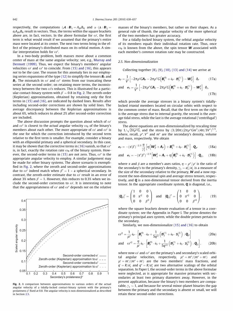
In a two-body problem, both masses move about a commoncenter of mass at the same angular velocity; see, e.g., Murray andDermott (1999). Thus, we expect the binary’s members’ angularvelocities x0 and x00 to coincide. From (15) and (16), this appearsnot to be the case. The reason for this anomaly lies in our employ-ing series expansions of the type (12) to simplify the tensors BP andBS. The mismatch in x0 and x00 stems from our truncating theseseries at the second order; on retaining more terms, the inconsis-tency between the two x’s reduces. This is illustrated for a partic-ular contact-binary system with b0 ¼ 0:8 in Fig. 2. The zeroth-order(Keplerian) approximations, obtained by retaining only the firstterms in (15) and (16), are indicated by dashed lines. Results afterincluding second-order corrections are shown by solid lines. Theaverage discrepancy between the Keplerian approximations isabout 6%, which reduces to about 2% after second-order correctionare included.

The above discussion prompts the question about which of x0

and x00 is closest to the actual angular velocity xB of the binary’smembers about each other. The more appropriate of x0 and x00 isthe one for which the correction introduced by the second termrelative to the first term is smaller. For example, consider a binarywith an ellipsoidal primary and a spherical secondary. In this case,it may be shown that the corrective terms in (16) vanish, so that x00

is, in fact, exactly the rotation rate xB of the binary system. How-ever, the second-order terms in (15) are not zero. Thus, x00 is theappropriate angular velocity to employ. A similar judgement maybe made for other binary systems. The above scenario is exempli-fied in Fig. 2, where the zeroth and second-order approximationsdue to x00 indeed match when b00 ¼ 1 – a spherical secondary. Incontrast, the zeroth-order estimate due to x0 result in an error ofabout 3% when b0 ¼ 1. However, this reduces to 0.3% when we in-clude the second-order correction to x0. It is interesting to notethat the appropriateness of x0 and x00 depends not on the relative

0.1 0.2 0.3 0.4 0.5 0.6 0.7 0.8 0.9 10.05

0.1

0.15

0.2

0.25

0.3

0.35

0.4

Zeroth-order (Keplerian) approximation to ω

Zeroth-order (Keplerian) approximation to ω

Second-order corrected ω

Second-order corrected ω

Scal

ed a

ngul

ar v

eloc

ity

Secondary’s prolateness β

Fig. 2. A comparison between approximations to various orders of the actualangular velocity of a tidally-locked contact-binary system with the primary’sprolateness b0 fixed at 0.8. The angular velocity is non-dimensionalized as describedin Section 2.5.

masses of the binary’s members, but rather on their shapes. As ageneral rule of thumb, the angular velocity of the more sphericalof the two members has greater accuracy.

For a tidally-locked binary system, the orbital angular velocityof its members equals their individual rotation rate. Thus, oncexB is known from the above, the spin tensor W associated witheach member’s common rotation rate may be constructed.

2.5. Non-dimensionalization

Collecting together (8), (9), (10), (13) and (14) we arrive at

rP ¼1V 0�2pq0GAP � 2pq00G Bð0ÞS þ eP �Bð1ÞS

� ��W2

P

h i� IP ð17aÞ

and rS ¼1

V 00�2pq00GAS � 2pq0G Bð0ÞP þ eS �Bð1ÞP

� ��W2

S

h i� IS;

ð17bÞ

which provide the average stresses in a binary system’s tidally-locked triaxial members located on circular orbits with respect tothe common center of mass. Recall, that the first term on the rightis the average stress due to internal gravity, the second is the aver-age tidal stress, while the last is the average rotational (‘centrifugal’)stress.

The above equations are non-dimensionalized by rescaling timeby 1=

ffiffiffiffiffiffiffiffiffiffiffiffiffiffiffi2pq00G

p, and the stress by ð3=20pÞð2pq00Gm00Þð4p=3V 00Þ1=3,

where, recall, q00;V 00 and m00 are the secondary’s density, volumeand mass, respectively. We obtain

rP ¼ �ða0b0Þ�2=3 gc2

1

g W2P þ AP

� �þ Bð0ÞS þ eP � Bð1ÞS

h i� Q P ð18aÞ

and rS ¼ �ða00b00Þ�2=3 W2S þ AS þ g Bð0ÞP þ eS � Bð1ÞP

� �h i� Q S; ð18bÞ

where a and b are a member’s axes ratios, g ¼ q00=q0 is the ratio ofthe secondary’s to the primary’s density, c1 ¼ a001=a01 is a measure ofthe size of the secondary relative to the primary, W and r now rep-resent the non-dimensional spin and average stress tensors, respec-tively, and Q is a non-dimensional tensor derived from the inertiatensor. In the appropriate coordinate system, Q is diagonal, i.e.,

½Q P�0 ¼

1 0 00 a02 00 0 b02

0B@

1CA and ½Q S�

00 ¼1 0 00 a002 00 0 b002

0B@

1CA; ð19Þ

where the square brackets denote evaluation of a tensor in a coor-dinate system; see the Appendix in Paper I. The prime denotes theprimary’s principal axes system, while the double primes pertain tothe secondary.

Similarly, we non-dimensionalize (15) and (16) to obtain

x02 ¼ 1l00

eP � Bð0ÞS � eP þ1

5q02Bð1ÞS þ eP � Bð2ÞS

� �: Q P

� �ð20aÞ

and x002 ¼ gl0

eS � Bð0ÞP � eS þ1

5q002Bð1ÞP þ eS � Bð2ÞP

� �: Q S

� �; ð20bÞ

where now x0 and x00 are the primary’s and secondary’s scaled orbi-tal angular velocities, respectively, l00 ¼ m00=ðm00 þm0Þ andl0 ¼ m0=ðm00 þm0Þ are the two members’ mass fractions, andq0 ¼ R=a01 and q00 ¼ R=a001 are two alternative scalings of the orbitalseparation. In Paper I, the second-order terms in the above formulaewere neglected, as is appropriate for massive primaries with sec-ondaries at least two primary diameters away. However, in thepresent application, because the binary’s two members are compa-rable, c1 � 1, and because for several minor-planet binaries the gapbetween the primary and the secondary is absent or small, we willretain these second-order corrections.

I. Sharma / Icarus 205 (2010) 638–657 643

2.6. Coordinate systems

We are concerned with a tidally-locked binary system, so thatthe spins of the two objects are equal and match their orbital rota-tion rate about the common center of mass. For a tidally-lockedconfiguration to be tenable, the principal axes of the primary andthe secondary must be parallel, though not necessarily in an or-dered manner, i.e., e0i need not be parallel to e00i . We will, however,assume the ellipsoidal members’ shortest axes, along e03 and e003,respectively, are normal to the orbital plane. This choice isprompted by the predictions of Burns and Safronov (1973) andSharma et al. (2005a) that dissipative objects tend to align into astate of pure rotation about their axes of maximum inertia. Theremaining two axes for each binary member will be set as needed.

We will evaluate (18a) in P, and (18b) in S. The forms of the ten-sors Q P and Q S in P and S, respectively, are given above in (19). Thegravitational shape tensor A is diagonal in its parent coordinatesystem, i.e.,

½AP �0 ¼A01P

0 0

0 A03P0

0 0 A03P

0BB@

1CCA and ½AS�00 ¼

A001S0 0

0 A003S0

0 0 A003S

0BB@

1CCA;

ð21Þ

with A1 and A3 for prolate ellipsoids given by (11). The non-dimen-sional spin tensors become

½WP�0 ¼ ½WS�00 ¼0 �W3 0

W3 0 00 0 0

0B@

1CA ð22Þ

where, because the binary’s members are tidally locked,

W3 ¼ xB; ð23Þ

the common orbital rotation rate of the two bodies about the bin-ary’s mass center. Recall from Section 2.4 that xB is taken to bex0 or x00 depending on the relative accuracy of formulae (15) and(16).

The tidal shape tensors BP and BS and their accompanying ten-sors Bð0ÞP ;Bð0ÞS , etc., will be found first in their parent coordinate sys-tem, and then transformed to the principal axes system of itsneighbor when required. This transformation depends on the rela-tive orientation of the members’ coordinate systems, i.e., P and S.They will be derived for the example configuration in Section 4. Fi-nally, the primary’s stress-tensor components in P, and the second-ary’s in S, will be taken to be r0ijP and r00ijS , respectively.

The exact volume-averaged stresses in a tidally-locked, triaxial-ellipsoidal members of a binary as they move on circular orbitsabout a common center of mass are given by (18). However, thesestresses cannot take arbitrary values for rubble piles that yield un-der high-enough shear stresses. The next section introduces a yieldcriterion for such granular aggregates that will help put bounds onthe possible shapes, densities and mutual separations that rubble-pile binaries may achieve before one or both of its membersdisrupt.

3. Rheology

An appropriate rheology for cohesionless granular aggregates isdiscussed in Section 3 of Paper I. There these materials are modeledas rigid-perfectly plastic materials obeying the Drucker–Prageryield criterion; see, e.g., Chen and Han (1988). Thus the aggregateresponds in a rigid manner unless the average stress violates theDrucker–Prager condition. Much more information about model-ing rubble piles as rigid-perfectly plastic materials is provided inSharma (2004) or Sharma et al. (2009).

Granular aggregates have finite resistance to shear (Nedderman,1992), due both to the usual interfacial friction because of particleinteraction, as well as a geometric friction resulting from interlock-ing of finite-sized members. Because of its frictional roots, theshear resistance of rubble piles depends on internal pressure. TheDrucker–Prager rule is a pressure-dependent yield criterion thatattempts to capture this finite shear strength of granular aggre-gates. To formulate the Drucker–Prager yield criterion, we definethe pressure

p ¼ �13

tr r; ð24Þ

where ‘tr’ denotes a tensor’s trace, and the deviatoric stress tensor

s ¼ rþ p1: ð25Þ

The Drucker–Prager yield condition may then be written as

jsj2 6 k2p2; ð26Þ

where, applying the summation convention,

jsj ¼ffiffiffiffiffiffiffiffiffisijsij

pis the magnitude of the deviatoric stress, and

k ¼ 2ffiffiffi6p

sin /F

3� sin /Fð27Þ

depends on the internal friction angle /F . As the friction angle liesbetween 0� and 90;0 6 k 6

ffiffiffi6p

. Finally, in terms of the three prin-cipal stresses ri, the definition above for jsjmay be put into the illu-minating form

jsj2 ¼ 13½ðr2 � r3Þ2 þ ðr3 � r1Þ2 þ ðr1 � r2Þ2� ¼

23

s21 þ s2

2 þ s23

� �;

ð28Þ

where si ¼ jrj � rkj=2; ði – j – kÞ are the principal shear stresses ata point, so that jsjmay be thought of as a measure of the ‘total’ localshear stress. Thus, the Drucker–Prager yield criterion (26), alongwith (27), puts a limit on the allowable local shear stresses in termsof the local pressure and the internal friction angle. This interpreta-tion will be found useful later to understand yielding in tidally-locked members of binary systems.

4. Example: Prolate binary system

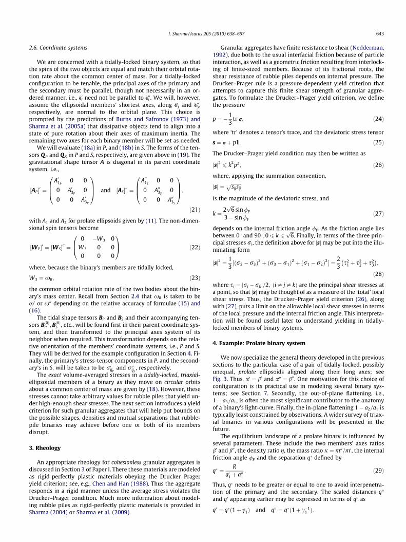
We now specialize the general theory developed in the previoussections to the particular case of a pair of tidally-locked, possiblyunequal, prolate ellipsoids aligned along their long axes; seeFig. 3. Thus, a0 ¼ b0 and a00 ¼ b00. One motivation for this choice ofconfiguration is its practical use in modeling several binary sys-tems; see Section 7. Secondly, the out-of-plane flattening, i.e.,1� a3=a1, is often the most significant contributor to the anatomyof a binary’s light-curve. Finally, the in-plane flattening 1� a2=a1 istypically least constrained by observations. A wider survey of triax-ial binaries in various configurations will be presented in thefuture.

The equilibrium landscape of a prolate binary is influenced byseveral parameters. These include the two members’ axes ratiosb0 and b00, the density ratio g, the mass ratio j ¼ m00=m0, the internalfriction angle /F and the separation q defined by

q ¼ Ra01 þ a001

: ð29Þ

Thus, q needs to be greater or equal to one to avoid interpenetra-tion of the primary and the secondary. The scaled distances q00

and q0 appearing earlier may be expressed in terms of q as

q0 ¼ qð1þ c1Þ and q00 ¼ qð1þ c�11 Þ:

Fig. 3. A binary with prolate members aligned along their long axes. The axes e0i of P and e00i of S coincide. The orbital plane is normal to e03. The unit vector eP (eS) locates theprimary (secondary) with respect to the secondary’s (primary’s) center.

644 I. Sharma / Icarus 205 (2010) 638–657

The size ratio c1 introduced in Section 2.5 is related to other param-eters by

c1 ¼jg

b02

b002

!1=3

:

We will assume that the density ratio g is one. This choice is moti-vated by the common suspicion that binaries are consequences ofpast disruption events. This is also why we employ the same inter-nal friction angle for both the primary and the secondary. We willprobe the five-dimensional ðb00 � b0 � q � /F � jÞ equilibrium land-scape graphically by taking appropriate two-dimensional sections.More concretely, for several combinations of q;/F and j, we willfind regions in b00 � b0 space that delineate where a binary systemmay exist.

The average stresses within the tidally-locked prolate primaryand secondary on circular orbits about a common center of massare evaluated in their local principal coordinate systems by settinga0 ¼ b0 and a00 ¼ b00 in (18) along with (19) and (11). The spin ten-sors are substituted from (22) and (23) after following Section 2.4’sprescription for obtaining the binary’s rotation rate xB. We willalso require expressions for the tensors Bð0Þ;Bð1Þ and Bð2Þ associatedwith each member in its companion’s principal coordinate system,

e.g., Bð0ÞP in S: Bð0ÞP

h i0. These tensors will be obtained below. We will

hence obtain the average stresses in the primary and the second-ary, i.e., rP and rS, respectively. Employing these stresses withthe yield criterion (26), will help generate bounds that delineatethe equilibrium landscape of each member of the binary systemas a function of its shape, its companion’s shape, their mutual sep-aration, and their internal composition as modeled by /F . Recallthat in a tidally-locked configuration, the binary’s separation islinked to its members’ spin via (23). From the individual boundsof the primary and the secondary, composite bounds for the binarysystem will be recovered.

In Fig. 3, two prolate ellipsoids with a01 P a02 ¼ a03 anda001 P a002 ¼ a003 are located a distance R apart. These two objects arealigned along their long axes, so that e01 and e001 are parallel. Boththe primary’s and the secondary’s third axes are taken to be normalto the orbital plane. With these choices, Fig. 3 shows that e0i and e00iare the same, and the rotation tensor T relating P and S is simply anidentity tensor, i.e.,

T ¼ 1: ð30ÞWe also see that eS ¼ �eP ¼ e001. We now obtain the various tidalshape tensors and their expansions in appropriate coordinatesystems.

4.1. Bð0Þ;Bð1Þ and Bð2Þ

As mentioned earlier, we ultimately require Bð0ÞP

h i00; Bð1ÞP

h i00and

Bð2ÞP

h i00, and Bð0ÞS

h i0; Bð1ÞS

h i0and B

ð2ÞS

h i0. The former are the components

in S of the tensors in the primary’s tidal shape tensor BP ’s expan-sion, while the latter are the components in P of tensors in BS’sseries; see (12). To obtain these matrices, we will follow Section 4of Paper I. In addition, we will outline the procedure only for quan-tities associated with the secondary. An identical process will yieldthe matrices in S of tensors in BP ’s approximation.

The components B00iS – the components of BS in S – for a prolatesecondary, i.e., a001 P a002 ¼ a003, are found via the integral formulae inSection 2.3 of Paper I:

B001S¼ � 2

p0022

ffiffiffiffiffiffiffiffiffiffiffiffiffiffiffiffiffia0023 þ k00

q � 1

p003=22

ln

ffiffiffiffiffiffiffiffiffiffiffiffiffiffiffiffiffia0021 þ k00

q� p0022ffiffiffiffiffiffiffiffiffiffiffiffiffiffiffiffiffi

a0021 þ k00q

þ p0022

ð31aÞ

and

B002S¼ B003S

¼

ffiffiffiffiffiffiffiffiffiffiffiffiffiffiffiffiffia0021 þ k00

qp0022 ða0023 þ k00Þ þ

1

2p003=22

ln

ffiffiffiffiffiffiffiffiffiffiffiffiffiffiffiffiffia0021 þ k00

q� p0022ffiffiffiffiffiffiffiffiffiffiffiffiffiffiffiffiffi

a0021 þ k00q

þ p0022

; ð31bÞ

where p002 ¼ffiffiffiffiffiffiffiffiffiffiffiffiffiffiffiffiffiffiffia0021 � a0023

q, and the ellipsoidal coordinate k00 is the

greatest solution of the equation

X0021P

a0021 þ k00þ

X0022P

a0022 þ k00þ

X 0023P

a0023 þ k00¼ 1; ð32Þ

where we recall that XP ¼ xP þ ReP is the location of a material pointin the primary with respect to the secondary’s center, and X00iP areXP ’s components in S. Note that upon dividing by a0031 we may ex-press (31b) in terms of a scaled orbital radius q00 ¼ R=a001, and the sec-ondary’s axes ratio b00 ¼ a003=a001. Employing (30) with the tensorcoordinate transformation formulae found in the Appendix of PaperI, we obtain

B0ijS ¼ B00iS dij ðno sumÞ; ð33Þ

i.e., because P and S are identical, so too are BS’s components in thetwo frames. Similarly, for the vector XP ; x00iP ¼ x0iP

Now, following Section 4.1 of Paper I, a series solution to (32) fork00 in powers of x00iP=R is generated. This is then substituted into the

formulae for B0ijS obtained from (33) and (31). The resulting expres-

sion is expanded up to Oðx002iP=R2Þ to find an expression similar to BS’s

expansion (12). This yields the components of the tensors Bð0ÞS ;Bð1ÞS

and Bð2ÞS in P, the primary’s coordinate system. In particular, after

non-dimensionalizing as suggested in the previous paragraph,

B0ð0Þ11S¼ � 2b002

q00ð1� b002Þ� b002

ð1� b002Þ3=2 lnq00 �

ffiffiffiffiffiffiffiffiffiffiffiffiffiffiffiffi1� b002

qq00 þ

ffiffiffiffiffiffiffiffiffiffiffiffiffiffiffiffi1� b002

q

ð34aÞ

and

B0ð0Þ22S¼ B0ð0Þ33S

¼ b002q00

q002o ð1� b002Þþ b002

2ð1� b002Þ3=2 lnq00 �

ffiffiffiffiffiffiffiffiffiffiffiffiffiffiffiffi1� b002

qq00 þ

ffiffiffiffiffiffiffiffiffiffiffiffiffiffiffiffi1� b002

q

; ð34bÞ

10o

20o

30o

10o

1o

1o

Secondary with φF=1o

survives

Primary with φF = 1o

survives

3o

5o

0.9

0.1

0.2

0.3

0.4

0.5

0.6

0.7

0.8

1

0.90.1 0.2 0.3 0.4 0.5 0.6 0.7 0.8 1

Primary’s prolateness, ’ = a3’/a1’β

Seco

ndar

y’s

prol

aten

ess,

’ =

a 3’/a

1’β

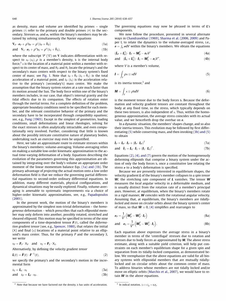
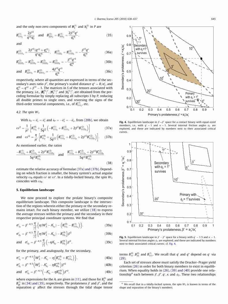
Fig. 4. Equilibrium landscape in b0—b00 space for a contact binary with equal-sizedmembers, i.e., with q ¼ 1 and j ¼ 1. Several internal friction angles /F areexplored, and these are indicated by numbers next to their associated criticalcurves.

0.1 0.2 0.3 0.4 0.5 0.6 0.7 0.8 0.9 1

0.9

0.1

0.2

0.3

0.4

0.5

0.6

0.7

0.8

1

Primary’s prolateness, β’ = a3’/a1’

Seco

ndar

y’s

prol

aten

ess,

β’’ =

a3’’

/a1’’

3o

5o

10o

20o

30o

1o

Secondarywith φF = 1o

survives

Primary withφF = 1osurvives

Fig. 5. Equilibrium landscape in b0 � b00 space for a binary with q ¼ 1:5 and j ¼ 1.Several internal friction angles /F are explored, and these are indicated by numbersnext to their associated critical curves; cf. Fig. 4.

4 We recall that in a tidally-locked system, the spin W3 is known in terms of theshape and separation of the binary’s members.

I. Sharma / Icarus 205 (2010) 638–657 645

and the only non-zero components of Bð1ÞS and Bð2ÞS in P are

B0ð1Þ111S¼ 2b002

q002q00oand B0ð1Þ221S

¼ B0ð1Þ331S¼ 2b002q00

q004o; ð35Þ

and

B0ð2Þ1111S¼ 2b002ðq002 þ q002o Þ

q00q004o; B0ð2Þ1122S

¼ B0ð2Þ1133S¼ � b002q00

q004oð36aÞ

B0ð2Þ2222S¼ B0ð2Þ2233S

¼ B0ð2Þ3322S¼ B0ð2Þ3333S

¼ � b002q003

q006oð36bÞ

and B0ð2Þ2211S¼ B0ð2Þ3311S

¼ �4b002q003

q006o; ð36cÞ

respectively, where all quantities are expressed in terms of the sec-ondary’s axes ratio b00, the primary’s scaled distance q00 ¼ R=a001, andq002o ¼ q002 þ b002 � 1. The matrices in S of the tensors associated withthe primary, i.e., ½Bð0ÞP �

00; ½Bð1ÞP �

00 and ½Bð2ÞP �00, are obtained from the pre-

ceding formulae by simply replacing all subscripts S by P, reducingall double primes to single ones, and reversing the signs of thethird-order tensorial components, i.e., of B0ð1Þ111S

, etc.

4.2. The spin W3

With eS ¼ e01 ¼ e001 and eP ¼ �e001 ¼ �e01, from (20b), we obtain

x02 ¼ 1l00

B0ð0Þ11Sþ 1

5q02�B0ð1Þ111S

þ B0ð2Þ1111Sþ 2b02B0ð2Þ1133S

� �� �ð37aÞ

and x002 ¼ gl0

B00ð0Þ11Pþ 1

5q002B00ð1Þ111P

þ B00ð2Þ1111Pþ 2b002B00ð2Þ1133P

� �� �: ð37bÞ

As mentioned earlier, the ratios

�B0ð1Þ111Sþ B0ð2Þ1111S

þ 2b02B0ð2Þ1133S

5q02B0ð0Þ11S

andB00ð1Þ111P

þ B00ð2Þ1111Pþ 2b002B00ð2Þ1133P

5q002B00ð0Þ11P

ð38Þ

estimate the relative accuracy of formulae (37a) and (37b). Depend-ing on which fraction is smaller, the binary system’s actual angularvelocity xB equals x0 or x00. In a tidally-locked binary, the spin W3

coincides with xB.

5. Equilibrium landscape

We now proceed to explore the prolate binary’s compositeequilibrium landscape. This composite landscape is the intersec-tion of the regions wherein either the primary or the secondary re-mains intact. For each binary member, we utilize (18) to expressthe average stresses within the primary and the secondary in theirrespective principal coordinate systems. We find that

r01P¼ b0�4=3 g

c21

gðW23 � A01P

Þ � B0ð0Þ11S� B0ð1Þ111S

� �n o; ð39aÞ

r02P¼ b0�4=3 g

c21

gðW23 � A03P

Þ � B0ð0Þ33S

n ob02 ð39bÞ

and r03P¼ b0�4=3 g

c21

�gA03P� B0ð0Þ33S

� �b02; ð39cÞ

for the primary, and analogously, for the secondary,

r001S¼ b00�4=3 W2

3 � A001S� g B00ð0Þ11P

þ B00ð1Þ111P

� �n o; ð40aÞ

r002S¼ b00�4=3 W2

3 � A003S� gB00ð0Þ33P

� �b002 ð40bÞ

and r003S¼ b00�4=3 �A003S

� gB00ð0Þ33P

� �b002; ð40cÞ

where expressions for the Ai are given in (11), and those for Bð0Þij andBð1Þijk in (34) and (35), respectively. The prolateness b0 and b00, and theseparation q affect the stresses through the tidal shape tensor

terms Bð0Þ11 ;Bð0Þ33 and Bð1Þ111. We recall that q0 and q00 depend on q via

(29).Each set of stresses above must satisfy the Drucker–Prager yield

criterion (26) in order for both binary members to exist in equilib-rium. When equality holds in (26), (39) and (40) provide one rela-tionship4 each between b0; b00; q;j and /F . These two relationships

3o5o

10o

20o

30o

1o

Secondarysurvives

Primarysurvives

20o

Secondarysurvives

3o

5o

10o

20o

30o

1o

Secondarysurvives

Primarysurvives

5o

1o

20o

30o

40o

90o30o

40 o

0.9

0.1

0.2

0.3

0.4

0.5

0.6

0.7

0.8

1

0.9

0.1

0.2

0.3

0.4

0.5

0.6

0.7

0.8

1

0.9

0.1

0.2

0.3

0.4

0.5

0.6

0.7

0.8

1

0.90.1 0.2 0.3 0.4 0.5 0.6 0.7 0.8 1Primary’s prolateness, ’ = a3’/a1’

3o

5o

10o

20o

30o

10o

β

Seco

ndar

y’s

prol

aten

ess,

’ =

a 3’/a

1’β

Seco

ndar

y’s

prol

aten

ess,

’ =

a 3’/a

1’β

Seco

ndar

y’s

prol

aten

ess,

’ =

a 3’/a

1’β

0.90.1 0.2 0.3 0.4 0.5 0.6 0.7 0.8 1Primary’s prolateness, ’ = a3’/a1’β

1o 1o

20o

30o

1o

10o

3o

5o

1o

1o

3o

3o

20o

20o

Primarysurvives

Secondarysurvives

Primarysurvives

3o

5o

10o

20o

30o

1o

Secondarysurvives

1o

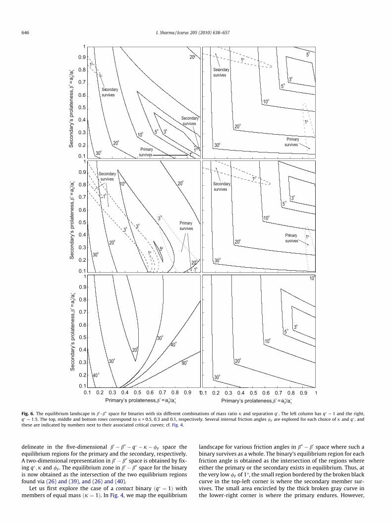
Fig. 6. The equilibrium landscape in b0–b00 space for binaries with six different combinations of mass ratio j and separation q . The left column has q ¼ 1 and the right,q ¼ 1:5. The top, middle and bottom rows correspond to j = 0.5, 0.3 and 0.1, respectively. Several internal friction angles /F are explored for each choice of j and q , andthese are indicated by numbers next to their associated critical curves; cf. Fig. 4.

646 I. Sharma / Icarus 205 (2010) 638–657

delineate in the five-dimensional b0 � b00 � q � j� /F space theequilibrium regions for the primary and the secondary, respectively.A two-dimensional representation in b0 � b00 space is obtained by fix-ing q;j and /F . The equilibrium zone in b0 � b00 space for the binaryis now obtained as the intersection of the two equilibrium regionsfound via (26) and (39), and (26) and (40).

Let us first explore the case of a contact binary ðq ¼ 1Þ withmembers of equal mass ðj ¼ 1Þ. In Fig. 4, we map the equilibrium

landscape for various friction angles in b00 � b0 space where such abinary survives as a whole. The binary’s equilibrium region for eachfriction angle is obtained as the intersection of the regions whereeither the primary or the secondary exists in equilibrium. Thus, atthe very low /F of 1�, the small region bordered by the broken blackcurve in the top-left corner is where the secondary member sur-vives. The small area encircled by the thick broken gray curve inthe lower-right corner is where the primary endures. However,

1

1.1

1.3

1.51.8

2

1

1.1

1.51.8

1.3

2

Secondary survives above this curve

Primary survives to the right of this curve

0.9

0.1

0.2

0.3

0.4

0.5

0.6

0.7

0.8

1

0.90.1 0.2 0.3 0.4 0.5 0.6 0.7 0.8 1Primary’s prolateness, ’ = a3’/a1’β

Seco

ndar

y’s

prol

aten

ess,

’ =

a 3’/a

1’β

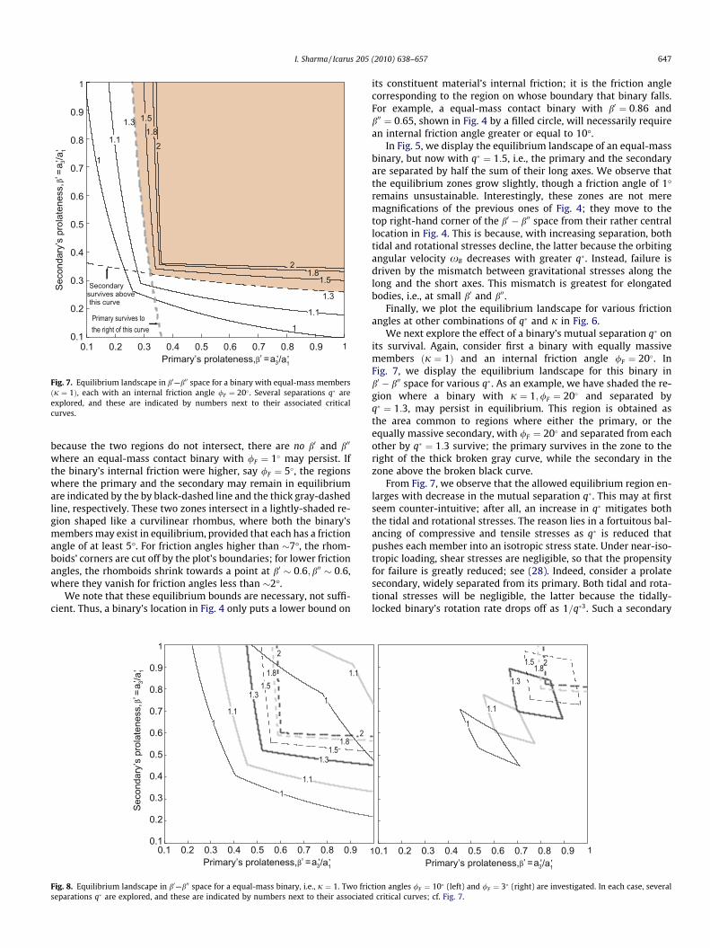
Fig. 7. Equilibrium landscape in b0—b00 space for a binary with equal-mass membersðj ¼ 1Þ, each with an internal friction angle /F ¼ 20 . Several separations q areexplored, and these are indicated by numbers next to their associated criticalcurves.

I. Sharma / Icarus 205 (2010) 638–657 647

because the two regions do not intersect, there are no b0 and b00

where an equal-mass contact binary with /F ¼ 1 may persist. Ifthe binary’s internal friction were higher, say /F ¼ 5, the regionswhere the primary and the secondary may remain in equilibriumare indicated by the by black-dashed line and the thick gray-dashedline, respectively. These two zones intersect in a lightly-shaded re-gion shaped like a curvilinear rhombus, where both the binary’smembers may exist in equilibrium, provided that each has a frictionangle of at least 5�. For friction angles higher than �7�, the rhom-boids’ corners are cut off by the plot’s boundaries; for lower frictionangles, the rhomboids shrink towards a point at b0 � 0:6; b00 � 0:6,where they vanish for friction angles less than �2�.

We note that these equilibrium bounds are necessary, not suffi-cient. Thus, a binary’s location in Fig. 4 only puts a lower bound on

1

11.1

1.1

1.3

1.31.5

1.8

2

1.1

1

1.81.5

2

0.9

0.1

0.2

0.3

0.4

0.5

0.6

0.7

0.8

0.90.1 0.2 0.3 0.4 0.5 0.6 0.7 0.8

1

Primary’s prolateness, ’ = a3’/a1’β

Seco

ndar

y’s

prol

aten

ess,

’ =

a 3’/a

1’β

Fig. 8. Equilibrium landscape in b0—b00 space for a equal-mass binary, i.e., j ¼ 1. Two fricseparations q are explored, and these are indicated by numbers next to their associate

its constituent material’s internal friction; it is the friction anglecorresponding to the region on whose boundary that binary falls.For example, a equal-mass contact binary with b0 ¼ 0:86 andb00 ¼ 0:65, shown in Fig. 4 by a filled circle, will necessarily requirean internal friction angle greater or equal to 10�.

In Fig. 5, we display the equilibrium landscape of an equal-massbinary, but now with q ¼ 1:5, i.e., the primary and the secondaryare separated by half the sum of their long axes. We observe thatthe equilibrium zones grow slightly, though a friction angle of 1�remains unsustainable. Interestingly, these zones are not meremagnifications of the previous ones of Fig. 4; they move to thetop right-hand corner of the b0 � b00 space from their rather centrallocation in Fig. 4. This is because, with increasing separation, bothtidal and rotational stresses decline, the latter because the orbitingangular velocity xB decreases with greater q. Instead, failure isdriven by the mismatch between gravitational stresses along thelong and the short axes. This mismatch is greatest for elongatedbodies, i.e., at small b0 and b00.

Finally, we plot the equilibrium landscape for various frictionangles at other combinations of q and j in Fig. 6.

We next explore the effect of a binary’s mutual separation q onits survival. Again, consider first a binary with equally massivemembers ðj ¼ 1Þ and an internal friction angle /F ¼ 20. InFig. 7, we display the equilibrium landscape for this binary inb0 � b00 space for various q. As an example, we have shaded the re-gion where a binary with j ¼ 1;/F ¼ 20 and separated byq ¼ 1:3, may persist in equilibrium. This region is obtained asthe area common to regions where either the primary, or theequally massive secondary, with /F ¼ 20 and separated from eachother by q ¼ 1:3 survive; the primary survives in the zone to theright of the thick broken gray curve, while the secondary in thezone above the broken black curve.

From Fig. 7, we observe that the allowed equilibrium region en-larges with decrease in the mutual separation q. This may at firstseem counter-intuitive; after all, an increase in q mitigates boththe tidal and rotational stresses. The reason lies in a fortuitous bal-ancing of compressive and tensile stresses as q is reduced thatpushes each member into an isotropic stress state. Under near-iso-tropic loading, shear stresses are negligible, so that the propensityfor failure is greatly reduced; see (28). Indeed, consider a prolatesecondary, widely separated from its primary. Both tidal and rota-tional stresses will be negligible, the latter because the tidally-locked binary’s rotation rate drops off as 1=q3. Such a secondary

1

1.1

1.3

1.51.8

2

1 0.90.1 0.2 0.3 0.4 0.5 0.6 0.7 0.8 1Primary’s prolateness, ’ = a3’/a1’β

tion angles /F ¼ 10 (left) and /F ¼ 3 (right) are investigated. In each case, severald critical curves; cf. Fig. 7.

648 I. Sharma / Icarus 205 (2010) 638–657

will fail only due to shear stress developed as a result of the mis-match between the large gravitational compressive stress alongthe long axis e001, and the smaller one along any one of the two shortaxes. As this object is brought closer to the primary, mutual inter-action introduces tensile stresses along the principal axes. How-ever, the tensile stress along the e001 is far greater, because boththe rotational and tidal stresses are much more significant in thisdirection; see Fig. 3. In contrast, rotational stresses are smalleralong the short-axis e002, and non-existent along e003. Similarly, tidal

11.1

1.31.5 2

1.81

11.1

1.31.5

21.8

1.3

1.8

1.1

1

1.1

1

1.51.8

2

1.5

1.82

1.51.3

1.82

1.8

1.1

1

0.9

0.1

0.2

0.3

0.4

0.5

0.6

0.7

0.8

1

0.90.1 0.2 0.3 0.4 0.5 0.6 0.7 0.8Primary’s prolateness, ’ = a3’/a1’β

Seco

ndar

y’s

prol

aten

ess,

’ =

a 3’/a

1’β

0.9

0.1

0.2

0.3

0.4

0.5

0.6

0.7

0.8

1

Seco

ndar

y’s

prol

aten

ess,

’ =

a 3’/a

1’β

0.9

0.1

0.2

0.3

0.4

0.5

0.6

0.7

0.8

1

Seco

ndar

y’s

prol

aten

ess,

’ =

a 3’/a

1’β

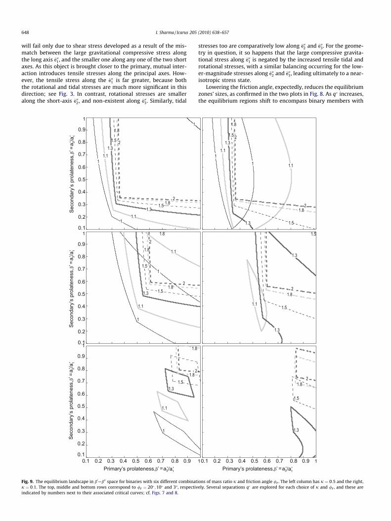
Fig. 9. The equilibrium landscape in b0—b00 space for binaries with six different combinatj ¼ 0:1. The top, middle and bottom rows correspond to /F ¼ 20 ;10 and 3�, respectivindicated by numbers next to their associated critical curves; cf. Figs. 7 and 8.

stresses too are comparatively low along e002 and e003. For the geome-try in question, it so happens that the large compressive gravita-tional stress along e001 is negated by the increased tensile tidal androtational stresses, with a similar balancing occurring for the low-er-magnitude stresses along e002 and e003, leading ultimately to a near-isotropic stress state.

Lowering the friction angle, expectedly, reduces the equilibriumzones’ sizes, as confirmed in the two plots in Fig. 8. As q increases,the equilibrium regions shift to encompass binary members with

1 1.1

21.8

1.5

11.1

1.31.5

1.8

2

1.3

1.5

1.11.5

1.3

1.82

1.3

1.5

1.3

1.82

1 0.90.1 0.2 0.3 0.4 0.5 0.6 0.7 0.8 1Primary’s prolateness, ’ = a3’/a1’β

ions of mass ratio j and friction angle /F . The left column has j ¼ 0:5 and the right,ely. Several separations q are explored for each choice of j and /F , and these are

0.8

0.5 0.8 1

0.5

0.1

0.3

0.3

0.3

0.5

0.1

1

0.9

0.1

0.2

0.3

0.4

0.5

0.6

0.7

0.8

1

0.90.1 0.2 0.3 0.4 0.5 0.6 0.7 0.8 1Primary’s prolateness, ’ = a3’/a1’β

Seco

ndar

y’s

prol

aten

ess,

’ =

a 3’/a

1’β

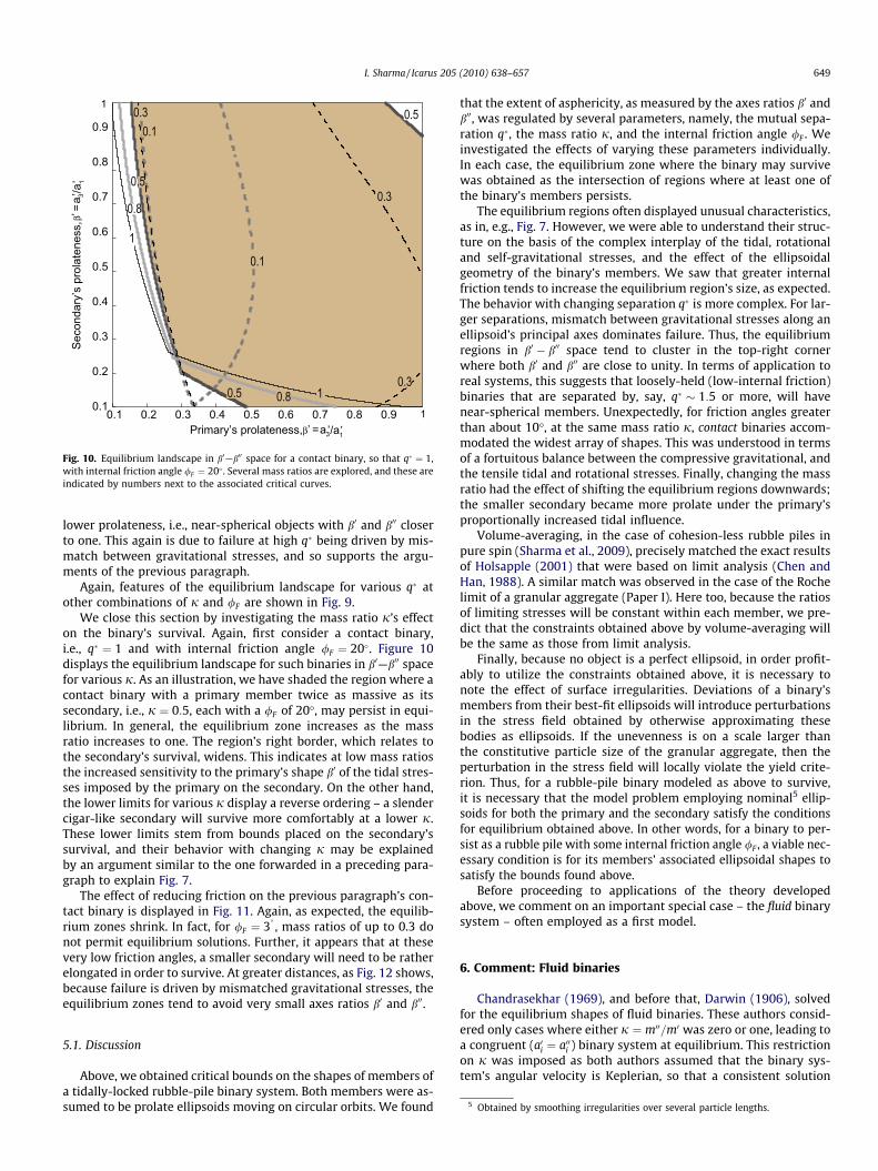
Fig. 10. Equilibrium landscape in b0—b00 space for a contact binary, so that q ¼ 1,with internal friction angle /F ¼ 20 . Several mass ratios are explored, and these areindicated by numbers next to the associated critical curves.

I. Sharma / Icarus 205 (2010) 638–657 649

lower prolateness, i.e., near-spherical objects with b0 and b00 closerto one. This again is due to failure at high q being driven by mis-match between gravitational stresses, and so supports the argu-ments of the previous paragraph.

Again, features of the equilibrium landscape for various q atother combinations of j and /F are shown in Fig. 9.

We close this section by investigating the mass ratio j’s effecton the binary’s survival. Again, first consider a contact binary,i.e., q ¼ 1 and with internal friction angle /F ¼ 20. Figure 10displays the equilibrium landscape for such binaries in b0—b00 spacefor various j. As an illustration, we have shaded the region where acontact binary with a primary member twice as massive as itssecondary, i.e., j ¼ 0:5, each with a /F of 20�, may persist in equi-librium. In general, the equilibrium zone increases as the massratio increases to one. The region’s right border, which relates tothe secondary’s survival, widens. This indicates at low mass ratiosthe increased sensitivity to the primary’s shape b0 of the tidal stres-ses imposed by the primary on the secondary. On the other hand,the lower limits for various j display a reverse ordering – a slendercigar-like secondary will survive more comfortably at a lower j.These lower limits stem from bounds placed on the secondary’ssurvival, and their behavior with changing j may be explainedby an argument similar to the one forwarded in a preceding para-graph to explain Fig. 7.

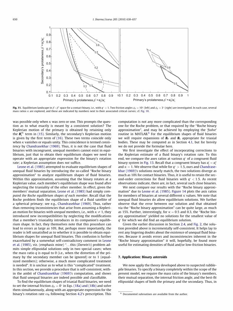
The effect of reducing friction on the previous paragraph’s con-tact binary is displayed in Fig. 11. Again, as expected, the equilib-rium zones shrink. In fact, for /F ¼ 3

, mass ratios of up to 0.3 do

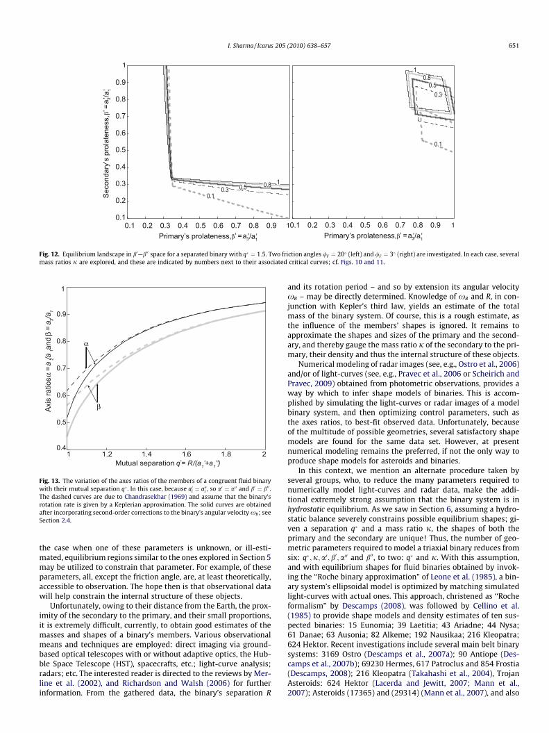
not permit equilibrium solutions. Further, it appears that at thesevery low friction angles, a smaller secondary will need to be ratherelongated in order to survive. At greater distances, as Fig. 12 shows,because failure is driven by mismatched gravitational stresses, theequilibrium zones tend to avoid very small axes ratios b0 and b00.

5 Obtained by smoothing irregularities over several particle lengths.

5.1. Discussion

Above, we obtained critical bounds on the shapes of members ofa tidally-locked rubble-pile binary system. Both members were as-sumed to be prolate ellipsoids moving on circular orbits. We found

that the extent of asphericity, as measured by the axes ratios b0 andb00, was regulated by several parameters, namely, the mutual sepa-ration q, the mass ratio j, and the internal friction angle /F . Weinvestigated the effects of varying these parameters individually.In each case, the equilibrium zone where the binary may survivewas obtained as the intersection of regions where at least one ofthe binary’s members persists.

The equilibrium regions often displayed unusual characteristics,as in, e.g., Fig. 7. However, we were able to understand their struc-ture on the basis of the complex interplay of the tidal, rotationaland self-gravitational stresses, and the effect of the ellipsoidalgeometry of the binary’s members. We saw that greater internalfriction tends to increase the equilibrium region’s size, as expected.The behavior with changing separation q is more complex. For lar-ger separations, mismatch between gravitational stresses along anellipsoid’s principal axes dominates failure. Thus, the equilibriumregions in b0 � b00 space tend to cluster in the top-right cornerwhere both b0 and b00 are close to unity. In terms of application toreal systems, this suggests that loosely-held (low-internal friction)binaries that are separated by, say, q � 1:5 or more, will havenear-spherical members. Unexpectedly, for friction angles greaterthan about 10�, at the same mass ratio j, contact binaries accom-modated the widest array of shapes. This was understood in termsof a fortuitous balance between the compressive gravitational, andthe tensile tidal and rotational stresses. Finally, changing the massratio had the effect of shifting the equilibrium regions downwards;the smaller secondary became more prolate under the primary’sproportionally increased tidal influence.

Volume-averaging, in the case of cohesion-less rubble piles inpure spin (Sharma et al., 2009), precisely matched the exact resultsof Holsapple (2001) that were based on limit analysis (Chen andHan, 1988). A similar match was observed in the case of the Rochelimit of a granular aggregate (Paper I). Here too, because the ratiosof limiting stresses will be constant within each member, we pre-dict that the constraints obtained above by volume-averaging willbe the same as those from limit analysis.

Finally, because no object is a perfect ellipsoid, in order profit-ably to utilize the constraints obtained above, it is necessary tonote the effect of surface irregularities. Deviations of a binary’smembers from their best-fit ellipsoids will introduce perturbationsin the stress field obtained by otherwise approximating thesebodies as ellipsoids. If the unevenness is on a scale larger thanthe constitutive particle size of the granular aggregate, then theperturbation in the stress field will locally violate the yield crite-rion. Thus, for a rubble-pile binary modeled as above to survive,it is necessary that the model problem employing nominal5 ellip-soids for both the primary and the secondary satisfy the conditionsfor equilibrium obtained above. In other words, for a binary to per-sist as a rubble pile with some internal friction angle /F , a viable nec-essary condition is for its members’ associated ellipsoidal shapes tosatisfy the bounds found above.

Before proceeding to applications of the theory developedabove, we comment on an important special case – the fluid binarysystem – often employed as a first model.

6. Comment: Fluid binaries

Chandrasekhar (1969), and before that, Darwin (1906), solvedfor the equilibrium shapes of fluid binaries. These authors consid-ered only cases where either j ¼ m00=m0 was zero or one, leading toa congruent (a0i ¼ a00i ) binary system at equilibrium. This restrictionon j was imposed as both authors assumed that the binary sys-tem’s angular velocity is Keplerian, so that a consistent solution

0.8

0.3

0.51

0.5

0.81

0.30.5

0.8

1

0.9

0.1

0.2

0.3

0.4

0.5

0.6

0.7

0.8

0.90.1 0.2 0.3 0.4 0.5 0.6 0.7 0.8 1

1

Primary’s prolateness, ’ = a3’/a1’β

0.90.1 0.2 0.3 0.4 0.5 0.6 0.7 0.8 1Primary’s prolateness, ’ = a3’/a1’β

Seco

ndar

y’s

prol

aten

ess,

’ =

a 3’/a

1’β

Fig. 11. Equilibrium landscape in b0—b00 space for a contact binary, i.e., with q ¼ 1. Two friction angles /F ¼ 10 (left) and /F ¼ 3 (right) are investigated. In each case, severalmass ratios j are explored, and these are indicated by numbers next to their associated critical curves; cf. Fig. 10.

6 Documented subroutines are available from the author.

650 I. Sharma / Icarus 205 (2010) 638–657

was possible only when j was zero or one. This prompts the ques-tion as to what exactly is meant by a consistent solution? TheKeplerian motion of the primary is obtained by retaining onlythe Bð0ÞS term in (15). Similarly, the secondary’s Keplerian motionis given by the first term of (16). These two terms coincide onlywhen j vanishes or equals unity. This coincidence is termed consis-tency by Chandrasekhar (1969). Thus, it is not the case that fluidbinaries with incongruent, unequal members cannot exist in equi-librium, just that to obtain their equilibrium shapes we need tooperate with an appropriate expression for the binary’s rotationrate; a Keplerian assumption does not suffice.

Leone et al. (1985) attempted to evaluate equilibrium shapes ofunequal fluid binaries by introducing the so-called ‘‘Roche binaryapproximation” to analyze equilibrium shapes of fluid binaries.Within this approximation, assuming that the binary rotates at aKeplerian value, each member’s equilibrium shape was found afterneglecting the triaxiality of the other member. In effect, given themembers’ mutual separation, Leone et al. (1985) had simply com-puted the Roche equilibrium shapes of each member. Recall that theRoche problem finds the equilibrium shape of a fluid satellite ofa spherical primary; see e.g., Chandrasekhar (1969). Thus, ratherthan removing inconsistencies that arise from assuming a Kepleri-an motion for binaries with unequal members, i.e., with j – 1, theyintroduced new incompatibilities by neglecting the modificationsthat a member’s triaxiality introduces in its companion’s equilib-rium shape. In fact, they themselves note that this procedure canlead to errors as large as 10%. But, perhaps more importantly, thereader is left unsatisfied as to whether it is possible to obtain equi-librium shapes for unequal fluid binaries. This confusion is furtherexacerbated by a somewhat self-contradictory comment in Leoneet al. (1985), viz. (emphasis mine) ‘‘. . .this (Darwin’s) problem ad-mits simple ellipsoidal solutions only in two special cases; whenthe mass ratio q is equal to 0 (i.e., when the distortion of the pri-mary by the secondary member can be ignored) or to 1 (equal-sized members); otherwise, a much more complicated treatmentis needed”. It is unclear as to what is this ‘‘complicated” treatment.In this section, we provide a procedure that is self-consistent, with-in the ambit of Chandrasekhar (1969)’s computation, and showsthat fluid unequal binaries are indeed possible and classifiable.

To find the equilibrium shapes of triaxial fluid binaries, we needto set the internal friction /F ¼ 0 in Eqs. (18a) and (18b) and solvethem simultaneously, along with an appropriate expression for thebinary’s rotation rate xB following Section 4.2’s prescription. This

computation is not any more complicated than the correspondingone for the Roche problem, or that required by the ‘‘Roche binaryapproximation”, and may be achieved by employing the ‘fsolve’routine in MATLAB.6 For the equilibrium shapes of fluid binarieswe will require expansions of BP and BS appropriate for triaxialbodies. These may be computed as in Section 4.1, but for brevitywe do not provide the formulae here.

We first investigate the effect of incorporating corrections tothe Keplerian estimate of a fluid binary’s rotation rate. To thisend, we compare the axes ratios at various q of a congruent fluidbinary system in Fig. 13. Recall that a congruent binary has a0i ¼ a00iand j ¼ 1. We observe that while for q > 1:5, ours and Chandrase-khar (1969)’s solutions nearly match, the two solutions diverge asmuch as 10% for contact binaries. Thus, it is useful to retain the sec-ond-order corrections for fluid binaries with q < 1:5. As recentobservations indicate, there are, in fact, several such close binaries.

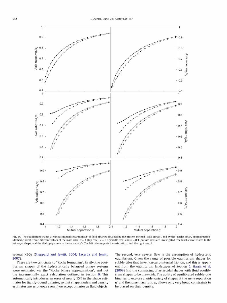
We next compare our results with the ‘‘Roche binary approxi-mation” due to Leone et al. (1985). Figure 14 plots the axis ratiosfor members of binaries at several different j values. We note thatunequal fluid binaries do allow equilibrium solutions. We furtherobserve that the error between our solution and that obtainedvia the ‘‘Roche binary approximation” can be quite large, as muchas 15%. Further, interestingly, for j ¼ 0:5 and 0.3, the ‘‘Roche bin-ary approximation” yielded no solutions for the smallest value ofq for which we did find an equilibrium solution.

Given the earlier discussion in Section 2.4, and Fig. 2, the solu-tion provided above is incrementally self-consistent. It helps lay torest any lingering doubts about the existence of unequal fluid bina-ries. Because it avoids errors and inconsistencies inherent in the‘‘Roche binary approximation” it will, hopefully, be found moreuseful for estimating densities of fluid and/or low-friction binaries.

7. Application: Binary asteroids

We now apply the theory developed above to suspected rubble-pile binaries. To specify a binary completely within the scope of thepresent model, we require the mass ratio of the binary’s members,their mutual separation, the internal friction angle, and the best-fitellipsoidal shapes of both the primary and the secondary. Thus, in

0.1

0.30.5

1

0.1

0.8

0.3 0.5 0.8 1

0.9

0.1

0.2

0.3

0.4

0.5

0.6

0.7

0.8

0.90.1 0.2 0.3 0.4 0.5 0.6 0.7 0.8 1

1

Primary’s prolateness, ’ = a3’/a1’β

0.90.1 0.2 0.3 0.4 0.5 0.6 0.7 0.8 1Primary’s prolateness, ’ = a3’/a1’β

Seco

ndar

y’s

prol

aten

ess,

’ =

a 3’/a

1’β

Fig. 12. Equilibrium landscape in b0—b00 space for a separated binary with q ¼ 1:5. Two friction angles /F ¼ 20 (left) and /F ¼ 3 (right) are investigated. In each case, severalmass ratios j are explored, and these are indicated by numbers next to their associated critical curves; cf. Figs. 10 and 11.

1 1.2 1.4 1.6 1.8 20.4

0.5

0.6

0.7

0.8

0.9

1

Axis

ratio

s α =

a2 /a

1 and

β =

a 3 /a1

Mutual separation q* = R/(a1’+a1’’)

α

β

Fig. 13. The variation of the axes ratios of the members of a congruent fluid binarywith their mutual separation q . In this case, because a0i ¼ a00i , so a0 ¼ a00 and b0 ¼ b00 .The dashed curves are due to Chandrasekhar (1969) and assume that the binary’srotation rate is given by a Keplerian approximation. The solid curves are obtainedafter incorporating second-order corrections to the binary’s angular velocity xB; seeSection 2.4.

I. Sharma / Icarus 205 (2010) 638–657 651

the case when one of these parameters is unknown, or ill-esti-mated, equilibrium regions similar to the ones explored in Section 5may be utilized to constrain that parameter. For example, of theseparameters, all, except the friction angle, are, at least theoretically,accessible to observation. The hope then is that observational datawill help constrain the internal structure of these objects.

Unfortunately, owing to their distance from the Earth, the prox-imity of the secondary to the primary, and their small proportions,it is extremely difficult, currently, to obtain good estimates of themasses and shapes of a binary’s members. Various observationalmeans and techniques are employed: direct imaging via ground-based optical telescopes with or without adaptive optics, the Hub-ble Space Telescope (HST), spacecrafts, etc.; light-curve analysis;radars; etc. The interested reader is directed to the reviews by Mer-line et al. (2002), and Richardson and Walsh (2006) for furtherinformation. From the gathered data, the binary’s separation R

and its rotation period – and so by extension its angular velocityxB – may be directly determined. Knowledge of xB and R, in con-junction with Kepler’s third law, yields an estimate of the totalmass of the binary system. Of course, this is a rough estimate, asthe influence of the members’ shapes is ignored. It remains toapproximate the shapes and sizes of the primary and the second-ary, and thereby gauge the mass ratio j of the secondary to the pri-mary, their density and thus the internal structure of these objects.

Numerical modeling of radar images (see, e.g., Ostro et al., 2006)and/or of light-curves (see, e.g., Pravec et al., 2006 or Scheirich andPravec, 2009) obtained from photometric observations, provides away by which to infer shape models of binaries. This is accom-plished by simulating the light-curves or radar images of a modelbinary system, and then optimizing control parameters, such asthe axes ratios, to best-fit observed data. Unfortunately, becauseof the multitude of possible geometries, several satisfactory shapemodels are found for the same data set. However, at presentnumerical modeling remains the preferred, if not the only way toproduce shape models for asteroids and binaries.

In this context, we mention an alternate procedure taken byseveral groups, who, to reduce the many parameters required tonumerically model light-curves and radar data, make the addi-tional extremely strong assumption that the binary system is inhydrostatic equilibrium. As we saw in Section 6, assuming a hydro-static balance severely constrains possible equilibrium shapes; gi-ven a separation q and a mass ratio j, the shapes of both theprimary and the secondary are unique! Thus, the number of geo-metric parameters required to model a triaxial binary reduces fromsix: q;j;a0; b0;a00 and b00, to two: q and j. With this assumption,and with equilibrium shapes for fluid binaries obtained by invok-ing the ‘‘Roche binary approximation” of Leone et al. (1985), a bin-ary system’s ellipsoidal model is optimized by matching simulatedlight-curves with actual ones. This approach, christened as ‘‘Rocheformalism” by Descamps (2008), was followed by Cellino et al.(1985) to provide shape models and density estimates of ten sus-pected binaries: 15 Eunomia; 39 Laetitia; 43 Ariadne; 44 Nysa;61 Danae; 63 Ausonia; 82 Alkeme; 192 Nausikaa; 216 Kleopatra;624 Hektor. Recent investigations include several main belt binarysystems: 3169 Ostro (Descamps et al., 2007a); 90 Antiope (Des-camps et al., 2007b); 69230 Hermes, 617 Patroclus and 854 Frostia(Descamps, 2008); 216 Kleopatra (Takahashi et al., 2004), TrojanAsteroids: 624 Hektor (Lacerda and Jewitt, 2007; Mann et al.,2007); Asteroids (17365) and (29314) (Mann et al., 2007), and also

0.4

0.5

0.6

0.7

0.8

0.9

1

Axis

ratio

α = a

2 /a1

0.4

0.5

0.6

0.7

0.8

0.9

1

Axis

ratio

α = a

2 /a1

0.4

0.5

0.6

0.7

0.8

0.9

1

Axis

ratio

α = a

2 /a1

0.4

0.5

0.6

0.7

0.8

0.9

1

Axis ratio α = a2 /a

1

0.4

0.5

0.6

0.7

0.8

0.9

1

Axis ratio α = a2 /a

1

0.4

0.5

0.6

0.7

0.8

0.9

1

Axis ratio α = a2 /a

1

1 1.2 1.4 1.6 1.8 2Mutual separation q*

1 1.2 1.4 1.6 1.8 2Mutual separation q*

Fig. 14. The equilibrium shapes at various mutual separations q of fluid binaries obtained by the present method (solid curves), and by the ‘‘Roche binary approximation”(dashed curves). Three different values of the mass ratio, j ¼ 1 (top row), j ¼ 0:5 (middle row) and j ¼ 0:3 (bottom row) are investigated. The black curve relates to theprimary’s shape, and the thick gray curve to the secondary’s. The left column plots the axis ratio a, and the right one, b.

652 I. Sharma / Icarus 205 (2010) 638–657

several KBOs (Sheppard and Jewitt, 2004; Lacerda and Jewitt,2007).

There are two criticisms to ‘‘Roche formalism”. Firstly, the equi-librium shapes of the hydrostatically balanced binary systemswere estimated via the ‘‘Roche binary approximation”, and notthe incrementally exact calculation outlined in Section 6. Thisautomatically introduces an error of nearly 15% in the shape esti-mates for tightly-bound binaries, so that shape models and densityestimates are erroneous even if we accept binaries as fluid objects.

The second, very severe, flaw is the assumption of hydrostaticequilibrium. Given the range of possible equilibrium shapes forrubble piles that have non-zero internal friction, and this is appar-ent from the equilibrium landscapes of Section 5, Harris et al.(2009) find the comparing of asteroidal shapes with fluid equilib-rium shapes to be untenable. The ability of equilibrated rubble-pilebinaries to explore a wide variety of shapes at the same separationq and the same mass ratio j, allows only very broad constraints tobe placed on their density.

3o5o

10o

20o

30o

10o

216 Kleopatra

0.9

0.1

0.2

0.3

0.4

0.5

0.6

0.7

0.8

1

0.90.1 0.2 0.3 0.4 0.5 0.6 0.7 0.8 1Primary’s prolateness, ’ = a3’/a1’β

Seco

ndar

y’s

prol

aten

ess,

’ =

a 3’/a

1’β

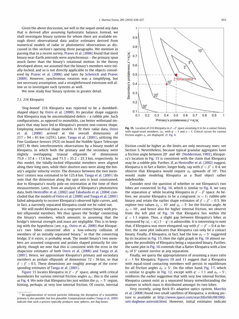
Fig. 15. Location of 216 Kleopatra in b0—b00 space assuming it to be a contact binarywith equal-sized members, i.e., with q ¼ 1 and j ¼ 1. Critical curves for variousfriction angles /F are displayed; cf. Fig. 4.

I. Sharma / Icarus 205 (2010) 638–657 653

Given the above discussion, we will in the sequel avoid any datathat is derived after assuming hydrostatic balance. Instead, weshall investigate binary systems for whom there are available en-ough direct observational data and/or estimates derived fromnumerical models of radar or photometric observations as dis-cussed in this section’s opening three paragraphs. We mention inpassing that in a recent survey, Pravec et al. (2006) found that mostbinary near-Earth asteroids were asynchronous – the primary spunmuch faster than the binary’s rotational motion. In the theorydeveloped above, we assumed that the binary’s members were tid-ally-locked, and so is not directly applicable to the objects consid-ered by Pravec et al. (2006) and later by Scheirich and Pravec(2009). However, synchronous rotation was a simplifying, butnot necessary assumption, and a straightforward extension will al-low us to investigate such systems as well.

We now study four binary systems in greater detail.

7.1. 216 Kleopatra

‘Dog-boned’ 216 Kleopatra was reported to be a dumbbell-shaped object by Ostro et al. (2000). Its peculiar shape suggeststhat Kleopatra may be unconsolidated debris – a rubble pile. Suchconfigurations, as opposed to monoliths, can better withstand im-pacts that may have led to Kleopatra’s present non-convex shape.Employing numerical shape models to fit their radar data, Ostroet al. (2000) arrived at the overall dimensions of217 � 94 � 81 km (±25%). Later, Tanga et al. (2001), utilizing theFine Guidance Sensors (FGS) on board the Hubble Space Telescope(HST) fit their interferometric observations by a binary model ofKleopatra, in which both the primary and the secondary wereslightly overlapping triaxial ellipsoids of dimensions75.9 � 37.4 � 17.6 km, and 71:5� 35:2� 25:3 km, respectively. Inthis model, the tidally-locked ellipsoidal members were alignedalong their long axes, while their shortest axes were along the bin-ary’s angular velocity vector. The distance between the two mem-bers’ centers was estimated to be 125.4 km. Tanga et al. (2001) donote that the dimension along the spin axis is least constrained,due to Kleopatra’s nearly pole-on orientation at the time of theirmeasurements. Later, from an analysis of Kleopatra’s photometricdata, both Hestroffer et al. (2002) and Takahashi et al. (2004) con-cluded that the models of Ostro et al. (2000) and Tanga et al. (2001)failed adequately to recover Kleopatra’s observed light-curves, and,in fact, a narrowly separated Kleopatra could not be ruled out.

We will model Kleopatra as a congruent contact binary with pro-late ellipsoidal members. We thus ignore the ‘bridge’ connectingthe binary’s members, which amounts to assuming that thebridge’s internal strength and mass are negligible. This is in keep-ing with the hypothesis (see, e.g., Ostro et al., 2000) that Kleopat-ra’s two lobes connected after a low-velocity collision ofmembers of an initially separated binary,7 so that the connectingbridge, if it exists, is probably weak. The model binary’s two mem-bers are assumed congruent and prolate shaped primarily for sim-plicity, though we note that this is consistent with the error in theshape/size estimates of both Ostro et al. (2000) and Tanga et al.(2001). Hence, we approximate Kleopatra’s primary and secondarymembers as prolate ellipsoids of dimensions 72 � 36 km, so thatb0 ¼ b00 ¼ 0:5. These dimensions are roughly average of the corre-sponding estimates of Tanga et al. (2001).

Figure 15 locates Kleopatra in b0 � b00 space, along with criticalboundaries for various internal friction angles /F; this is the sameas Fig. 4. We note that Kleopatra lies just within the /F ¼ 5 region,hinting, perhaps, at very low internal friction. Of course, internal

7 Re-agglomeration of several particles following the disruption of a monolithicprimary is also possible, but less plausible. Computational studies (Tanga et al., 2009indicate that such a process typically produces near spheres, not dog-bones.

)

friction could be higher as the limits are only necessary ones; seeSection 5. Nevertheless, because typical granular aggregates havea friction angle between 20 and 40 (Nedderman, 1992), Kleopat-ra’s location in Fig. 15 is consistent with the claim that Kleopatramay be a rubble pile. Further, if, as Hestroffer et al. (2002) suggest,Kleopatra is in fact a flatter, longer body, say with b0 ¼ b00 6 0:4, weobserve that Kleopatra would require /F upwards of 10�. Thiswould make modeling Kleopatra as a fluid object ratherindefensible.

Consider next the question of whether or not Kleopatra’s twolobes are connected. In Fig. 16, which is similar to Fig. 8, we varythe separation q while locating Kleopatra in b0 � b00 space. As be-fore, we assume Kleopatra to be a congruent ðj ¼ 1Þ rubble-pilebinary and retain the earlier shape estimates of b0 ¼ b00 ¼ 0:5. Weexplore two values /F ¼ 10 and /F ¼ 5 for the friction angle. At/F ¼ 10, and hence also for higher internal friction, we observefrom the left plot of Fig. 16 that Kleopatra lies within theq ¼ 1:1 region. Thus, a slight gap between Kleopatra’s lobes asmeasured by ða01 þ a001Þð1� qÞ is admissible. It is interesting to notethat, if Kleopatra was more elongated, say with b0 ¼ b00 ¼ 0:4 as be-fore, the same plot indicates that Kleopatra can only be a contactbinary. Finally, if Kleopatra, in fact, had the low /F ¼ 5 suggestedby its location in Fig. 15, then the right graph in Fig. 16 almost ne-gates the possibility of Kleopatra being a separated binary. Further,the same plot in Fig. 16 contends that a flatter Kleopatra with a low/F of 5� cannot survive at any separation.

Finally, we query the appropriateness of assuming a mass ratioj ¼ 1 for Kleopatra. Figures 10 and 11 suggest that a Kleopatrawith equal-sized contacting members will persist in equilibriumfor all friction angles /F P 5. On the other hand, Fig. 17, whichis similar to graphs in Fig. 12, except with q ¼ 1:1 and /F ¼ 5,reinforces the earlier suggestion that with very low internal friction,Kleopatra cannot exist as a separated binary notwithstanding themanner in which mass is distributed amongst its two lobes.

Very recently, using Keck II’s adaptive optics system, Marchiset al. (2008) found two small satellites of Kleopatra; a striking pic-ture is available at http://www.space.com/searchforlife/081002-seti-dogbone-asteroid.html. However, initial estimates indicate

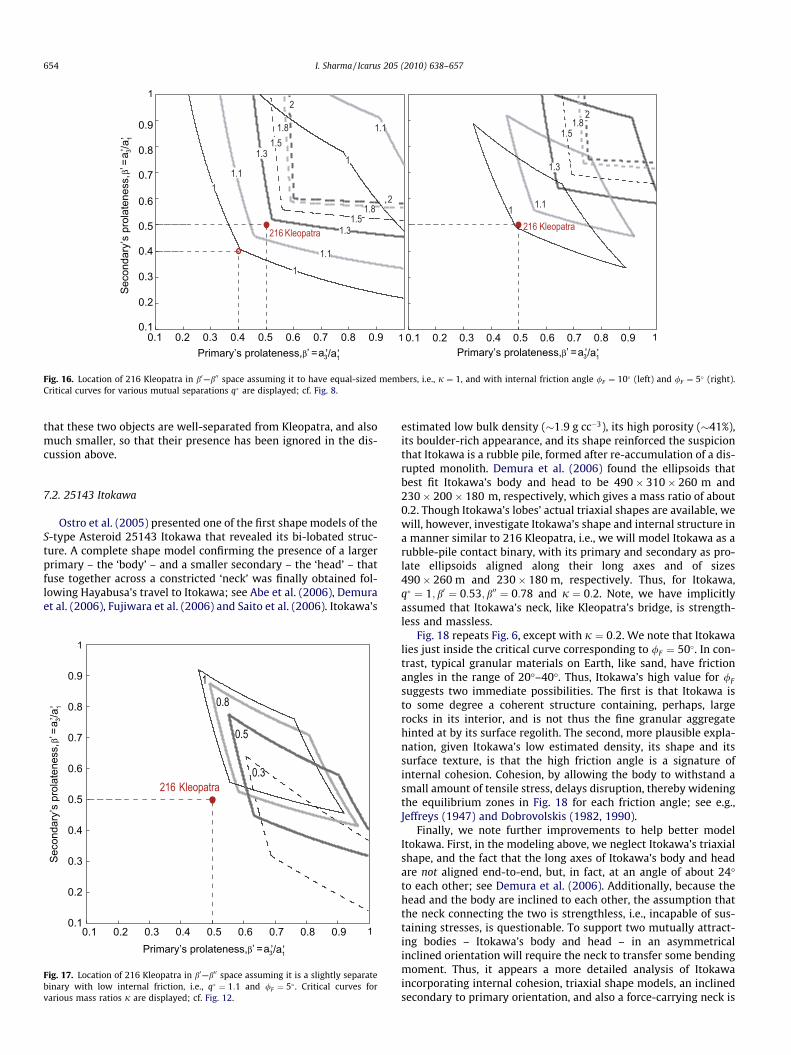
1

11.1

1.1

1.3

1.31.5

1.8

2

1.1

1

1.81.5

2

216 Kleopatra 216 Kleopatra1 1.1

1.51.8

2

1.3

0.9

0.1

0.2

0.3

0.4

0.5

0.6

0.7

0.8

1

0.90.1 0.2 0.3 0.4 0.5 0.6 0.7 0.8 1Primary’s prolateness, ’ = a3’/a1’β

0.90.1 0.2 0.3 0.4 0.5 0.6 0.7 0.8 1Primary’s prolateness, ’ = a3’/a1’β

Seco

ndar

y’s

prol

aten

ess,

’ =

a 3’/a

1’β

Fig. 16. Location of 216 Kleopatra in b0—b00 space assuming it to have equal-sized members, i.e., j ¼ 1, and with internal friction angle /F ¼ 10 (left) and /F ¼ 5 (right).Critical curves for various mutual separations q are displayed; cf. Fig. 8.

654 I. Sharma / Icarus 205 (2010) 638–657

that these two objects are well-separated from Kleopatra, and alsomuch smaller, so that their presence has been ignored in the dis-cussion above.

7.2. 25143 Itokawa

Ostro et al. (2005) presented one of the first shape models of theS-type Asteroid 25143 Itokawa that revealed its bi-lobated struc-ture. A complete shape model confirming the presence of a largerprimary – the ‘body’ – and a smaller secondary – the ‘head’ – thatfuse together across a constricted ‘neck’ was finally obtained fol-lowing Hayabusa’s travel to Itokawa; see Abe et al. (2006), Demuraet al. (2006), Fujiwara et al. (2006) and Saito et al. (2006). Itokawa’s

216 Kleopatra

0.8

0.5

1

0.3

0.9

0.1

0.2

0.3

0.4

0.5

0.6

0.7

0.8

1

0.90.1 0.2 0.3 0.4 0.5 0.6 0.7 0.8 1

Primary’s prolateness, ’ = a3’/a1’β

Seco

ndar

y’s

prol

aten

ess,

’ =

a 3’/a

1’β

Fig. 17. Location of 216 Kleopatra in b0—b00 space assuming it is a slightly separatebinary with low internal friction, i.e., q ¼ 1:1 and /F ¼ 5 . Critical curves forvarious mass ratios j are displayed; cf. Fig. 12.

estimated low bulk density (�1:9 g cc�3), its high porosity (�41%),its boulder-rich appearance, and its shape reinforced the suspicionthat Itokawa is a rubble pile, formed after re-accumulation of a dis-rupted monolith. Demura et al. (2006) found the ellipsoids thatbest fit Itokawa’s body and head to be 490� 310� 260 m and230� 200� 180 m, respectively, which gives a mass ratio of about0.2. Though Itokawa’s lobes’ actual triaxial shapes are available, wewill, however, investigate Itokawa’s shape and internal structure ina manner similar to 216 Kleopatra, i.e., we will model Itokawa as arubble-pile contact binary, with its primary and secondary as pro-late ellipsoids aligned along their long axes and of sizes490� 260 m and 230� 180 m, respectively. Thus, for Itokawa,q ¼ 1; b0 ¼ 0:53; b00 ¼ 0:78 and j ¼ 0:2. Note, we have implicitlyassumed that Itokawa’s neck, like Kleopatra’s bridge, is strength-less and massless.

Fig. 18 repeats Fig. 6, except with j ¼ 0:2. We note that Itokawalies just inside the critical curve corresponding to /F ¼ 50. In con-trast, typical granular materials on Earth, like sand, have frictionangles in the range of 20�–40�. Thus, Itokawa’s high value for /F

suggests two immediate possibilities. The first is that Itokawa isto some degree a coherent structure containing, perhaps, largerocks in its interior, and is not thus the fine granular aggregatehinted at by its surface regolith. The second, more plausible expla-nation, given Itokawa’s low estimated density, its shape and itssurface texture, is that the high friction angle is a signature ofinternal cohesion. Cohesion, by allowing the body to withstand asmall amount of tensile stress, delays disruption, thereby wideningthe equilibrium zones in Fig. 18 for each friction angle; see e.g.,Jeffreys (1947) and Dobrovolskis (1982, 1990).

Finally, we note further improvements to help better modelItokawa. First, in the modeling above, we neglect Itokawa’s triaxialshape, and the fact that the long axes of Itokawa’s body and headare not aligned end-to-end, but, in fact, at an angle of about 24�to each other; see Demura et al. (2006). Additionally, because thehead and the body are inclined to each other, the assumption thatthe neck connecting the two is strengthless, i.e., incapable of sus-taining stresses, is questionable. To support two mutually attract-ing bodies – Itokawa’s body and head – in an asymmetricalinclined orientation will require the neck to transfer some bendingmoment. Thus, it appears a more detailed analysis of Itokawaincorporating internal cohesion, triaxial shape models, an inclinedsecondary to primary orientation, and also a force-carrying neck is

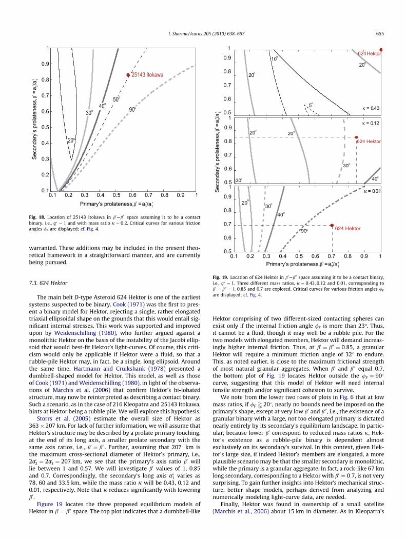
25143 Itokawa

20o

30o40o

90o

50o

0.9

0.1

0.2

0.3

0.4

0.5

0.6

0.7

0.8

1

0.90.1 0.2 0.3 0.4 0.5 0.6 0.7 0.8 1

Primary’s prolateness, ’ = a3’/a1’β

Seco

ndar

y’s

prol

aten

ess,

’ =

a 3’/a

1’β

Fig. 18. Location of 25143 Itokawa in b0—b00 space assuming it to be a contactbinary, i.e., q ¼ 1 and with mass ratio j ¼ 0:2. Critical curves for various frictionangles /F are displayed; cf. Fig. 4.

10o

20o

5o

624 Hektor

κ = 0.12

κ = 0.01

κ = 0.43

20o

30o

40o30o

624 Hektor

624 Hektor

30o

40o

90o

20o

20o

20o

0.9

0.5

0.6

0.7

0.8

1

0.9

0.5

0.6

0.7

0.8

1

0.9

0.5

0.6

0.7

0.8

1

0.90.1 0.2 0.3 0.4 0.5 0.6 0.7 0.8 1Primary’s prolateness, ’ = a3’/a1’β

Seco

ndar

y’s

prol

aten

ess,

’ =

a 3’/a

1’β

I. Sharma / Icarus 205 (2010) 638–657 655

warranted. These additions may be included in the present theo-retical framework in a straightforward manner, and are currentlybeing pursued.

Fig. 19. Location of 624 Hektor in b0—b00 space assuming it to be a contact binary,i.e., q ¼ 1. Three different mass ratios, j ¼ 0:43; 0:12 and 0.01, corresponding tob0 ¼ b00 ¼ 1; 0:85 and 0.7 are explored. Critical curves for various friction angles /F

are displayed; cf. Fig. 4.

7.3. 624 Hektor

The main belt D-type Asteroid 624 Hektor is one of the earliestsystems suspected to be binary. Cook (1971) was the first to pres-ent a binary model for Hektor, rejecting a single, rather elongatedtriaxial ellipsoidal shape on the grounds that this would entail sig-nificant internal stresses. This work was supported and improvedupon by Weidenschilling (1980), who further argued against amonolithic Hektor on the basis of the instability of the Jacobi ellip-soid that would best-fit Hektor’s light-curves. Of course, this criti-cism would only be applicable if Hektor were a fluid, so that arubble-pile Hektor may, in fact, be a single, long ellipsoid. Aroundthe same time, Hartmann and Cruikshank (1978) presented adumbbell-shaped model for Hektor. This model, as well as thoseof Cook (1971) and Weidenschilling (1980), in light of the observa-tions of Marchis et al. (2006) that confirm Hektor’s bi-lobatedstructure, may now be reinterpreted as describing a contact binary.Such a scenario, as in the case of 216 Kleopatra and 25143 Itokawa,hints at Hektor being a rubble pile. We will explore this hypothesis.

Storrs et al. (2005) estimate the overall size of Hektor as363� 207 km. For lack of further information, we will assume thatHektor’s structure may be described by a prolate primary touching,at the end of its long axis, a smaller prolate secondary with thesame axis ratios, i.e., b0 ¼ b00. Further, assuming that 207 km isthe maximum cross-sectional diameter of Hektor’s primary, i.e.,2a02 ¼ 2a03 ¼ 207 km, we see that the primary’s axis ratio b0 willlie between 1 and 0.57. We will investigate b0 values of 1, 0.85and 0.7. Correspondingly, the secondary’s long axis a001 varies as78, 60 and 33.5 km, while the mass ratio j will be 0.43, 0.12 and0.01, respectively. Note that j reduces significantly with loweringb0.

Figure 19 locates the three proposed equilibrium models ofHektor in b0 � b00 space. The top plot indicates that a dumbbell-like

Hektor comprising of two different-sized contacting spheres canexist only if the internal friction angle /F is more than 23�. Thus,it cannot be a fluid, though it may well be a rubble pile. For thetwo models with elongated members, Hektor will demand increas-ingly higher internal friction. Thus, at b0 ¼ b00 ¼ 0:85, a granularHektor will require a minimum friction angle of 32� to endure.This, as noted earlier, is close to the maximum frictional strengthof most natural granular aggregates. When b0 and b00 equal 0.7,the bottom plot of Fig. 19 locates Hektor outside the /F ¼ 90

curve, suggesting that this model of Hektor will need internaltensile strength and/or significant cohesion to survive.

We note from the lower two rows of plots in Fig. 6 that at lowmass ratios, if /F ’ 20, nearly no bounds need be imposed on theprimary’s shape, except at very low b0 and b00, i.e., the existence of agranular binary with a large, not too elongated primary is dictatednearly entirely by its secondary’s equilibrium landscape. In partic-ular, because lower b0 correspond to reduced mass ratios j, Hek-tor’s existence as a rubble-pile binary is dependent almostexclusively on its secondary’s survival. In this context, given Hek-tor’s large size, if indeed Hektor’s members are elongated, a moreplausible scenario may be that the smaller secondary is monolithic,while the primary is a granular aggregate. In fact, a rock-like 67 kmlong secondary, corresponding to a Hektor with b0 ¼ 0:7, is not verysurprising. To gain further insights into Hektor’s mechanical struc-ture, better shape models, perhaps derived from analyzing andnumerically modeling light-curve data, are needed.

Finally, Hektor was found in ownership of a small satellite(Marchis et al., 2006) about 15 km in diameter. As in Kleopatra’s

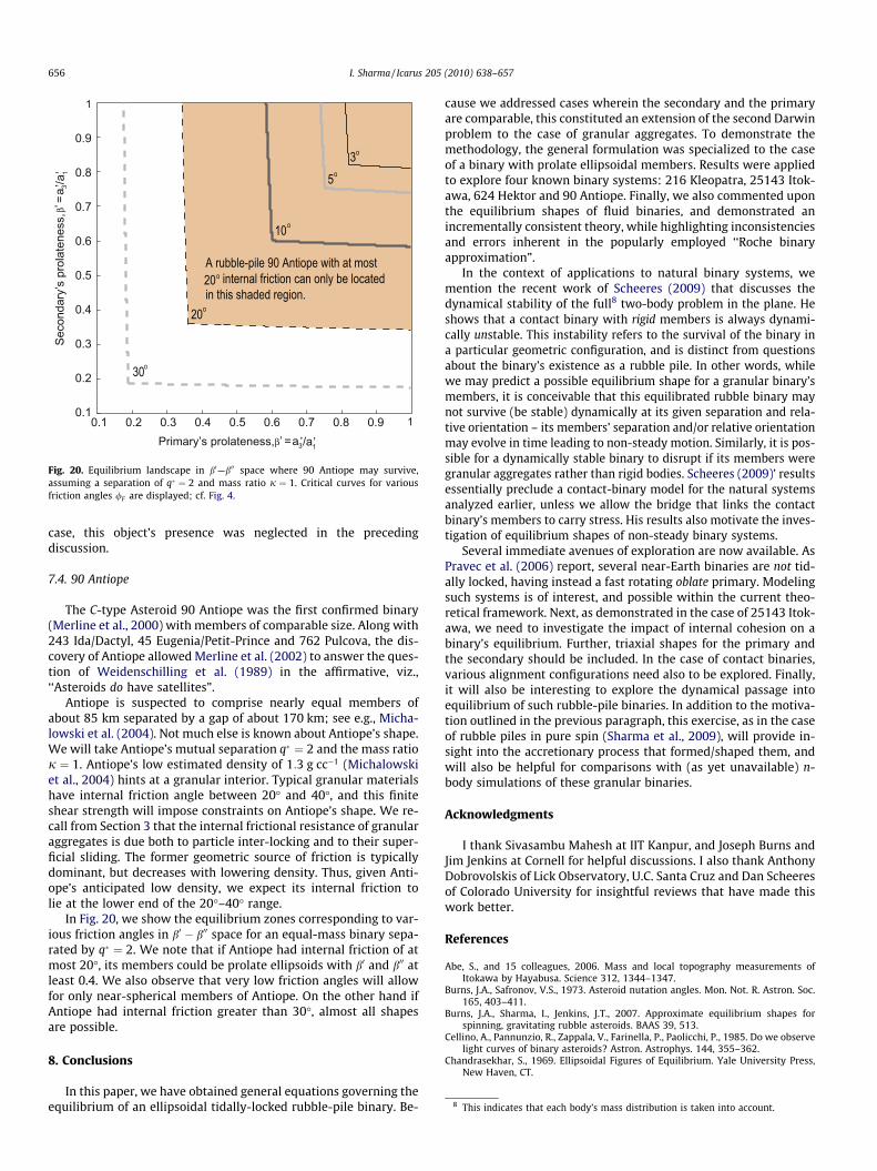
20o

30o

10o

5o

3o

A rubble-pile 90 Antiope with at most20o internal friction can only be located in this shaded region.

0.9

0.1

0.2

0.3

0.4

0.5

0.6

0.7

0.8

1

0.90.1 0.2 0.3 0.4 0.5 0.6 0.7 0.8 1

Primary’s prolateness, ’ = a3’/a1’β

Seco

ndar

y’s

prol

aten

ess,

’ =

a 3’/a

1’β

Fig. 20. Equilibrium landscape in b0—b00 space where 90 Antiope may survive,assuming a separation of q ¼ 2 and mass ratio j ¼ 1. Critical curves for variousfriction angles /F are displayed; cf. Fig. 4.

8 This indicates that each body’s mass distribution is taken into account.

656 I. Sharma / Icarus 205 (2010) 638–657

case, this object’s presence was neglected in the precedingdiscussion.

7.4. 90 Antiope

The C-type Asteroid 90 Antiope was the first confirmed binary(Merline et al., 2000) with members of comparable size. Along with243 Ida/Dactyl, 45 Eugenia/Petit-Prince and 762 Pulcova, the dis-covery of Antiope allowed Merline et al. (2002) to answer the ques-tion of Weidenschilling et al. (1989) in the affirmative, viz.,‘‘Asteroids do have satellites”.

Antiope is suspected to comprise nearly equal members ofabout 85 km separated by a gap of about 170 km; see e.g., Micha-lowski et al. (2004). Not much else is known about Antiope’s shape.We will take Antiope’s mutual separation q ¼ 2 and the mass ratioj ¼ 1. Antiope’s low estimated density of 1:3 g cc�1 (Michalowskiet al., 2004) hints at a granular interior. Typical granular materialshave internal friction angle between 20� and 40�, and this finiteshear strength will impose constraints on Antiope’s shape. We re-call from Section 3 that the internal frictional resistance of granularaggregates is due both to particle inter-locking and to their super-ficial sliding. The former geometric source of friction is typicallydominant, but decreases with lowering density. Thus, given Anti-ope’s anticipated low density, we expect its internal friction tolie at the lower end of the 20�–40� range.

In Fig. 20, we show the equilibrium zones corresponding to var-ious friction angles in b0 � b00 space for an equal-mass binary sepa-rated by q ¼ 2. We note that if Antiope had internal friction of atmost 20�, its members could be prolate ellipsoids with b0 and b00 atleast 0.4. We also observe that very low friction angles will allowfor only near-spherical members of Antiope. On the other hand ifAntiope had internal friction greater than 30�, almost all shapesare possible.

8. Conclusions

In this paper, we have obtained general equations governing theequilibrium of an ellipsoidal tidally-locked rubble-pile binary. Be-

cause we addressed cases wherein the secondary and the primaryare comparable, this constituted an extension of the second Darwinproblem to the case of granular aggregates. To demonstrate themethodology, the general formulation was specialized to the caseof a binary with prolate ellipsoidal members. Results were appliedto explore four known binary systems: 216 Kleopatra, 25143 Itok-awa, 624 Hektor and 90 Antiope. Finally, we also commented uponthe equilibrium shapes of fluid binaries, and demonstrated anincrementally consistent theory, while highlighting inconsistenciesand errors inherent in the popularly employed ‘‘Roche binaryapproximation”.

In the context of applications to natural binary systems, wemention the recent work of Scheeres (2009) that discusses thedynamical stability of the full8 two-body problem in the plane. Heshows that a contact binary with rigid members is always dynami-cally unstable. This instability refers to the survival of the binary ina particular geometric configuration, and is distinct from questionsabout the binary’s existence as a rubble pile. In other words, whilewe may predict a possible equilibrium shape for a granular binary’smembers, it is conceivable that this equilibrated rubble binary maynot survive (be stable) dynamically at its given separation and rela-tive orientation – its members’ separation and/or relative orientationmay evolve in time leading to non-steady motion. Similarly, it is pos-sible for a dynamically stable binary to disrupt if its members weregranular aggregates rather than rigid bodies. Scheeres (2009)’ resultsessentially preclude a contact-binary model for the natural systemsanalyzed earlier, unless we allow the bridge that links the contactbinary’s members to carry stress. His results also motivate the inves-tigation of equilibrium shapes of non-steady binary systems.

Several immediate avenues of exploration are now available. AsPravec et al. (2006) report, several near-Earth binaries are not tid-ally locked, having instead a fast rotating oblate primary. Modelingsuch systems is of interest, and possible within the current theo-retical framework. Next, as demonstrated in the case of 25143 Itok-awa, we need to investigate the impact of internal cohesion on abinary’s equilibrium. Further, triaxial shapes for the primary andthe secondary should be included. In the case of contact binaries,various alignment configurations need also to be explored. Finally,it will also be interesting to explore the dynamical passage intoequilibrium of such rubble-pile binaries. In addition to the motiva-tion outlined in the previous paragraph, this exercise, as in the caseof rubble piles in pure spin (Sharma et al., 2009), will provide in-sight into the accretionary process that formed/shaped them, andwill also be helpful for comparisons with (as yet unavailable) n-body simulations of these granular binaries.

Acknowledgments

I thank Sivasambu Mahesh at IIT Kanpur, and Joseph Burns andJim Jenkins at Cornell for helpful discussions. I also thank AnthonyDobrovolskis of Lick Observatory, U.C. Santa Cruz and Dan Scheeresof Colorado University for insightful reviews that have made thiswork better.

References

Abe, S., and 15 colleagues, 2006. Mass and local topography measurements ofItokawa by Hayabusa. Science 312, 1344–1347.

Burns, J.A., Safronov, V.S., 1973. Asteroid nutation angles. Mon. Not. R. Astron. Soc.165, 403–411.

Burns, J.A., Sharma, I., Jenkins, J.T., 2007. Approximate equilibrium shapes forspinning, gravitating rubble asteroids. BAAS 39, 513.

Cellino, A., Pannunzio, R., Zappala, V., Farinella, P., Paolicchi, P., 1985. Do we observelight curves of binary asteroids? Astron. Astrophys. 144, 355–362.

Chandrasekhar, S., 1969. Ellipsoidal Figures of Equilibrium. Yale University Press,New Haven, CT.

I. Sharma / Icarus 205 (2010) 638–657 657

Chen, W.F., Han, D.J., 1988. Plasticity for Structural Engineers. Springer-Verlag,New York.

Cook, A.F., 1971. 624 Hektor: A binary asteroid? In: T. Gehrels (Ed.), Physical Studiesof Minor Planets. NASA SP-267, pp. 155–163.

Darwin, G., 1906. On the figure and stability of a liquid satellite. Phil. Trans. R. Soc. A206, 161–248.

Demura, H., and 19 colleagues, 2006. Pole and global shape of 25143 Itokawa.Science 312, 1347–1349.

Descamps, P., 2008. Roche figures of doubly synchronous asteroids. Planet. SpaceSci. 56, 1839–1846.

Descamps, P., and 14 colleagues, 2007a. Nature of the small main belt Asteroid 3169Ostro. Icarus 189, 362–369.

Descamps, P., and 18 colleagues, 2007b. Figure of the double Asteroid 90 Antiopefrom adaptive optics and lightcurve observations. Icarus 187, 482–499.

Dobrovolskis, A.R., 1982. Internal stresses in Phobos and other triaxial bodies. Icarus52, 136–148.

Dobrovolskis, A.R., 1990. Tidal disruption of solid bodies. Icarus 88, 24–38.Fujiwara, A., and 21 colleagues, 2006. The rubble-pile asteroid Itokawa as observed

by Hayabusa. Science 312, 1330–1334.Fung, Y.C., 1965. Foundations of Solid Mechanics. Prentice-Hall, Englewood Cliffs,

NJ.Harris, A.W., Fahnestock, E.G., Pravec, P., 2009. On the shapes and spins of ‘‘rubble

pile” asteroids. Icarus 199, 310–318.Hartmann, W.K., Cruikshank, D.P., 1978. The nature of Trojan Asteroid 624 Hektor.

Icarus 36, 353–366.Hestroffer, D., Berthier, J., Descamps, P., Tanga, P., Cellino, A., Lattanzi, M.G., Di

Martino, M., Zappalà, V., 2002. 216 Kleopatra: Tests of the radar-derived shapemodel. Astron. Astrophys. 392, 729–733.

Holsapple, K.A., 2001. Equilibrium configurations of solid cohesionless bodies.Icarus 154, 432–448.

Holsapple, K.A., Michel, P., 2006. Tidal disruptions: A continuum theory for solidbodies. Icarus 183, 331–348.

Holsapple, K.A., Michel, P., 2008. Tidal disruptions II. A continuum theory for solidbodies with strength with applications to the Solar System. Icarus 193, 283–301.

Jeffreys, H., 1947. The relation of cohesion to Roche’s limit. Mon. Not. R. Astron. Soc.107, 260–262.

Knowles, J.K., 1998. Linear Vector Spaces and Cartesian Tensors. Oxford UniversityPress, Oxford. pp. 42–59.

Lacerda, P., Jewitt, D.C., 2007. Densities of Solar System objects from their rotationallight curves. Astron. J. 133, 1393–1408.

Leone, G., Farinella, P., Paolicchi, P., Zappalá, V., 1985. Equilibrium models of binaryasteroids. Astron. Astrophys. 140, 265–272.

Mann, R.K., Jewitt, D., Lacerda, P., 2007. Fraction of contact binary trojan asteroids.Astron. J. 134, 1133–1144.

Marchis, F., Berthierand, J., Wong, M.H., Descamps, P., Hestroffer, D., Colas, F., dePater, I., Vachier, F., 2006. Search of binary Jupiter-Trojan asteroids with laserguide star AO systems: A Moon around 624 Hektor. BAAS 38, 615.

Marchis, F., Descamps, P., Berthier, J., Emery, J.P., 2008. S/2008 (216) 1 and S/2008(216) 2. IAU Circ., 8980.

Marchis, F., Descamps, P., Berthier, J., Hestroffer, D., Vachier, F., Baek, M., Harris,A.W., Nesvorny, D., 2007. Main belt binary asteroidal systems with eccentricmutual orbits. Icarus 195, 295–316.

Marchis, F., Descamps, P., Hestroffer, D., Berthier, J., 2005. Discovery of the tripleasteroidal system 87 Sylvia. Nature 436, 822–824.

Merline, W.J., Close, L.M., Dumas, C., Shelton, J.C., Menard, F., Chapman, C.R., Slater,D.C., 2000. Discovery of companions to Asteroids 762 Pulcova and 90 Antiope bydirect imaging. BAAS 32, 1017.

Merline, W.J., Weidenschilling, S.J., Durda, D.D., Margot, J.-L., Pravec, P., Storrs, A.D.,2002. Asteroids do have satellites. In: Bottke, W.F., Jr., Cellino, A., Paolicchi, P.,Binzel, R.P. (Eds.), Asteroids III. University of Arizona Press, Tucson, AZ, pp. 289–312.

Michalowski, T., and 11 colleagues, 2004. Eclipsing binary Asteroid 90 Antiope.Astron. Astrophys. 423, 1159–1168.

Murray, C.D., Dermott, S.F., 1999. Solar System Dynamics. Cambridge UniversityPress, Cambridge. pp. 22–31.

Nedderman, R.M., 1992. Statics and Kinematics of Granular Materials. CambridgeUniversity Press, Cambridge.

Ostro, S.J., and 10 colleagues, 2005. Radar observations of Itokawa in 2004 andimproved shape estimation. Meteorit. Planet. Sci. 40, 1563–1752.

Ostro, S.J., and 15 colleagues, 2006. Radar imaging of binary near-Earth Asteroid(66391) 1999 KW4. Science 314, 1276–1280.

Ostro, S.J., Hudson, R.S., Nolan, M.C., Margot, J.-L., Scheeres, D.J., Campbell, D.B.,Magri, C., Giorgini, J.D., Yeomans, D.K., 2000. Radar observations of Asteroid 216Kleopatra. Science 288, 836–839.

Papadopoulos, P., 2001. On a class of higher-order pseudo-rigid bodies. Math. Mech.Solids 6, 631–640.

Pravec, P., and 56 colleagues, 2006. Photometric survey of binary near-Earthasteroids. Icarus 181, 63–93.

Richardson, D.C., Walsh, K.J., 2006. Binary minor planets. Annu. Rev. Earth Planet.Sci. 34, 47–81.

Saito, J., and 33 colleagues, 2006. Detailed images of Asteroid 25143 Itokawa fromHayabusa. Science 312, 1341–1344.

Scheeres, D.J., 2007. Rotational fission of contact binary asteroids. Icarus 189, 370–385.

Scheeres, D.J., 2009. Stability of the planar full 2-body problem. Celest. Mech. Dyn.Astr. 104, 103–128.

Scheirich, P., Pravec, P., 2009. Modeling of lightcurves of binary asteroids. Icarus200, 531–547.

Sharma, I., 2004. Rotational dynamics of deformable ellipsoids with applications toasteroids. Ph.D. thesis, Cornell University.

Sharma, I., 2009. The equilibrium of rubble-pile satellites: The Darwin and Rocheellipsoids for gravitationally held granular aggregates. Icarus 200, 636–654.

Sharma, I., Burns, J.A., Hui, C.-Y., 2005a. Nutational damping times in solids ofrevolution. Mon. Not. R. Astron. Soc. 359, 79–92.

Sharma, I., Jenkins, J.T., Burns, J.A., 2005b. Equilibrium configurations and the Rochelimit for spinning ellipsoidal soil-like asteroids. BAAS 37, 643.

Sharma, I., Jenkins, J.T., Burns, J.A., 2005c. Equilibrium shapes of ellipsoidal soilasteroids. In: García-Rojo, R., Hermann, H.J., McNamara, S. (Eds.), Proceedings ofthe 5th International Conference on Micromechanics of Granular Media, vol. 1.A.A. Balkema, pp. 429–432.

Sharma, I., Jenkins, J.T., Burns, J.A., 2006. Tidal encounters of ellipsoidal granularasteroids with planets. Icarus 183, 312–330.

Sharma, I., Jenkins, J.T., Burns, J.A., 2009. Dynamical passage to approximateequilibrium shapes for spinning, gravitating rubble asteroids. Icarus 200, 304–322.

Sheppard, S., Jewitt, D.C., 2004. Extreme Kuiper belt object 2001 QG298 and thefraction of contact binaries. Astron. J. 127, 3023–3033.

Spencer, A., 1980. Continuum Mechanics. Dover, New York. pp. 68–70.Storrs, A.D., Dunne, C., Conan, J.-M., Mugnier, L., Weiss, B.P., Zellner, B., 2005. A

closer look at main belt asteroids 1: WF/PC images. Icarus 173, 409–416.Takahashi, S., Shinokawa, K., Yoshida, F., Mukai, T., Ip, W.H., Kawabata, K., 2004.

Photometric and polarimetric observations and model simulations of (216)Kleopatra. Earth Planets Space 56, 997–1004.

Tanga, P., Hestroffer, D., Berthier, J., Cellino, A., Lattanzi, M.G., Di Martino, M.,Zappala, V., 2001. HST/FGS observations of the Asteroid (216) Kleopatra. Icarus153, 451–454.

Tanga, P., Hestroffer, D., Delbò, M., Richardson, D.C., 2009. Asteroid rotation andshapes from numerical simulations of gravitational re-accumulation. Planets.Space Sci. 57, 193–200.

Weidenschilling, S.J., 1980. Hektor: Nature and origin of a binary asteroid. Icarus 44,807–809.

Weidenschilling, S.J., Paolicchi, P., Zappala, V., 1989. Do asteroids have satellites? In:Binzel, R.P., Gehrels, T., Matthews, M.S. (Eds.), Asteroids II. University of ArizonaPress, Tucson, AZ, pp. 643–658.