1

Equilibrium of Interdependent Gas and ElectricityMarkets with Marginal Price Based Bilateral Energy

TradingCheng Wang, Wei Wei, Member, IEEE, Jianhui Wang, Senior Member, IEEE, Lei Wu, Senior Member, IEEE,

Yile Liang, Student Member, IEEE

Abstract— The increasing interdependencies between naturalgas systems and power systems create new business opportunitiesin coupled energy distribution markets. This paper studies themarginal price based bilateral energy trading on the equilibriumof coupled natural gas and electricity distribution markets.Convex relaxation is employed to solve a multi-period optimalpower flow problem, which is used to clear the electricity market.A successive second-order cone programming (SOCP) approachis utilized to solve a multi-period optimal gas flow problem,which is used to clear the gas market. In addition, the linepack effect in the gas network is considered, which can offerstorage capacity and provide extra operation flexibility for bothnetworks. In both problems, locational marginal energy prices arerecovered from the Lagrangian multipliers associated with nodalbalancing equations. Furthermore, a best-response decompositionalgorithm is developed to identify the equilibrium of the coupledenergy markets with bilateral gas and electricity trading, whichleverages the computational superiority of SOCPs. Cases studieson two test systems validate the proposed methodology.

Index Terms—interdependency, nodal energy price, natural gasnetwork, optimal energy flow, power distribution network.

NOMENCLATURE

A. Indices and Setsc ∈ C Gas compressors (gas active pipelines)dg ∈ Dg Gas distribution network (GDN) loadsdp ∈ Dp Power distribution network (PDN) loadsg ∈ G Gas-fired distributed generators (DGs)ig ∈ Ig GDN nodesip ∈ Ip PDN buseslg ∈ Lg Gas passive pipelineslp ∈ Lp PDN lines

This work is supported in part by the National Natural Science Foundationof China (51725702, 51627811), and in part by the ”111” project (B08013).W. Wei’s work is supported in part the Foundation for Innovative ResearchGroups of the National Natural Science Foundation of China (51621065). J.Wang’s work is supported by the U.S. Department of Energy (DOE)’s Officeof Electricity Delivery and Energy Reliability. L. Wu’s work is supportedin part by the U.S. National Science Foundation grant CMMI-1635339.(Corresponding to: Wei Wei)

C. Wang is with the State Key Laboratory of Alternate Electrical PowerSystem with Renewable Energy Sources, North China Electric Power Univer-sity, Beijing 102206, China (e-mail: chengwang@ncepu.edu.cn).

W. Wei and Y. Liang are with the State Key Laboratory of Power Systems,Department of Electrical Engineering, Tsinghua University, 100084 Beijing,China. (e-mail: wei-wei04@mails.tsinghua.edu.cn; yileat17@163.com)

J. Wang is with the Department of Electrical Engineering at South-ern Methodist University, Dallas, TX, USA and the Energy Systems Di-vision at Argonne National Laboratory, Argonne, IL, USA (email: jian-hui.wang@ieee.org).

L. Wu is with the Department of Electrical and Computer Engineering atClarkson University, Postdam, NY, 13699, USA. (e-mail: lwu@clarkson.edu).

n ∈ N Non-gas DGst ∈ T Time periodsφg Mapping between gas-fired DG and GDN nodeϕc Mapping between compressor and PDN node

B. ParameterseMlp PDN line current capacityFlg , Fc Pipeline friction coefficientsPLn /P

Mn Active power range of non-gas DGs

PLg /PMg Active power range of gas-fired DGs

aip/bip Shunt condunctance/susceptance from ip toground

Pdpt/Qdpt PDN active/reactive power demandsQLn/Q

Mn Reactive power range of non-gas DGs

QLg /QMg Reactive power range of gas-fired DGs

Qn(·) Generation cost of non-gas DGsRlg , Rc Pipe diametersrlp/xlp PDN line resistance/reactanceTk TemperaturevLip/v

Mip

PDN bus voltage magnitude rangeXlg , Xc Length of the pipelineYdgt GDN loadsybm Maximal allowed gas purchaseymaxc Maximal allowed gas in flow of compressorZlcrtg , Zc Compression factor of the pipelineαc Fuel consumption coefficient of compressorβipt Locational marginal electricity priceχ Thermal equivalent conversion constantηg Efficiency of gas-fired DGγc Compression factor of the compressorλgt Gas purchase price at a higher-level marketλpt Power purchase price at a higher-level marketµ Specific gas constantφlg Weymouth equation coefficientρ0 Gas density in standard conditionτuig/τ

lig

Gas pressure rangeθg Gas-electricity conversion factor%igt Locational marginal gas priceξ Unit transformation constant

C. Variableselpt Line current square of PDNmlgt,mct Average gas mass of GDNpbt/q

bt Purchased active/reactive power

pgt, pnt Active power of DGs

2

pflpt/qflpt Active/reactive power of PDN linesqgt, qnt Reactive power of DGsuigt Nodal gas pressureybt Purchased gasyinlgt/y

outlgt

Gas in/out-flow of passive pipelineyinct /y

outct Gas in/out-flow of active pipeline

νipt Bus voltage square of PDN

D. AcronymsCCP Convex concave procedureDG Distributed generatorGDN Gas distribution networkGTN Gas transmission networkLDC Local distribution companyLMP Locational marginal priceLMEP Locational marginal electricity priceLMGP Locational marginal gas priceLP Linear progMILP Mixed integer linear programmingOPF Optimal power flowOGF Optimal gas flowPDE Partial differential equationPDN Power distribution networkPTN Power transmission networkP2G Power-to-gasSOC Second-order coneSOCP Second-order cone programmingTLEM Transmission-level electricity marketTLGM Transmission-level gas market

I. INTRODUCTION

THe interdependencies between power and natural gassystems have been significantly enhanced during the past

decades, due to the proliferation of gas-fired generators inpower systems and the emerging power-to-gas (P2G) facilitiesin gas systems. Such increased interdependencies not onlybring potential economic and environmental benefits to thesociety, but also provide extra operating flexibility to bothcritical energy infrastructures. Many valuable works have beenfocused on the coordinated operation of coupled gas andpower systems. Just to name a few, the optimal gas-powerflow is studied in [1]; an interval optimization based robustdispatch model considering uncertain wind power and demandresponse is discussed in [2]; the coordinated system schedulingconsidering gas system dynamics is analyzed in [3]; a security-constrained co-planning model is presented in [4].

The wide deployment of gas-fired generators, gas com-pressors, and P2G facilities creates notable interdependenciesacross power systems and gas systems, as well as the marketsof both energy resources. On the one hand, the electricityprice will affect the gas production costs and delivery costs(because both the P2G facilities and the compressors aredriven by electricity), thus will further influence the elec-tricity demands from the gas side as well as the locationalmarginal gas prices (LMGPs), if a marginal pricing schemeis adopted in the gas market; on the other hand, the LMGPswill impact the production costs of the gas-fired generators,hence will influence the gas demands from the power grid

and the locational marginal electricity prices (LMEPs). Someinspiring works which endeavour to address the correlationbetween electricity and gas markets have been found. Theoptimal bidding problem of the gas-fired generators in the day-ahead electricity market considering the security constraintsof the gas network is discussed in [5] while neglecting theline pack effect, the quantity of natural gas contained in acertain segment of a pipeline [6]. [7] extends the work of [5]by taking unit commitment and wind power uncertainty intoaccount. In [8], the interdependency of power and gas systemsunder market environment in a medium-long time horizonis analyzed, where operation costs of individual systems areoptimized. Nevertheless, due to the existence of the nonlinearand nonconvex Weymouth equations, which are used forcapturing the mathematical relationship between gas flowsand pressures, pricing natural gas is still difficult, especiallywhen the marginal pricing scheme is adopted. The reason isthe nonconvexities will induce non-zero duality gap betweenthe primal and dual problems and the dual variables of thenodal energy balancing equation cannot be regarded as thelocational marginal prices (LMPs) directly. To conquer thisobstacle, [5] relaxes the Weymouth equation as an inequality,and then uses a series of linear inequalities to approximate therelaxed inequality, resulting in a linear form of the optimal gasflow (OGF) problem. However, this treatment cannot guaranteefeasibility of the OGF problem, which has been reported inliterature [9], making their work less attractive. Another possi-ble way is to add a series of binary variables and approximatethe Weymoth equation by a series of linear segments, turningthe gas market clearing problem into a mixed integer linearprogramming (MILP). It should be noted this approach hasbeen widely adopted in the coordinated operation issues ofgas-power system [10]–[14], yet hasn’t been reported by anygas pricing literature. However, the approximated gas flowmodel is still nonconvex, due to the introduction of binaries,which call for additional pricing schemes similar with theconvex hull pricing in power markets [15], [16].

Currently, the electricity and gas markets in the U.S. arecleared asynchronously [17] with different frequencies: theLMEPs are updated hourly, while the flat daily gas prices areprovided for certain users. For industrial gas-fired generators,they usually get the cheapest gas price with interruptiblesupply contracts, which may lead to fuel inadequacy if con-gestion or gas shortage occurs [18]. The wide adoption ofenergy transition facilities and increasingly prominent systeminterdependencies call for more reliable and resilient operationof both networks, and also create new business opportunitiesthat allow bilateral energy trading as well as promote the syn-chronization and coordination of electricity and gas markets,pioneered by the work in [17]. The first step for deregulatingthe gas network is to establish gas pricing policies and gasmarkets. We envision a pool-based gas market with LMGPswhich is similar to most existing power markets, becausemarginal pricing scheme has been well acknowledged for itsfairness and ability to price congestions. This paper studiesa coupled gas-electricity market of distribution networks withbilateral energy trading at locational marginal prices. Com-pared the existing works, the salient features of our work aresummarized as below.

3

1) We envision marginal gas pricing in the natural gas sys-tem. A convex optimization based method is proposed toclear the gas market and retrieve price, which overcomethe computational difficulty brought by the non-convexWeymouth equations.

2) To the best of our knowledge, it is the first time that sucha bilateral gas-electricity market is proposed, where thetwo markets trade energy at locational marginal prices.The proposed framework has the potential to promotegas and power system integration, and to increase theoperational flexibility of both systems. A best-responsedecomposition algorithm is suggested to compute theequilibrium of the coupled energy markets, and theexistence of equilibrium is discussed through the price-demand curves.

The rest of this paper is organized as follows. The marketframework and basic settings are clarified in Section II, follow-ing which the mathematical formulations of the power marketclearing and gas market clearing problems are elaborated.The solution methods for both market clearing problems, thecalculation of LMEPs and LMGPs, and the best responsealgorithm for the market equilibrium are introduced in SectionIII. To validate the proposed model and algorithm, numericalresults on two testing systems are presented in Section IV.Finally, conclusions are drawn in Section V.

II. MARKET FRAMEWORK, OPF AND OGF PROBLEMS

A. The Pool-based Market Framework

At the electricity side, the power distribution network (PDN)is connected with an upper-level power transmission network(PTN), and purchases electricity from it. Local generators inthe PDN include gas-fired and non-gas distributed generators(DGs). The PDN loads are deterministic. In the OPF problem,the electricity demands from compressors are treated as param-eters in the clearing process of the electricity market, whichare submitted by the gas system operator; natural gas is offeredat the LMGPs. The PDN operator clears the electricity marketwith minimal production costs, and determines the generationschedules, the gas demands, and the LMEPs simultaneously.

At the gas side, the gas distribution network (GDN) is con-nected with an upper-level gas transmission network (GTN),and purchases natural gas from it. The GDN loads are alsoconsidered deterministic. In the OGF problem, the naturalgas demands from gas-fired units are treated as parametersin the clearing process of the gas market, which are submittedby the power system operator; electricity is supplied at theLMEPs. The GDN operator clears the gas market with minimalproduction costs, and determines the gas transactions, thecompressor electricity usage, and the LMGPs simultaneously.The schematic diagram of the coupled energy markets isshown in Fig. 1.

The proposed market framework is designed for short-termoperation of the coupled energy networks, and the correspond-ing market clearing models are multi-period ones. For the day-ahead market, the time period could be 1 hour, and for theintra-day market, the time period could be 15 or 5 minutes.The adpativity of the market timeframe and length of a timeperiod can be achieved by adjusting the value of ξ, which is the

Electricity sources

q Power transmission network

q DGs

Electricity loads

q Internal loads

q External loads (compressors of GDN)

Gas sources

q Gas transmission network

Gas loads

q Internal loads

q External loads (Gas-fired DGs of PDN)

Electricity sourcesy

qq Power transmission networkPower transmissio

q DGs

Electricity loadsElectricity loadsElectricity loads

qq Internal loadsInternal loads

q External loads (compressors of GDN))

Gas sourcesGas sources

qq Gas transmission networkGas transm

Gas loadsGas loads

qq Internal loadsInternal l

q External loads (Gas-fired DGs of PDN)

Power distribution market Gas distribution market

LMEP LMGP

q External loads

Operation costsp

q Electricity purchase costs

q Gas purchase costs

q Non-gas generation costs

Operation costsOperation costs

q Electricity purchase costs

q Gas purchase costs

Market clearing Market clearing

Bilateral energy trading

GasElectricity

Fig. 1. The proposed coupled markets framework.

unit transformation constant. In the current work, the proposedmarket framework mainly focuses on energy trading, and theenergy transportation rights are not considered.

B. Assumptions and SimplificationsThe main assumptions made in the proposed optimal energy

flow models are clarified as follows.1) General assumptions: (i) We are focusing on the networks

and markets in the distribution level, where the PDN andthe GDN are operated with radial topologies, and energyflow directions can be determined in advance. (ii) The elec-tricity and gas consumptions are paid at locational marginalprices, i.e., the LMEPs and the LMGPs, respectively. (iii)P2G facilities are not considered in the proposed models forsimplicity. Technically, the proposed models can be easilyextended to ones with P2G facilities if linear P2G models areadopted [13], [19]. (iv) The PDN and GDN are owned andoperated by different local distribution companies (LDCs). Ifnot, the proposed bilateral energy trading market frameworkmay not work and no equilibrium exists, as there is only one“player” in the integrated energy market, suggesting a holisticoptimization model similar as the works of [1]–[4]. (v) Thedemands in both markets are non-elastic. For detailed price-responsive load model, one can refer to [20]. (vi) Only energytransactions with wholesale market are considered and thereis no retail market in the current work. Nonetheless, mostresults in this paper are easily extendable for transmission-level studies, despite a somehow different energy flow model.

2) For the PDN: (i) Electricity can be produced locally, orpurchased from the PTN at the contract prices. (ii) The branchflow model in [21] and the conic relaxation techniques in [22]are used. Reverse power flow is prohibited to guarantee thefeasibility of the optimal power flow (OPF) solution obtainedfrom the convexified model [23]–[25]. For controllable DGs,namely gas-fired DGs and diesel DGs, the assumption canbe easily satisfied due to their high operation flexibility. Forrenewable DGs, the assumption would still hold, if curtailmentis allowed. (iii) Gas demands of the gas-fired DGs solelydepend on their active power outputs. (iv) We assume that unitcommitment decisions have been made in a previous stage. Ifa DG is shut down, its output is enforced at zero. Interestedreaders can refer to [26] for the market clearing problemconsidering operating status of generators, however, this will

4

significantly intensifies the computation complexity. (v) DGsare assumed to be non-strategic, which means they offer theirgeneration costs as well as capacities to the power distributionmarket operator directly. (vi) The PDN is assumed to be abalanced one, and then the three-phase PDN model can bereplaced by an equivalent single-phase one. (vii) For each PDNnode equipped with one or several DGs, there exists at leastone combination of its downstream DGs, whose minimumoutputs is smaller than the sum of downstream demands of thesame PDN node. It should be noted the downstream DGs andloads of the PDN node include the ones connected to it if thereare any. To model an OPF of meshed transmission network,the direct current flow approximation or the traditional bus-injection model can be used. The former gives rise to a linearprogram, and the latter is nonlinear and non-convex, but canbe solved by the semi-definite relaxation method in [27].

3) For the GDN: (i) Gas flow dynamics are approximatedby algebraic equations. Details can be found in [11]. (ii) Asimplified and tractable compressor model in [6] is adopted,which can also be found in [10]–[13], [28], [29]. For thedetailed compressor model, please refer to [30]. Please notethat the accurate compressor modelling would impose greatchallenge on computation efficiency and model tractablity.Therefore, approximations and simiplifications in compressormodelling are quite common [10]–[14], [28], [29], [31]. Amore accurate and tractable compressor model in gas networkoptimization problems is desired. (iii) All the compressorsare driven by electricity and their cost functions are linear.According to [32] and [33], a compressor typically consumesabout 3-5% of the transported gas. Likewise, the compressorsare assumed to be non-strategic, which means they report theiroperating costs to the gas distribution market operator directly.

Remark 1: In this paper, the GDN is assumed to be operatedwith radial topology, which can be reasoned and supported bythe following factors.

1) Practicality. There are controllable valves in the GDN,which enables the GDN to be operated with radialtopology [34].

2) Efficiency. Radial-topology distribution networks enjoyhigh efficiency, especially in single source cases, as theirtotal lengths of the networks are smaller than those ofthe meshed ones [34], [35].

Radial-topology GDN analysis can be found in many lit-eratures [36]–[39], which further confirm the rationality ofthe proposed assumption. Nevertheless, the proposed modeland algorithm also apply to meshed network if gas flowdirections can be specified in advance from heuristic methodsor operating experiences. We do not actually require that gasflow directions keep unchanged all day long. In fact, gasflow problem is hard to solve for non-radial networks, evenunder steady-state and balanced conditions [40], due to thenonlinearities and nonconvexities in the gas network model,let along the OGF problem. Tractable pricing schemes for themeshed GDNs would be the one of the future works.

C. Power Distribution Market Clearing

The PDN is connected to a upper-level power transmissionnetwork (PTN), which serves as a power supplier with infinite

capacity. The PDN is a price-taker and pays the energytransaction costs to the transmission level electricity marketaccording to the electricity price. In the electricity market, theoperator aims to minimize the production costs, leading to thefollowing OPF problem

minΦp

∑t

(∑g

%igtpgt

ηgθg+∑n

Qn(pnt) + λptpbt), ig ∈ φ−1

g

Φp = {eipt, pbt , pgt, pnt, qbt , qgt, qnt, pflpt, qflpt, vipt}(1)

s.t. 0 ≤ elpt ≤ (eMlp )2, ∀lp,∀t, (2)

(vLip)2 ≤ νipt ≤ (vMip )2, ∀ip,∀t, (3)

PL{·} ≤ p{·}t ≤ PM{·}, {·} = {g, n},∀t, (4)

QL{·} ≤ q{·}t ≤ QM{·}, {·} = {g, n},∀t, (5)

pbt ≥ 0, qbt ≥ 0, ∀t, (6)

pflpt ≥ 0, qflpt ≥ 0,∀lp, t, (7)∑{·}∈Ψ{·}(ip)

p{·}t +∑

l∈ΨO2(ip)

(pflpt − rlpelpt)− aipνip

−∑

l∈ΨO1(ip)

pflpt −∑

dp∈Ψdp (ip)

Pdpt + 1{ip=i0p}pbt

−∑

c∈Ψc(ip)

χαcyinct = 0 : βipt, {·} = {g, n}, ∀ip, t,

(8)

∑{·}∈Ψ{·}(ip)

q{·}t +∑

l∈ΨO2(ip)

(qflpt − xlpelpt)− bipνip

−∑

l∈ΨO1(ip)

qflpt −∑

dp∈Ψdq (ip)

Qdqt + 1{ip=i0p}qbt

= 0, {·} = {g, n}, ∀ip, ∀t,

(9)

νip2t = νip1t − 2(rlppflpt + xlpqflpt)

+ (r2lp + x2

lp)elpt, ∀(ip1, ip2) ∈ lp,∀t,(10)

νip1telpt ≥ pf2lpt + qf2

lpt, ∀(ip1, ip2) ∈ lp,∀t. (11)

In this formulation, the objective function (1) is the totaloperating costs of the PDN, in which the first two componentsare the generation costs of gas-fired DGs and non-gas DGs,respectively, and the third one is the energy transaction costspaid to the transmission-level electricity market (TLEM); Φpcollects decision variables of the OPF problem. (2) and (3)impose boundaries for line currents and bus voltages. (4)and (5) enforce active and reactive generation capacities forDGs. (6) and (7) ban reverse energy transactions and powerflows, respectively. (8) and (9) are the nodal power balancingequations, where Ψg(ip), Ψn(ip), Ψdp(ip), and Ψc(ip) standfor sets of gas-fired DGs, non-gas DGs, electricity loads, andgas compressors connecting to node ip; ΨO1

(ΨO2) stands

for the set of feeders whose head (tail) node is ip; i0p isthe connection node between the upper-level PTN and PDN.(10) is the voltage drop equation. (11) defines the relaxedline apparent power, which can be expressed via a standardsecond-order cone constraint. It is proved that (11) will be

5

binding at the optimal solution under mild conditions [22].Dual variables which serve as the LMEPs are indicated in(8) following a colon. In the proposed market clearing modelof the PDN, renewable DGs, if there is any, use forecastedoutputs. Uncertainty is not the main focus of this paper, butwill be an interesting direction in future research. A relevantdiscussion is presented in Section III.C.

D. Gas Distribution Market Clearing

In the gas market, the operator aims to minimize the totalgas production costs, leading to the following OGF problem

minΦg

∑t

(λgtybt +

∑c

βiptχαcyinct ), ip ∈ ϕ−1

c ,

Φg = {ybt , yinlgt, youtlgt , y

inct , y

outct , uigt,mlgt}

(12)

s.t. 0 ≤ ybt ≤ ybm, ∀t, (13)

τ lig ≤ uigt ≤ τuig , ∀ig, t, (14)

1{ig=i0g}ybt +

∑{·}∈Θ{·}2 (ig)

yin{·}t −∑

{·}∈Θ{·}1 (ig)

yout{·}t =

∑n∈Θn(ig)

pgtηgθg

+∑

dg∈Θdg (ig)

Ydgt : %igt, {·} = {c, lg},∀ig, t,

(15)

m{·}t =π

4

X{·}R2{·}

µTkZ{·}ρ0

u{·}1t + u{·}2t

2, {·} = {c, lg}, ∀t,

(16)m{·}t = m{·}(t−1) + yin{·}t − y

out{·}t,

{·} = {c, lg}, t = 2, . . . , T,(17)

m{·}1 = m{·}T + yin{·}1 − yout{·}1, {·} = {c, lg}, (18)

uc2t ≤ γcuc1t, ∀c, t, (19)

0 ≤ yinct ≤ ymaxc , ∀c, t, (20)

(yinlgt + youtlgt )|yinlgt + youtlgt | = 4φlg [(ul1gt)2 − (ul2gt)

2], ∀lg, t,(21)

φlg =(π2ξ2R5

lg

)/(

16XlgFlgµTkZlgρ20

), ∀lg. (22)

In this formulation, the objective function (12) is the totaloperating costs of the GDN, in which the first component isthe gas purchase costs from the transmission-level gas market(TLGM), and the second one is the operating costs of compres-sors. Φg collects decision variables of the OGF problem. (13)prevents negative or excessive gas transactions. (14) imposesboundaries for nodal gas pressures. (15) represents nodal gasbalancing conditions, where Θdg (ig) and Θn(ig) represent setsof gas loads and gas-fired DGs connecting to node ig; Θc1(ig),Θc2(ig), Θlg1

(ig), and Θlg2(ig) represent sets of active and

passive pipelines whose head/tail node is ig . Particularly, ac-tive/passive pipelines refer to those with/without compressors;i0g denotes the connection node between the upper-level GTNand GDN. (16) gives the relationship between line pack andaverage pressure of a pipeline. (17) and (18) depict the time-dependent relationship between line pack and gas flow, andrequire the initial and final levels of line pack are the samein a clearing cycle. The mathematical procedure to derive

(16) and (17) can be found in the Appendix of [11], inwhich a constant compressibility factor Zlg is adopted topreserve linearity. For each active pipeline, (19) and (20)limit the maximum compression ratio and gas flow, whereuc1t and uc2t are the pressures of head and tail nodes of anactive pipeline, respectively. (19)-(20) constitute a simplifiedcompressor model, which has been justified and adopted in[6]. (21) is the Weymouth equation which characterizes therelationship between gas flow in a passive pipeline and nodalgas pressures, where ul1gt and ul2gt are pressures of head andtail nodes of lg , respectively. (22) defines the coefficient φlgin the Weymouth equation. Dual variables which serve as theLMGPs are indicated in (15) following a colon.

The non-differentiable absolute value function in (21)greatly challenges the solution of the OGF problem. Recallingthe first assumption of the general ones in Section II.A, (21)can be reduced as

ul1gt ≥ ul2gt, ∀lg, t, (23)

yinlgt + youtlgt ≥ 0, ∀lg, t, (24)

(yinlgt + youtlgt )2/4 = φlg ((ul1gt)2 − (ul2gt)

2), ∀lg, t. (25)

We assume the notations of head and tail nodes of lg areconsistent with the positive direction of gas flows. (23)-(25)naturally hold for radial GDNs. The non-convexity in the OGFproblem originates from equation (25).

Remark 2: According to the literature [41], [42], thecycling periods of most gas storages are years or months,which are not inconsistent with the time scale of the OGFproblem tackled here. Besides, gas storages usually locate intransmission networks rather than distribution networks [42].Therefore, in the short operation of gas distribution networks,the line pack, defined as the short-term storage by [41], actsas the distributed gas storage facilities with limited regulationcapability compared with the transmission-level gas storages,which has been modelled and serves as the only gas storagein the proposed OGF model. With more interactions betweendistribution-level electricity and gas networks, there may bemore gas storage facilities in the GDN in the future. Thoughgas storage facilities are not considered in this work, it can beeasily incorporated in the OGF model and efficiently solvedby the proposed algorithm, if it is convex mathematically. Takethe simplified linear gas storage model in [2], [11]–[13] as anexample:

yins≤ yinst ≤ yins , ∀s, ∀t, (26a)

youts≤ youtst ≤ youts , ∀s, ∀t, (26b)

rs ≤ rst ≤ rs, ∀s, ∀t, (26c)

rst = rs,t−1 + yinst − youtst , ∀s, ∀t, (26d)

where s is the index for gas storages; yins

and yins (youts

andyouts ) are the lower and upper limits of in (out) rate of gasstorages, respectively; rs and rs are lower and upper limitsof stored gas; yinst , youtst , and rst are the in rate, out rate,and stored gas, respectively. In this formulation, (26a) and(26b) describe the limits for in and out rates of gas storages,respectively; (26c) imposes the boundaries for stored gas;(26d) represents the variation of stored gas. Accordingly, the

6

nodal gas balancing equation needs to be modified as follows

1{ig=i0g}ybt +

∑{·}∈Θ{·}2 (ig)

yin{·}t −∑

{·}∈Θ{·}1 (ig)

yout{·}t+∑s∈Θs(ig)

(youtst − yinst

)=

∑n∈Θn(ig)

pgtηgθg

+∑

dg∈Θdg (ig)

Ydgt,

{·} = {c, lg},∀ig, t.(27)

It should be noted that modeling gas storage as (26a)-(26d)will not change the mathematical property of the gas distri-bution market clearing problem, which means the proposedapproach would still work.

Remark 3: There is no imbalance charge when the totalgas supply exceeds or is less than the total gas demand in atime period in the current formulation, as constraints (17) and(18) are embedded in the proposed OGF formulation, whichenforce the initial and final line pack levels of a clearing cycleare the same. However, it would be interesting to treat the linepack as an individual market product and explore its pricingscheme.

Remark 4: The formulations of gas flows are expressedby partial differential equations (PDEs), as shown in the Ap-pendix of [11]. Then the implicit method of finite differencesis used to discretize these PDEs in time and space. In [11],the time and space steps are selected as one hour and thelength of the pipeline, respectively. Similarly, the current linepack model, namely (16)-(18), is an approximation of theactual one. One possible method to improve the accuracyof approximation without losing its linearity is reported in[43], which is achieved by introducing fictitious gas nodesin a pipeline and dividing one pipeline into several sub-pipelines spatially. Temporally, the approximation could alsobe enhanced by using smaller time steps for the line packmodel compared with the one for gas market clearing.

Remark 5: Weymouth equation is adopted to approximatethe gas flow in a pipeline, which is the same as [44]. Infact, Weymouth equation is widely adopted in transmission-level gas network analysis [5], [11], [13], while the pressurelevels of GDNs are lower than GTNs, which means theWeymouth equation might not be the most accurate formulafor distribution-level gas flow analysis. In fact, there are manyformulas to describe the gas flow in a pipeline, however, nonehas the complete acceptance of academia and industry [45].This is because of the effects of friction are difficult to quan-tify, resulting in formula variations in the literature. Therefore,more accurate and tractable formulations for distribution-levelgas flow analysis are desired.

Remark 6: According to current natural gas market reality,LMGPs stay unchanged during a gas day. In the proposed gasmarket model, we assume the real-time natural gas pricingmechanism is adopted. However, the proposed model can bein line with current natural gas market reality after addingthe nodal gas balancing equations (15) with respect to t andregarding the dual variable %ig of the following equation asLMGP.

∑t

(1{ig=i0g}y

bt +

∑{·}∈Θ{·}2 (ig)

yin{·}t −∑

{·}∈Θ{·}1 (ig)

yout{·}t

)=

∑t

( ∑n∈Θn(ig)

pgtηgθg

+∑

dg∈Θdg (ig)

Ydgt

): %ig , {·} = {c, lg},∀ig.

(28)

With the aforementioned modifications, the LMGPs of gasmarket will remain unchanged throughout a gas day.

III. SOLUTION METHODOLOGY

A. Locational Marginal Electricity Price

The compact form of the OPF problem is given by

minx

f>x+ %>F%xx (29a)

s.t. 0 ≤ C1x+ d1 +D1y : β, (29b)

||Aix+ bi||2 ≤ c>2,ix+ d2,i : δ,ω, i ∈ Lp, (29c)

where x is vector of decision variables in Φg;f ,F%x,C1,d1,D1,Ai, bi, c2,i, d2,i are coefficient matricescorresponding to (1)-(11); β, δ and ω are dual variables. Inproblem (29), y and % are constant electricity demands andLMGPs delivered from the GDN. The dual SOCP of (29) isgiven by

maxβ,δ,ω

− β>(d1 +D1y)> −∑i∈Lp

(δ>i bi + ωid2,i

)(30a)

s.t. f + F>%x% = C>1 β +∑i∈Lp

(A>i δi + c2,iωi

), (30b)

β ≥ 0, ‖δi‖2 ≤ ωi, ∀i ∈ Lp. (30c)

As long as the OPF problem (29) has a Slater point, strongduality holds, which means dual variable βipt is the LMEPat bus ip. Some commercial SOCP solvers, such as MOSEK,offers primal and dual optimal solutions at the same time, thuscan be used to procure the OPF solution and the LMEPs moreconveniently.

B. Locational Marginal Gas Price

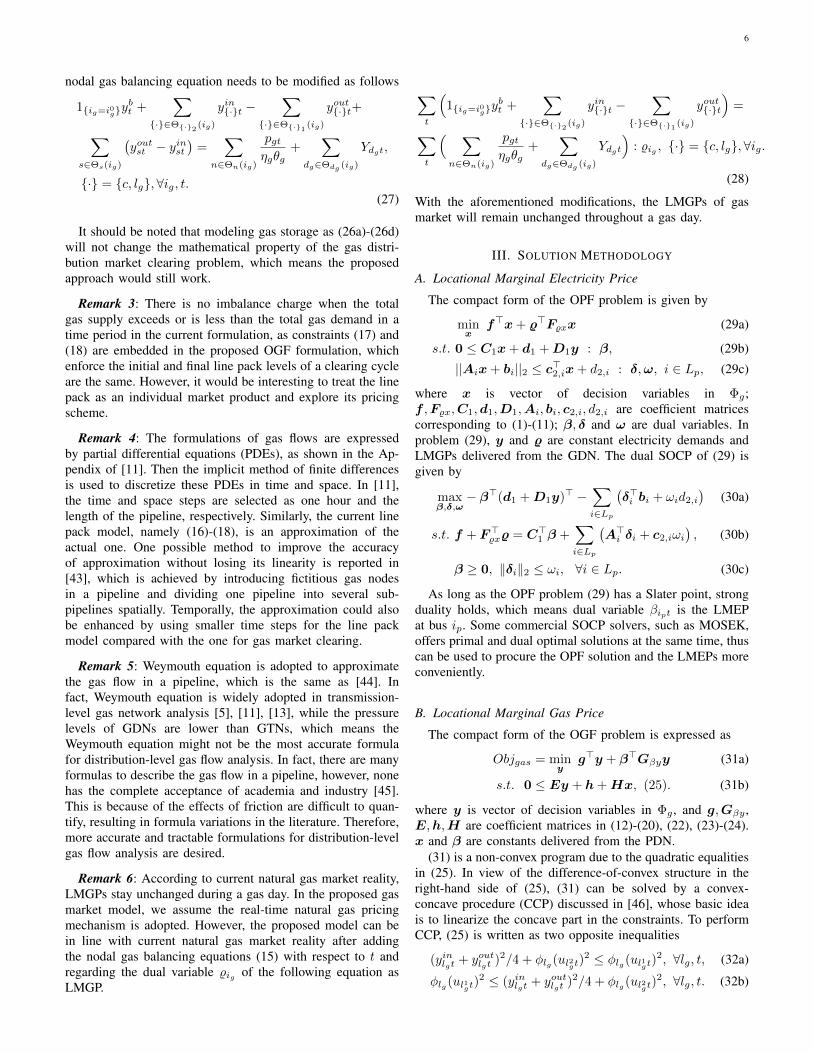
The compact form of the OGF problem is expressed as

Objgas = miny

g>y + β>Gβyy (31a)

s.t. 0 ≤ Ey + h+Hx, (25). (31b)

where y is vector of decision variables in Φg , and g,Gβy ,E,h,H are coefficient matrices in (12)-(20), (22), (23)-(24).x and β are constants delivered from the PDN.

(31) is a non-convex program due to the quadratic equalitiesin (25). In view of the difference-of-convex structure in theright-hand side of (25), (31) can be solved by a convex-concave procedure (CCP) discussed in [46], whose basic ideais to linearize the concave part in the constraints. To performCCP, (25) is written as two opposite inequalities

(yinlgt + youtlgt )2/4 + φlg (ul2gt)2 ≤ φlg (ul1gt)

2, ∀lg, t, (32a)

φlg (ul1gt)2 ≤ (yinlgt + youtlgt )2/4 + φlg (ul2gt)

2, ∀lg, t. (32b)

7

Algorithm 1 Penalty CCP for OGF1: Initialize the penalty parameters π0, πmax, κ > 1 and

convergence parameters δ and ε. Set the iteration indexk = 0. Solve the following relaxed OGF problem

Objgas = miny

g>y + β>Gβyy (36a)

s.t. 0 ≤ Ey + h+Hx, (33). (36b)

The optimal solutions (values) are y0 (Obj0gas).

2: Solve the following penalized OGF problem

Objgas = miny

g>y + β>Gβyy + πk1>s (37a)

s.t. 0 ≤ Ey + h+Hx, s ≥ 0, (33), (37b)

‖G1y + g1‖ ≤ g>2 y + g3, (37c)

where coefficient matrices G1, g1, g2, and g3 in SOCconstraint (37c) corresponding to (34) are updated at yk.The optimal solution is yk+1 and sk+1, with the optimalvalue of Objk+1

gas .3: If (38a) and (38b) are satisfied, then terminate and report

the optimal solution; otherwise, update k = k+1, πk+1 =min(κπk, πmax), and go to Step 2.

|Objk+1gas −Objkgas| ≤ δ, (38a)

slgt,k+1 ≤ ε · φlg (ul1gt)2, ∀lg, t. (38b)

Because ul1gt and φlg are positive,√φlgul1gt ≥ 0 holds, and

(32a) is equivalent to SOC inequalities shown below∥∥∥∥ (yinlgt + youtlgt)/2√

φlgul2gt

∥∥∥∥ ≤√φlgul1gt, ∀lg, t. (33)

Furthermore, given the value of ul2gt,k, yinlgt,k

and youtlgt,k,

(32b) can be convexified by replacing the right-hand side withits linear approximation, yielding

φlg (ul1gt)2 ≤

(yinlgt,k + youtlgt,k)(yinlgt + youtlgt

)

2− φlg (ul2gt,k)2

−(yinlgt,k + youtlgt,k

)2

4+ 2φlgul2gt,kul2gt, ∀lg, t.

(34)

Note that (34) is a set of convex quadratic inequalities and canbe further converted to second-order cone (SOC) inequalitiesas follows [47]

x2 ≤ by − d⇒

∥∥∥∥∥∥∥2x

y − b2√d

∥∥∥∥∥∥∥ ≤ y + b. (35)

To make the linear approximations performed in (34) com-patible, the nonnegative slack variable vector s as well as thepenalty term associated with s are incorporated in constraint(34) and objective (31a), respectively, rendering a penalizedversion of CCP shown in Algorithm 1, which is able to find alocal, but very promising to be the global, OGF solution. Theconvergence is proved in [46].

In Step 2 of Algorithm 1, problem (37), denoted as Mkg , is

solved in its SOCP form using the transforation in (35). While

Algorithm 2 Best-Response Decomposition1: Set %igt = λgt and yinct = 0. Set the maximum iteration

number jmax and convergence criterion ε. Set j = 1.2: Solve the OPF problem (29) with given yinct , %igt, and

obtain pjgt. Solve problem (30), and obtain LMEP βjipt.3: Solve the OGF problem (31) using Algorithm 1 with givenpjgt, β

jipt

, and obtain yin,jct ,Mk,jg . Solve the dual problem

of Mk,jg , and obtain LMGP %jigt.

4: If following criteria are met, terminate and report pjgt, βjipt

,yin,jct , %jigt; else if j = jmax, terminate and report failureof convergence; else, update j = j + 1, and go to Step 2.

|pjgt − pj−1gt | ≤ ε ·max{pjgt, p

j−1gt }, ∀g, t,

|βjipt − βj−1ipt| ≤ ε ·max{βjipt, β

j−1ipt}, ∀ip, t,

|yin,jct − yin,j−1ct | ≤ ε ·max{yin,jct , yin,j−1

ct }, ∀c, t,

|%jigt − %j−1igt| ≤ ε ·max{%jigt, %

j−1igt}, ∀ig, t.

Algorithm 1 converges, we solve the dual problem of Mkg in

the last iteration, which is again an SOCP, and recover dualvariables %igt as the LMGPs. The duality form of the SOCPis similar to (30) and is omitted here.

C. Market Equilibrium

Let OPF(LMGP, y) (OGF(LMEP, x)) be the OPF (OGF)problem with given LMGPs (LMEPs) and OGF (OPF) result y(x), the equilibrium of the market with bilateral gas-electricitytrading can come down to a fixed point problem

[LMEP,x] = OPF(LMGP,y)

[LMGP,y] = OGF(LMEP,x)(39)

The market interdependency originates from two observations:(i) the LMEPs (LMGPs), namely the dual variables of theOPF (OGF) problem, appear in the objective function of theOGF (OPF) problem; (ii) the gas (electricity) usage of gas-fired generators (compressors), i.e., the primal variables of theOPF (OGF) problem, appear in the constraints of the OGF(OPF) problem. A best-response decomposition algorithm isdesigned to identify the market equilibrium. Details are givenin Algorithm 2.

Remark 7: In fact, the proposed model and solution method-ology could extend to the cases with uncertain renewablesin the PDN. Currently, two major modeling approaches arewidely adopted in the power system operation problems withuncertain renewables, which are the scenario based stochasticapproach and the uncertainty set based robust one.

(1) Scenario based stochastic approach: if uncertainty ofrenewables is represented by scenarios, and the goal of oper-ator of the PDN is to minimize the expected operation costs,the compact form of the OPF problem would be a stochastic

8

programming as follows

minxj

∑j

πj

(f>xj +

(%j)>F%xx

j)

(40a)

s.t. 0 ≤ C1xj + d1 +D1y

j +M1uj : βj , ∀j, (40b)

||Aixj + bi||2 ≤ c>2,ixj + d2,i : δj ,ωj , i ∈ Lp, ∀j, (40c)

where j is scenario index and uj is outputs of the renewablesin scenario j; πj is probability of scenario j; xj is vectorof decision variables in scenario j; f , F%x, C1, d1, D1,M1, Ai, bi, c2,i, d2,i in model (40) are the same as model(29); M1 is the coefficient matrix for outputs of renewables;βj , δj and ωj are dual variables. In problem (40), yj and%j are constant electricity demands and LMGPs deliveredfrom the GDN. In (40), the objective (40a) is to minimizethe expected operation costs of the PDN, i.e., a weightedsum of the operation costs in each scenario; (40b) and (40c)are the PDN operation constraints in each scenario. With theintegration of renewables in the PDN, uncertainty will impactthe OGF problem indirectly, due to interdependencies betweenthe PDN and the GDN, leading to a stochastic formulation ofthe OGF problem as follows

minyj

∑j

πj

(g>yj +

(βj)>Gβyy

j)

(41a)

s.t. 0 ≤ Eyj + h+Hxj : %j , ∀j, (41b)(yj)>Qyj = 0, ∀j, (41c)

where yj is vector of decision variables in scenario j, andg,Gβy , E,h,H in (41) are the same as (31). xj and βj

are constants delivered from the PDN. In (41), the objective(40a) is to minimize the expected operation costs of the GDN,i.e., a weighted sum of the operation costs in each scenario;(41b)-(41c) are GDN operation constraints in each scenario.Specially, (41c) represents the nonlinear Weymouth equation.

However, it should be noted that the mathematical propertiesof the stochastic OPF and OGF models are the same with cor-responding deterministic ones, which are respectively SOCPsand quadratic equality constrained programmings. Therefore,the proposed solution approach would still work in this situa-tion.

(2) Uncertainty set based robust approach: if uncertaintyof renewables is represented by an uncertainty set, and thedecision goal of the PDN operator is to evaluate the “worst-case” operation costs, the OPF problem would be a max-minprogramming as below

maxu∈U

minx

f>x+ %>F%xx (42a)

s.t. 0 ≤ C1x+ d1 +D1y +M1u : β, (42b)

||Aix+ bi||2 ≤ c>2,ix+ d2,i : δ,ω, i ∈ Lp, (42c)

where u is outputs of renewables; U is the predetermineduncertainty set; other notations are the same as (29). Obvi-ously, (42) is not immediately solvable as it is a max-minprogramming. One widely adopted treatment is to take the dualof the inner level minimization problem, and then the bi-levelprogramming would degenerate to a single level maximizationproblem with bilinear terms in the objective function. Big-Mbased linearization approach in [48] can be applied and the

tractable reformulation is a mixed integer second-order coneprogramming (MISOCP), which can be solved by commercialsolvers such as Gurobi. Then the “worst-case” realization ofu can be obtained, denoted as u∗, and the LMEPs β can beretrieved by substituting u∗ into (29). It should be noted thatthe OGF problem will remain the same with (31), as bothdecision vector of PDN x and LMEPs β in the worst-caserealization of u are deterministic values rather uncertain ones.And it is not hard to tell that the proposed approach wouldstill work in this situation.

D. Discussions on the Existence of Market Equilibrium

Due to the complicated mathematical structure of the marketequilibrium problem, provable convergence guarantee of Al-gorithm 2 is non-trivial. We provide some intuitive discussionsto explain under what conditions Algorithm 2 is likely toconverge or may fail to converge. Our analysis rests on thenodal price-demand curves.

Consider a PDN node i∗p, which is connected with a gas-fired DG g∗, whose gas supply comes from GDN node i∗g .The relationship between the gas demand of g∗ and the gasprice at i∗g is illustrated by the grey curve in Fig. 2. While thegas price ρ is no larger than a certain value, say ρ ≤ ρ1, DGg∗ will keep working at its maximum generation capacity. Itis also easy to image that if % is greater than a certain value%2, g∗ might lose all the energy contract. When %1 ≤ % ≤ %2,the optimal generation of g∗ is likely to be a continuouslydecreasing function in %. Continuity is indicated by the factthat the Pareto-front of feasible nodal injection region for aradial network is strictly convex due to network losses, whichis revealed in [49], [50].

Now we consider the price response from the GDN: theLMGP at node i∗g is a function of the gas demand of g∗, whichis plotted by black curves in Fig. 2. As mentioned before, theLMGPs can be decomposed into a purchase component whichdepends on the gas price at TLGM and a delivery componentwhich relies on the LMEP at the compressor bus. Both ofthem are non-decreasing. When the demand exceeds the linepack capacity, the compressor has to increase its output inorder to deliver more gas. As a result, the LMGP grows as theLMEP rises. However, the continuity of black curves dependson specific system data. If it is indeed continuous, it is verylikely to intersect with the grey one. The intersection interpretsthe fixed point. If it is discontinuous, an intersection point mayexist or may not exist, as illustrated in Fig. 2.

Similarly, we consider a GDN node with a compressor c∗,whose electricity is supplied by PDN bus i∗p. The relationshipbetween the electricity demand of c∗ and the LMEP at i∗p isportrayed by grey curves in Fig. 3. The demand of c∗ remainsunchanged as long as the value of LMEP βi∗p is either smallor large enough. Grey curves can be either continuous ordiscontinuous, depending on the data of the OGF problem.On the other hand, black curves in Fig. 3 depict the LMEP asa function of electricity demand of c∗. In general, an LMEPcurve would be discontinuous, because nodal price could beattributed to a number of factors, and any active inequalitymight introduce a sudden rise in the LMEP. Take the losslesspower transmission network for example, the nodal price is

9

Gas Price of ig*

Gas

Dem

and o

f g*

01 20 *

Dg*

Dg0

ρ

Demand response curve

Price response curve

Gas Price of ig*

Gas

Dem

and o

f g*

01 20 *

Dg*

Dg0

ρ

Demand response curve

Price response curve

Gas Price of ig*

Gas

Dem

and o

f g

*

01 20

Dg0

ρ

Demand response curve

Price response curve

Fig. 2. Illustration of gas price and gas demand curves.

known to be stepwise constant [51]. Fig. 3 demonstrates fourpossible outcomes. In each of the left two subfigures, the twocurves have an intersection, and the market equilibrium exists;in the right two subfigures, no equilibria exist.

From above discussions, it can be concluded that theexistence of market equilibrium is system dependent. If noequilibrium exists, Algorithm 2 will fail to converge. Incontinuous case, Algorithm 2 is very likely to converge andfind the equilibrium, regardless of the initial point; If either ofthe curves is discontinuous, the equilibrium may not exist.In addition, even if an equilibrium indeed exists, whetherAlgorithm 2 can converge depends on the selection of theinitial point.

IV. ILLUSTRATIVE EXAMPLE

In this section, we present numerical results on two testsystems to validate the proposed methods. All experimentsare performed on a laptop with Intel(R) Core(TM) 2 Duo 2.2GHz CPU and 4 GB memory. The proposed algorithms arecoded in MATLAB with YALMIP toolbox [52]. SOCPs aresolved by Gurobi 6.5.

Fig. 4 depicts the topology of the connected infrastructures,which will be referred to as the Power13Gas7 system lateron. The PDN has 2 gas-fired DGs and 8 electric loads. TheGDN possesses 2 compressors, 4 passive pipelines, and 6

Electricity Price of ip*

Ele

ctri

city

Dem

and

of c*

0

Dp*

Dp0

1 2*bp

D

Demand response curve

Price response curve

Electricity Price of ip*

Ele

ctri

city

Dem

and

of c*

0

Dp0

1 2

pDb

Demand response curve

Price response curve

Electricity Price of ip*

Ele

ctri

city

Dem

and

of c*

0

Dp0 (Dp*)

1b *pD

Demand response curve

Price response curve

Electricity Price of ip*

Ele

ctri

city

Dem

and

of c*

0

Dp0

1bp

D

Demand response curve

Price response curve

Fig. 3. Illustration of electricity price and electricity demand curves.

gas loads. In Fig. 4, P, PL, and DG with subscripts denoteelectrical buses, power loads, and DG units in the PDN,respectively; N,C,GL, and GLine with subscripts denotegas nodes, compressors, gas loads, and passive pipelines inGDN, respectively. Specially, the fuel of DG1 and DG2 aresupplied by GDN nodes N4 and N6, respectively. Electricalcompressors C1 and C2 are connected to PDN buses P3 andP8, respectively. The daily demand profiles and price forecastsin TLEM and TLGM are shown in Fig. 5 and Fig. 6. Otherdetailed system data are available in [53]. Hereinafter, we usethe million British thermal unit (MMBtu) as the unifying unitfor electricity and natural gas, i.e., 1MMBtu equals to thethermal energy of 28.3 Sm3 thorough burnt gas, or 293 kWhelectricity.

GL1

GL6

N4 N3

N6

N2

N1

N7N5

GTN

C1

C2

PL1

P1

P2

P3 P4P6 P5

P7 P10 P11P9 P8

P13 P12

PL2PL3

PL4 PL5PL8 PL7

DG1

DG2

PL6N4

N6

PTN

GL3

GL5

PL6

P3

P8

GL2

GL4

GLine1

GLine2

GLine3 GLine4

Fig. 4. Topology of the Power13Gas7 system.

10

4 8 1 2 1 6 2 0 2 4

5

1 0

1 5

2 0 A c t i v e L o a d R e a c t i v e L o a dElectricity Demand (MMBtu)

T ( h )

5 0

6 0

7 0

8 0 P T N P r i c e

PTN Price ($/MMBtu)

Fig. 5. Demand profile of the PDN and the price curve in the TLEM.

4 8 1 2 1 6 2 0 2 41 5

2 0

2 5

3 0 G a s L o a d

Gas Demand (MMBtu)

T ( h )

1 0

2 0

3 0

4 0 G T N P r i c e

GTN Price ($/MMBtu)

Fig. 6. Demand profile of the GDN and the price curve in the TLGM.

A. Simulation Results of the Base Case

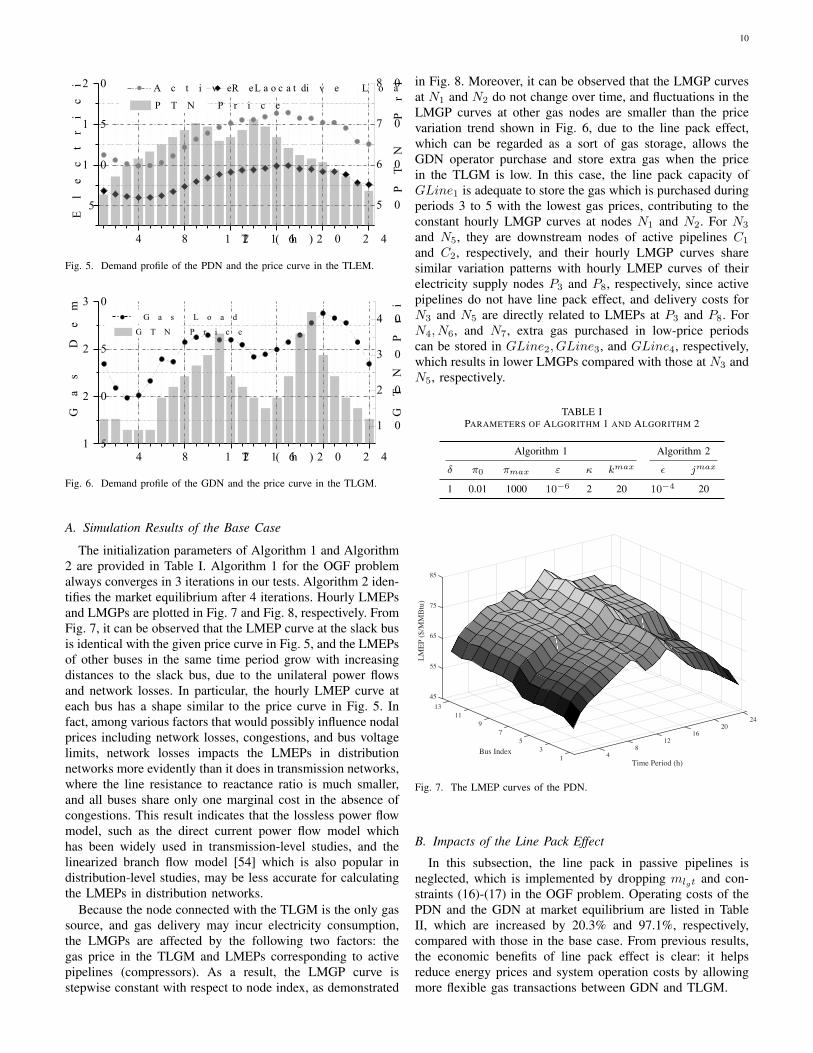
The initialization parameters of Algorithm 1 and Algorithm2 are provided in Table I. Algorithm 1 for the OGF problemalways converges in 3 iterations in our tests. Algorithm 2 iden-tifies the market equilibrium after 4 iterations. Hourly LMEPsand LMGPs are plotted in Fig. 7 and Fig. 8, respectively. FromFig. 7, it can be observed that the LMEP curve at the slack busis identical with the given price curve in Fig. 5, and the LMEPsof other buses in the same time period grow with increasingdistances to the slack bus, due to the unilateral power flowsand network losses. In particular, the hourly LMEP curve ateach bus has a shape similar to the price curve in Fig. 5. Infact, among various factors that would possibly influence nodalprices including network losses, congestions, and bus voltagelimits, network losses impacts the LMEPs in distributionnetworks more evidently than it does in transmission networks,where the line resistance to reactance ratio is much smaller,and all buses share only one marginal cost in the absence ofcongestions. This result indicates that the lossless power flowmodel, such as the direct current power flow model whichhas been widely used in transmission-level studies, and thelinearized branch flow model [54] which is also popular indistribution-level studies, may be less accurate for calculatingthe LMEPs in distribution networks.

Because the node connected with the TLGM is the only gassource, and gas delivery may incur electricity consumption,the LMGPs are affected by the following two factors: thegas price in the TLGM and LMEPs corresponding to activepipelines (compressors). As a result, the LMGP curve isstepwise constant with respect to node index, as demonstrated

in Fig. 8. Moreover, it can be observed that the LMGP curvesat N1 and N2 do not change over time, and fluctuations in theLMGP curves at other gas nodes are smaller than the pricevariation trend shown in Fig. 6, due to the line pack effect,which can be regarded as a sort of gas storage, allows theGDN operator purchase and store extra gas when the pricein the TLGM is low. In this case, the line pack capacity ofGLine1 is adequate to store the gas which is purchased duringperiods 3 to 5 with the lowest gas prices, contributing to theconstant hourly LMGP curves at nodes N1 and N2. For N3

and N5, they are downstream nodes of active pipelines C1

and C2, respectively, and their hourly LMGP curves sharesimilar variation patterns with hourly LMEP curves of theirelectricity supply nodes P3 and P8, respectively, since activepipelines do not have line pack effect, and delivery costs forN3 and N5 are directly related to LMEPs at P3 and P8. ForN4, N6, and N7, extra gas purchased in low-price periodscan be stored in GLine2, GLine3, and GLine4, respectively,which results in lower LMGPs compared with those at N3 andN5, respectively.

TABLE IPARAMETERS OF ALGORITHM 1 AND ALGORITHM 2

Algorithm 1 Algorithm 2

δ π0 πmax ε κ kmax ε jmax

1 0.01 1000 10−6 2 20 10−4 20

2420

16

Time Period (h)

128

413

5Bus Index

79

1113

85

75

65

55

45

LMEP

($/M

MB

tu)

Fig. 7. The LMEP curves of the PDN.

B. Impacts of the Line Pack Effect

In this subsection, the line pack in passive pipelines isneglected, which is implemented by dropping mlgt and con-straints (16)-(17) in the OGF problem. Operating costs of thePDN and the GDN at market equilibrium are listed in TableII, which are increased by 20.3% and 97.1%, respectively,compared with those in the base case. From previous results,the economic benefits of line pack effect is clear: it helpsreduce energy prices and system operation costs by allowingmore flexible gas transactions between GDN and TLGM.

11

2420

16

Time Period (h)

128

412

3

Node Index

45

67

18

15

12

9

6

LMG

P ($

/MM

Btu

)

Fig. 8. The LMGP curves of the GDN.

TABLE IIOPERATING COSTS AT EQUILIBRIUM WITH/WITHOUT LINE PACK

PDN ($) GDN ($)

With line pack 2.1505× 104 7.6052× 104

Without line pack 2.5871× 104 1.4990× 105

In fact, the line pack capacity in the pipelines are mainlydetermined by nodal pressure limits and parameters of thepipelines. And nodal pressure limits are crucial to both theoperating feasibility and flexibility of the GDN. From thefeasibility perspective, if the limits decrease, the maximumallowable gas flow through a pipeline would decrease si-multaneously, and if the limits are below certain thresholds,the nodal gas balancing equations would not hold, leadingto infeasibility issues of the OGF problem. And from theflexibility perspective, capacity of the line pack has a positiverelationship with pressures of head and tail nodes of a pipelineaccording to (16), which means it will drop correspondinglyif the pressure limits decrease. And of course the lowerline pack capacities are, the higher the operation costs ofboth energy distribution networks might be, indicating loweroperating flexibility of the GDN accordingly. To verify theaforementioned analysis, the simulations in Section IV.A arerepeated with different nodal pressure limits, and operationcosts of the two energy networks are displayed as follows

TABLE IIIOPERATING COSTS AT EQUILIBRIUM WITH DIFFERENT LEVELS OF NODAL

PRESSURE LIMITS.

Pressure (%) PDN ($) GDN ($)

100 2.1505× 104 7.6052× 104

80 2.2201× 104 8.3217× 104

60 2.3445× 104 9.7762× 104

40 2.5162× 104 1.2165× 105

20 - Infeasible

In Table III, the left column indicates pressure limits level,e.g., 80% means pressure limits of all nodes are 80% of thecorresponding values in the Power13Gas7 test system. FromTable III, it can be observed that operation costs of both

energy networks will increase along with the drop of pressurelimits. Specifically, when pressure limits drop to 20%, the OGFproblem would be infeasible.

C. Comparisons with other OGF Solution MethodsAs previously mentioned, the sequential SOCP algorithm

is proposed to solve the gas market clearing problem, whichidentifies a local, but very promising to be the global, OGFsolution. In fact, due to the nonlinearities and nonconvexitiesin the gas market clearing problem, the global optimality of thesolution cannot be theoretically guaranteed. However, it is stillworth comparing the quality of the solution obtained by theproposed algorithm with the ones obtained by other algorithmsand methods. To the best knowledge of the authors, threemethods to solve the nonlinear and nonconvex OGF problemhave been reported by the literature, which are

1) A1: MILP based method [10]–[14], where the nonlinearWeymouth equation is approximated by a series of linearsegments and nearly same amount of binary variables areadded, rendering an MILP approximation of the originalOGF problem.

2) A2: SOCP/ linear programming (LP) relaxation method[2], [5], where the Weymouth equation is relaxed asan SOCP inequality or a series of linear inequalities,transforming the nonconvex OGF problem into a convexone.

3) A3: Interior point method, which can obtain a solutionfor many nonlinear programming in a given time limit.It should be noted the initial point have direct impacton the quality of solution.

The gas network of the Power13Gas7 system is selected asthe test system for the OGF problem. The parameters can befound in [53]. The variables, which are related to the electricitynetwork and appear in the OGF problem, are parameterizedwith the OPF solution in the last iteration of Algorithm 2.In A1, two eight-segment piecewise linear approximations areadopted to replace the nonlinear Weymouth equation [11]. Totest the performance of A3 under different choices of initialpoint, A3 is performed 103 times with different initial points,including the OGF solution offered by A2, which is identicalwith the initial point of CCP. Particularly, MILPs are solvedby Gurobi 6.5 and the interior point method is from OPTItoolbox. The solution time limit is set as 10 minutes. Thesimulation results are summarized in Table IV, where F, Yand N are short for feasible, yes and no, respectively, in thefifth column.

TABLE IVCOMPARISON WITH THE STATE-OF-ART METHODOLOGIES FOR THE OGF

PROBLEM

Objective ($) F Time (s)avg max min

CCP 7.605× 104 - - Y 0.68A1 8.426× 104 - - Y 720∗

A2 7.405× 104 - - N 0.09A3 7.824× 104 8.294× 104 7.652× 104 Y 75

The comparisons are conducted in three aspects, namely, theOGF costs, the feasibility of the OGF solution, and the solution

12

time. It should be noted that, the results of CCP, A1, andA2 in Table IV refer to the single time performance of thesealgorithms, while the results of A3 is the average performanceof 103 tests. From Table IV, though the objective value of A2is the lowest, its OGF solution is infeasible. A1 can offera feasible solution, however, its computational burden is thelargest and the time runs out before an optimal solution isobtained. Among the algorithms which can offer a feasibleOGF solution, namely, CCP, A1 and A3, CCP performs thebest in terms of both objective value and solution time. Fromthe simulation results, it should be noted that OGF solutionoffered by CCP is always better than A3, including the bestcase of A3. In this regard, the OGF solution offered by theproposed CCP method is satisfying, which is the basis of an“optimal” equilibrium.

D. Impacts of Compressors

If the GDN in the couple energy networks does not havecompressor stations, the models and algorithms still work afterthe following modifications

1) In the PDN market clearing model, remove the activepower consumption terms of the compressor in the nodalactive power balance equation.

2) In the GDN market clearing model, remove the elec-tricity purchase cost terms in the objective function aswell as the compressor related terms and models in theconstraints.

3) In the proposed best-response decomposition algorithm,remove the compressor related convergence criterion.

To demonstrate the impact of compressors on the results,numerical tests are executed on the modified Power13Gas7system, where the compressors in the GDN have been re-moved, and the rest is the same as the Power13Gas7 systemdemonstrated in Section IV, including the daily electricitydemand profiles and price forecasts in the transmission-levelenergy markets. It should be noted that the OGF problemwould be infeasible without compressors, if the daily gasdemand profiles stay the same. Therefore, the gas demands areset as one third of the ones in [53] to recover the feasibilityof the OGF problem with no compressors equipped.

Likewise, Algorithm 1 for the OGF problem always con-verges in 3 iterations. And Algorithm 2 locates the marketequilibrium after 3 iterations, which converges faster than thecase in Section IV.A, because the bilateral energy tradingdegenerates to unilateral one, as a result, the interdependencyis weakened. Hourly LMGPs are shown in Fig. 9. From Fig.9, it can be observed that the LMGPs remain unchangedthroughout the day, and their values are 9 $/MMBtu, whichis the lowest price of TLGM. The reason is that the GDNoperation costs only consist of the gas purchase costs fromthe GTN as there is no compressors, and the pipelines arecapable to store adequate gas when the price is low. Thoughthe LMGPs have decreased dramatically compared with thecase in Section IV.A, the LMEP curves in this case share thesame trends as Fig.7. This is because the total capacity ofDGs in the PDN is always smaller than its hourly electricitydemand, which indicates the PDN has to buy electricity fromthe PTN invariably in both cases. In the case of Section IV.A,

PTN is the marginal “generator”, as its price is the higher thanthe DGs. In this case, the generation costs of DGs decreaseas the LMGPs decrease, which means the PTN is still themarginal “generator”, resulting in the same variation trends inthe LMEP curves of the two cases.

LMG

P ($

/MM

Btu

)

6

9

12

Time Period (h)4

812

1620

24

Node Index 12

34

56

7

Fig. 9. The LMGP curves of the GDN with no compressors equipped.

E. Computational Efficiency Analysis

To demonstrate the scalability and efficiency of the proposedmethods, they are applied to a larger system, consistingof a modified IEEE 123-bus power feeder and a modifiedBelgian high-calorific 20-node gas network, which will bereferred to as the Power123Gas20 system hereinafter. Thesystem includes 10 gas-fired DGs, 3 compressors, 16 passivepipelines, 85 power loads, and 9 gas loads. Please refer to[53] for the network topology, the demand curves as well asother system data. Algorithmic parameters in Table I are usedin this case.

The convergence performances are shown in Fig. 10. It canbe observed that both algorithms converge in 3 iterations. Thetotal computation time of Algorithm 1 and Algorithm 2 is 7.24seconds, demonstrating the scalability of the proposed meth-ods. Besides the satisfactory convergence rates of Algorithms1-2, the high efficiency is also attributed to the computationalsuperiority of SOCPs, which can be readily solved even forvery large-scale instances [47].

V. CONCLUSION

The interdependencies between power systems and gas sys-tems have been greatly enhanced in recent decades, indicatinga greater amount of bilateral energy flows as well as morebusiness opportunities. In this paper, a market frameworkfor the coupled power and gas distribution systems, bothwith radial topologies, is designed, which allows the energymarkets to trade energy bilaterally with its marginal price.Under certain assumptions and simplifications, the multi-period alternating current OPF problem becomes tractable us-ing convex relaxation techniques. The penalty CCP algorithmis developed to turn the nonlinear and nonconvex multi-periodOGF problem with the line pack effect into a tractable one,

13

1 2 30.0

0.1

0.2

0.3

LMEP Gap

LMGP Gap

Rel

ativ

e G

ap

Iteration Number: A2

1 2 30.0

0.2

0.4

0.6

0.8

1.0

Objective Gap

Slack Gap

Rel

ativ

e G

ap

Iteration Number: A1, j=1

1 2 30.0

0.2

0.4

0.6

0.8

1.0

Objective Gap

Slack Gap

Rel

ativ

e G

ap

Iteration Number: A1, j=21 2 3

0.0

0.2

0.4

0.6

0.8

1.0

Objective Gap

Slack Gap

Rel

ativ

e G

ap

Iteration Number: A1, j=3

Fig. 10. Algorithm performances in the Power123Gas20 system.

where a sequence of convex optimization problems is tackled.SOCP based methods are used to solve the OPF problemand the OGF problem, as well as to recover the locationalmarginal energy prices. A best-response decomposition algo-rithm is developed to identify the market equilibrium, whoseexistence is analytically investigated via nodal price-demandcurves. Simulation results corroborate the effectiveness of theproposed methods, and reveal economic benefits of the linepack effect. Two promising aspects are selected as our futureresearch interests and listed as below, which could facilitatethe application of the proposed market framework.

1) More accurate and tractable gas network modelling.Detailed compressor models would be considered. Theaccuracies of the approximation techniques for the gasflows and their dynamics need to be improved.

2) More reliable algorithm for market equilibrium identifi-cation. Particularly, a criterion for the existence of themarket equilibrium needs to be developed.

ACKNOWLEDGMENT

The authors would like to thank the editor and six anony-mous reviewers for their valuable and inspiring suggestions toimprove the quality of the paper.

REFERENCES

[1] A. Martinez-Mares and C. Fuerte-Esquivel, “A unified gas and powerflow analysis in natural gas and electricity coupled networks,” IEEETrans. Power Syst., vol. 27, no. 4, pp. 2156–2166, Nov. 2012.

[2] L. Bai, F. Li, H. Cui, T. Jiang, H. Sun, and J. Zhu, “Interval optimizationbased operating strategy for gas-electricity integrated energy systemsconsidering demand response and wind uncertainty,” Appl. Energy, vol.167, pp. 270–279, Apr. 2016.

[3] C. Liu, M. Shahidehpour, and J. Wang, “Coordinated scheduling ofelectricity and natural gas infrastructures with a transient model fornatural gas flow,” Chaos: An Interdisciplinary Journal of NonlinearScience, vol. 21, no. 2, p. 21052, 2011.

[4] X. Zhang, M. Shahidehpour, A. Alabdulwahab, and A. Abusorrah,“Security-constrained co-optimization planning of electricity and naturalgas transportation infrastructures,” IEEE Trans. Power Syst., vol. 30,no. 6, pp. 2984–2993, Nov. 2015.

[5] H. Cui, F. Li, Q. Hu, L. Bai, and X. Fang, “Day-ahead coordinatedoperation of utility-scale electricity and natural gas networks consideringdemand response based virtual power plants,” Appl. Energy, vol. 6, pp.183–195, Aug. 2016.

[6] A. Tomasgard, F. Rmo, M. Fodstad, and K. Midthun, “OptimizationModels for the Natural Gas Value Chain,” in Geometric Modelling, Nu-merical Simulation, and Optimization: Applied Mathematics at SINTEF.Berlin, Heidelberg: Springer, 2007, pp. 521–558.

[7] R. Chen, J. Wang, and H. Sun. (2016) Clearing and pricing forcoordinated gas and electricity day-ahead markets considering windpower uncertainty. [Online]. Available: https://arxiv.org/abs/1611.09599

[8] M. Gil, P. Duenas, and J. Reneses, “Electricity and natural gas interde-pendency: comparision of two methodologies for coupling large marketmodels within the european regulatory framework,” IEEE Trans. PowerSyst., vol. 31, no. 1, pp. 361–369, Jan. 2016.

[9] C. Wang, W. Wei, J. Wang, L. Bai, Y. Liang, and T. Bi, “Convexoptimization based distributed optimal gas-power flow calculation,”IEEE Trans. Sustain. Ener., vol. PP, no. 99, pp. 1–1, 2017.

[10] C. M. Correa-Posada and P. Snchez-Martn, “Security-constrained op-timal power and natural-gas flow,” IEEE Trans. Power Syst., vol. 29,no. 4, pp. 1780–1787, July 2014.

[11] C. Correa-Posada and P. Sanchez-Martin, “Integrated power and naturalgas model for energy adequacy in short-term operation,” IEEE Trans.Power Syst., vol. 30, no. 6, pp. 3347–3355, Nov. 2015.

[12] C. Wang, W. Wei, J. Wang, F. Liu, F. Qiu, C. M. Correa-Posada,and S. Mei, “Robust defense strategy for gas-electric systems againstmalicious attacks,” IEEE Trans. Power Syst., vol. 32, no. 4, pp. 2953–2965, July 2017.

[13] C. He, L. Wu, T. Liu, and M. Shahidehpour, “Robust co-optimizationscheduling of electricity and natural gas systems via ADMM,” IEEETrans. Sustain. Ener., vol. 8, no. 2, pp. 658–670, 2017.

[14] C. Shao, X. Wang, M. Shahidehpour, X. Wang, and B. Wang, “An milp-based optimal power flow in multicarrier energy systems,” IEEE Trans.Sustain. Ener., vol. 8, no. 1, pp. 239–248, Jan 2017.

[15] D. A. Schiro, T. Zheng, F. Zhao, and E. Litvinov, “Convex hullpricing in electricity markets: Formulation, analysis, and implementationchallenges,” IEEE Trans. Power Syst., vol. 31, no. 5, pp. 4068–4075, Sep2016.

[16] B. Hua and R. Baldick, “A convex primal formulation for convex hullpricing,” IEEE Trans. Power Syst., vol. 32, no. 5, pp. 3814–3823, Sep.2017.

[17] P. Weigand, G. Lander, and R. Malme, “Synchronizing natural gas &power market: a series of proposed solutions,” Skipping Stone, Tech.Rep., Jan. 2013.

[18] “Analysis of operational events and market impacts during the january2014 cold weather events,” PJM Interconnection, Tech. Rep., May 2014.

[19] G. Li, R. Zhang, T. Jiang, H. Chen, L. Bai, and X. Li, “Security-constrained bi-level economic dispatch model for integrated naturalgas and electricity systems considering wind power and power-to-gasprocess,” Appl. Energy, vol. 194, pp. 696–704, May 2017.

[20] C. Ruiz, A. J. Conejo, and Y. Smeers, “Equilibria in an oligopolisticelectricity pool with stepwise offer curves,” IEEE Trans. Power Syst.,vol. 27, no. 22, pp. 752–761, May 2012.

[21] M. E. Baran and F. F. Wu, “Network reconfiguration in distributionsystems for loss reduction and load balancing,” IEEE Trans. PowerDeliver., vol. 4, no. 2, pp. 1401–1407, Apr. 1989.

[22] M. Farivar and S. H. Low, “Branch flow model: Relaxations andconvexification,” IEEE Trans. Power Syst., vol. 28, no. 3, pp. 2554–2572, Aug. 2013.

[23] K. Christakou, D.-C. Tomozei, J.-Y. L. Boudec, and M. Paolone, “Acopf in radial distribution networks part i: On the limits of the branchflow convexification and the alternating direction method of multipliers,”Electric Power Systems Research, vol. 143, pp. 438 – 450, 2017.

[24] M. Nick, R. Cherkaoui, J. Y. LeBoudec, and M. Paolone, “An exactconvex formulation of the optimal power flow in radial distribution net-works including transverse components,” IEEE Trans. Automat. Contr.,vol. PP, no. 99, pp. 1–1, 2017.

[25] L. Gan, N. Li, U. Topcu, and S. H. Low, “Exact convex relaxation ofoptimal power flow in radial networks,” IEEE Trans. Automat. Contr.,vol. 60, no. 1, pp. 72–87, Jan 2015.

[26] R. Fernandez-Blanco, J. Arroyo, and N. Alguacil, “On the solutionof revenue- and network-constrained day-ahead market clearing undermarginal pricing - part I: an exact bilevel programming approach,” IEEETrans. Power Syst., vol. 32, no. 1, pp. 208–219, Jan. 2017.

[27] J. Lavaei and S. H. Low, “Zero duality gap in optimal power flowproblem,” IEEE Trans. Power Syst., vol. 27, no. 1, pp. 92–107, Feb.2012.

[28] J. Qiu, H. Yang, Z. Y. Dong, J. H. Zhao, K. Meng, F. J. Luo, and K. P.Wong, “A linear programming approach to expansion co-planning in gasand electricity markets,” IEEE Trans. Power Syst., vol. 31, no. 5, pp.3594–3606, Sept 2016.

[29] C. Wang, W. Wei, J. Wang, F. Liu, and S. Mei, “Strategic offering andequilibrium in coupled gas and electricity markets,” IEEE Trans. PowerSyst., vol. 33, no. 1, pp. 290–306, Jan. 2018.

14

[30] C. Liu, M. Shahidehpour, Y. Fu, and Z. Li, “Security-constrained unitcommitment with natural gas transmission constraints,” IEEE Trans.Power Syst., vol. 24, no. 3, pp. 1523–1536, Aug. 2009.

[31] G. Li, R. Zhang, T. Jiang, H. Chen, L. Bai, and X. Li, “Security-constrained bi-level economic dispatch model for integrated naturalgas and electricity systems considering wind power and power-to-gasprocess,” Appl. Energy, vol. 194, pp. 696 – 704, 2017.

[32] C. Borraz-Snchez and R. Ros-Mercado, “Improving the operation ofpipeline systems on cyclic structures by tabu search,” Computers andChemical Engineering, vol. 33, pp. 58–64, 2009.

[33] S. Wu, R. Ros-Mercado, E. Boyd, and L. Scott, “Model relaxationsfor the fuel cost minimization of steady-state gas pipeline networks,”University of Chicago, Tech. Rep., 1999.

[34] J. Andre. (2010) Optimization of investments in gas networks. [Online].Available: https://tel.archives-ouvertes.fr/tel-00539689

[35] R. Carvalho, L. Buzna, F. Bono, E. Gutierrez, W. Just, and D. Ar-rowsmith, “Robustness of trans-european gas networks,” Phys. Rev. E,vol. 80, p. 016106, Jul 2009.

[36] I. Mahdavi, N. Mahdavi-Amiri, A. Makui, A. Mohajeri, and R. Tafazzoli,“Optimal gas distribution network using minimum spanning tree,” in2010 IEEE 17Th International Conference on Industrial Engineeringand Engineering Management, Oct 2010, pp. 1374–1377.

[37] A. Mohajeri, I. Mahdavi, and N. Mahdavi-Amiri, “Optimal pipe diametersizing in a tree-structured gas network: a case study,” InternationalJournal of Industrial and Systems Engineering, vol. 12, no. 3, pp. 346–368, 2012.

[38] A. Mohajerir, I. Mahdavi, N. Mahdavi-Amiri, and R. Tafazzoli, “Op-timization of tree-structured gas distribution network using ant colonyoptimization: A case,” International Journal of Engineering, vol. 25,no. 2, pp. 141–158, 2012.

[39] N. Shiono and H. Suzuki, “Optimal pipe-sizing problem of tree-shapedgas distribution networks,” Euro. Journal of Oper. Res., vol. 252, no. 2,pp. 550 – 560, 2016.

[40] K. Dvijotham, M. Vuffray, S. Misra, and M. Chertkov. (2015) Naturalgas flow solutions with guarantees: A monotone operator theoryapproach. [Online]. Available: https://arxiv.org/abs/1506.06075

[41] R. Z. Ros-Mercado and C. Borraz-Snchez, “Optimization problemsin natural gas transportation systems: A state-of-the-art review,”Appl. Energy, vol. 147, pp. 536 – 555, 2015. [Online]. Available:http://www.sciencedirect.com/science/article/pii/S0306261915003013

[42] (2015) Natural gas infrastructure. Department of Energy.[Online]. Available: https://energy.gov/sites/prod/files/2015/06/f22/Appendix%20B-%20Natural%20Gas 1.pdf

[43] J. Yang, N. Zhang, C. Kang, and Q. Xia, “Effect of natural gas flowdynamics in robust generation scheduling under wind uncertainty,” IEEETrans. Power Syst., vol. PP, no. 99, pp. 1–1, 2017.

[44] S. Acha and C. Hernandez-Aramburo, “Integrated modelling of gas andelectricity distribution networks with a high penetration of embeddedgeneration,” in CIRED Seminar 2008: SmartGrids for Distribution, June2008, pp. 1–4.

[45] C. Segeler, Gas Engineers Handbook. USA: Industrial Press, 1968.[46] T. Lipp and S. Boyd, “Variations and extension of the convex-concave

procedure,” Optim. Eng., vol. 17, pp. 263–287, 2016.[47] M. S. Lobo, L. Vandenberghe, S. Boyd, and H. Lebret, “Applications of

second-order cone programming,” Linear Algebra Appl., vol. 284, no. 1,pp. 193–228, Nov. 1998.

[48] L. Zhao and B. Zeng, “Robust unit commitment problem with demandresponse and wind energy,” in 2012 IEEE Power and Energy SocietyGeneral Meeting, July 2012, pp. 1–8.

[49] B. Zhang and D. Tse, “Geometry of injection regions of power net-works,” IEEE Trans. Power Syst., vol. 28, no. 2, pp. 788–797, May2013.

[50] J. Lavaei, D. Tse, and B. Zhang, “Geometry of power flows andoptimization in distribution networks,” IEEE Trans. Power Syst., vol. 29,no. 2, pp. 572–583, 2014.

[51] F. Li, “Continuous locational marginal pricing (clmp),” IEEE Trans.Power Syst., vol. 22, no. 4, pp. 1638–1646, Nov. 2007.

[52] J. Lofberg, “YALMIP : A toolbox for modeling and optimization inmatlab,” in In Proceedings of the CACSD Conference, Taipei, Taiwan,2004, pp. 284–289.

[53] (2016). [Online]. Available: https://sites.google.com/site/chengwang0617/home/data-sheet

[54] H.-G. Yeh, D. F. Gayme, and S. H. Low, “Adaptive VAR control fordistribution circuits with photovoltaic generators,” IEEE Trans. PowerSyst., vol. 27, no. 3, pp. 1656–1663, Aug. 2012.

Cheng Wang received the B.Sc. and Ph.D. degreesin electrical engineering from Tsinghua University,Beijing, China, in 2012 and 2017, respectively.

Dr. Wang was a Visiting Ph.D. student at ArgonneNational Laboratory, Argonne, IL, USA, from 2015to 2016. He is currently a Lecturer with NorthChina Electric Power University, Beijing, China. Hisresearch interests include optimization and control ofintegrated energy systems. He was an ”OutstandingReviewer” for IEEE Transactions on Power Systemsin 2016.

Wei Wei (M’15) received the B.Sc. and Ph.D.degrees in electrical engineering from Tsinghua Uni-versity, Beijing, China, in 2008 and 2013, respec-tively.

Dr. Wei was a Postdoctoral Research Fellow withTsinghua University from 2013 to 2015. He was aVisiting Scholar with Cornell University, Ithaca, NY,USA, in 2014, and with Harvard University, Cam-bridge, MA, USA, in 2015. He is currently a Re-search Assistant Professor with Tsinghua University.His research interests include applied optimization

and energy economics.

Jianhui Wang (M’07-SM’12) received the Ph.D.degree in electrical engineering from Illinois Insti-tute of Technology, Chicago, Illinois, USA, in 2007.

Presently, he is an Associate Professor with theDepartment of Electrical Engineering at SouthernMethodist University, Dallas, Texas, USA. He alsoholds a joint appointment as Section Lead for Ad-vanced Power Grid Modeling at the Energy SystemsDivision at Argonne National Laboratory, Argonne,Illinois, USA.

Dr. Wang is the secretary of the IEEE Power &Energy Society (PES) Power System Operations, Planning & EconomicsCommittee. He is an associate editor of Journal of Energy Engineering and aneditorial board member of Applied Energy. He has held visiting positions inEurope, Australia and Hong Kong including a VELUX Visiting Professorshipat the Technical University of Denmark (DTU). Dr. Wang is the Editor-in-Chief of the IEEE Transactions on Smart Grid and an IEEE PES DistinguishedLecturer. He is also the recipient of the IEEE PES Power System OperationCommittee Prize Paper Award in 2015.

Lei Wu (SM’13) received the B.S. degree in electrical engineering and theM.S. degree in systems engineering from Xi‘an Jiaotong University, Xi‘an,China, in 2001 and 2004, respectively, and the Ph.D. degree in electricalengineering from Illinois Institute of Technology (IIT), Chicago, IL, USA, in2008.

From 2008 to 2010, he was a Senior Research Associate with the Robert W.Galvin Center for Electricity Innovation, IIT. He worked as summer VisitingFaculty at NYISO in 2012. Currently, he is an Associate Professor withthe Electrical and Computer Engineering Department, Clarkson University,Potsdam, NY, USA. His research interests include power systems operationand planning, energy economics, and community resilience microgrid.

Yile Liang (S’15) received the B.Sc. degree in electrical engineering fromHuazhong University of Science and Technology, Wuhan, China, in 2012.Currently, she is pursing the Ph.D. degree in electrical engineering in TsinghuaUniversity, Beijing, China.

Her research interests include distributed optimization of integrated energysystems.