Equilibrium of financial derivative markets under portfolio insurance constraints

Economic Modelling xxx (2014) xxx–xxx

ECMODE-03480; No of Pages 14

Contents lists available at ScienceDirect

Economic Modelling

j ourna l homepage: www.e lsev ie r .com/ locate /ecmod

Equilibrium of financial derivative markets under portfolio insurance constraints☆

Philippe Bertrand a,b,1, Jean-luc Prigent c,⁎a CERGAM EA 4225, Aix-Marseille University, Aix-Marseille Graduate School of Management-IAE, Aix-Marseille School of Economics, Aix-en-Provence, Franceb KEDGE BS, Marseille, Francec THEMA, University of Cergy-Pontoise, 33 Bd du Port, 95011 Cergy-Pontoise, France

☆ We gratefully acknowledge the “Observatoire de l'Epafinancial support. We thank also participants of the ThiComputational Economics and Finance (ISCEF) in Paris, Apcomments and suggestions.⁎ Corresponding author. Tel.: +33 1 34 25 61 72; fax: +

E-mail addresses: [email protected] (P. [email protected] (J. Prigent).

1 Tel.: +33 4 91 14 07 43.3 Indeed, risk aversion plays a crucial role in the investo

the investors' psychology, of their cognitive biases and emonance provides a specific framework for the study of theshave been published on this research topic. For instance, Hthe investor will include more complex structured producportfolio. Driessen andMaenhout (2007) deal with optiming either expected utility or the CPT of Tversky and Kahn

http://dx.doi.org/10.1016/j.econmod.2014.10.0090264-9993/© 2014 Published by Elsevier B.V.

Please cite this article as: Bertrand, P., Prigen(2014), http://dx.doi.org/10.1016/j.econmod

a b s t r a c t
a r t i c l e i n f o
Article history:Accepted 8 October 2014Available online xxxx

Keywords:Optimal positioningFinancial derivativesPortfolio insuranceFinancial equilibrium

This paper examines the equilibriumoffinancial portfolios under insurance constraints on terminalwealth.We con-sider a single period economy inwhich agents search tomaximize the expected utilities of their wealth atmaturity.Threemain classes of financial assets are considered: a riskless asset (usually the bond), a risky asset (the stock) andEuropean options of all strikes (corresponding to financial derivatives). Both partial and general optimal financialequilibria are determined and analyzed for quite general utility functions and insurance constraints.

© 2014 Published by Elsevier B.V.

1. Introduction

The structured financial products have been introduced to enhanceportfolio returns. The demand for such products has quickly increased.They can allow investors to benefit from the risky asset rises, whilebeing exposed only partially to market drops. The combination ofbasic assets gives birth to new assets with very specific characteristicswhose evaluation appears very complex. During the periods of financialmarket decline and strong volatilities, the demand in favour of thestructured products in particular those with a protection clause on cap-ital grows sharply.3 Portfolio insurance payoff provides for a benefitpayable at maturity. It is designed to give the investor the ability tolimit downside risk while allowing some participation in upside mar-kets. Such methods allow investors to recover, at maturity, a givenpercentage of their initial capital, in particular in falling markets. Thispayoff is a function of the value at maturity of some specified portfolioof common assets, usually called the benchmark. As well-known by

rgne Européenne” (OEE) for itsrd International Symposium inril 10–12, 2014, for their useful

33 1 34 25 62 33.ertrand),

r's behaviour. Taking account oftional reactions, behavioural fi-e products. Thus several studiesens and Riger (2008) prove thatts than standard equities in hisal positioning problems, assum-eman (1992).

t, J., Equilibrium of financial d.2014.10.009

practitioners, specific insurance constraints on the horizon wealthmust be generally satisfied. For example, a minimum level of wealthand some participation in the potential gains of the benchmark can beguaranteed. However, institutional investors for instance may requiremore complicated insurance contracts.

The two main portfolio insurance strategies are the Constant Propor-tion Portfolio Insurance (CPPI) and the Option Based Portfolio Insurance(OBPI). The CPPI has been introduced by Perold (1986) for fixed-incomeinstruments and Black and Jones (1987) for equity instruments (seealso Perold and Sharpe, 1988, Black and Perold, 1992). This portfolio strat-egy is based on a dynamic portfolio allocation during the whole manage-ment period. The investor begins by choosing a floor equal to the lowestacceptable value of his portfolio value. Then, at any time, the amount(called the exposure) invested on the risky asset, is proportional to the ex-cess of the portfolio value over the floor, usually called the cushion. Theremaining funds are invested in cash, usually T-bills. The proportional fac-tor is defined as the multiple. Both floor and multiple depend on theinvestor's risk tolerance and are exogenous to the model. This portfoliostrategy implies that, if the cushion value converges to zero, then expo-sure approaches zero too. In continuous time, this prevents portfoliovalue from falling below the floor, except if there is a very sharp drop inthe market before the investor can modify his portfolio weights.

The optimality of such dynamic portfolio strategies can be based onthe literature on general portfolio optimization. In this framework, gener-ally we consider an investor who maximizes the expected utility of histerminal wealth, by trading in continuous time (see for example Coxand Huang, 1989 and Cvitanic and Karatzas, 1996). The continuous-timesetup is also usually introduced to study portfolio insurance (see for ex-ample, Grossman and Vila, 1989; Bazak, 1995, and Grossman and Zhou,1996). The key assumption is thatmarkets are complete: all portfolio pro-files at maturity are perfectly hedgeable.

erivative markets under portfolio insurance constraints, Econ. Model.

http://dx.doi.org/10.1016/j.econmod.2014.10.009

mailto:[email protected]

mailto:[email protected]


http://www.sciencedirect.com/science/journal/02649993

www.elsevier.com/locate/ecmod


2 P. Bertrand, J. Prigent / Economic Modelling xxx (2014) xxx–xxx

The OBPI, introduced by Leland and Rubinstein (1976), consists of aportfolio invested in a risky asset S (usually a financial index such as theS&P) covered by a listed put written on it.Whatever the value of S at theterminal date T, the portfolio valuewill be always greater than the strikeK of the put. At first glance, the goal of theOBPImethod is to guarantee afixed amount only at the terminal date. In fact, if the financial market isfrictionless, the OBPI method allows one to get a portfolio insurance atany time. The OBPI is a particular case of the optimal positioning prob-lem which has been addressed in the partial equilibrium context byBrennan and Solanki (1981) and by Leland (1980). More generally,the literature about welfare gains by introducing options into an econo-my has been initiated by Ross (1976) and extended by Hakansson(1978), Breeden and Litzenberger (1978), Friesen (1979), Arditti andJohn (1980) and Kreps (1982). The optimal design of optimal contractshas been also further studied by Johnston and McConnell (1989) andDuffie and Jackson (1989).

The value of the portfolio is a function of the benchmark, in a one pe-riod set up. Note that this latter assumption corresponds to the practicaldetermination of financial structured products the payoffs of whichmust be determined one for all at the issuance date. An optimal payoff,maximizing the expected utility, is derived. It is shown that it dependscrucially on the risk aversion of the investor. Following this approach,Carr and Madan (2001) consider markets in which exist out-of-the-money European puts and calls of all strikes. As theymentioned, this as-sumption allows examination the optimal positioning in a completemarket and is the counterpart of the assumption of continuous trading.This approximation is justified when there is a large number of optionstrikes (e.g. for the S&P 500). Due to practical constraints, liquidity,transaction costs …, portfolios are in fact discretely rebalanced. Suchtype of insurance strategy corresponds to optimal portfolio strategies,under specific assumptions, as proved by Bertrand et al. (2001).4 Itcan be shown that the optimal payoff (maximizing the expected utility)depends crucially on the risk aversion and prudence of the investor (seee.g. Eeckhoudt and Gollier, 2005 and Bertrand and Prigent, 2010).

In both previous cases, only one type of economic agent is considered:the buyer of portfolio insurance. But, who should buy andwho should sellinsured portfolios? What is the impact of portfolio insurance on financialmarkets and economies? Such important questions have been partiallyexamined, through equilibrium approach. They constitute the thirdmain part of the research on portfolio insurance. The study of the generalequilibrium model of portfolio insurance has been examined by Bazak(1995), Bazak and Shapiro (2001); Grossman and Zhou (1996); andCarr andMadan (2001). The usual debate about the effects of PI on finan-cial market dynamics is that they may affect market volatility and riskpremium. If the efficient market assumption is that equity's volatility isonly due to information flow, many practitioners and researchers arguethat dynamic trading strategies can increase stock market volatility, inparticular PImethod (see Brady et al., 1988, about themarket crash of Oc-tober 1987). Brennan and Schwartz (1989) and Grossman and Zhou(1996) conclude thatmarket volatility is increased by PI, while, accordingto Bazak (1995) and Bazak and Shapiro (2001), market volatility is de-creased by PI. One explanation of these opposite findings is the differentassumptions about agent consumption: for example, Grossman andZhou (1996) assume that consumption takes place only at the PI horizon;Bazak (1995) supposes that agents consume continuously. Furthermore,Bazak and Shapiro (2001) prove that general equilibrium conditions de-pend on assumptions about pure exchange or production-type econo-mies. For pure-exchange case, the market price always increaseswhereas for the production case, the impact is state-dependent. Thus,conclusions about PI and market dynamics (volatility and risk premium)are rather mitigated.

4 Note that, in continuous-time, El Karoui et al. (2005) prove that, under a fixed guaran-tee at maturity, option based portfolio insurance strategies are optimal for quite generalutility functions.

Please cite this article as: Bertrand, P., Prigent, J., Equilibrium of financial d(2014), http://dx.doi.org/10.1016/j.econmod.2014.10.009

More generally, concerning specifically the evaluation of the riskpremium, another streamof literature has recently emerged: the empir-ical evaluation of the fair pricing of structured products. The analysis ofthe fair pricing of structured products aims at determining whether fi-nancial institutions benefit from an additional premium with respectto a “fair value” when issuing structured products and what is the sizeof this “excess” gain (between 1% and 5% or beyond 10% as suggestedby those who are critical about structured products valuation?). Thisproblem is rather involved, since we have to take account of differentspecifications: types of the products (complexity and large diversity:see Das, 2000); impact of financial market parameters such as the im-plied volatility; issuers (retail or private banks for instance) … For ex-ample, Stoimenov and Wilkens (2005) examine the pricing of equity-linked structured products in the German market. Using daily closingprices of a large variety of structured products, they compare their actu-al values to theoretical ones derived from theprices of options traded onthe Eurex (European Exchange). They conclude that, for most of theproducts, large implicit premiums are charged by the issuers.

In this paper, we determine the optimal financial equilibrium in theoptimal positioning framework, under insurance constraints. First, in thepartial equilibrium framework, we analyze how investor attitudes to-wards risk determine the optimal portfolio payoffs. Secondwe determinethe competitive price in the general equilibrium framework and for vari-ous strategies.We analyze how insurance constraintsmodify the financialequilibrium prices and the optimal consumption-portfolio-wealth.

The paper is organized as follows. In Section 2, we introduce themodelling of the financial market and provide the optimal portfolio pro-files with and without insurance constraints. We examine structuredportfolios with payoffs defined as functions of the risky asset (a financialstock index for example). An extension of Carr andMadan (2001) is givenby introducing insurance constraints on the horizonwealth. Besides,mar-kets can be incomplete. The insured optimal portfolio is characterized forarbitrary utility functions, return distributions and for any choice of a par-ticular risk neutral probability if the market is incomplete.5 Basic exam-ples are examined in the Black and Scholes framework when investorsare price takers. In particular, the optimal portfolio is calculated forCRRA utility functions. In Section 3, we determine the optimal insuredportfolio profiles in a general equilibrium framework. We determineand analyze the equilibrium risk-neutral probability. We compare it tothe standard Black–Scholes pricing and also to the equilibrium pricingwithout insurance constraints. Some basic examples are detailed to illus-trate the main differences. Finally, Section 4 contains the main conclu-sions. Some of the proofs are gathered in appendices.

2. Individual optimal portfolio profiles

2.1. The financial model

We assume the existence of two basic financial assets: the bond Band the stock S (a financial index such as for example the S&P 500,which is considered as a benchmark). We suppose that the investor de-termines an optimal payoff hwhich is a function defined on all possiblevalues of the assets (B, S) atmaturity. If themarket is complete, this pay-off can be achieved by the investor. The market can be complete for ex-ample if the financial market evolves in continuous time and all optionscan be dynamically duplicated by a perfect hedging strategy. It can becomplete if for example, in a one period setting, European options ofall strikes are available on thefinancialmarket. In this setting, the inabil-ity to trade continuously potentially induces investment in cash, asset B,asset S and all European options with underlyings B and S (if cash andbond are non stochastic, only European options on S are required).

The asset prices are calculated under risk neutral probabilities. Ifmarkets exist for out-of-the-money European puts and calls of all

5 The constraint on the terminal wealth is much more general than previous worksabout insurance portfolio and so can be applied to all practical cases.



3P. Bertrand, J. Prigent / Economic Modelling xxx (2014) xxx–xxx

strikes, then it implies the existence of a unique risk-neutral probabilitythat may be identified from option prices (see Breeden andLitzenberger, 1978). Otherwise, if there is no continuous-time trading,generally the market is incomplete and a one particular risk-neutralprobability ℚ is used to price the options. It is also possible that stockprices change continuously but the market may be still dynamically in-complete. Again, it is assumed that one risk-neutral probability is select-ed. Assume that prices are determined under such measure ℚ. Denoteby dℚ

dℙithe Radon–Nikodym derivative ofℚwith respect to the historical

probabilityℙi corresponding to investor i beliefs. Denote byMi,T the den-sity dℚ

dℙi.

2.2. Spanning

The payoff h associated to an investment strategy can be computed bythe following approach. As proved inCarr andMadan (2001), it is possibleto explicitly identify the position that must be taken in order to achieve agiven payoff h that is twice differentiable. The payoff h is duplicated by aunique initial position of h(S0)− h′(S)S unit discount bonds, h′(S) sharesand h(K)dK out-of-the-money options of all strikes K:

h Sð Þ ¼ h S0ð Þ−h0 S0ð ÞS0� �

B0 þ h0 S0ð ÞSþZ S0

0h″ Kð Þ K−Sð ÞþdKþ

Z ∞

S0

h″ Kð Þ S−Kð ÞþdK:

The initial portfolio value satisfies:

V0 h :ð Þ½ � ¼ h S0ð Þ−h0 S0ð ÞS0� �

B0 þ h0 S0ð ÞS0þZ S0

0h″ Kð ÞP0 Kð ÞdKþ

Z ∞

S0

h″ Kð ÞC0 Kð ÞdK;

where P0(K) and C0(K) denote respectively the initial put and call prices.We deduce that the initial value is also given by:

V0 h :ð Þ½ � ¼ B0

Z ∞

0h Kð Þq Kð ÞdK;

where B0q(K) corresponds to the state price density.

2.3. The non insured portfolio

Recall the results of Brennan and Solanki (1981) or Carr and Madan(2001). Consider an investor i (i ∈ {1, …, n}) who wants to maximizethe expected utility of his random terminal wealth Vi,T for a given hori-zon T, under the probability ℙi. This latter one corresponds to his beliefsabout risky asset return probability (ℙi ¼ ℙi;ST ). We denote by fi(s) itsprobability density function (pdf).

The investor's initial wealth Vi,0 is composed of a weight wiB invested

on the bond and a weight wiS invested on the stock. Denote respectively

by B0 and S0 the initial financial asset values.The investor's utility function Ui is supposed to be increasing, con-

cave and twice-differentiable. Suppose as in Karatzas et al. (1986) thatthe marginal utility Ui′ satisfies:

lim 0þU0i ¼ þ∞ and lim þ∞U

0i ¼ 0:

Denote by Ji the inverse of the marginal utility Ui′.Due to the no-arbitrage condition, the budget constraint corre-

sponds to the following relation:

Vi;0 ¼ e−rTEℚ hi STð Þ½ � ¼ e−rTEℙihi STð ÞMi;T

h i:

The investor has to solve the following optimization problem:

MaxhiEℙi½Uiðhi STð Þ� under Vi;0 ¼ e−rTEℙi

hi STð ÞMi;T

h i: ð1Þ


To simplify the presentation of themain results, we suppose as usualthat the function h fulfils:

Zℝþ

h2i sð Þ f i sð Þ dsð Þb∞:

It means that h∈L2 ℝþ;ℙi dsð Þð Þ which is the set of the measurablefunctionswith squares that are integrable onℝ+with respect to the dis-tribution ℙi.

Introduce the functional ΦUi which is associated to the utility func-tion Ui and defined on the space L2 ℝþ;ℙi dsð Þð Þ by:

For any X∈L2 ℝþ;ℙi dsð Þ

� �;ΦUi

Xð Þ ¼ EℙiU Xð Þ½ �:

ΦUiis usually called the Nemitski functional associated with Ui (see

for example Ekeland and Turnbull (1983) for definition and basicproperties).

Proposition 1. Introduce the conditional expectation of Mi,T under theσ -algebra generated by ST. Denote it by gi. Assume that gi is a functiondefined on the set of the values of ST and g∈L2 ℝþ;ℙi dsð Þð Þ. Then, the op-timization problem is reduced to:

Maxh∈L2 ℝþ ;ℙi dsð Þð Þ

ZRþ

Ui hi sð Þð Þ½ � f i sð Þds;

under Vi;0 ¼Z

Rþhi sð Þgi sð Þ f i sð Þds:

ð2Þ

We deduce that the optimal payoff hi∗ is given by:

h�i ¼ Ji λigið Þ;

where λi is the scalar Lagrange multiplier such that

V0 ¼Z

RþJi λigi sð Þð Þgi sð Þ f i sð Þds:

Proof. It is similar to the proof in Carr and Madan (2001). Fromthe properties of the utility function Ui, the Nemitski functionalΦUi

is concave and differentiable (the Gâteaux-derivative exists)onL2 ℝþ;ℙi dsð Þð Þ. Additionally, the budget constraint is a linear functionof hi. Thus, there exists exactly one solution hi

∗. It corresponds to thesolution of ∂ℒi

∂h�i¼ 0 where the Lagrangian ℒi is defined by:

ℒi hi;λið Þ ¼Z

ℝþUi hi sð Þð Þ½ � f i sð Þdsþ λi V i;0−

Zℝþ

hi sð Þgi sð Þ f i sð Þds� �

: ð3Þ

The parameter λi is the Lagrange multiplier associated to the budgetconstraint. Therefore, hi∗ satisfies: Ui′(hi∗) = λ i gi. Thus, hi∗ = Ji(λigi). ■

2.4. The insured portfolio

This section is a generalization of Bertrand et al. (2001) to the case ofheterogeneous beliefs (see also Prigent, 2007). Now, the investor intro-duces a specific guarantee, which can be imposed for example by insti-tutional constraints or if he searches for an additional insurance againstrisk. Such guarantee can bemodelled by letting a function hi,g defined onthe possible values of the benchmark ST: whatever the value of ST, theinvestor wants to get a final portfolio value above the floor hi,g(ST). Forinstance, if hi,g is linear with hi,g(s) = αis + βi, then, when the bench-mark falls, the investor is sure of getting at least the amount βi (equalto a fixed percentage of his initial investment) and if the benchmarkrises, he can capitalize on the rises at a percentage αi.




The optimal payoff with insurance constraints on the terminalwealth is the solution of the following problem:

MaxhiEℙi½Uiðhi STð Þ�

with Vi;0 ¼ e−rTEℙihi STð ÞMi;T

h i;

and hi STð Þ≥hi;g STð Þ:

ð4Þ

Proposition 2. The optimal payoff hi∗ ∗ can be determined by introducing

the unconstrained optimal payoff hi∗ associated to the modified coefficient

λi,c (i.e. hi∗ = Ji(λi,cgi)). The parameter λi,c can also be considered as a La-grange multiplier associated to a non insured optimal portfolio but with amodified initial wealth. Indeed, when hi

∗ is greater than the insurancefloor hi,g, then hi

∗ ∗= hi∗. Otherwise, hi

∗= hi,g. However, the payoff is usuallya continuous function of the values of the benchmark like any linear combi-nation of standard options. In that case, the optimal payoff is given by6:

h��i ¼ Max hi;g ;h�i

� �: ð5Þ

Corollary 3. The optimal insured portfolio corresponds to a combination ofthe guaranteed amount hi,g and of a put written on the optimal non insuredportfolio hi

∗ with strike hi,g:

h��i ¼ hi;g þMax h�i −hi;g ;0� �

: ð6Þ

Note that, if both hi,g and hi∗ are increasing, then the optimal payoff hi

∗ ∗ isalso an increasing function of the benchmark.

2.5. Properties of the optimal payoffs

The properties of the optimal payoff hi∗ as function of the benchmarkS can be analyzed. Introduce the risk tolerance To,i(hi(s)) equal to the in-verse of the absolute risk-aversion:

To;i hi sð Þð Þ ¼ − U0i hi sð Þð Þ

U″i hi sð Þð Þ : ð7Þ

Corollary 4. The function hi∗ is increasingwith respect to the benchmark ST

if and only if the conditional expectation gi ofdℚdℙi

under the σ -algebra gen-erated by ST is a decreasing function of ST. More precisely: assume that gi isdifferentiable. From the optimality conditions, the derivative of the optimalpayoff is given by:

h�i0 sð Þ ¼ − U0

i hi sð Þð ÞU″

i hi sð Þð Þ

!� − gi sð Þ0

gi sð Þ� �

¼ To;i h�i sð Þ� d

dsLog

1gi sð Þ ��

: ð8Þ

Proof. Since the utility function Ui is concave, the marginal utility Ui′ isdecreasing, then Ji also, from which the result is immediatelydeduced. ■

Remark 5. In most cases gi is decreasing.

As it can be seen, hi′(s) depends on the risk tolerance. The design ofthe optimal payoff can also be specified, in particular the concavity/con-vexity property. For this purpose, we can examine the second-order de-rivative of the payoff. Denote Yi sð Þ ¼ −g0i sð Þ

gi sð Þ. We deduce:

6 See proof in Appendix 1.


Corollary 6. Assume that gi is twice-differentiable. Then:

h″i sð Þ ¼ T 0o;i h sð Þð Þ þ Y 0

i sð ÞYi sð Þ2

�� To;i hi sð Þð ÞY2

i sð Þh i

: ð9Þ

Therefore, usually, the higher the tolerance to risk, the higher thesecond-order derivative hi " (s).

2.6. Individual prices

Let Ki be the convex cone corresponding to the insurance constrainthi ≥ hi,0. Consider the following indicator function of Ki, denoted by δKi

and defined by:

δKihið Þ ¼ 0 if hi∈Ki

þ∞ if hi∉Ki

�: ð10Þ

In the presence of insurance constraints, Eq. (3) is given by:

ℒi hi;λið Þ ¼Z

ℝþUi hi sð Þð Þ½ � f i sð Þdsþ λi V0;i−

Zℝþ

hi sð Þgi sð Þ f i sð Þds� �

þ δKihið Þ;

where the parameter λi is the Lagrangemultiplier associated to the bud-get constraint. Denote πi(s) = gi(s)fi(s).

Applying Proposition 2, we deduce that the optimal payoff hi∗ ∗ is so-lution of the following equation:

f i sð ÞU0i h

��i sð Þ� � ¼ λπi sð Þ þ hci ; ð11Þ

where λi is the scalar Lagrangemultiplier such thatV0 ¼ ∫ℝþ Ji λigið sð ÞÞgi

sð Þ f i sð Þds and the functionhci belongs to ∂ δKi

� �(see Appendix 1). There-

fore, we get the formula corresponding to individual price:

Proposition 7. For the investor i, having utility Ui and insurance con-straint corresponding to hi≥ hi,g, the individual price is defined from the fol-lowing equality:

πi sð Þ ¼ f i sð ÞU0i h

��i sð Þ½ �−hciZ ∞

0B0 f i sð ÞU0

i h��i sð Þ� � : ð12Þ

2.7. Basic examples (Black–Scholes pricing)

The previous properties of optimal payoffs are illustrated insucceeding examples. In what follows, we assume that the interestrate r is constant. The stock price evolves in a continuous-time set up.We also suppose that the risky asset price (St)t follows a geometricBrownian motion under investor i beliefs, which is given by:

St ¼ S0exp μ i−1=2σ2i

� �t þ σ iWt

h i: ð13Þ

Notations:

θi ¼μ i−rσ i

;Ai ¼ −12θ2i T þ θi

σ iμ i−

12σ2

i

� �T;ψi ¼ eAi S0ð Þ

θiσ i ; κ i ¼

θiσ i

:

Finally, we assume that themarket prices are computed in the Blackand Scholes framework. It means that investors are price takers: they donot determine themarket prices. In that case, recall that the conditionalexpectation gi of dℚ

dℙiunder the σ -algebra generated by ST is given by:

gi sð Þ ¼ ψis−κ i : ð14Þ




In what follows, we illustrate the results for the base numerical case:

μ ¼ 7%; r ¼ 3%;σ ¼ 20%; T ¼ 5 years; S0 ¼ 100;V0 ¼ 100; p ¼ 1: ð15Þ

We restrict the set of possible utility functions Ui to those which ex-hibit a linear risk tolerance (LRT).7

To;i vð Þ ¼ − U0i

Ui}vð Þ ¼ τi þ biv; ð16Þ

where bi corresponds to cautiousness assumed to be non-negative.The portfolio value is assumed to satisfy: v≥−τi

biso that the risk toler-

ance is always positive. As the portfolio value converges to this lowerbound, the tolerance tends to be 0. Therefore, there exists a floor equalto− τi

bi. As in Carr and Madan (2001), we require Vi;0≥B0 − τi

bi

� �which

allows the portfolio value to reach this floor.First, Eq. (16) can be solved to determine the marginal utility. Sec-

ondly, by integrating, we deduce all possible utility types (up to positivelinear transformations).

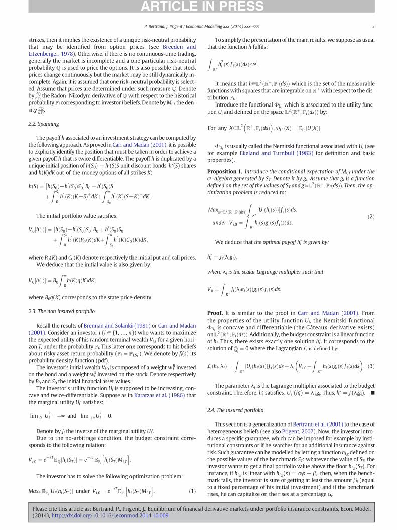
2.7.1. The CARA caseAssume that the utility function of the investor is a CRRA utility: (it

corresponds to bi = 0).

Ui xð Þ ¼ − exp −aix½ �ai

; xN0;

with ai ¼ 1τiN0, from which we deduce Ji yð Þ ¼ − ln y½ �

ai. The parameter ai

corresponds to the constant absolute risk aversion.By using the previous general results about the optimization prob-

lem, we deduce:

1) If there is no insurance constraint, the optimal payoff is given by:

h�i sð Þ ¼ Ji λigi sð Þð Þ ¼ − 1ai

ln λið Þ þ ln ψið Þ½ � þ κ i

ailn sð Þ; ð17Þ

where λi is the Lagrange parameter linked to the budget constraint.Substituting the Lagrange parameter, we get:

h�i sð Þ ¼ Vi;0erT þ κ i

ailn sð Þ−

Z ∞

0ln sð Þψis

−κ i f sð Þds �

: ð18Þ

2) If the insurance constraint is required then the optimal payoff mustbe the solution of:

MaxhiEℙi− exp −aihi STð Þ½ �

ai

�

Vi;0 ¼ e−rTEℚihi STð Þ½ �;

hi STð Þ≥hi;g STð Þ:

ð19Þ

Then, we deduce that the optimal payoff with guarantee is given by:

h��i ¼ Max hi;g ; h�i

� �; ð20Þ

where hi∗ is given in Relation (17) for an adequate initial investment

Ṽi,0.

Thus, we face two main cases:

1) μi b r. In that case, the Sharpe type ratio κi is negative, which impliesthat the optimal payoff is decreasing with respect to the risky asset.

7 As mentioned in Carr and Madan (2001), Cass and Stiglitz (1970) have proved that anecessary condition to get the two-fundmonetary separation is that investors have linearrisk tolerance. See also Gollier (2001) for more details about the choice of the utilityfunction.


2) μi N r. In that case, the Sharpe type ratio κi is positive, which impliesthat the optimal payoff is increasing with respect to the risky asset.

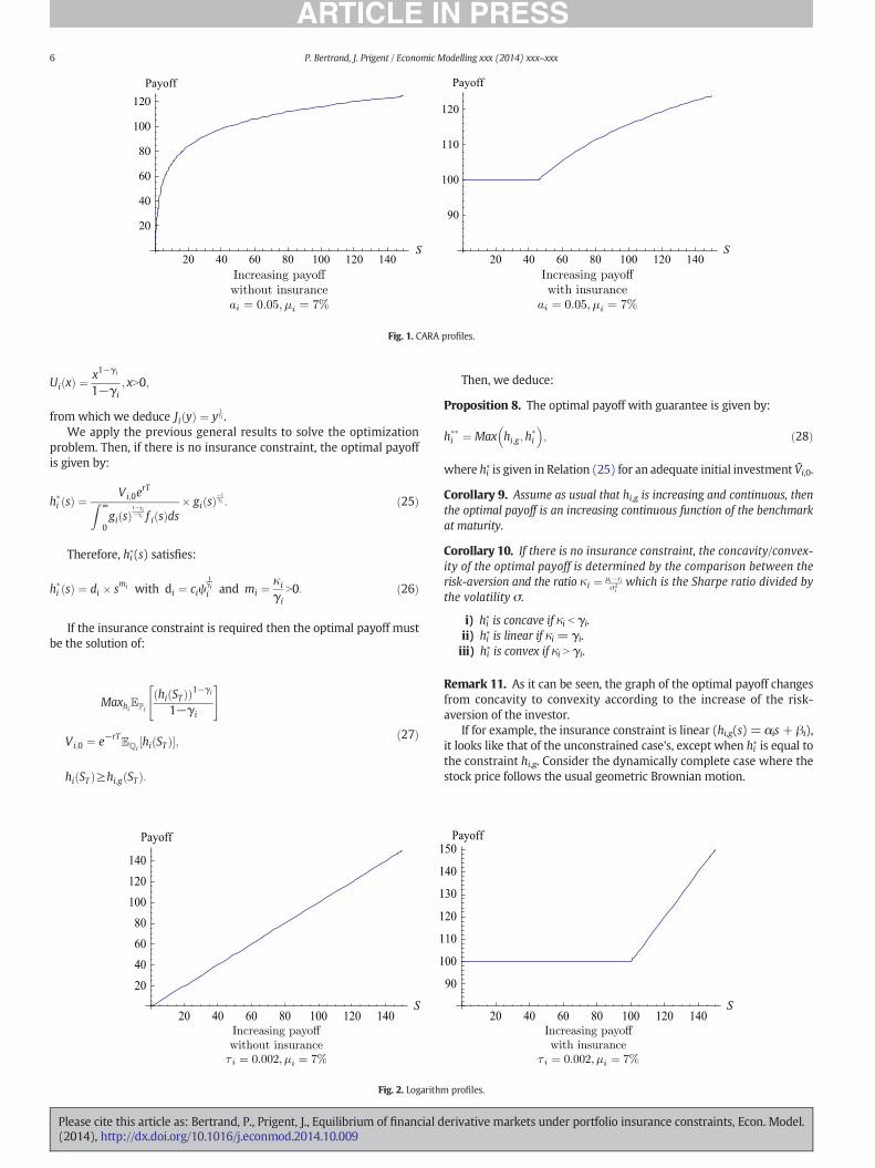
Usually, we have μi N r, as illustrated by (Fig. 1).

2.7.2. The logarithm caseAssume that the utility function of the investor is a logarithmic

utility: (it corresponds to bi = 1)

Ui xð Þ ¼ ln τi þ x½ �; xN−ai;

with τi N 0, from which we deduce Ji yð Þ ¼ 1y−τi.

The previous general results yield to the following result:

1) If there is no insurance constraint, the optimal payoff is given by:

h�i sð Þ ¼ 1λigi sð Þ−τi ¼

1λiψi

sκ i−τi; ð21Þ

where λi is the Lagrange parameter linked to the budget constraint.8

Substituting the Lagrange parameter, we get:

h�i sð Þ ¼ Vi;0erT þ τi

� � 1ψi

sκ i−τi: ð22Þ

2) If the insurance constraint is required then the optimal payoff mustbe the solution of:

MaxhiEℙiln τi þ hi STð Þ½ �½ �



ð23Þ

Then, we deduce that the optimal payoff with guarantee is given by:

h��i ¼ Max hi;g ; h�i

� �; ð24Þ

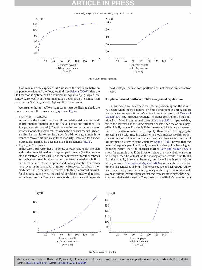
where hi∗ is given in Relation (25) for an adequate initial investmentṼi,0.The optimal payoff is concave or convex according to conditionsκi b 1 or κi N 1 (Fig. 2 and Fig. 3).

2.7.3. The HARA case

2.7.3.1. The HARA case without additional guarantee constraint. Assumethat the utility function of the investor is a HARA utility: (it correspondsto bi ≠ 0 and bi ≠ 1)

Ui xð Þ ¼ x−x̂ið Þ1−γi

1−γi; xNx̂i;

with γi ¼ 1biand x̂i ¼ − τi

bi. We deduce: Ji yð Þ ¼ x̂i þ y

1γi . The relative risk

aversion is given by:

−xU}i xð ÞU0

i xð Þ ¼ γix

x−x̂ið Þ :

If x̂i ¼ 0, the relative risk aversion is equal to the inverse of the risktolerance: γi ¼ 1

bi:

2.7.3.2. The CRRA case with an additional guarantee constraint. Assumethat the utility function of the investor is a CRRA utility. This corre-sponds to previous HARA case but with x̂i ¼ 0:

8 Note that in that case, it would be more convenient to restrict the set of all possiblesvalues of the risky asset.



20 40 60 80 100 120 140S

20

40

60

80

100

120

Payoff

20 40 60 80 100 120 140S

90

100

110

120

Payoff

Fig. 1. CARA profiles.


Ui xð Þ ¼ x1−γi

1−γi; xN0;

from which we deduce Ji yð Þ ¼ y1γi .

We apply the previous general results to solve the optimizationproblem. Then, if there is no insurance constraint, the optimal payoffis given by:

h�i sð Þ ¼ Vi;0erTZ ∞

0gi sð Þ

1−γi−γi f i sð Þds

� gi sð Þ−1γi : ð25Þ

Therefore, hi∗(s) satisfies:

h�i sð Þ ¼ di � smi with di ¼ ciψ1γii and mi ¼

κ i

γiN0: ð26Þ

If the insurance constraint is required then the optimal payoff mustbe the solution of:

MaxhiEℙi

hi STð Þð Þ1−γi

1−γi

" #



ð27Þ

20 40 60 80 100 120 140S

20406080100120140

Payoff

1

1

1

1

1

1

Fig. 2. Logarith


Then, we deduce:

Proposition 8. The optimal payoff with guarantee is given by:

h��i ¼ Max hi;g ;h�i

� �; ð28Þ

where hi∗ is given in Relation (25) for an adequate initial investment Ṽi,0.

Corollary 9. Assume as usual that hi,g is increasing and continuous, thenthe optimal payoff is an increasing continuous function of the benchmarkat maturity.

Corollary 10. If there is no insurance constraint, the concavity/convex-ity of the optimal payoff is determined by the comparison between therisk-aversion and the ratio κ i ¼ μ i−ri

σ2iwhich is the Sharpe ratio divided by

the volatility σ.

i) hi∗ is concave if κi b γi.

ii) hi∗ is linear if κi = γi.

iii) hi∗ is convex if κi N γi.

Remark 11. As it can be seen, the graph of the optimal payoff changesfrom concavity to convexity according to the increase of the risk-aversion of the investor.

If for example, the insurance constraint is linear (hi,g(s) = αis+ βi),it looks like that of the unconstrained case's, except when hi

∗ is equal tothe constraint hi,g. Consider the dynamically complete case where thestock price follows the usual geometric Brownian motion.

20 40 60 80 100 120 140S

90

00

10

20

30

40

50Payoff

m profiles.



20 40 60 80 100 120 140S

20

40

60

80

100

120Payoff

20 40 60 80 100 120 140S

90

100

110

120

130Payoff

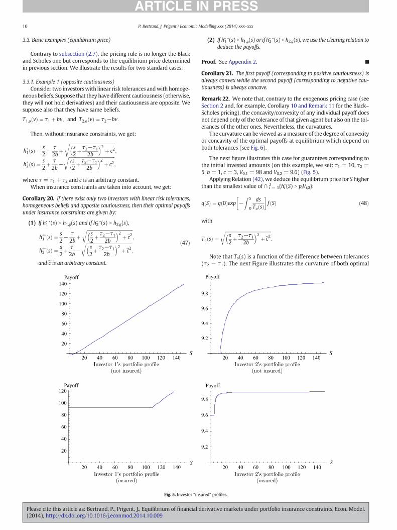
Fig. 3. CRRA concave profiles.


If we maximize the expected CRRA utility of the difference betweenthe portfolio value and the floor, we find (see Prigent (2007)) that theCPPI method is optimal with a multiple mi equal to

μ i−rσ2

i

1γi: Again, the

concavity/convexity of the optimal payoff depends on the comparisonbetween the Sharpe type ratio μ i−r

σ2iand the risk aversion.

We assume that μi N r. Two main cases must be distinguished: theconcave case and the convex case (Fig. 3 and Fig. 4).

- If κi b γi, hi∗ ∗ is concave.In this case, the investor has a significant relative risk aversion and/or the financial market does not have a good performance (itsSharpe type ratio is weak). Therefore, a rather conservative investorsearches for not too small returnswhen the financial market is bear-ish. But, he has also to require a specific additional guarantee if hewants to recover his initial capital at maturity. However, for a mod-erate bullish market, he does not make high benefits (Fig. 3).

- If κi N γi, hi∗ ∗ is convex.In that case, the investor has amoderate orweak relative risk aversionand/or the financial market has a good performance (its Sharpe typeratio is relatively high). Thus, a rather aggressive investor searchesfor the highest possible returns when the financial market is bullish.But, he has also to require a specific additional guarantee if he wantsto recover his initial capital at maturity. However, for a bearish ormoderate bullish market, he receives only this guaranteed amount.For the special case κi= γi, the optimal portfolio is linear with respectto the benchmark S. This case corresponds to the standard buy-and-

20 40 60 80 100 120 140S

50

100

150

Payoff

Fig. 4. CRRA con


hold strategy. The investor's portfolio does not involve any derivativeasset.

3. Optimal insured portfolio profiles in a general equilibrium

In this section,we determine the optimal positioning and the securi-ty design when the risk-neutral pricing is endogenous and based onmarket clearing conditions. We extend previous results of Carr andMadan (2001) by introducing general insurance constraints on the indi-vidual portfolios. In the seminal paper of Leland (1980), it is proved that,when the investor has the same market's beliefs, then the optimal pay-off is globally convex if and only if the investor's risk tolerance increaseswith his portfolio value more rapidly than when the aggregateinvestor's risk tolerance increases with global market wealth. Underthe assumption of linear risk tolerance with identical cautiousness andlog-normal beliefs with same volatility, Leland (1980) proves that theinvestor's optimal payoff is globally convex if and only if he has a higherexpected return than the financial market. Carr and Madan (2001)show for example that, if the investor thinks that the volatility is goingto be high, then he will sell at-the-money options while, if he thinksthat the volatility is going to be small, then he will purchase out-of-themoney options. Benninga and Mayshar (2000) examine the demand foroptions in a general equilibrium frameworkby agents havingHARAutilityfunctions. They prove that heterogeneity in the degree of relative riskaversion among investors implies that the representative agent has a de-creasing relative risk aversion. They show that the Black–Scholes formula

20 40 60 80 100 120 140S

90

100

110

120

130

140

Payoff

vex profiles.




does no longer hold and that all options are overpricedwith respect to theBlack–Scholes prices. Franke et al. (1998) prove also that background riskcan potentially explain option demand rather than heterogeneity inpreferences.

In what follows, we determine the optimal payoffs given the utilityfunctions, the insurance constraints, the bond and asset prices and theprobability beliefs. However, the option prices are determined endoge-nously. The agents must trade so that in particular they exchange theirderivatives position. This is the option market clearing position.

Consequently, we have the two followingmarket clearing conditions:

Xni¼1

Vi;0 ¼ S0 þ B0 andXni¼1

hi Sð Þ ¼ αSþ βB; ð29Þ

which implies that∑n

i¼1h0i Sð Þ ¼ α and zero-net supply on the option mar-

kets. Parameters α and β correspond respectively to the shares of thestock market S and the bond market B. As in Carr and Madan (2001),we can set for simplicity: α= 1 and β= 1.9

From individual expected utility maximization, we can derive thegeneral financial equilibrium properties in this static economy.

3.1. The equilibrium risk-neutral probability

The optimal positioning of a given investor is mainly based on the at-tributes of this agent. The influence of the other investors is summarizedby the risk-neutral density that takes account of their preferences and be-liefs. In what follows, we consider an economy inwhich several investorsoptimize simultaneously their respective portfolio profiles. The optionprices are no longer taken as given. It implies that the risk-neutral densityq(.) must be determined endogenously and equal to all individual pricesπi.10 This latter one must satisfy the bond pricing condition:

B0

Z þ∞

0q sð Þds ¼ B0; ð30Þ

which is equivalent to:Z þ∞

0q sð Þds ¼ 1 q :ð Þ is a pdfð Þ:

We suppose as in Carr andMadan (2001) that bonds and options arein zero net supply. Thus, in the aggregate, only the stock is held:

Xni¼1

hi STð Þ ¼ ST : ð31Þ

The previous conditions imply that the risk-neutral expected returnon the stock is equal to the riskless rate. Indeed, since each investor isendowed with δi shares with∑i = 1

n δi = 1 and that V0,i = δiS0, we de-duce that:∑i = 1

n V0,i = S0.Using budget conditions, we get:Z þ∞

0B0

Xni¼1

hi sð Þq sð Þds ¼ S0;

from which we conclude that:

B0

Z þ∞

0sq sð Þds ¼ S0 no−arbitrage conditionð Þ: ð32Þ

9 However, when dealing with a contract between specific agents such as a financial in-stitution (“the banker”) andhis customer (“the investor”), we can impose for instance thatthe initial stock position is null. Indeed the assumption α= β=1 supposes implicitly thatwe involve all financial institutions together with their clients.10 Recall that the risk-neutral density is equal to:

πi sð Þ ¼ gi sð Þ f i sð Þ;

where fi(.) is the pdf of the risky asset value ST under the statistical probability ℙ and thatgi(.) is the pdf of the Radon–Nikodym density of the risk-neutral probability.


We take S0 as given and search for the risk-neutral probability den-sity q(.), the bondprice and the optimal portfolio payoffs. In order to de-termine the risk-neutral probability density at equilibrium, recall thatthe optimal portfolio profiles with insurance constraints are given by:

h��i sð Þ ¼ hi;g sð Þ þMax h�i sð Þ−hi;g sð Þ;0h i

; ð33Þ

where hi,g denotes the guaranteed payoff and hi∗(s) corresponds to the

optimal payoff without insurance constraint (butwith amodified initialwealth). From Relation (8), the payoff hi∗(s) is given by:

dds

h�i sð Þ� � ¼ Ti;o h�i sð Þ� dds

lnf i sð Þq sð Þ �

: ð34Þ

Thus, assuming that the guaranteed payoff hi,g is differentiable,11 thederivative of the optimal payoffwith insurance constraint exists12 and isgiven by:

dds

h��i sð Þ� � ¼ dds

hi;g sð Þh i

if h�i sð Þbhi;g sð Þ; ð35Þ

and ð36Þ

dds

h��i sð Þ� � ¼ Ti;o h�i sð Þ� dds

ln1

gi sð Þ �

if h�i sð ÞNhi;g sð Þ: ð37Þ

Therefore, summing over i, we get:

Xni¼1

dds

h��i� �

sð Þ

¼Xni¼1

Ti;o h�i sð Þ� dds

ln f i sð Þ½ �− dds

ln q sð Þ½ � �

I h�i sð ÞNhi;g sð Þf g þ dds

hi;g sð Þh i

I h�i sð Þbhi;g sð Þf g:

Consequently, since ∑n

i¼1

dds

h��i� �

sð Þ ¼ 1, we get:

dds

ln q sð Þ½ �

¼−1þ

Xni¼1

Ti;o h�i sð Þ� ddsln f i sð Þ½ �

h iI h�i sð ÞNhi;g sð Þf g þ d

ds hi;g sð Þh i

I h�i sð Þbhi;g sð Þf gXni¼1

Ti;o h�i sð Þ� I h�i sð ÞNhi;g sð Þf g

;

ð38Þ

if ∑n

i¼1Ti;o h�i sð Þ�

I h�i sð ÞNhi;g sð Þf g is not null.

Solving Eq. (38), we deduce:

Proposition 12. The risk-neutral density q is given by:

For any S∈∪ni¼1 h�i Sð ÞNhi;g Sð Þn o

; q Sð Þ ¼ q 0ð Þexp −ZS0

dsT sð Þ

24 35�exp

ZS0

Xni¼1

Ti;o h�i sð Þð ÞT sð Þ

f 0i sð Þf i sð Þ �

I h�i sð ÞNhi;g sð Þf g þ h0i;g sð ÞT sð Þ I h�i sð Þbhi;g sð Þf g

!ds

24 35ð39Þ

11 For the standard case, its derivative is null since it is constant.12 There exists only a finite set of values es at which hi

∗ ∗ is non differentiable. It corre-sponds to the case: h�i esð Þ ¼ hi;g esð Þ. Generally, there exists only one such pointes. However,under usual assumptions on the existence of a pdf for the risky asset, this point has a nullprobability, so that hi∗ ∗(.) is differentiable almost everywhere with respect to ST.




where T(.) is the total risk tolerance for all payoffs higher than the re-spective guarantees of all investors, that is:

T sð Þ ¼Xni¼1

Ti;o h�i sð Þ� I h�i sð ÞNhi;g sð Þf g: ð40Þ

Corollary 13. When there does not exist any (exogenous) insurance con-straint, we get the Carr and Madan (2001) formula:

q Sð Þ ¼ q 0ð Þexp −Z S

0

dsTo sð Þ

�exp

Z S

0

Xni¼1

Ti;o h�i sð Þð ÞTo sð Þ

f 0i sð Þf i sð Þ ds

" #; ð41Þ

where To sð Þ ¼ ∑n

i¼1Ti;o h�i sð Þ�

denotes the sum of all individual tolerances.

Additionally, for homogeneous beliefs, the risk-neutral density priceis given by:


0

dsTo sð Þ

�f sð Þ: ð42Þ

If we consider the standard guarantee case for which the insuredpayoff corresponds to a constant percentage of the initial wealth piVi,0,then we get an extension of Relation (41) to the insurance case.

Denote by Smin the smallest value of the set ∪ i = 1n {hi∗(S) N piVi,0}.

Corollary 14. If at least one of the insurance constraints is not binding(S ∈ ∪ i = 1

n {hi∗(S) N piVi,0}) we deduce:

q Sð Þ ¼ q Sminð Þexp −ZSSmin

dsT sð Þ

264375exp ZS

Smin

Xni¼1

Ti;o h�i sð Þð ÞT sð Þ

f 0i sð Þf i sð Þ �

I h�i sð ÞNpiVi;0f g� �

ds

264375:

ð43Þ
Since the tolerance is defined on optimal payoffs that depend them-
selves on the risk-neutral density q, the two previous relations do notprovide explicit expression for q.

Remark 15. Note that, Relation (40) shows that the equilibrium risk-neutral density is equal to the product of a factor corresponding to

the total risk tolerance (i.e. exp −∫S

0

dsTo sð Þ

�), and a factor reflecting the

personal beliefs (called “the market” view in Carr and Madan (2001)).Note that the first factor is a positive decreasing function of therisky asset value ST which may induce a change in the mean and addnegative skewness. Carr and Madan (2001) show that, if the pdf f(s) isLognormal and the risk tolerance is constant, then the risk-neutral den-sity q(s) no longer belongs to the family of Lognormal distributions butis skewed to the left and has fatter left tails (see Bick (1987) for consis-tency of the Black–Scholes model with a general equilibriumframework).

Remark 16. With (exogenous) insurance constraints, the risk-neutraldensity is defined on ∪ i = 1

n {hi∗(s) N hi,g(s)}.This set of risky asset values ST corresponds to the case for which at

least one of the investor payoffs is above the corresponding guaranteedlevel. Otherwise, all investors recover only their guarantee. Therefore,on ∩ i = 1

n {hi∗(s) b hi,g(s)}, due to market clearing conditions, we must

have∑n

i¼1hi;g sð Þ ¼ s:

Thus, for example for fixed guaranteed amounts corresponding tothe respective insured proportions of initial wealths, we must assume

that ∑n

i¼1hi STð Þ ¼ ST þ BT : It means that the bond clearing condition

must be relaxed. Otherwise, one of the investors j must have a payoff

such that hj;g sð Þ ¼ s− ∑n

i¼1;≠ jhi;g sð Þ, but such payoff does not generally


correspond to a true guarantee. Agent j bears the risk induced by theother investors.

Note also that if one agent j has no specific guarantee (i.e. hj,g(s)=−∞) then∪ i = 1

n {hi∗(s) N hi,g(s)}=ℝ+. This latter case can correspond toa financial institution which provides its customers with guaranteedstructured products. Thus, Relation (39) allows defining the risk-neutral density q for all risky asset values.

Remark17. To compare the risk-neutral densities for the non-insuranceand insurance cases, we note that on the domain ∩ i = 1

n {hi∗(s) N hi,g(s)},the risk-neutral density has exactly the same form as in the no-insurance case.

They only differ by the levels of initial wealths. Indeed, for the insur-ance case, the initial values of the payoffs hi∗(s) are smaller than the cor-responding ones for the no-insurance case.

Thus, according to the monotonicity of the ratio Ti;o h�i sð Þð ÞTo sð Þ with respect

to the initial investment, we can deduce if for example, the risk-neutral density for the insurance case is higher or smaller than therisk-neutral density for the no-insurance case.

Note that, when the risk tolerances are constant (CARA case), theyare equal on the domain ∩ i = 1

n {hi∗(s) N hi,g(s)}, which corresponds usu-ally to rises of the risky asset.

3.2. The optimal portfolio profiles at the equilibrium

In what follows, the optimal portfolio profiles are determined fromthe financial equilibrium pricing. Contrary to the Black–Scholes pricing,the investors are now market makers.

Substituting Relation (39) with Relation (36), we deduce:

Proposition 18. The optimal portfolio profiles at the equilibrium aregiven by: If hi∗(s) b hi,g(s),

dds

h��i sð Þ� � ¼ dds

hi;g sð Þh i

;

and, if hi∗(s) N hi,g(s),

Ti;o h�i sð Þð Þ

T sð Þ þ Ti;o h�i sð Þ�

� dlnf i sð Þds

−Xnj¼1

Ti;o h�j sð Þ

� �T sð Þ

dlnf i sð Þds

Ih�j sð ÞNh j;g sð Þ � þ h0

j;g sð ÞT sð Þ I

h�j sð Þbh j;g sð Þ �0@ 1A24 35:

ð44Þ

For the non-insurance case, we recover the Carr and Madan (2001)formula:

h�i sð Þ ¼ Ti;o hi sð Þð ÞT sð Þ þ Ti;o hi sð Þð Þ � dlnf i sð Þ

ds−Xni¼1

Ti;o hi sð Þð ÞTo sð Þ

dlnf i sð Þds

!:

ð45Þ

The first term is due to the investor's risk tolerance relative to all theinvestors. The second term involves the own investor's risk toleranceand the difference between the investor's belief and a risk tolerancewhich is the weighted average of the beliefs of other investors in the fi-nancial market.

Consider now the case of homogeneous beliefs ( fi(s)= f(s)).We get:

Corollary 19. For homogeneous beliefs, we get: For hi∗(s) N hi,g(s),

dds

h��i sð Þ� � ¼ Ti;o hi sð Þð ÞT sð Þ : ð46Þ




3.3. Basic examples (equilibrium price)

Contrary to subsection (2.7), the pricing rule is no longer the Blackand Scholes one but corresponds to the equilibrium price determinedin previous section. We illustrate the results for two standard cases.

3.3.1. Example 1 (opposite cautiousness)Consider two investorswith linear risk tolerances andwith homoge-

neous beliefs. Suppose that they have different cautiousness (otherwise,they will not hold derivatives) and their cautiousness are opposite. Wesuppose also that they have same beliefs.

T1;o vð Þ ¼ τ1 þ bv; and T2;o vð Þ ¼ τ2−bv:

Then, without insurance constraints, we get:

h�1 sð Þ ¼ s2− τ

2bþ

ffiffiffiffiffiffiffiffiffiffiffiffiffiffiffiffiffiffiffiffiffiffiffiffiffiffiffiffiffiffiffiffiffiffiffiffiffiffiffiffiffiffis2þ τ2−τ1

2b

� �2 þ c2r

;

h�2 sð Þ ¼ s2þ τ2b

−ffiffiffiffiffiffiffiffiffiffiffiffiffiffiffiffiffiffiffiffiffiffiffiffiffiffiffiffiffiffiffiffiffiffiffiffiffiffiffiffiffiffis2þ τ2−τ1

2b

� �2 þ c2r

;

where τ = τ1 + τ2 and c is an arbitrary constant.When insurance constraints are taken into account, we get:

Corollary 20. If there exist only two investors with linear risk tolerances,homogeneous beliefs and opposite cautiousness, then their optimal payoffsunder insurance constraints are given by:

(1) If h1∗ ∗(s) N h1,g(s) and if h2

∗ ∗(s) N h2,g(s),

h��1 sð Þ ¼ s2− τ

2bþ


2b

� �2 þ ec2r;

h��2 sð Þ ¼ s2þ τ2b


2b

� �2 þ ec2r;

ð47Þ

and ec is an arbitrary constant.

20 40 60 80 100 120 140S

20

40

60

80

100

120

140Payoff

20 40 60 80 100 120 140S

20

40

60

80

100

120Payoff

Fig. 5. Investor “ins


(2) If h1∗ ∗(s) b h1,g(s) or if h2∗ ∗(s) b h2,g(s),we use the clearing relation to

deduce the payoffs.

Proof. See Appendix 2. ■

Corollary 21. The first payoff (corresponding to positive cautiousness) isalways convex while the second payoff (corresponding to negative cau-tiousness) is always concave.

Remark 22. We note that, contrary to the exogenous pricing case (seeSection 2 and, for example, Corollary 10 and Remark 11 for the Black–Scholes pricing), the concavity/convexity of any individual payoff doesnot depend only of the tolerance of that given agent but also on the tol-erances of the other ones. Nevertheless, the curvatures.

The curvature can be viewed as ameasure of the degree of convexityor concavity of the optimal payoffs at equilibrium which depend onboth tolerances (see Fig. 6).

The next figure illustrates this case for guarantees corresponding tothe initial invested amounts (on this example, we set: τ1 = 10, τ2 =5, b = 1, c = 3, V0,1 = 98 and V0,2 = 9.6) (Fig. 5).

Applying Relation (42), we deduce the equilibrium price for S higherthan the smallest value of ∩ i = 1

2 {hi∗(S) N piVi,0}:


0

dsTo sð Þ

�f Sð Þ ð48Þ

with

To sð Þ ¼ffiffiffiffiffiffiffiffiffiffiffiffiffiffiffiffiffiffiffiffiffiffiffiffiffiffiffiffiffiffiffiffiffiffiffiffiffiffiffiffiffiffis2þ τ2−τ1

2b

� �2 þ ec2r:

Note that To(s) is a function of the difference between tolerances(τ2 − τ1). The next Figure illustrates the curvature of both optimal

20 40 60 80 100 120 140S

9.2

9.4

9.6

9.8

Payoff

20 40 60 80 100 120 140S

9.2

9.4

9.6

9.8

Payoff

ured” profiles.



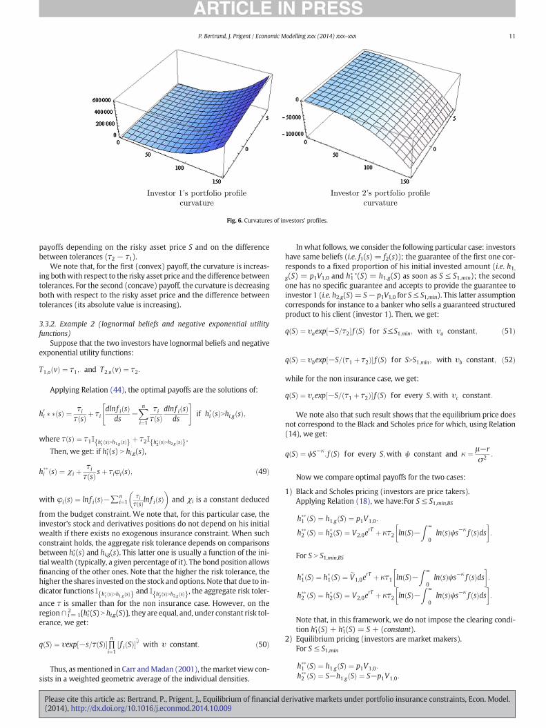
Fig. 6. Curvatures of investors' profiles.


payoffs depending on the risky asset price S and on the differencebetween tolerances (τ2 − τ1).

We note that, for the first (convex) payoff, the curvature is increas-ing bothwith respect to the risky asset price and the difference betweentolerances. For the second (concave) payoff, the curvature is decreasingboth with respect to the risky asset price and the difference betweentolerances (its absolute value is increasing).

3.3.2. Example 2 (lognormal beliefs and negative exponential utilityfunctions)

Suppose that the two investors have lognormal beliefs and negativeexponential utility functions:

T1;o vð Þ ¼ τ1; and T2;o vð Þ ¼ τ2:

Applying Relation (44), the optimal payoffs are the solutions of:

h0i � � sð Þ ¼ τiτ sð Þ þ τi

dlnf i sð Þds

−Xni¼1

τiτ sð Þ

dlnf i sð Þds

" #if h�i sð ÞNhi;g sð Þ;

where τ sð Þ ¼ τ1I h�1 sð ÞNh1;g sð Þf g þ τ2I h�2 sð ÞNh2;g sð Þf g.Then, we get: if hi∗(s) N hi,g(s),

h��i sð Þ ¼ χi þτiτ sð Þ sþ τiφi sð Þ; ð49Þ

with φi sð Þ ¼ lnf i sð Þ−∑ni¼1

τiτ sð Þlnf i sð Þ� �

and χi is a constant deduced

from the budget constraint. We note that, for this particular case, theinvestor's stock and derivatives positions do not depend on his initialwealth if there exists no exogenous insurance constraint. When suchconstraint holds, the aggregate risk tolerance depends on comparisonsbetween hi

∗(s) and hi,g(s). This latter one is usually a function of the ini-tialwealth (typically, a given percentage of it). The bondposition allowsfinancing of the other ones. Note that the higher the risk tolerance, thehigher the shares invested on the stock and options. Note that due to in-dicator functions I h�1 sð ÞNh1;g sð Þf g and I h�2 sð ÞNh2;g sð Þf g, the aggregate risk toler-

ance τ is smaller than for the non insurance case. However, on theregion∩ i=1

2 {hi∗(S) N hi,g(S)}, they are equal, and, under constant risk tol-erance, we get:

q Sð Þ ¼ υexp −s=τ Sð Þ½ �∏n

i¼1f i Sð Þ½ �

τiτ with υ constant: ð50Þ

Thus, asmentioned in Carr andMadan (2001), themarket view con-sists in a weighted geometric average of the individual densities.


In what follows, we consider the following particular case: investorshave same beliefs (i.e. f1(s) = f2(s)); the guarantee of the first one cor-responds to a fixed proportion of his initial invested amount (i.e. h1,g(S) = p1V1,0 and h1

∗ ∗(S) = h1,g(S) as soon as S ≤ S1,min); the secondone has no specific guarantee and accepts to provide the guarantee toinvestor 1 (i.e. h2,g(S)= S− p1V1,0 for S≤ S1,min). This latter assumptioncorresponds for instance to a banker who sells a guaranteed structuredproduct to his client (investor 1). Then, we get:

q Sð Þ ¼ υaexp −S=τ2½ � f Sð Þ for S≤S1;min; with υa constant; ð51Þ

q Sð Þ ¼ υbexp −S= τ1 þ τ2ð Þ½ � f Sð Þ for SNS1;min; with υb constant; ð52Þ

while for the non insurance case, we get:

q Sð Þ ¼ υcexp −S= τ1 þ τ2ð Þ½ � f Sð Þ for every S;with υc constant:

We note also that such result shows that the equilibrium price doesnot correspond to the Black and Scholes price for which, using Relation(14), we get:

q Sð Þ ¼ ψS−κ: f Sð Þ for every S;with ψ constant and κ ¼ μ−r

σ2 :

Now we compare optimal payoffs for the two cases:

1) Black and Scholes pricing (investors are price takers).Applying Relation (18), we have:For S ≤ S1,min,BS

h��1 Sð Þ ¼ h1;g Sð Þ ¼ p1V1;0:

h��2 Sð Þ ¼ h�2 Sð Þ ¼ V2;0erT þ κτ2 ln Sð Þ−

Z ∞

0ln sð Þψs−κ f sð Þds

�:

For S N S1,min,BS

h�1 Sð Þ ¼ h�1 Sð Þ ¼ eV1;0erT þ κτ1 ln Sð Þ−

Z ∞


�:

h��2 Sð Þ ¼ h�2 Sð Þ ¼ V2;0erT þ κτ2 ln Sð Þ−

Z ∞


�:

Note that, in this framework, we do not impose the clearing condi-tion h1

∗(S) + h1∗(S) = S + (constant).

2) Equilibrium pricing (investors are market makers).For S ≤ S1,min

h��1 Sð Þ ¼ h1;g Sð Þ ¼ p1V1;0:

h��2 Sð Þ ¼ S−h1;g Sð Þ ¼ S−p1V1;0:




For S N S1,min

h��1 Sð Þ ¼ χ1 þτ1

τ1 þ τ2S; ð53Þ

h��2 Sð Þ ¼ χ2 þτ2

τ1 þ τ2S; ð54Þ

since, due to homogeneous beliefs φi(s) = 0. Thus, the optimal pay-offs are piecewise linear which is not true for the Black and Scholespricing for which they are based on logarithm function (see Fig. 1).

Remark23. Wenote that, if beliefs are homogenous and utilities exhib-it CARA, optimal payoffs are linear functions with respect to the riskyasset price. In that case, the slopes of the profiles are simply equal tothe ratios of the risk tolerance of each given investor divided by thesum of all the risk tolerances. Thus, the higher the risk tolerance, thehigher the slope. It means that the higher the risk tolerance, the higherthe exposure to the risky asset, which is quite intuitive.

4. Conclusion

Using the expected utility theory framework, we determine the op-timal payoffs and their prices at equilibrium under insurance con-straints on the horizon wealth for a large class of models. The resultsprove that derivative assets have to be introduced in the portfolio tomaximize the expected utilities of investors. The optimal solution clear-ly depends on the risk aversion of the investor and on the specificationof the guarantee at maturity. Under the standard assumptions that theinsurance constraints and the payoff are modelled by continuous func-tions of the risky asset, the solution is equal to the maximum betweenthis function and the solution of the unconstrained problem but witha different initial wealth. These optimal portfolios can be determinedfor quite general utility functions, stock prices and insurance con-straints. In the no guarantee case, the concavity/convexity of the portfo-lio profile is determined from the degree of risk aversion and from thefinancial market performance, for example a Sharpe type ratio. Thiskind of result still holds according to the insurance constraint atmaturi-ty.We show that, even with exogenous insurance constraints, the equi-librium risk-neutral density is equal to the product of a factorcorresponding to the total risk tolerance, and a factor reflecting the per-sonal beliefs, which is a generalization of Carr and Madan (2001). Notethat the first factor is a positive decreasing function of the risky assetvalue which may imply a change in the mean and involve negativeskewness.

Appendix 1. (Proof of Proposition 2 about the optimal portfolioprofile with guarantee constraint)

To solve the following optimization problem:

MaxhiEℙi½Uiðhi STð Þ�

with Vi;0 ¼ e−rTEℙihi STð ÞMi;T

h i;

and hi STð Þ≥hi;g STð Þ;ð55Þ

let us introduce the sets:

Ki;1 ¼ hi∈L2 ℝþ;ℙi dsð Þ

� ��Vi;0 ¼ e−rTEℙihi STð ÞMi;T

h in oand

Ki;2 ¼ hi∈L2 ℝþ;ℙi dsð Þ

� ��hi≥hi;0n o

:


The set Ki = Ki,1 ∩ Ki,2 is a convex set of L2(R+, Pi(ds)). Consider thefollowing indicator function of Ki, denoted by δKi

and defined by:

δKihið Þ ¼ 0 if hi∈Ki

þ∞ if hi∉Ki

�:

Since Ki is closed and convex, δKiis lower semi-continuous and

convex.Recall the notion of subdifferentiability: (see for example Ekeland

and Turnbull (1983) for definition and properties of subdifferentials).

1) Let V denote a Banach space and b.,.N the duality symbol;2) For any function H defined on Vwith values inℝ ∪ {+∞}, a continu-

ous affine functional l : V→ ℝ everywhere less than h (i.e. ∀ v ∈ V,l(v) ≤ N H(v)) is exact at v∗ ∗ if l(v∗ ∗) = H(v∗ ∗);

3) A functionH : V→ℝ∪ {+∞} is subdifferentiable at v∗ ∗ if there exists acontinuous affine functional l(.) = b., vl N− a, everywhere less thanH, which is exact at v∗ ∗. The slope vl of such an l is a subgradient of Hat v∗ ∗. The set of all subgradients ofH at v∗ is the subdifferential ofH atv∗ ∗ and is denoted by ∂H(v∗ ∗).

Recall the following characterization:

vc∈∂H v��

i f f H v��

bþ ∞ and ∀v∈V ; bv−v��; vcNþ H v��

≤H vð Þ:ð56Þ

Denote by ∂δK the subdifferential of δK. The optimization problem isequivalent to:

Maxh E½Uðh XTð Þ�−δK hð Þð Þ: ð57Þ

The optimality conditions leads to the following result:There exists a scalar λc and a function hc defined on L2 ℝþ;ℙ dsð Þð Þ

such that:

h�� ¼ J λcg þ hcð Þ; ð58Þ

where λc is the solution of the following problem: Find y such that

V0 ¼Z ∞

0J yg sð Þ þ hc sð Þ½ �g sð Þ f sð Þds

and hc∈∂δK2h��ð Þ.

Proof. Denote by ℒ the functional defined by

ℒ hð Þ ¼ −E U h STð Þð Þ½ � þ δK hð Þð Þ:

The optimization problem

Maxh E½Uðh STð Þ�−δK hð Þð Þ ð59Þ

is equivalent to the following:

−Minh ℒ hð Þð Þ; ð60Þ

where ℒ is subdifferentiable and h∗ ∗ is a solution of the optimal problem if0 ∈ ∂L(h∗ ∗).ΦU is continuous and, due to the kind of constraints, δK is contin-uous. Thus:

∂ℒ ¼ ∂ −ΦU þ δKð Þ ¼ ∂ −ΦUð Þ þ ∂ δKð Þ:




Moreover, sinceΦU is differentiable then ∂(ΦU)= {ΦU′}. Additionally,we have:

∂ δKð Þ ¼ ∂ δK1

� �þ ∂ δK2

� �:

From the characterization (56), h1∈∂δK1 h��ð Þ if and only if

∀h;Z ∞

0h−h��

sð Þh1 sð Þℙ dsð Þ þ δK1h��

≤δK1hð Þ:

In particular, ∀ h ∈ K1, ∫0∞ (h − h∗ ∗)(s)h1(s)ℙ(ds) ≤ 0, from which

we deduce that h1 is orthogonal to any orthogonal function to the sub-space generated by g. Thus, there exists a scalar λc such that h1 = λcg.

To conclude, 0 ∈ ∂L(h∗ ∗) if there exists hc∈∂δK2 h��ð Þ such that

0 ¼ −U0 h�� þ λcg þ hc: ■

To explain more precisely the condition hc∈∂δK2 h��ð Þ, assume thatthe insurance constraint h0 and hc are continuous.13 Consequently, theoptimal payoff h∗ ∗ is continuous. Recall that from the characterization(56), we deduce:

∀h∈L2 ℝþ;ℙ dsð Þ

� �;

Z ∞

0h−h��

sð Þ hcð Þ sð Þℙ dsð Þ þ δK2h��

≤δK2hð Þ:

In particular:

∀h∈L2 ℝþ;ℙ dsð Þ

� �such that h≥h0;

Z ∞

0h−h��

sð Þhc sð Þℙ dsð Þ≤0:

From the previous condition, we deduce:

- If ∀ s∈ I, h∗ ∗(s) N h0(s) then, on each compact subinterval Ico of I, wecan considermco equal to theminimumof h∗ ∗− h0 on Ico.mco is non-negative. Now, consider the function h equal to h��− mco1Icoð Þ. Byconstruction, h N h0 everywhere. Therefore, the relation ∫(h −h∗ ∗)(s)hc(s)ℙ(ds) ≤ 0 is true.

This implies that:

mco

ZIco

hc sð Þℙ dsð Þ≥0:

On the other hand, by letting h equal to h∗ + a where a is a non-negative constant, a∫

Icohc sð Þℙ dsð Þ≤0. Consequently, since for all Ico,∫Ico

hc sð Þℙ dsð Þ ¼ 0, hc is equal to 0 on the product of intervals I. Considernow for all Ico, a function h equal to h�� þ a1Ico . Then, the relation ∫(h− h∗ ∗)(s)hc(s)ℙ(ds) ≤ 0 becomes a∫

Icohc sð Þℙ dsð Þ≤0, from which the

negativity of hc on I is deduced.Therefore, we deduce the following properties:Under the above assumption, the function hc satisfies the following

property:

1) If on an I product of intervals of values of ST, h∗ ∗(ST) N h0(ST) then hc isequal to 0 on I.

2) If on an I product of intervals of values of ST, h∗ ∗(ST)= h0(ST) then hcis negative on I.

Now, from the assumptions on the marginal utility U′, we deducethat its inverse J is a continuous and decreasing function with:

limoþ J ¼ þ∞ and limþ∞ J ¼ 0:

Thus, for all s, the function λc→h�� λc; sð Þ ¼ Max h0 sð Þ; eh λc; sð Þ� �

iscontinuous and decreasing. Therefore, the function λc→Eℚ h�� λc; STð Þ½ �is continuous and decreasing from +∞ to Eℚ h0 λc; STð Þ½ � which is

13 Such properties are always verified in practice.


lower than the initial investment V0. From the intermediate values the-oremandbymonotonicity,we deduce that, under theprevious assump-tions on the utility U, there is one and only one continuous optimalpayoff, associated to the unique solution λc of the budget equation.

Appendix 2. (Optimal portfolio profiles at the equilibrium) Proof ofCorollary (20)

Recall that under homogeneous beliefs, the optimal portfolio profilessatisfy:

dds

h��i sð Þ� � ¼ h0i;g sð Þ if h��i sð Þbhi;g sð Þ;Ti;o hi sð Þð Þ

T sð Þ ; if h��i sð ÞNhi;g sð Þ: ð61Þ

Due to the linear risk tolerance, we get:

dds

h��1 sð Þ� � ¼ h01;g sð Þ; if h��1 sð Þbh1;g sð Þ ð62Þ

dds

h��2 sð Þ� � ¼ h02;g sð Þ; if h��2 sð Þbh2;g sð Þ ð63Þ

dds

h��1 sð Þ� � ¼ τ1 þ b1h��1 sð Þ

τ þ b1h��1 sð Þ þ b2h

��2 sð Þ ; if h��1 sð ÞNh1;g sð Þ ð64Þ

dds

h��2 sð Þ� � ¼ τ2 þ b2h��2 sð Þ

τ þ b1h��1 sð Þ þ b2h

��2 sð Þ ; if h��2 sð ÞNh2;g sð Þ: ð65Þ

This system of ordinary differential equations can be explicitlysolved if the cautiousness is opposite b1 = b = − b2 (see for example,Carr and Madan, 2001). Indeed, we have:

Case 1. If h1∗ ∗(s) N h1,g(s) and h2∗ ∗(s) N h2,g(s),

h01�� sð Þ

h02�� sð Þ ¼

τ1 þ bh��1 sð Þτ2−bh��2 sð Þ :

Substituting h1∗ ∗(s) = s − h2

∗ ∗(s) leads to a quadratic equation forh2∗ ∗(s):

12

h��2 sð Þ� �2− s2þ τ2b

h ih��2 sð Þ þ τ2sþ η

2b¼ 0;

with solution:


−ffiffiffiffiffiffiffiffiffiffiffiffiffiffiffiffiffiffiffiffiffiffiffiffiffiffiffiffiffiffiffiffiffiffiffiffiffiffiffiffiffiffis2þ τ2b

h i2− τ2sþ η

2b

r;

from which we deduce:

h�1 sð Þ ¼ s2− τ

2bþ

ffiffiffiffiffiffiffiffiffiffiffiffiffiffiffiffiffiffiffiffiffiffiffiffiffiffiffiffiffiffiffiffiffiffiffiffiffiffiffiffiffiffis2þ τ2b

h i2− τ2sþ η

2b

r:

We must set η≤ τ1τ2b . Then, let ec be defined from equation:

η ¼ τ1τ2b

−ec2b:We finally deduce that the optimal payoffs are given by:

h��1 sð Þ ¼ s2− τ

2bþ


2b

� �2 þ ec2r;



2b

� �2 þ ec2r:

ð66Þ




Case 2. If h1∗ ∗(s) b h1,g(s) and h2∗ ∗(s) b h2,g(s),

h��1 sð Þ ¼ h1;g sð Þ;h��2 sð Þ ¼ h2;g sð Þ: ð67Þ

Case 3. If h1∗ ∗(s) N h1,g(s) and h2∗ ∗(s) b h2,g(s),

h��1 sð Þ ¼ s−h2;g sð Þ;h��2 sð Þ ¼ h2;g sð Þ: ð68Þ

Case 4. If h1∗ ∗(s) b h1,g(s) and h2∗ ∗(s) N h2,g(s),

h��1 sð Þ ¼ h1;g sð Þ;h��2 sð Þ ¼ s−h1;g sð Þ: ð69Þ

References

Arditti, F., John, K., 1980. Spanning the state space with options. J. Financ. Quant. Anal. 15,1–9.

Bazak, S., 1995. A general equilibrium model of portfolio insurance. Rev. Financ. Stud. 8,1059–1090.

Bazak, S., Shapiro, A., 2001. Value-at-risk based risk management: optimal policies andasset prices. Rev. Financ. Stud. 14, 371–405.

Benninga, S., Mayshar, J., 2000. Heterogeneity and option pricing. Rev. Deriv. Res. 40,1341–1352.

Bertrand, P., Lesne, J.-P., Prigent, J.-L., 2001. Gestion de portefeuille avec garantie:l'allocation optimale en actifs dérivés. Finance 22, 7–35.

Bertrand, P., Prigent, J.-L., 2010. A note on risk aversion, prudence and portfolio insurance.Geneva Risk Insur. Rev. 35, 81–92.

Bick, A., 1987. On the consistency of the Black–Scholes model with a general equilibriumframework. J. Financ. Quant. Anal. 22, 259–276.

Black, F., Perold, A.R., 1992. Theory of constant proportion portfolio insurance. J. Econ.Dyn. Control 16, 403–426.

Black, F., Jones, R., 1987. Simplying portfolio insurance. J. of Portfolio Manag 48–51 (Fall1987).

Brennan, M.J., Schwartz, R., 1989. Portfolio insurance and financial market equilibrium. J.Bus. 62, 455–472.

Brennan, M.J., Solanki, R., 1981. Optimal portfolio insurance. J. Financ. Quant. Anal. 16 (3),279–300.

Brady, N., et al., 1988. Report of the Presidential Task Force on Market Mechanisms. U.S.Government Printing Office, Washington D.C.

Breeden, D., Litzenberger, R., 1978. Prices of state contingent claims implicit in optionsprices. J. Bus. 51, 621–651.

Carr, P., Madan, D., 2001. Optimal positioning in derivative securities. Quant. Financ. 1,19–37.


Cass, D., Stiglitz, J., 1970. The structure of investor preferences and asset returns and sep-arability in portfolio allocation. J. Econ. Theory 2, 122–160.

Cox, J., Huang, C.-F., 1989. Optimal consumption and portfolio policies when assets pricesfollow a diffusion process. J. Econ. Theory 49, 33–83.

Cvitanic, J., Karatzas, I., 1996. Contingent claim valuation and hedging with constrainedportfolio. In: Davis, M., Duffie, D., Fleming, W., Shreve, S. (Eds.), IMA Volume inMath 65, pp. 13–33.

Das, S., 2000. Structured Products and Hybrid Securities, 2nd ed. John Wiley and Sons,New York, NY.

Driessen, J., Maenhout, P., 2007. An empirical portfolio perspective on option pricinganomalies. Eur. Finan. Rev. 11, 561–603.

Duffie, D., Jackson, M., 1989. Optimal innovation of futures contracts. Rev. Financ. Stud. 2,275–296.

Eeckhoudt, L., Gollier, C., 2005. The impact of prudence on optimal prevention. EconomicTheory 26, 989–994.

Ekeland, I., Turnbull, T., 1983. Infinite-dimensional optimization and convexity. ChicagoLectures in Mathematics. the University of Chicago Press.

El Karoui, N., Jeanblanc, M., Lacoste, V., 2005. Optimal portfolio management withAmerican capital guarantee. J. Econ. Dyn. Control 29, 449–468.

Franke, G., Stapleton, R., Subrahmanyam, M., 1998. Who buys and who sells options: therole of options in an economy with background risk. J. Econ. Theory 82, 89–109.

Friesen, P., 1979. The Arrow Debreu model extended to financial markets. Econometrica47, 689–707.

Gollier, 2001. The Economics of Risk and Time. MIT Press.Grossman, S., Vila, J.L., 1989. Portfolio insurance in complete markets: a note. J. Bus. 60,

275–298.Grossman, S., Zhou, J., 1996. Equilibrium analysis of portfolio insurance. J. Financ. 51,

1379–1403.Hakansson, N., 1978. Welfare aspects of options and supershares. J. Financ. 33, 759–776.Hens, T., Riger, M.O., 2008. The dark side of the moon: structured products from the

customer's perspective. Working Paper 459. ISB, Université de Zurich.Johnston, L., McConnell, J., 1989. Requiem for a market: an analysis of the rise and fall of a

financial futures contract. Rev. Financ. Stud. 2, 1–24.Karatzas, I., Lehoczky, J., Sethi, S.P., Shreve, S.E., 1986. Explicit solution of a general con-

sumption/investment problem. Math. Oper. Res. 11, 261–294.Kreps, D., 1982. Multiperiod Securities and the Efficient Allocation of Risk: A Comment on

the Black–Scholes Option Pricing Model. University of Chicago Press, Chicago, IL, pp.203–232 (Chapter 6).

Leland, H., 1980. Who should buy portfolio insurance? J. Financ. 35, 581–594.Leland, H.E., Rubinstein, M., 1976. The evolution of portfolio insurance. In: Luskin, D.L.

(Ed.), Portfolio Insurance: A Guide to Dynamic Hedging. Wiley.Perold, A. (1986). Constant portfolio insurance. Harvard Business School. Unpublished

manuscript.Perold, A., Sharpe, W., 1988. Dynamic strategies for asset allocation. Financial Analyst

Journal, pp. 16–27, (January–February).Prigent, J.-L., 2007. Portfolio Optimization and Performance Analysis. Chapman & Hall,

Boca Raton, Florida.Ross, S., 1976. Options and efficiency. Quant. J. Econ. 90, 75–89.Stoimenov, P.A., Wilkens, S., 2005. Are structured products “fairly” priced? An analysis of

the German market for equity-linked instruments. J. Bank. Financ. 29, 2971–2993.Tversky, A., Kahneman, D., 1992. Advances in prospect theory: cumulative representation

of uncertainty. J. Risk Uncertain. 5, 297–323.


http://refhub.elsevier.com/S0264-9993(14)00364-2/rf0005















































































Documents

Equilibrium of financial derivative markets under portfolio insurance constraints