Equilibrium Directed Search with Multiple

Applications∗

James Albrecht

Department of Economics

Georgetown University

Washington, D.C. 20057

Pieter A. Gautier

Free University Amsterdam

Tinbergen Institute

Susan Vroman

Department of Economics

Georgetown University

Washington, D.C. 20057

January 30, 2006

1 Introduction

In this paper, we construct an equilibrium model of directed search in a largelabor market in which unemployed workers make multiple job applications.Specifically, we consider a matching process in which job seekers, observingthe wages posted at all vacancies, send their applications to the vacanciesthat they find most attractive. At the same time, each vacancy, when itchooses its wage posting, takes into account that its posted wage influencesthe number of applicants it can expect to attract. We assume that eachunemployed worker makes a fixed number of applications, a. Each vacancy(among those receiving applications) then chooses one applicant to whom itoffers its job. When a > 1, there is a possibility that more than one vacancywants to hire the same worker. In this case, we assume that the vacancies inquestion can compete for this worker’s services. The introduction of multipleapplications adds realism to the directed search model, and, in addition, af-fects the efficiency properties of equilibrium. In the benchmark competitive

∗

We thank the anonymous referees and our editor, Fabrizio Zilibotti, for detailed and

helpful comments. We also thank Ken Burdett, Behzad Diba, Benoit Julien, Vladimir

Karamychev, Ian King, Harald Lang, Dale Mortensen, Lucas Navarro, and Rob Shimer.

1

search equilibrium model (Moen 1997), equilibrium is constrained efficient.We show that changing the basic directed search model to allow workers tomake more than one application results in equilibria that are not constrainedefficient. This means there is a role for labor market policy in the directedsearch framework.

When a = 1, our model is essentially the limiting version of Burdett, Shi,and Wright (2001) (hereafter BSW) translated to a labor market setting.BSW derive a unique symmetric equilibrium in which (in the labor marketversion) all vacancies post a wage between zero (the monopsony wage) andone (the competitive wage). The value of this common posted wage dependson the number of unemployed, u, and the number of vacancies, v, in themarket. Letting u, v →∞ with v/u = θ, the equilibrium posted wage is anincreasing function of θ. BSW do not consider normative questions. Moen’sresult is that in a large labor market, directed search implements whathe calls competitive search equilibrium. Competitive search equilibriumis constrained efficient in the following sense. Assume there is a cost pervacancy created. A social planner would choose a level of vacancy creation— or, in a large labor market, a level of labor market tightness, θ, — to tradeoff the cost of vacancy creation against the benefit of making it easier forworkers to match. Moen shows that the θ the social planner would chooseis the same as the one that arises in competitive search equilibrium. Usinga different approach, we also show that equilibrium in a directed searchmodel is constrained efficient in a large labor market when a = 1. Moreimportantly, however, we show that if each worker makes a finite numberof multiple applications, that is, if a ∈ {2, ...,A}, where A is any arbitrary,finite integer, then equilibrium in a directed search model is not constrainedefficient. Specifically, too many vacancies are posted (θ is too high) in free-entry equilibrium relative to the constrained efficient level. Equivalently,vacancies pay the workers who take their jobs too low a wage on average.

Our model is also related to Julien, Kennes, and King (2000) (hereafterJKK). JKK assume that each unemployed worker posts a minimum wageat which he or she is willing to work, i.e., a “reserve wage,” and that eachvacancy, observing all posted reserve wages, then makes an offer to oneworker. If more than one vacancy wants to hire the same worker, then, asin our model, there is ex post competition for that worker’s services. Thisis equivalent to a model in which each worker applies to every vacancy, i.e.,a = v, sending the same reserve wage in each application. Each vacancythen chooses one worker at random to whom it offers a job. If a workerhas more than one offer, then there is competition for his or her services.In a finite labor market, JKK show that the unique, symmetric equilibrium

2

reserve wage lies between the monopsony and competitive levels. There isthus equilibrium wage dispersion in their model. Those workers who receiveonly one offer are employed at the reserve wage, while those who receivemultiple offers are employed at the competitive wage. In the limiting labormarket version of JKK, the symmetric equilibrium reserve wage convergesto zero, and free-entry equilibrium is again constrained efficient.

In our model, when a ∈ {2, ...,A}, all vacancies post the monopsony wagein the unique symmetric equilibrium. As in JKK, this leads to equilibriumwage dispersion. Some workers (those who receive exactly one offer) areemployed at the monopsony wage, and some workers (those who receivemultiple offers) have their wages bid up to the competitive level. The keydifference between our model and both BSW and JKK, however, is thatfree-entry equilibrium is inefficient. When a ∈ {2, ...,A}, there is excessivevacancy creation.

The inefficiency arises because when a ∈ {2, ...,A}, two coordinationfrictions operate simultaneously. The first is the well-known urn-ball friction;some vacancies receive no applications while others receive more than one.In addition, a new friction is introduced by multiple applications. Someworkers receive multiple offers while others receive none. As a result, somevacancies with applicants fail to hire a worker. In BSW, only the urn-ballfriction is present; in JKK, only the multiple-application friction applies.The market cannot correct both frictions at the same time. In our model,competition among vacancies, once applications have been made, can solvethe multiple-application friction. This leads, however, to a posted wage thatis too low to correct the urn-ball friction and that consequently generatestoo many vacancies.

The outline of the rest of the paper is as follows. In the next section, wederive our basic positive results in a single-period framework. Specifically,treating θ as given, we derive the matching function and the symmetricequilibrium posted wage. In Section 3, we endogenize θ by allowing for freeentry of vacancies. This lets us compare the free-entry equilibrium levelof θ to the constrained efficient level (the two values of θ are the samewhen a = 1, different when a ∈ {2, ...,A}, and the same once again asa → ∞). In Section 4, we present a steady-state version of our model forthe case of a ∈ {2, .., A}. The key to the steady-state analysis is that aworker who receives only one offer in the current period has the option toreject that offer in favor of waiting for a future period in which more than onevacancy bids for his or her services. This leads to a tractable model in whichlabor market tightness and the equilibrium wage distribution are determinedsimultaneously. The normative results that we derived in the single-period

3

model continue to hold in the steady-state setting. In Section 5, we considerthree extensions. Specifically, (i) we allow workers to choose how manyapplications to make, (ii) we relax the assumption that each vacancy canconsider only one worker’s application, and (iii) we allow vacancies to followstrategies that rule out Bertrand competition. These extensions, while ofinterest in their own right, also serve as robustness checks — our basic resultthat the free-entry equilibrium value of θ is constrained inefficient whena ∈ {2, ...,A} continues to hold. Finally, we conclude in Section 6.

2 The Basic Model

We consider a game played by u homogeneous unemployed workers and (theowners of) v homogeneous vacancies. This game has several stages:

1. Each vacancy posts a wage.

2. Each unemployed worker observes all posted wages and then submitsa applications with no more than one application going to any onevacancy.

3. Each vacancy that receives at least 1 application randomly selects oneto process. Any excess applications are returned as rejections.

4. A vacancy with a processed application offers the applicant the postedwage. If more than one vacancy makes an offer to a particular worker,then each vacancy can increase its bid for that worker’s services.

5. A worker with one offer can accept or reject that offer. A worker withmore than one offer can accept one of the offers or reject all of them.

Workers who fail to match with a vacancy and vacancies that fail to matchwith a worker receive payoffs of zero. The payoff for a worker who matcheswith a vacancy is w, where w is the wage that he or she is paid. A vacancythat hires a worker at a wage of w receives a payoff of 1−w. This is a modelof directed search in the sense that workers observe all wage postings anddirect their applications to vacancies with attractive wages and/or whererelatively little competition is expected. We assume that vacancies cannotpay less than their posted wages.

Before we analyze this game, some comments on the underlying assump-tions are in order. First, we are treating a as a parameter of the searchtechnology; that is, the number of applications is taken as given. In general,

4

a ∈ {1, 2, ..., A}. Second, we assume that it takes a period for a vacancy toprocess an application. This is why vacancies return excess applications asrejections. This processing-time assumption captures the idea that whenworkers apply for several jobs at the same time, firms can waste time andeffort pursuing applicants who ultimately go elsewhere. Finally, we assumethat a vacancy that faces competition for its selected applicant always hasthe option to increase its offer. This means that workers who receive morethan one offer have their wages bid up via Bertrand competition to w = 1,the competitive wage.1 In Section 5, we consider the implications of relaxingeach of these assumptions. We show that endogenizing a, allowing vacan-cies to process more than one application, and allowing vacancies that arecompeting for an applicant to pursue a different tie-breaking strategy do notreverse our main results.

We consider symmetric equilibria in which all vacancies post the samewage and all workers use the same mixed strategy to direct their applica-tions.2 We do not consider equilibria in which workers follow asymmetricapplication strategies since this would require unrealistic implicit coordina-tion. We do our analysis in a large labor market in which we let u, v →∞with v/u = θ keeping a ∈ {1, 2, ...,A} fixed. We show that for each (θ, a)combination there is a unique symmetric equilibrium, and we derive the cor-responding equilibrium matching probability and posted wage. Assuming(for the moment) the existence of a symmetric equilibrium, we begin withthe matching probability.

1One might think of ruling out ex post bidding by assumption, but then there wouldbe no common equilibrium posted wage. To see this, suppose all vacancies post a wageof w. Then, assuming that a worker who has multiple offers accepts the highest one, itis in the interest of any vacancy to post a slightly higher wage so long as w is not tooclose to one. The reason is that if a vacancy posts a wage ε above the common wage, itsprobability of hiring a worker jumps discontinuously since it “wins” whenver the workerhas multiple ofers. Once w is sufficiently close to one, a vacancy can profit by lowering itswage to the minimum level consistent with attracting one or more applicants with somepositive probability. This is similar to the argument given in Burdett and Judd (1983) fornonexistence of a single-price equilibrium.

2One could alternatively consider symmetric equilibria in which vacancies follow mixedstrategies, so that more than one wage is posted in equilibrium. This approach is taken inGalenianos and Kircher (2005), which combines elements of our paper and that of Chadeand Smith (2004). In Galenianos and Kircher (2005), a vacancy whose chosen applicanthas other offer(s) is precluded by assumption from increasing its initial offer, even thoughit would be in its interest to do so, given that other vacancies have committed to notchanging their offers. The assumption that vacancies cannot engage in ex post biddingis restrictive, but without it, equilibrium in Galenianos and Kircher (2005) would not besubgame perfect.

5

LetM(u, v; a) be the expected number of matches in a labor market with

u unemployed workers and v vacancies when each unemployed worker sub-

mits a applications. Then m(θ;a) = limu,v→∞,v/u=θ

M(u, v; a)

uis the matching

probability for an unemployed worker in a large labor market.

Proposition 1 Let u, v → ∞ with v/u = θ and a ∈ {1, ...,A} fixed. The

probability that a worker finds a job converges to

m(θ;a) = 1− (1−θ

a(1− e−a/θ))a. (1)

The proof is given in Albrecht et. al. (2004); see also Philip (2003).In Appendix A, we sketch the idea of the proof to clarify the relationshipbetween our matching probability and the finite-market matching functionspresented in BSW (the standard urn-ball matching function) and JKK (theurn-ball matching function with the roles of u and v reversed).

For use below, we note the following properties of m(θ;a):(i) m(θ;a) is increasing and concave in θ,

limθ→0

m(θ;a) = 0, and limθ→∞

m(θ;a) = 1;

(ii)m(θ; a)

θis decreasing in θ, 3

limθ→0

m(θ;a)

θ= 1, and lim

θ→∞

m(θ;a)

θ= 0.

The effect of a on m(θ; a) is less clearcut. Treating a as a continuous

variable, we find that ma(θ; a) ≷ 0 asa

1− q

∂q

∂a− ln(1 − q) ≷ 0 where

q =θ

a(1 − e−a/θ) is the probability that any one application leads to an

offer. For moderately large values of θ (θ > 1

2, approximately), m(θ; a)

first increases and then decreases with a. This nonmonotonicity reflects thedouble coordination problem that arises when workers apply to more thanone but not all vacancies. The first coordination problem is the standardone associated with urn-ball matching, namely, that some vacancies canreceive applications from more than one worker, while others receive none.

3 Interestingly,m(θ; a)

θis not convex in θ, as can be seen immediately by considering

the case of a = 1. The properties of m(θ; a) andm(θ; a)

θgiven in (i) and (ii) are the

minimal ones required for our normative results in Sections 3 and 4 below.

6

With multiple applications, there is a second coordination problem, this

time among vacancies. When workers apply for more than one job at a

time, some workers can receive offers from more than one vacancy, while

others receive none. Ultimately, a worker can only take one job, and the

vacancies that “lose the race” for a worker will have wasted time and effort

while considering his or her application. The matching function derived

in BSW captures only the urn-ball friction, while the one derived in JKK

captures only the multiple-application friction. Our matching probability

incorporates both these frictions, and the interaction between these two

frictions provides new insights.

Proposition 1 and its implications are only interesting if a symmetric

equilibrium exists. We now turn to the existence question.

Proposition 2 Consider a large labor market in which u, v → ∞ with

v/u = θ. There is a unique symmetric equilibrium to the wage-posting game.

When a = 1, all vacancies post a wage of

w(θ; 1) =1

θe−1/θ

(1− e−1/θ). (2)

When a ∈ {2, ...,A}, all vacancies post a wage of w(θ; a) = 0, and the

fraction of wages paid that are equal to one is

γ(θ;a) =1− (1− θ

a(1− e−a/θ))a − θ(1− e−a/θ)(1− θa(1− e−a/θ))a−1

1− (1− θa(1− e−a/θ))a

.

(3)

The proof is given in Appendix B. The basic idea is as follows. Toprove the existence of a symmetric equilibrium, we show that w(θ; 1) hasthe property that if all vacancies, with the possible exception of a “potentialdeviant,” post that wage, then it is also in the interest of the deviant topost that wage. When a ∈ {2, ...,A}, however, no matter what the commonwage posted by other vacancies, it is always in the interest of the deviant toundercut that common wage. This forces the wage down to the monopsonylevel, which in our single-period model is w = 0.

The equilibrium wage for the case of a = 1 is equal to one minus theprice given in Proposition 3 in BSW — again with the appropriate notationalchange. The tradeoff that leads to a well-behaved equilibrium wage, w ∈(0, 1), when a = 1 is the standard one in equilibrium search theory. To seethis, note that the profit for a deviant (D) from offering w′ rather than thecommon posted wage, w, can be written as:

π(w′;w) = (1−w′)P [D gets at least one application]P [selected applicant has no other offer],

7

where the third term equals 1 when a = 1. As any particular vacancyincreases its posted wage, holding the wages posted at other vacancies con-stant, the profit that this vacancy generates conditional on attracting anapplicant, (1 − w′), decreases. At the same time, however, the probabil-ity that it attracts at least one applicant increases. This tradeoff variessmoothly with θ; so the equilibrium wage varies smoothly between zero andone. Thus, as emphasized in BSW (p. 1069), there is a sense in whichfrictions “smooth” the operation of the labor market.

When a ∈ {2, ...,A}, the posted wage collapses to the monopsony level(as in Diamond (1971)). The intuition for this result is based on the changein the tradeoff underlying equilibrium wage determination. This change —to be described below — has two implications. First, the equilibrium wage islower than when a = 1. Second, when a ∈ {2, ...,A}, the lower is the putativecommon equilibrium wage w, the stronger is the incentive to deviate byposting w′ < w. This second implication is what drives the wage down tothe monopsony level.

Why is the equilibrium wage lower when workers make more than oneapplication? Note first that the incentive to deviate from a common postedwage w comes from the first two terms in π(w′;w) since the third term isunaffected by changes in w′ when the labor market is large. That is, theincentive to deviate comes from the effect of w′ on 1−w′ and on the proba-bility that the deviant receives at least one application. The effect of offeringw′ on 1 − w′ is obviously the same whether workers make one or multipleapplications. However, a deviation has less effect on the probability thatthe deviant gets at least one applicant when workers make multiple appli-cations. Consider a deviation w′ > w. The higher wage makes the vacancymore attractive to a worker if w′ is the only offer received. However, whena ∈ {2, ..., A}, workers have an interest in getting multiple offers in orderto generate Bertrand competition for their services, and since the deviantvacancy is more attractive to all workers, applying to the deviant decreasesthe probability that this occurs. Thus, a deviation w′ > w increases theprobability that the deviant receives at least one application by less whenworkers make multiple applications than when a = 1. Similarly, a deviationw′ < w decreases the probability that the deviant receives at least one ap-plication by less than when a = 1. In this case, a worker who applies to thedeviant gets a lower wage if this is the only offer received. Just as whena = 1, this makes the deviant less attractive. However, when a ∈ {2, ...,A},to increase the chance of getting multiple offers, workers have an incentiveto apply to a “safe” job where others are less likely to apply. Relative to thecase of a = 1, this reduces the decrease in the probability that the deviant

8

attracts at least one applicant. The fact that upward deviations are lessattractive and downward deviations are more attractive explains why theequilibrium wage is lower when a ∈ {2, ...,A} than when a = 1.

Why does the equilibrium wage fall to the monopsony level when workersmake multiple applications? The potential benefit to a deviant of postinga wage that is ε below a common wage w is the same for all w, but thecost in terms of the reduction in the probability of receiving at least oneapplication falls as the common wage falls. The probability that the deviantreceives at least one application depends on the chance that workers arewilling to take to try to generate multiple offers. The closer w is to zero,the greater is the benefit to a worker of receiving multiple offers; i.e., thegreater is the difference between the competitive wage and w. Thus, theincentive for workers to apply to a vacancy offering ε below the commonwage, w, rises as w falls, and the probability that a vacancy offering ε lessthan w receives at least one application rises as w falls. Thus, as w falls,the potential benefit of a downward deviation is constant, but the cost ofsuch a deviation decreases. This is what drives the common wage to themonopsony level.

Interestingly, when a ∈ {2, ...,A}, the equilibrium outcome in our di-rected search model is the same as the outcome one would find in a randomsearch model in which workers make multiple applications and vacanciesengage in Bertrand competition when their candidates have multiple offers.If workers do not observe posted wages, they apply at random to a va-cancies in symmetric equilibrium, and the matching rate is the same as inour model. In addition, vacancies pay the monopsony wage in this randomsearch model, unless a worker has multiple offers, in which case Bertrandcompetition drives the wage to the competitive level. Thus, allowing formultiple applications in our model erases the difference between directedand random search in terms of outcomes in contrast to the case of a = 1.To the best of our knowledge, no random search model with multiple appli-cations and Bertrand competition exists in the literature, but it would bestraightforward to construct such a model. Postel-Vinay and Robin (2002) isthe most closely related model. In their model, wage offers arrive at Poissonrates to both the unemployed and the employed. If a worker who is alreadyemployed receives another offer, then that worker’s current employer andprospective new employer engage in Bertrand competition for his or her ser-vices. In the homogeneous worker/homogeneous firm version of their model,this leads to a two-point distribution of wages paid, namely, the monopsonywage and the competitive wage, as in our model.

9

Finally, despite the fact that the posted equilibrium wage in our modelis zero when a ∈ {2, ..., A}, there is still a sense in which “the wage” variessmoothly with θ. The expected fraction of wages paid that are equal to one,γ(θ;a), has the following properties:(i) γ(θ; a) is increasing in θ and in a;(ii) lim

θ→0

γ(θ; a) = 0 and limθ→∞

γ(θ; a) = 1.

The fact that γ is increasing in θ is exactly as one would expect — as thelabor market gets tighter, the chance that an individual worker gets multipleoffers increases. To understand why γ is also increasing in a, it is importantto remember that γ(θ;a) is the expected wage for those workers who matchwith a vacancy; in particular, those workers who fail to match are not treatedas receiving a wage of zero. Finally, defining γ(θ) = lim

a→∞γ(θ; a), we can show

γ(θ) =1− e−θ − θe−θ

1− e−θ. (4)

This is the expected wage in a large labor market when each worker sendsout an arbitrarily large number of applications.

3 Efficiency

We now turn to the question of constrained efficiency. The result suggestedby the efficiency of competitive search equilibrium holds in our setting whena = 1; however, when workers make a fixed number of multiple applications,this result breaks down.

Suppose vacancies are set up at the beginning of the period and that eachvacancy is created at cost cv. The efficient level of labor market tightness4

is determined as the solution to

maxθ≥0

m(θ;a)− cvθ.

The first-order condition for this maximization is

cv =mθ(θ∗; a). (5)

4 In a finite labor market with u given, the social planner chooses v to maximize

M (u, v; a) − cv, i.e., expected output (equal to the expected number of matches sinceeach match produces an output of 1) minus the vacancy creation costs. Dividing themaximand by u and letting u, v →∞ with v/u = θ gives the maximand in the text.

10

The equilibrium level of labor market tightness is determined by free entry.

When a = 1, this means

cv =m(θ∗∗; 1)

θ∗∗(1−w(θ∗∗; 1)), (6)

whereas for a ∈ {2, ...,A}, the condition is

cv =m(θ∗∗; a)

θ∗∗(1− γ(θ∗∗; a)). (7)

Equations (6) and (7) reflect the condition that entry (vacancy creation)occurs up to the point that the cost of vacancy creation is just offset bythe value of owning a vacancy. This value equals the probability of hiringa worker times the expected surplus generated by a hire — equal to 1 minusthe posted wage when a = 1 and to 1 minus the expected wage when a ∈{2, ..., A}.

Note that θ∗ denotes the constrained efficient level of labor market tight-ness and θ∗∗ denotes the equilibrium level of labor market tightness. At issueis the relationship between θ∗ and θ∗∗.

Proposition 3 Let u, v → ∞ with v/u = θ and a ∈ {1, ...,A} fixed. For

a = 1, θ∗ = θ∗∗. For a ∈ {2, ..., A}, θ∗∗ > θ∗.

Proof. Differentiating equation (1) with respect to θ gives

mθ(θ; a) = (1−θ

a(1− e−a/θ))a−1(1− e−a/θ −

a

θe−a/θ). (8)

For the case of a = 1, substituting this into equation (5) gives an implicitexpression for θ∗,

cv = 1− e−1/θ∗

−

1

θ∗e−1/θ

∗

.

Using equations (1) and (2) in equation (6) gives an implicit expression forθ∗∗,

m(θ∗∗; 1)

θ∗∗(1−w(θ∗∗; 1)) = 1− e−1/θ

∗∗

−

1

θ∗∗e−1/θ

∗∗

.

Thus, equations (5) and (6) imply θ∗ = θ∗∗ when a = 1.When a ∈ {2, ...,A}, substituting equation (8) into equation (5) implies

that θ∗ solves

cv = (1−θ∗

a(1− e−a/θ

∗

))a−1(1− e−a/θ∗

−a

θ∗e−a/θ

∗

), (9)

11

whereas, using equations (1) and (3), θ∗∗ (equation (7)) solves

cv = (1−θ∗∗

a(1− e−a/θ

∗∗

))a−1(1− e−a/θ∗∗

). (10)

The right-hand sides of both (9) and (10) are decreasing in θ. Since theright-hand side of (10) is greater than that of (9) for all θ > 0, it followsthat θ∗∗ > θ∗.

Posting a vacancy has the standard congestion and thick-market effectsin our model — adding one more vacancy makes it more difficult for the in-cumbent vacancies to find workers but makes it easier for the unemployed togenerate offers. A striking result of the competitive search equilibrium lit-erature is that adding one more vacancy causes the wage to adjust in such away as to balance these external effects correctly. One way to interpret thisresult is that competition leads to a wage that satisfies the Hosios (1990)condition in a Nash bargaining model. Equivalently, one can say (Moen,1997, p. 387) that the competitive search equilibrium wage has the prop-erty that the marginal rate of substitution between labor market tightnessand the wage is the same for vacancies as for workers. The first part ofProposition 3 shows that this result holds when one uses an explicit urn-ball(a = 1) microfoundation for the matching function. When workers makemultiple applications, however, the result that θ∗∗ > θ∗ indicates that theequilibrium level of vacancy creation is too high. Equivalently, the equilib-rium expected wage is below the level that would be indicated by the Hosioscondition.

A first intuition for why we find constrained efficiency with a = 1 but notwith a fixed, finite number of multiple applications is that with a = 1, onlyone coordination problem affects the operation of the labor market, whereaswith a fixed a ∈ {2, ..., A}, the urn-ball and the multiple-applications coor-dination problems operate simultaneously. Adding a vacancy increases thenumber of matches by reducing the first coordination friction, the one thatworkers impose on each other, but at the same time increases the second co-ordination friction, the one that vacancies impose on each other. When eachworker applies to only one vacancy, the second friction is absent, but withmultiple applications there are two coordination problems that cannot besolved simultaneously. This intuition does not, however, address the ques-tion of why there is too much vacancy creation, as opposed to not enough.Accordingly, we now give a more detailed explanation of our inefficiencyresult.

The social planner opens vacancies as long as the marginal social benefitexceeds cv, while the market opens vacancies as long as the marginal (=

12

average) private benefit exceeds cv. When a = 1, the private benefit of a newvacancy equals the social benefit. When a ∈ {2, ..., A}, the private benefitexceeds the social benefit. The social benefit of a new vacancy is simply

mθ(θ;a); the private benefit ism(θ;a)

θ(1−γ(θ;a)). The key to understanding

the discrepancy between the private and social benefits of a new vacancywhen a ∈ {2, ...,A} is to note that mθ(θ;a) can be expressed as

mθ(θ; a) =m(θ;a)

θ(1− γ(θ;a))p(θ; a). (11)

where

• m(θ;a)/θ is the probability that a vacancy receives at least one appli-cation

• 1−γ(θ;a) is the probability that the worker who has been offered thejob has no other offers

• p(θ;a) =1− e−a/θ − a

θe−a/θ

1− e−a/θis the probability that a vacancy receives

two or more applications conditional on receiving at least one.

One can derive equation (11) by differentiating m(θ;a), but this ex-pression can also be derived using a straightforward economic argument. Avacancy has value to the social planner if it leads to an otherwise idle worker

being employed and producing output. With probabilitym(θ; a)

θ, a vacancy

is filled and produces one unit of output. However, with probability γ(θ;a),the worker who matches with the vacancy also receives another offer. In thiscase, the social benefit of the vacancy is zero; if it had not been opened, thenumber of matches would have been the same. The private benefit in thiscase is also zero — a vacancy receives nothing if it makes its offer to a workerwho has other offer(s) since the wage is bid up to the competitive level.Social and private incentives are thus aligned with respect to the first twoterms on the right-hand side of equation (11). The social planner considersan additional factor, which is given by p(θ;a). Consider the creation of anew vacancy. If p(θ;a) = 0, then all vacancies have at most one applicant.Opening a new vacancy creates no social benefit because any applicant thatit might attract would leave another vacancy unfilled. On the other hand, ifp(θ;a) = 1, a new vacancy, if it is filled, does not leave another vacancy withno applicants. In general, the lower is p(θ;a), the more likely it is that a new

13

vacancy will cause an incumbent vacancy to fail to attract any applicantsand hence the lower the social benefit.

To further understand our inefficiency result, we ask what wage, w∗,should have been posted in the first stage of the game in order to achieveefficiency? In other words, if the social planner could only determine thewage and not θ, what wage would she post? The efficient wage has to satisfy

mθ(θ; a) =m(θ;a)

θ(1− γ(θ;a))(1−w∗);

that is,

w∗(θ; a) = 1− p(θ;a) =aθe−(a/θ)

1− e−(a/θ).

When a = 1, w∗ equals the posted wage given in equation (2) in Proposition2. The fact that the posted wage is zero when a ∈ {2, ..., A} is what leads toan inefficient outcome. The inefficiency problem when workers make multi-ple applications could thus be solved by an appropriately chosen minimumwage.

According to the Hosios condition, efficiency requires that the expectedprivate benefit of opening a vacancy equals the marginal contribution ofthat vacancy to the matching process and that the expected wage equals theworker’s marginal contribution to the matching process. The efficient wagew∗ equals the probability that a vacancy receives exactly one applicationconditional on receiving at least one. This conditional probability is themarginal contribution of a worker to the matching process because outputis only increased if the worker applies to a vacancy with no other applicants.When workers apply to more than one vacancy and there is ex post Bertrandcompetition among vacancies, workers apply to vacancies even if they post azero wage, and vacancies receive more surplus than their contribution to thematching process warrants. This is why there is excessive vacancy creationin equilibrium.

It is interesting to note that the equilibrium outcome is again Paretoefficient when we let a→∞. To see this, note that

m(θ) = lima→∞

m(θ;a) = 1− e−θ

and

γ(θ) = lima→∞

γ(θ;a) =1− e−θ − θe−θ

1− e−θ

and substitute these into the efficiency and equilibrium conditions as inthe proof of Proposition 3. Alternatively, following the route suggested by

14

equation (11), note that as a→∞, p(θ; a)→ 1, thus aligning the social andprivate benefits of vacancy creation.5 This result is Proposition 2.5 in JKK.

In a companion paper, Julien, Kennes, and King (2006) show that equi-librium in a finite labor market with a = v is also constrained efficient ifone assumes a particular wage determination mechanism; namely, vacanciesoffering jobs to workers who have no other offers receive all of the surplus(w = 0) but vacancies offering jobs to workers who do have other offers re-ceive none of the surplus (w = 1). Julien, Kennes, and King (2006) interpretthis result in terms of what they call the Mortensen rule (Mortensen 1982)— that efficiency in matching is attained if the “initiator” of the match getsthe total surplus. By mimicking our proof of Proposition 2, we can showthat this assumed wage determination mechanism is in fact the symmetricequilibrium outcome in a directed search model with wage posting whena = v in a finite labor market.6

Could an adaptation of the Julien, Kennes, and King (2006) wage deter-mination mechanism to a large labor market with a ∈ {2, ..., A} deliver theconstrained efficient outcome? In order to do this, we would have to assumethat a worker receives w = 1 if he or she (i) has multiple offers or (ii) hasonly one offer and is the only applicant to the vacancy making that offer butreceives w = 0 if he or she has only one offer but the vacancy making thatoffer has other applicants. The extra twist in the mechanism (setting w = 1in case (ii) above) is required because p(θ; a) < 1 when a �= v. This mecha-nism delivers an expected payoff to vacancy creation equal to the right-handside of equation (11); thus, it implements the constrained efficient outcome.

We argue, however, that this wage determination protocol cannot besustained as an equilibrium outcome in a large labor market. One reasonis that it requires that when a worker is the sole applicant for a job, thevacancy has to reveal this, even though it is not in the vacancy’s interest to

5The fact that the social planner cannot improve on the equilibrium outcome in this

case does not mean that welfare increases as a → ∞. To the contrary, γ(θ; a) increases

and m(θ; a) decreases in a as a → ∞. Increasing a makes the planner’s problem more

difficult. Similarly, even though equilibrium is constrained efficient when a = 1, welfaremay increase by moving to a > 1.

6The intuition for constrained efficiency in a large labor market when a = 1 is quite

different from the intuition for the finite labor market case when a = v. In the former,

constrained efficiency is a result of competition, and competition requires a labor market

sufficiently large that individual vacancies have negligible market power. When a = v,

constrained efficiency is a result of perfect monopoly power — the entire surplus goes to

the vacancy if there is no competition for the applicant it selects and to the worker if he

or she winds up having the monopoly power. The monopoly intuition does not require

that the labor market be large.

15

do so. More fundamentally, even if a worker somehow knew that he or she

was the only candidate for a job, this wage determination protocol would not

survive if one allowed for competing mechanisms. The proposed mechanism

gives an applicant an expected payoff of

γ(θ;a) + (1− γ(θ; a))(1− p(θ;a)) = γ(θ;a) + (1− γ(θ; a))w∗(θ;a).7

Note, however, that the proposed mechanism is equivalent in terms of ex-pected payoff to one in which each vacancy posts w∗(θ; a) and pays thatwage to its selected applicant unless that applicant has multiple offers, inwhich case the wage is bid up to one by Bertrand competition. However,Proposition 2 tells us that the proposed mechanism is not an equilibrium.If all vacancies were “in effect” posting w∗(θ; a), it would be in the inter-est of individual vacancies to post a slightly lower wage. Although we donot want to claim that it is “impossible” to find a mechanism that couldimplement the efficient outcome, the above argument suggests that Propo-sition 3 is more general than one might suspect at first glance. Specifically,this argument rules out any alternative mechanism that (i) has full ex post

competition (and, by equation (11), full ex post competition is required forefficiency) and (ii) yields a positive expected payoff when a worker receivesonly one offer.

4 Steady State

We now turn to steady-state analysis for a labor market with directed searchand multiple applications. We work with the limiting case in which u, v →∞with v/u = θ and a ∈ {2, ..., A} fixed. Since only the ratio of v to u mattersin the limiting case, we normalize the labor force to 1; thus, u is interpretedas the unemployment rate.

In steady-state, workers flow into employment with probability m(θ; a)per period. We assume that matches break up exogenously with probabilityδ, giving the countervailing flow back into unemployment. Similarly, jobs

move from vacant to filled with probabilitym(θ; a)

θand back again with

probability δ. Steady-state analysis thus allows us to endogenize vacanciesand unemployment. More importantly, moving to the steady state means

7An applicant with multiple offers gets the full surplus (this occurs with probabilityγ(θ; a)) as does an applicant who receives only one offer but does so from a vacancy thathas no other applicants (this occurs with probability (1− γ(θ; a))(1− p(θ; a)). Otherwise,the applicant gets nothing.

16

that those unemployed who fail to find an acceptable job in the currentperiod can wait and apply again in the future. In the case of a = 1, this isnot particularly interesting since, in equilibrium, there is no gain to waiting.However, with multiple applications, the ability of the unemployed to holdout for a situation in which vacancies engage in Bertrand competition fortheir services, albeit at the cost of delay, implies a positive reservation wage.This leads to a simple and appealing model in which labor market tightnessand the reservation wage are simultaneously determined. On the one hand,the lower is the reservation wage of the unemployed, the more vacancies firmswant to create. On the other hand, as the labor market becomes tighter, i.e.,as θ increases, the unemployed respond by increasing their reservation wage.The steady-state equilibrium reservation wage is positive, thus suggestingthat moving to the steady-state might restore efficiency. Our final result inthis section shows that this is not the case — there is still excessive vacancycreation.

The analysis proceeds as follows. Suppose the unemployed set a reser-vation wage R. With multiple applications, the wage-posting problem for avacancy is qualitatively the same as in the one-period game. Whatever com-mon wage might be posted at other vacancies, each individual vacancy hasthe incentive to undercut. In the one-period game, this implies a monop-sony wage of w = 0; in the steady state, this same mechanism implies adynamic monopsony wage of w = R.8 To avoid complicated dynamics, weassume that a vacancy that fails to hire its candidate in period t cannotcarry its queue of remaining applicants (if any) over to the next period. Asa consequence, workers start with a new application round in each periodsince their earlier applications are no longer on file. This implies that theprobability that an unemployed worker finds a job in any period and theprobability that he or she is hired at the competitive wage, conditional onfinding a job, are the same as in the single-period model; i.e., equations (1)and (3) for m(θ;a) and γ(θ; a) continue to apply.

We begin by examining the value functions for jobs and for workers. Ajob can be in one of three states — vacant, filled paying the competitive wage,and filled paying R. Let V, J(1), and J(R) be the corresponding values. The

8We restrict our attention to stationary strategies (as do JKK in their dynamic exten-sion). That is, we rule out reputation mechanisms that might avert bidding wars. Sinceany two vacancies that might consider avoiding a bidding war today interact directly inany future period with probability zero, this seems reasonable. We consider a mechanismthat rules out Bertrand competition in a static setting in Section 5.3 below.

17

value of a vacancy is

V = −cv+1

1 + r{m(θ;a)

θ[γ(θ; a)J(1)+(1−γ(θ;a))J(R)]+(1−

m(θ;a)

θ)V }.

Maintaining a vacancy entails a cost cv, which is incurred at the start ofeach period. Moving to the end of the period, and thus discounting at

rate r, the vacancy has hired a worker with probabilitym(θ;a)

θ. With

probability γ(θ;a), the worker who was hired had his or her wage bid upto the competitive level, thus implying a value of J(1). With probability1 − γ(θ; a) the worker was hired at w = R, thus implying a value of J(R).

Finally, with probability 1 −m(θ;a)

θ, the vacancy failed to hire, in which

case the value V is retained.Free entry implies V = 0 so the analysis for vacancies remains the same;

that is, free entry turns the dynamic game into one that is essentially staticfor vacancies. Given V = 0, there is no incentive for vacancies competingfor a worker to drop out of the Bertrand competition before the wage isbid up to w = 1 (thus justifying the notation J(1)). This in turn impliesthat we also have J(1) = 0. Inserting these equilibrium conditions into theexpression for V gives

m(θ;a)

θ(1− γ(θ;a))J(R) = cv(1 + r).

At the same time, the value of employing a worker at w = R is

J(R) = (1−R) +1

1 + r[(1− δ)J(R) + δV ].

Again using V = 0, we have

J(R) =1 + r

r+ δ(1−R).

Combining these equations gives the first steady-state equilibrium condition,

cv =m(θ; a)

θ(1− γ(θ; a))

1−R

r + δ. (12)

A worker also passes through three states — unemployed, employed atthe competitive wage, and employed at R. The value of unemployment isdefined by

U =1

1 + r{m(θ;a)[γ(θ; a)N(1) + (1− γ(θ;a))N(R)] + (1−m(θ; a))U},

18

where N(1) and N(R) are the values of employment at w = 1 and w = R,

respectively. These latter two values are in turn defined by

N(1) = 1 +1

1 + r{(1− δ)N(1) + δU}

N(R) = R+1

1 + r{(1− δ)N(R) + δU}.

The reservation wage property, i.e., N(R) = U, then implies

U =1 + r

rR

N(1) =(1 + r)

r(r + δ)(r + δR).

Inserting these expressions into the expression for U and rearranging givesthe second steady-state equilibrium condition,

R =m(θ;a)γ(θ;a)

r + δ +m(θ; a)γ(θ;a). (13)

The final equation for the steady-state equilibrium is the standard flow(Beveridge curve) condition for unemployment. Since the labor force isnormalized to 1, this is

u =δ

δ +m(θ; a). (14)

Equations (13) and (14) show that, as is common in this class of models,once labor market tightness (θ) is determined, the other endogenous vari-ables — in this case, R and u — are easily determined. Using equation (13)to eliminate R from equation (12) gives the equation that determines thesteady-state equilibrium value of θ, namely,

cv =m(θ∗∗;a)

θ∗∗1− γ(θ∗∗; a)

r + δ +m(θ∗∗;a)γ(θ∗∗; a). (15)

Using our results on the properties of m(θ; a) and γ(θ;a), we can show that

the right-hand side of equation (15) equals1

r + δas θ → 0, that it goes to

zero as θ → ∞, and that its derivative with respect to θ is negative for all

θ > 0. Equation (15) thus has a unique solution for each cv ∈ (0,1

r + δ].

The natural next step is to compare equilibrium steady-state labor mar-ket tightness with the constrained efficient value of θ. The planner’s problem

19

is to choose the level of labor market tightness that maximizes the discountedvalue of output net of vacancy costs for an infinitely-lived economy.9 Thatis, the planner’s problem is to maximize

∞∑s=0

(1

1 + r

)s

(1− us − cvθsus)

subject tous+1 − us = δ(1− us)−m(θs;a)us

with u0 given.The Lagrangean for this problem is

∞∑s=0

(1

1 + r

)s

[(1− us − cvθsus) + λs(us+1 − us − δ(1− us) +m(θs; a)us)]

The necessary conditions for this problem evaluated at the steady state are

−cvu+ λmθ(θ; a)u = 0

−1− cvθ + λ[r + δ +m(θ; a)] = 0

Eliminating λ gives

cv =(1 + cvθ

∗)mθ(θ∗; a)

r + δ +m(θ∗;a). (16)

Now we can compare the levels of labor market tightness implied byequations (15) and (16). Using equations (1) and (3), equation (15) can berewritten as

cv(r+δ+m(θ∗∗; a)) = (1+cvθ∗∗)(1−

θ∗∗

a(1−e

−a/θ∗∗))a−1(1−e−a/θ∗∗). (17)

Using equation (8), equation (16) can be rewritten as

cv (r + δ +m(θ∗; a)) = (1+cvθ∗)(1−

θ∗

a(1−e−a/θ

∗

))a−1(1−e−a/θ∗

−

a

θ∗e−a/θ∗).

(18)As in the single-period analysis, θ∗ is the constrained efficient level of labormarket tightness, i.e., the value of θ that solves equation (16), and θ

∗∗ is theequilibrium level of labor market tightness, i.e., the value of θ that solvesequation (15). Comparing equations (17) and (18) yields the following:

9We consider only stationary solutions, but this is not likely to be restrictive in our

model. There are two standard reasons why a nonstationary solution might be optimal.First, as shown in Shimer and Smith (2001), a nonstationary solution can be optimal ina matching model with two-sided heterogeneity when agents’ characteristics are comple-ments in production. A nonstationary solution may also be optimal if there are increasingreturns to scale in the matching function. Neither of these features is present in our model.

20

Proposition 4 Let u, v → ∞ with v/u = θ and a ∈ {2, ...,A} fixed. Then

in steady state, θ∗∗ > θ∗.

Proposition 4 indicates that, as in the single-period analysis, when theunemployed make a fixed number of multiple applications per period (a ∈{2, ..., A}), equilibrium is constrained inefficient. Specifically, there is toomuch vacancy creation. This result holds even though the ability of theunemployed to reject offers in favor of waiting for a more favorable outcomein some future period implies a dynamic monopsony wage above the single-period monopsony wage of zero. The intuition for the inefficiency result isthe same as in the static model. As before, the social benefit of opening anadditional vacancy, the right-hand side of equation (18), is p(θ;a) times theprivate benefit, the right-hand side of equation (17).

5 Extensions and Robustness Checks

In this section, we focus on three simplifying assumptions that we madein our basic model. These assumptions are: (i) that the number of appli-cations sent out by each worker is a parameter of the search technology,(ii) that each vacancy can process at most one applicant per period, and(iii) that two or more vacancies competing for the same worker engage inBertrand competition for that worker’s services. Accordingly, we examinewhat happens to our results if (i) the number of applications per worker is achoice variable, (ii) each vacancy can process more than one applicant, and(iii) vacancies pursue strategies that rule out Bertrand competition. In allthree robustness exercises, we confirm our result that equilibria in modelsof directed search with multiple applications are inefficient.

5.1 Endogenous a

We have assumed that each worker makes a applications, where a ∈ {1, 2, ..., A}is exogenously given. Since the equilibrium level of labor market tightnessis efficient when a = 1 but inefficient when a ∈ {2, ...,A}, it is natural toask whether — and under what circumstances — workers would choose tomake only one application or more than one. In addressing this question,we consider only pure-strategy symmetric equilibria in application strate-gies. That is, assuming that all other workers make a applications, underwhat conditions (taking into account how firms react to all workers choosinga) is it in the individual worker’s interest also to choose a?

21

To make endogenizing a an interesting problem, there must be a costassociated with applications, so we assume that each application costs ca tosubmit. In the one-shot game, there are then only 2 exogenous parameters,the cost of posting a vacancy, cv, and the cost of submitting an application,ca. We need only consider 0 ≤ cv ≤ 1 and 0 ≤ ca ≤ 1 since worker outputequals 1 and if cv > 1, no firm would post a vacancy, and if ca > 1, noworker would make an application. Thus for each (cv, ca) in the unit squarewe can ask (i) what are the free-entry equilibrium values of θ and a and (ii)what values of θ and a would a social planner choose?

We start with the equilibrium problem and ask: For what values of(cv, ca) is a = 1 consistent with equilibrium? For what values of (cv, ca) isa = 2 consistent with equilibrium? Etc. We address this problem numeri-cally as follows.

Consider a candidate equilibrium in which all workers make a applica-tions. Then, for each θ, we know what wage vacancies choose to post (fromequation (2) if a = 1; zero if a ∈ {2, ..., A}), and we know m(θ;a). We picka value of cv from a grid over (0, 1). From the free-entry condition (equation(6) if a = 1; equation (7) otherwise), there is a corresponding implied valueof θ. We then ask, using the value of θ implied by the free-entry condition,for what values of ca is an individual worker’s expected payoff maximized bychoosing to send out the same number of applications as all other workersdo? We answer this numerically by comparing the expected payoff associatedwith choosing a when all other workers also choose a with those associatedwith choosing a − 1, a − 2, ... and a + 1, a + 2, ..., etc.10 For the particularcv that we chose, this gives us a range of values for ca. We then repeat forthe next value of cv, etc. The outcome of this algorithm is the set of (cv, ca)combinations in the unit square that are consistent with a pure-strategysymmetric equilibrium in which all workers make a applications. We carryout this process for a wide range of values for a.

Next, we address the social planner’s problem. Given (cv, ca), the naturalsocial planner’s problem is

maxθ,a

m(θ;a)− cvθ − caa,

where θ ≥ 0 and a ∈ {0, 1, 2, ...}. We know this problem is concave in θ for agiven a. Thus, if (θ∗, a∗) solves the social planner’s problem, we must have

cv =mθ(θ∗;a∗),

10This comparison can be carried out in a finite number of steps since the maximum

number of applications a worker might make is limited by the requirement that the total

cost of submitting applications be less than one.

22

and θ∗ = θ∗(a∗; cv) has a unique solution. We can plug this back intothe social planner’s objective and maximize numerically with respect to a.

This gives a∗ (and θ∗) as functions of (cv, ca). We can then compare theequilibrium unit square with the social planner unit square.

The qualitative results of this exercise are as follows. First, althoughthere are many parameter configurations for which the equilibrium numberof applications, a∗∗, equals 1, this outcome requires relatively high values ofca. Second, the equilibrium number of applications increases as ca falls (asone would expect). Third, there are parameter configurations that admitmultiple equilibria. This reflects a complementarity between workers’ andfirms’ strategies. For example, if all workers choose a = 1, then vacanciespost a positive wage, w(θ; 1) > 0. For some values of θ (equivalently, for somevalues of cv) it is not worthwhile for workers to submit a second application.On the other hand, if all workers choose a = 2, then w = 0, and it cannotbe worthwhile for a worker to deviate to a = 1. Fourth, there are manyparameter configurations for which no symmetric pure-strategy equilibriumexists. One parameter region in which this is the case is the set of (cv, ca)combinations in which individual workers would prefer not to send out anyapplications when all other workers choose a = 1. This occurs when both cvand ca are relatively high. There are, however, other (cv, ca) combinationsfor which no symmetric pure-strategy equilibrium exists. Fifth, for relativelylow values of ca, there are parameter regions with unique equilibria at a∗∗ =2, a∗∗ = 3, etc.

In the parameter regions in which a symmetric pure-strategy equilibrium(or equilibria) exists, we find a∗∗ ≥ a∗. Specifically, there are parameterconfigurations for which a∗ = a∗∗ = 1 (where a∗∗ = 1 may either be uniqueor one of two or more equilibrium possibilities). However, when a∗∗ ≥ 2,we find a∗∗ > a∗. This occurs when cv and ca are low relative to the outputproduced by a match. That is, for what we view as reasonable values of cvand ca, the equilibrium number of applications exceeds the socially optimalvalue. The reason is simply that individual workers, when deciding howmany applications to submit, fail to take into account the externality theyimpose on other workers. The countervailing effect that one might expect —that an increase in worker applications should make it easier for firms to filltheir vacancies — is not sufficient to offset this externality and, indeed, mayeven be negative because of the coordination failure among vacancies.

Finally, endogenizing a does not affect our basic result that, while di-rected search with one application always leads to the efficient level of labormarket tightness, this is not the case with multiple applications. For (cv, ca)combinations such that a∗ = a∗∗ = 1, we, of course, have θ∗ = θ∗∗. For

23

almost all parameter configurations for which a∗∗ > a∗, we find θ∗∗ > θ∗ aswe did before. There is a small set of parameter configurations, however,for which θ∗∗ < θ∗.11 This appears at first glance to be inconsistent withProposition 3, but note that in that Proposition, we imposed the restrictionthat a∗ = a∗∗.

The bottom line of this robustness exercise is that when a is endoge-nous and when workers choose a > 1, equilibrium may be inefficient in twoways. There are always too many applications per worker and labor mar-ket tightness is generally not at the level the social planner would choose.The assumption that a is an exogenous parameter of the search technology,which we made in order to make our basic model as transparent as possible,is not driving our results on the inefficiency effects of multiple applications.

5.2 Shortlisting

Our inefficiency result is based on a double coordination failure. Not only are

workers unable to coordinate in terms of where they send their applications,

but vacancies are unable to coordinate in terms of which applicants they try

to hire. In our basic model, we represented the coordination failure among

vacancies in a clean but extreme way. A natural question is the extent to

which our results depend on our assumption that each vacancy can pursue

at most one applicant.

To address this question, we now consider a version of the basic one-shot

model in which each vacancy can make up to two offers. Specifically, we

assume that vacancies form “short lists” as follows. If two or more workers

apply to a vacancy, the vacancy selects two applicants at random and rejects

the others. It selects one of its chosen applicants to receive its first-round

offer. The other applicant, if she is not hired by another vacancy in the

first round, gets a second-round offer in the event that the vacancy doesn’t

hire in the first round. If only one worker applies to a vacancy, then that

worker gets the vacancy’s first-round offer. To keep the algebra as simple as

possible, we analyze this model for the case of a = 2.

This extension makes our model far more difficult. The basic reason

is that when a worker thinks about applying to a vacancy that is deviat-

11To understand why this can happen, recall that m(θ; a) is decreasing in a for suf-

ficiently high a. Reducing the matching rate hurts both workers and vacancies. When

workers choose a∗∗ > 1, the planner can improve on the equilibrium allocation by reduc-

ing a. When m(θ; a) is decreasing in a , the reduction in a increases the matching rate and

can, for some parameter values, increase the marginal benefit of opening a vacancy, i.e.,

mθ(θ; a), sufficiently so that the social planner would also raise θ. This happens despite

the fact that were a fixed at either a∗ or a∗∗, the social planner would want to decrease θ.

24

ing from the putative equilibrium wage, the indifference condition becomes

considerably more complicated. A worker’s application strategy affects the

probabilities of being placed on 0, 1, or 2 short lists; the worker could be

in first or second place on these short lists, etc. In addition, an interme-

diate wage arises in this model. Consider two vacancies competing for the

same applicant in the first round. If either or both of these vacancies has a

second-round candidate, then Bertrand competition in the first round stops

before the competitive level.

Our analysis of shortlisting follows the same road map that we used

for our basic model. We first derive the matching probability, assuming a

symmetric equilibrium posted wage. Second, taking θ as given, we derive

the symmetric equilibrium wage-posting strategy for vacancies. Finally, we

characterize the free-entry equilibrium level of labor market tightness and

the corresponding constrained efficient level and compare the two. The

central result of our analysis still holds — the equilibrium level of θ exceeds

the efficient level.

Because the details of the shortlisting extension are tedious, we present

the derivations in the first section of the web supplements to this paper.

Here, in the text, we simply summarize and comment on our results.

We begin with the matching probability. Assuming the existence of a

symmetric equilibrium posted wage, that is, assuming that all vacancies are

equally attractive ex ante, the probability that a worker finds a job is

m(θ) = 1− (1− q1)2(1− q2)

2,

where q1 is the probability that an application leads to a first-round offerand q2 is the probability that an application leads to a second-round offergiven that it does not generate a first-round offer. An explanation of theform of m(θ) and expressions for q1 and q2 are given in Section 1 of the websupplements to this paper. Note that the probability that an applicationleads to a first-round offer is the same as the probability that the applicationwould have generated an offer had there been only one round; i.e., q1 = q

(from the basic model). The obvious result thus follows; namely, for eachvalue of θ, shortlisting increases the probability that a worker finds a job.

From the social planner’s perspective, the only effect of shortlisting is tochange the form of m(θ). The effect on equilibrium is, however, much morecomplicated. For low values of θ, the equilibrium analysis is qualitativelysimilar to the one we carried out for our basic model. All vacancies posta wage of zero. Bertrand competition for an applicant who has two first-round offers either drives the wage to the competitive level (if neither of

25

the competing vacancies has a second-round candidate) or to the interme-diate wage (if at least one of the vacancies has a second-round candidate).An applicant who, having failed to get any first-round offers, gets a singlesecond-round offer receives the monopsony wage (zero). An applicant whogets two second-round offers receives a wage of one.

For higher values of θ (the cutoff value is approximately θ = 0.42),there are multiple equilibria. For example, when θ = 1, any wage in theinterval [0.20, 0.23] (approximately) is consistent with equilibrium. Multipleequilibria arise because the derivative of expected profit with respect tothe potential deviant’s wage is discontinuous at the equilibrium wage. Thereason that w = 0 is not an equilibrium posted wage for higher values of θhas to do with the change in application incentives implied by shortlisting.In our basic model, a worker whose application is accepted by more thanone vacancy necessarily receives a wage of one, and workers are willing toapply to vacancies posting w = 0 in hopes of hitting the jackpot. Withshortlisting, however, a worker can wind up with the posted wage even ifboth of her applications are accepted — specifically, if she is first on onevacancy’s short list and second on the other’s. (When θ is low, w = 0 ariseseven with shortlisting due to a lack of competition among vacancies.)

Whether θ is low, so w = 0 is the unique posted wage, or θ is high,so there are multiple equilibria, workers can receive three different wages— the posted wage, the intermediate wage, and the competitive wage. Theintermediate wage, s, is determined by

1− s = (1− q1)(1− q2)(1−w).

The left-hand side of this expression is the profit that a vacancy realizesif it hires its first-round candidate at wage s. The right-hand side is theexpected profit for a vacancy that received two applications should it chooseto proceed to the second round. With probability 1−q1 the vacancy’s second-place candidate will still be available after the first round. Conditional onstill being available, this candidate will fail to get a competing second roundoffer with probability 1− q2. The vacancy then realizes a profit of 1−w.

For each value of θ, the next step is to compute the expected profit ofa vacancy, say π(θ). When there are multiple equilibria, we use the highestpossible equilibrium wage. At this wage, π(θ) is at its lowest possible level;hence the incentive to create vacancies is as small as possible. The free-entryequilibrium value of labor market tightness, θ∗∗, is determined by

cv = π(θ∗∗),

26

which is analogous to equation (7) in our basic model. The efficient valueof labor market tightness, θ∗, is determined by

cv = m′(θ∗),

precisely as in the basic model. The only effect of shortlisting is to changethe form of m(·).

It is straightforward to compute m′(θ) and π(θ) numerically. Both ofthese functions are positive and decreasing in θ, and π(θ) > m′(θ) for eachθ > 0. Equivalently, θ∗∗ > θ∗. That is, the central result of our basic model,namely, that there is excessive vacancy creation in equilibrium, continues tohold when we extend our model to allow for shortlisting.

The fact that shortlisting reduces matching frictions does not necessarilymean that shortlisting makes equilibrium more efficient in the sense thatθ∗∗ “gets closer to” θ∗. Shortlisting affects both the social planner’s problemand the market outcome so that both θ∗ and θ∗∗ change. The fact thatθ∗∗ > θ∗ continues to hold when we allow for shortlisting suggests thatour result on the inefficiency of directed search equilibrium when workersmake multiple applications is robust to our assumption that vacancies canconsider at most one application. Even if vacancies could process all theirapplicants, some vacancies that receive applications would nonetheless loseall their candidates to rival vacancies. Shortlisting reduces the coordinationproblem among vacancies but does not eliminate it.

5.3 Offer-Beating Strategies

In our basic model, we assumed that if a worker receives offers from twoor more vacancies, those vacancies then engage in Bertrand competition forthe worker’s services. Although the Bertrand assumption is standard in theliterature, it can be debated in our environment. A vacancy that is aboutto lose a worker to a rival should be indifferent between letting the workertake the other job versus entering into Bertrand competition. After all, bothpolicies, conceding or competing, lead to the same zero-profit outcome.

A natural alternative is to assume that each vacancy announces a wageand then commits not to engage in ex post bidding. However, as discussedin footnote 1, in this case, there is no equilibrium with a common postedwage. Moreover, simply assuming commitment is unsatisfactory because ifall other vacancies were to follow the commitment strategy, any vacancywhose candidate has multiple offers could do better by deviating from thatstrategy and offering slightly more. This leads us to consider offer-beatingstrategies.

27

We define such strategies as follows:

1. Post w.

2. If all other vacancies pursuing the same applicant post w or less, con-tinue to offer w.

3. If at least one other vacancy pursuing the same applicant posts w′ > w

or makes a counteroffer w′ > w, make a counteroffer above w′. If one ormore rivals makes a counteroffer to the counteroffer, respond in kind;i.e., engage in Bertrand competition.

Of course, these strategies only are relevant when workers make more thanone application.

Offer-beating strategies are analogous to the price-beating strategies thathave been used in the industrial organization literature to rule out Bertrandcompetition in prices. Price-beating strategies are sometimes used in thatliterature as a foundation for “kinked demand curves” (e.g., Tirole 1988, pp.243-45). Typically, there is a continuum of price-beating Nash equilibria —absent any consideration of equilibrium refinements, there is a continuum ofprices at which the demand curve can kink.

We begin our analysis of offer-beating equilibria taking θ as given. Wefirst show that for each θ, there is a continuum of offer-beating Nash equi-libria. We then show that when we endogenize θ, all of these equilibria areinefficient. The details of our analysis and the proofs of our results are givenin Section 2 of the web supplements to this paper. Specifically, we prove thefollowing:

Proposition 5 Let w(θ; a) =

a

θe−a/θ

1− e−a/θ. There exists a continuum of sym-

metric offer-beating Nash equilibria indexed by w ∈ [0, w(θ;a)].

Proposition 6 There is excessive vacancy creation in any symmetric offer-

beating Nash equilibrium.

This indicates that the inefficiency associated with multiple applications isnot an artifact of ex post Bertrand competition for applicants.

To gain further insight into the inefficiency result in our basic model, itis useful to examine why offer-beating equilibria are also inefficient. Offer-beating strategies lead to implicit collusion among vacancies. This collusionshuts down all ex post competition, that is, the competition that can occur

28

after workers make their applications and vacancies select their candidates.Offer-beating strategies can also shut down ex ante competition among va-cancies, that is, the competition among vacancies to attract applicants, to agreater or lesser extent, ranging from a complete absence of ex ante compe-tition when w = 0 to full ex ante competition when w = w(θ;a). Note thatw(θ; a) = w∗, the wage that a social planner would set if vacancies engagedin Bertrand competition rather than following offer-beating strategies. Thatis, were there full ex post competition, the social planner would want to im-plement full ex ante competition. If vacancies follow offer-beating strategies,the social planner would prefer a wage above w(θ; a) to compensate for thelack of ex post competition. Absent ex post competition, the decision topost a vacancy neglects the externality that arises when a vacancy hires aworker with one or more other offers.

In our model, Bertrand competition fully implements ex post competitionbut at the cost of eliminating ex ante competition. Offer-beating strategieshave the potential to achieve full ex ante competition but by design shutdown ex post competition. The lesson we draw is that in directed searchmodels in which workers make a finite number of multiple applications andvacancies post wages to attract workers, there is a fundamental tradeoffbetween ex ante and ex post competition.

6 Concluding Remarks

In this paper, we construct an equilibrium search model of a large labormarket in which workers, after observing all posted wages, submit a fixednumber of applications, a ∈ {1, ...A}, to the vacancies that they find most at-tractive. We derive the symmetric equilibrium matching probability and thecommon posted wage. When a = 1, our analysis is a large labor market ver-sion of BSW. However, when a ∈ {2, ...A}, i.e., when workers make multipleapplications, the symmetric equilibrium of our model is radically different.With multiple applications, the matching probability in our model reflectsthe interplay of two coordination failures — an urn-ball failure among work-ers and a multiple-application failure among vacancies. In addition, whenworkers make more than one application, all vacancies post the monopsonywage, but there is dispersion in wages paid. Workers who receive only onejob offer are paid the monopsony wage, but those who receive multiple of-fers get the competitive wage. When workers make a single application orwhen they apply to an arbitrarily large number of vacancies, equilibriumis constrained efficient; but when workers make a finite number of multiple

29

applications, too many vacancies are posted. These results, both positiveand normative, carry over from the single-period model to a steady-stateframework and they are robust with respect to reasonable variations in ourkey assumptions.

Directed search is an appealing way to model equilibrium unemploy-ment and wage dispersion. In reality, workers do direct their applications toattractive vacancies, but unemployment nonetheless persists as a result ofcoordination failures on both sides of the labor market. In addition, thoseworkers who are lucky enough to generate competition for their servicesdo in fact have their wages bid up. The contribution of our paper is toshow that these realistic features can be captured in a tractable equilibriummodel and, more importantly, that when these features are incorporated,equilibrium is not constrained efficient.

30

References

[1] Albrecht, J., P. Gautier, S. Tan, and S. Vroman (2004), Matching withMultiple Applications Revisited, Economics Letters, 84, 311-314.

[2] Burdett, K. and K. Judd (1983), Equilibrium Price Dispersion, Econo-metrica, 51, 955-970.

[3] Burdett, K., S. Shi, and R. Wright (2001), Pricing and Matching withFrictions, Journal of Political Economy, 109, 1060-1085.

[4] Chade, H. and L. Smith (2004), Simultaneous Search, mimeo.

[5] Diamond, P. (1971), A Model of Price Adjustment, Journal of Eco-nomic Theory, 3, 156-168.

[6] Galenianos, M. and P. Kircher (2005), Directed Search with MultipleJob Applications, mimeo.

[7] Hosios, A. (1990), On the Efficiency of Matching and Related Models ofSearch and Unemployment, Review of Economic Studies, 57, 279-298.

[8] Julien, B., J. Kennes, and I. King (2000), Bidding for Labor, Review of

Economic Dynamics, 3, 619-649.

[9] (2006), The Mortensen Rule and Efficient CoordinationUnemployment, Economics Letters, 90, 149-155.

[10] Moen, E. (1997), Competitive Search Equilibrium, Journal of PoliticalEconomy, 105, 385-411.

[11] Mortensen, D. (1982), Efficiency of Mating, Racing, and RelatedGames, American Economic Review, 72, 968-979.

[12] Philip, J. (2003), Matching with Multiple Applications: A Note, mimeo.

[13] Postel-Vinay, F. and J-M. Robin (2002), The Distribution of Earn-ings in an Equilibrium Search Model with State-Dependent Offers andCounter-Offers, International Economic Review, 43, 989-1016.

[14] Shimer, R. and L. Smith (2001), Nonstationary Search, mimeo.

[15] Tirole, J. (1988), The Theory of Industrial Organization, The MITPress, Cambridge, MA.

31

Appendices

A Proof of Proposition 1

We now sketch the proof of Proposition 1. The full proof is given in Albrechtet. al. (2004). We computem(θ; a) as follows. The probability that a workerfinds a job is one minus the probability that he or she gets no job offers.Consider a worker who applies to a vacancies, and let the random variablesX1,X2, ...,Xa be the number of competitors that he or she has at vacancy 1,vacancy 2, ..., vacancy a. The probability that the worker gets no job offerscan be expressed as

∑...∑ x1

x1 + 1

x2x2 + 1

...xa

xa + 1P [X1 = x1,X2 = x2, ...Xa = xa].

In general, the random variables X1,X2, ...,Xa are not independent, makingthe computation of the joint probability a difficult one. (Albrecht et. al.2004 and Philip 2003 give an expression for the joint probability.) Theintuition for dependence is straightforward. Consider, for example, a labormarket in which u and v are small and in which each worker makes a = 2applications. Then, if a worker has relatively many competitors at the firstvacancy to which he or she applies, it is more likely that his or her secondapplication has relatively few competitors. The key to Proposition 1 isthat this dependence vanishes in the limit. In the limit, the fact that aworker has an unexpectedly large number of competitors at one vacancysays nothing about the number of competitors he or she faces elsewhere.The joint probability then equals the product of the marginals, and theprobability that a worker gets at least one offer can be computed as 1 −(∑ x

x+1P [X = x])a

. As u, v →∞ with v/u = θ, the number of competitors

an applicant faces at any particular vacancy, X, converges in distribution to

a Poisson (a

θ) random variable. A straightforward computation then gives

equation (1).If a = 1, there is no problem of dependence. The number of competitors

that a worker has at the vacancy to which he or she applies is a bin(u−1, 1v )random variable. The probability that a worker gets an offer is then

1−u−1∑x=0

x

x+ 1

(u− 1

x

)(1

v

)x(1−

1

v

)u−1−x

=v

u

[1− (1−

1

v)u].

With a change in notation, this result is the same as the one given in BSW.Taking the limit of this matching probability as u, v → ∞ with v/u = θ

32

gives m(θ; 1) = θ(1 − e−1/θ), as equation (1) implies. The case of a = vis the polar opposite. In this case, X1 = X2 = ... = Xa = u − 1 withprobability one, so the probability a worker gets an offer is 1− (u−1u )v, as inJKK. Taking the limit as u, v→∞ with v/u = θ gives

m(θ) = 1− e−θ.

The same expression can be derived by taking the limit of m(θ;a) as a→∞in equation (1).

B Proof of Proposition 2

As discussed in the text, we need to show that when a = 1, the wagew(θ; 1) has the property that if all vacancies, with the possible exceptionof a potential deviant (D), post that wage, then it is also in D’s interest topost w(θ; 1). When a ∈ {2, ...,A}, we need to show that no matter whatcommon wage is posted by other vacancies, it is always in D’s interest toundercut, thus driving w(θ; a) to zero.

Suppose D posts a wage of w′ and that each nondeviant vacancy (N)posts w. Then D’s expected profit is

π(w′;w) = (1−w′)P [D gets at least one application]P [selected applicant has no other offer]

Let k be the probability that any one worker applies to D. In symmetricequilibrium, k must be the same for all workers. As u → ∞, k must go tozero; otherwise, any applicant to D would have an infinity of competitorsand therefore would get the job at D with probability zero. We let u→∞and k → 0 in such a way that ku = ξ stays constant; thus, in a largelabor market, the number of applications sent to D is a Poisson (ξ) randomvariable. We therefore have

P [D gets at least one application] = 1− e−ξ.

The parameter ξ depends on w′ and w through an indifference condition,which we develop below. Finally, the last term on the right-hand side ofπ(w′;w) can be written as

P [selected applicant has no other offer] = (1− q)a−1,

where q is the probability that any one application to an N vacancy leadsto an offer. We thus have

π(w′;w) = (1−w′)(1− e−ξ)(1− q)a−1.

33

The parameter ξ determines the probability (call it qD) that a workerwho applies to D gets an offer from that vacancy, as follows:

qD =∞∑

x=0

1

x+ 1

e−ξξx

x!=

1

ξ(1− e−ξ).

To understand this expression, note that (i) a worker who has x competitors

at D gets the offer from D with probability1

x+ 1and (ii) the number of

competitors faced by a worker who applies to D is Poisson (ξ). Similarly,the probability that an application to an N vacancy leads to an offer is

q =∞∑

x=0

1

x+ 1

e−a/θ(aθ )x

x!=

θ

a(1− e−a/θ).

Note that q was also defined in the discussion following Proposition 1 anddoes not depend on w′.

We now develop the indifference condition, which defines ξ as a functionof w′ given w and θ. Each worker must be indifferent between sending all aapplications to N vacancies versus sending 1 application to D and the othera−1 to N vacancies. The expected payoff from sending all applications to Nvacancies depends on neither ξ nor w′ and can thus be treated as a constant.The expected payoff from sending one application to D and the others to Nvacancies does, of course, depend on ξ and w′.

The possible payoffs for a worker who sends 1 application to D and theother a− 1 applications to N vacancies are

(i) 1 if 2 or more applications are accepted.This occurs with probability

qD(1− (1− q)a−1) + (1− qD)(1− (1− q)a−1 − (a− 1)q(1− q)a−2)

= 1− (1− q)a−1 − (1− qD)(a− 1)q(1− q)a−2.

(ii) w′ if only the application to D is successful.This occurs with probability qD(1− q)a−1.

(iii) w if the application to D is unsuccessful and only one application to Nis successful.

This occurs with probability (1− qD)(a− 1)q(1− q)a−2.

(iv) 0 if no applications are successful.

34

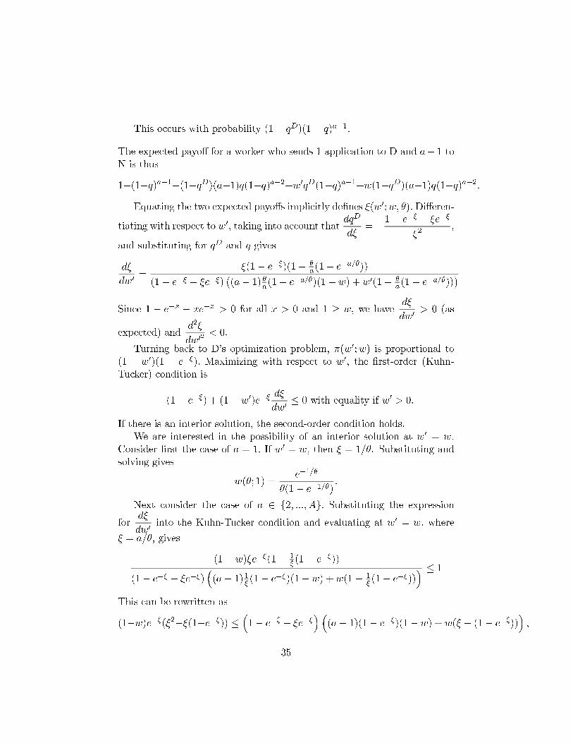
This occurs with probability (1− qD)(1− q)a−1.

The expected payoff for a worker who sends 1 application to D and a− 1 toN is thus

1−(1−q)a−1−(1−qD)(a−1)q(1−q)a−2+w′qD(1−q)a−1+w(1−qD)(a−1)q(1−q)a−2.

Equating the two expected payoffs implicitly defines ξ(w′;w, θ). Differen-

tiating with respect to w′, taking into account thatdqD

dξ= −

1− e−ξ − ξe−ξ

ξ2,

and substituting for qD and q gives

dξ

dw′=

ξ(1− e−ξ)(1− θa(1− e−a/θ))

(1− e−ξ − ξe−ξ)((a− 1)θa(1− e−a/θ)(1−w) +w′(1− θ

a(1− e−a/θ)))

Since 1 − e−x − xe−x > 0 for all x > 0 and 1 ≥ w, we havedξ

dw′> 0 (as

expected) andd2ξ

dw′2< 0.

Turning back to D’s optimization problem, π(w′;w) is proportional to(1 − w′)(1 − e−ξ). Maximizing with respect to w′, the first-order (Kuhn-Tucker) condition is

−(1− e−ξ) + (1−w′)e−ξdξ

dw′≤ 0 with equality if w′ > 0.

If there is an interior solution, the second-order condition holds.We are interested in the possibility of an interior solution at w′ = w.

Consider first the case of a = 1. If w′ = w, then ξ = 1/θ. Substituting andsolving gives

w(θ; 1) =e−1/θ

θ(1− e−1/θ).

Next consider the case of a ∈ {2, ...,A}. Substituting the expression

fordξ

dw′into the Kuhn-Tucker condition and evaluating at w′ = w, where

ξ = a/θ, gives

(1−w)ξe−ξ(1− 1

ξ (1− e−ξ))

(1− e−ξ − ξe−ξ)((a− 1)1ξ (1− e−ξ)(1−w) +w(1− 1

ξ (1− e−ξ))) ≤ 1

This can be rewritten as

(1−w)e−ξ(ξ2−ξ(1−e−ξ)) ≤(1− e−ξ − ξe−ξ

)((a− 1)(1− e−ξ)(1−w) +w(ξ − (1− e−ξ))

),

35

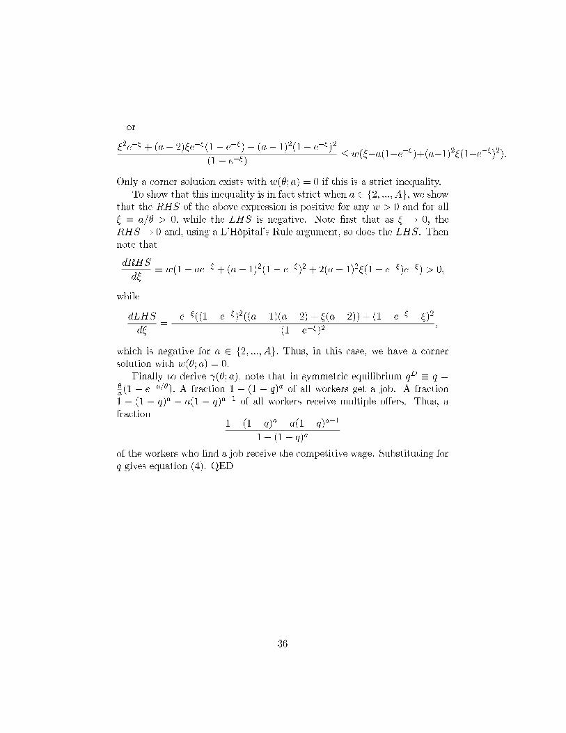
or

ξ2e−ξ + (a− 2)ξe−ξ(1− e−ξ)− (a− 1)2(1− e−ξ)2

(1− e−ξ)≤ w(ξ−a(1−e−ξ)+(a−1)2ξ(1−e−ξ)2).

Only a corner solution exists with w(θ;a) = 0 if this is a strict inequality.To show that this inequality is in fact strict when a ∈ {2, ..., A}, we show

that the RHS of the above expression is positive for any w > 0 and for allξ = a/θ > 0, while the LHS is negative. Note first that as ξ → 0, theRHS → 0 and, using a L’Hôpital’s Rule argument, so does the LHS. Thennote that

dRHS

dξ= w(1− ae−ξ + (a− 1)2(1− e−ξ)2 + 2(a− 1)2ξ(1− e−ξ)e−ξ) > 0,

while

dLHS

dξ=−e−ξ((1− e−ξ)2((a− 1)(a− 2) + ξ(a− 2)) + (1− e−ξ − ξ)2

(1− e−ξ)2,

which is negative for a ∈ {2, ...,A}. Thus, in this case, we have a cornersolution with w(θ; a) = 0.

Finally to derive γ(θ;a), note that in symmetric equilibrium qD ≡ q =θa(1 − e−a/θ). A fraction 1 − (1 − q)a of all workers get a job. A fraction1 − (1 − q)a − a(1 − q)a−1 of all workers receive multiple offers. Thus, afraction

1− (1− q)a − a(1− q)a−1

1− (1− q)a

of the workers who find a job receive the competitive wage. Substituting forq gives equation (4). QED

36