Chemistry. - "Equilibria in systems. in which phases. separated by a semi~permeable membrane." XIV. - By F. A. H. SCHREINEMAKERS.

(Communicated at the meeting of January 30. 1926).

Deductian af same properties af isatanic curves in ternary systems. In

which dimixtian inta twa liquids accurs.

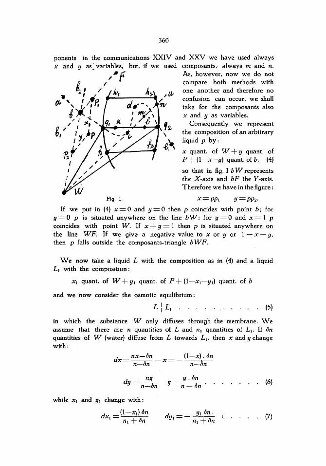
In order to deduce and to e1ucidate further the properties. discussed in the previous communicatian we cantemplate fig. I in which fl ql hl and f2 q2 h2 represent a part af the binadalcurve. The isotonic W~curve going through the two conjugated points is represented by the dotted curve ab ql cd q2 e. We are ab Ie to represent the composition. the thermodynamical potentiaI. etc. of an arbitrary phase Q. which contains the components W X and Y. not only with the aid of the quantities of those three components. but also with the aid of three arbitrary other phases (provided that they are not situated on a straight line); previously we have called those phases "composants" in distinction with the com~ ponents. of which this phase Q consists I).

As many properties can be deduced more easily with the aid of com~ posants than of components. we now shall use those composants.

We choose as composants I. the diffusing substance W. 2. an arbitrary liquid b. 3. an arbitrary phase F. As we have seen formerly (1. c.) we can represent the composition of an arbitrary liquid p by:

m quantities of W + n quantities of F + (I-m-n) quantities of b (I)

so that we call b as fundamental composant. Consequently we have in fig. I a system of coordinates with the point b as origin and the lines b Wand b F as axes. If we draw in the figure the lines p PI and p P2 parallel to b Wand b F th en is (1. c.)

m= PPI bW

n - PP2 -bF ' (2)

If we take for m as unity of leng th bW and for n as unity of length bF th en we can put:

m=PPI n =PP2 . (3)

In order to represent the composition of a liquid with the aid of com~

I) For a contemplation more in detail of components and composants comp.: In-. mono­and plurivariant equilibria. Comm. XXIV and XXV.

360

ponents in the communications XXIV and XXV we have used always x and Y as~variables. but. if we used composants. always mand n.

~ • f As. however. now we do not IJ ~ compare both methods with ~l ' / one another and therefore no

.. '.. confusion can occur. we shall Ol " " /, P. take for the composants also

I ';i:.. ~ x and Y as variables. /" / ". ..... f:1, Consequently we represent

g, ~ 1 \I jp \ the composition of an arbitrary

I ;/ .e~ liquid P by:

1) ,lt p, x quant. of W + Y quant. of {l r ~ F + (l-x-y) quant. of b. (4)

so that in fig. I bW represents the X-axis and bF the Y-axis. Therefore we have in the figure :

Fig. I. X=PPI y=PP2'

If we put in (4) x = 0 and y = 0 th en P coincides with point b; for y = 0 P is situated anywhere on the line bW; for y = 0 and x = I P coincides with point W. If x + y = I then P is situated anywhere on the line WF. If we give a negative value to x or y or I - x - y. then P falls outside the composants-triangle b WF.

We now take a liquid L with the composition as in (4) and a liquid LI with the composition:

XI quant. of W + YI quant. of F + (l-XI-YI) quant. of b

and we now consider the osmotic equilibrium:

L \ LI . ' (5)

in which the substance W only diffuses through the membrane. We assume that there are n quantities of Land nl quantities of LI' If lJn quantities of W (water) diffuse from L towards LI' th en x and Y change with:

dx= nx-lJ~ _ x = _ (I-x) . lJn n-lJn n-3n

d - ny _ y.lJn

y - n-lJn - y - n - lJn

while XI and YI change with:

dXI =(I-xI) !5n nl + lJn

d - _ YIlJn . YI - nl + lJn

(6)

(7)

361

The total thermodynamical potentialof the osmotic system (5) now changes with:

(n-bn) (C + ààC dx + aal dY) + (n + (~n) (Cl + aacl dXI + aa cl

d y l )-x Y XI YI • (8)

-nC - nl Cl in which C and Cl represent the thermodynamical potentials of the liquids Land LI' With the aid of (6) and (7). (8) passes into:

Cl +(1-xI) - -YI - -C-(I-x)-'--+y - (~n [ àCI aCI at aCJ aXI àYI ax ay (9)

As the thermodynamical potentialof a system in equilibrium is not allowed to change. (9) must be zero for infinitely small positive and negative values of an. Consequently the osmotic system (5) is in equili~ brium if:

t + (I-x) ac _ y at = [c + (I-x) ac _ y àC ·, ' ax ày àx àY _ I

. . (10)

The a. W. A. (osmotic water attraction) of an arbitrary liquid is defined therefore by:

at àt rp = t + (I-x) --" - y --' . ax ày

(11)

Previously (Comm. 11) we have found. using components for the a.W.A.

àt ac cp =C-x -- -y - ; ax ay the ongm of the system of coordinates was situated then in point W and now in the point b.

We now replace the liquid LI of equilibrium (5) by the liquid b of fig. 1; we then have the osmotic equilibrium:

L : Lb (fig . 1) · (12)

As XI and YI for liquid b are zero. it follows from (10) that the liquid L is defined by:

C + (1-x) - - y - = C + - . àC ac [ aCJ àx ày àx b

which represents the equation of the isotonic curve point b. From (13) follows :

[(I-x) r-ys] dx + [(I - x) s- yt] dy = 0

in which: a2t s = -_· axay

· (13)

going through

· (14)

362

If we take the liquid L of equilibrium (12) in the vicinity of the point b (fig. 1) th en x and y approach zero. r s and trest fini te. if b represents a ternary liquid. (14) now passes into:

rdx+sdy=O r

s (15)

by which the direction of the iso tonic curve in point b is defined. Of course this relation is valid for every arbitrary point of an isotonic curve. f. i. for the points a. q. c. d. q2' e etc. but not for its terminating~ points on the sides of the components~triangle.

As is known from the theory of the ternary liquids. outside the reg ion of dimixtion is:

rt-s2 > 0 (16)

This is also the case on the binodalcurve itself. Within the reg ion of dimixtion however a curve (not drawn in the figure) proceeds. on which :

rt-s2 =O . (17)

This is the spinodalcurve. which is situated within the binodalcurve. but touches this in the critical points. Within this spinodalcurve is:

rt- S2 < 0

and also may be r < 0 and t <' o. Is one of the magnitudes r or t negative. th en r t_s2 is negative also; of course the reverse is not the case.

If k and I in fig. 1 represent the points of intersection of the spinodal~ curve with the line ql q2' th en r t_s2 is zero in those points. therefore; between ql and k and q2 and I it is positive and between k and I negative.

The direction of the isotonic curve is defined by (15) in the point b; as b is situated outside the reg ion of dimixtion. r is > o. but the sign of s is indefinite. If s is negative. then it follows from (15) that the isotonic curve is situated in the vicinity of the point b within the angle W b F (and its opposite angle bI b b2); if s is positive. then the curve is situated within the angles bI b Wand b2 b F. If s = 0 then the curve touches in point b the Y~axis viz. the Hne b F. As r is never zero in the point b. the curve can. therefore. never touch the X~axis viz. the line b W in b.

Above we have seen already that (15) is true for every arbitrary point of an isotonic curve; as in every point outside the reg ion of dimixtion ris> O. none of the Hnes Wa. Wq\. Wq2 and We can touch this curve. therefore. Hence follows the property. already discussed before:

the part of an isotonic W~curve. situated outside a region of dimixtion has such a form that every straight Hne. going through point W. inter~ sects this curve in one point only and never touches it.

We now consider the part q\ cd q2 of the iso tonic curve. situated

363

within the region of dimixtion and we assume that r is zero in the points c and d and is negative. therefore. between c and d. It now follows from (15) that the isotonic curve touches the lines Wc and W din c and d. If we imagine within the angle c W d a straight line going through point W. th en this intersects the isotonic curve in th ree points. Consequently we find:

the part of an isotonic W~curve. situated within a region of dimixtion can have such a form that we are able to draw from point W straight lines which touch this branch or intersect it in three points.

If r is positive in all points of the part of the isotonic curve. situated between ql and q2. th en for this part the same is true as for the part. which is situated outside the region of dimixtion. This is the case f. i. with the curves 4 and 6 of fig 1. (Comm. XIII).

In order to examine the binodal~curve in the vicinity of the points ql and q2 we take as composants ql q2 and W. we represent the com~ position of two arbitrary liquids LI and L2 by:

XI quant. of W + YI quant. of q2 + (l-xI-YI) quant. of ql X2 quant. of W + Y2 quant. of q2 + (1-X2-Y2) quant. of ql.

Consequently we take a system of coordinates with point ql as origin ql W as X-axis and ql q2 as Y~axis. If LI and L 2 are two conjugated liquids. th en the equilibrium LI + L2 is defined by the three equations:

( C_XOC

_ Y OC)=(C_XOC

_ Y OC) ! ox oY I ox oY 2

(~:} (~:)2 (~~} (~~)2 (18)

We find those equations by expressing that the total thermodynamical potentialof the equilibrium LI + L 2 does not change. if small quantities of each of the three components ql q2 and W pass from the one liquid into the other. It follows from (18):

(xr+ YS)I dXI + (xs+ Y t)1 dYI = (xr+ Y sh dX2 +(xs+ Y th dY2 (19)

rl dXI + SI dYI = r2 dX2 + S2 dY2

SI dXI + tI dYI = S2 dX2 + t2 dY2

We now let coincide the liquids LI and L2 with the therefore we have to put:

(20)

(21)

points ql and q2;

XI=O YI=O Y2 = 1 . (22)

IE we substitute those values in equations (19) and if we neglect the terms of higher order than the first. we find:

o = S2 dX2 + t2 dY2 (23) The binodal-curve in the vicinity of the points ql and q2 is defined.

therefore. by (20). (21) and (23). Instead of (21) we now may write also:

(24)

364

If we substitute in (20) the va lues of dYI and dY2 which follow from (24) and (23) th en we find :

2 2 rltl-sld _r2 t2- s2 dx --- XI- 2

tI t2 (25)

Hence is apparent that dXI and dX2 have always the same sign. This means : if a liquid is situated on ql hl (ql fl) then the conjugated liquid is situated on q2 h2 (q2 {;).

Equation (24) defines the direction of the binodal curve in the point ql ; we have viz.:

(26)

The direction of the isotonic curve is defined in every point by (15). in the point ql therefore. we have to give to rand S in (15) the va lues rl and SI ' We th en have :

(27)

the first of which defines the direction of the isotonic curve. the second defines the direction of the binodal curve in the point ql' As rl and tI are positive. rl : SI and SI; tI have always the same sign. therefore. If SI = 0 th en follows:

dy =00

dx

It now follows from (29) and (28) :

(28)

the binodal curve and an isotonic curve are situated in the vicinity of their point of intersection either both within the conjugation-angle or both within the supplement-angle. If the binodal curve touches the one leg of the angle. th en the isotonic curve touches the other leg.

The O . W. A . of an arbitrary liquid L is defined by (11). For a Iiquid in the vicinity of L is true. therefore:

d ep = [(1 - x) r - y s] dx + [(1 - x) S - Y t] dy (29)

If we take the liquid L in the point ql (fig. 1) and if we take again the same components as above. consequently ql as origin of the system of coordinates. th en x and y become zero. (29) then passes into:

d ep = rl dx + SI dy . (30)

If we proceed from ql along the binodal curve towards a point in the immediate vicinity. th en the relation (24) is true for dx and dy. Hence follows for (30):

(31)

365

in which the coefficient of dx is positive. We now proceed from ql in the direction towards hl or. as we have expressed it in the previous communication : we proceed starting from the point ql along the binodal curve away from point W. As then dx is negative. dep. therefore. is also negative and consequently the O . W. A. increases. Therefore we find:

the O . W. A. of the liquids of a binodal curve increases in that direction in which we move away from the point W.

We have already applied this property in order to define the direction in which the O. W . A . of the liquids increases along the binodal curve of the figs. 1-3 (previous Communication).

In the previous Communication we have discussed already. that the isotonic curve. which goes through mI (figs 2 and 3 Comm. XIII). touches the binodal curve in this point mI. A second branch of the isotonic curve. which is situated. however. totally within the region of dimixtion. also touches the binodal curve in the point m2.

In order to examine the isotonic curve and the binodal curve in the vicinity of those points. we take as composants: W mI and an arbitrary phase F. Consequently we take a system of coordinates with mI as origin. mI W as X-axis and mI F as Y-axis.

For the isotonic curve. going through point mI ' equation (15) is true. in which we have to give to C and S the values. which they have in mI.

If we take those Cl and SI' then curve 2 (fig . 2 XIII) and curve 5 (fig. 3 XIII) in the vicinity of mI are defined by:

dy_ Cl

dx SI (32)

For an equilibrium LI + L 2 the equations (18) are true and the equations (19)-(21) which follow from this. We now imagine the liquids LI and L2 in the points mI and m2. so that:

XI =0 YI =0 Y2=0. (33)

Limiting ourselves to terms of the first order. then (19)-(21) pass into:

o = X2 (C2 dX2 + S2 dY2)

Cl dXI + SI dYI = C2 dX2 + S2 dY2

SI dXI + tI dYI = S2 dX2 + t2 dY2.

Hence follows:

(34)

by which the direction of the binodal curve in mI is defined. It is apparent Erom (32) and (34) that the isotonic curve and the binodal curve touch one another in mI.

If we take as composant m2 instead of mI. then we have to exchange

366

the indices 1 and 2 in the deduction above. hence follows that the isotonic curve and the binodal curve touch one another also in the point m2

(6gs. 2 and 3 XIII).

The change of the O. W.A. of a liquid L is de6ned by (29); therefore is true for the liquid mI (6g. 2 and 3 XIII):

dg; = [(1 - XI) rl - YI sd dXI + [(1 - XI) SI - YI td dYI . (35)

As however XI = 0 and YI = O. (35) passes into:

dg; ='1 dXI + SI dYI' (36)

We now choose the new liquid on the binodal curve so that dXI and dYI satisfy (34); th en follows:

(37)

Hence follows the property. already formerly discussed: the O. W. A. of the liquids of a binodal curve is maximum or minimum

in the points. which are situated on the conjugation~line going through W (6gs. 2 and 3 XIII).

We have assumed in the deductions above that the points mI and m2

represent ternary liquids. so that mI m2 is a ternary conjugation~line. If. however. mI and m2 are binary liquids. then the deductions are

valuable no more. If we imagine the line W mI m2 (6gs. 2 and 3 XIII) coinciding with one of the sides of the components~triangle. then tI and t2

are in6nitely large. but YI tI and Y2 t2 rest 6nite for YI = 0 and Y2 = O. It now follows from (19) - (21):

YI tI dYI = X2 (r2 dX2 + S2 dY2)! rl dXI + SI dYI = r2 dX2 + S2 dY2

tI dYI = t2 dY2 . (38)

while (14) which de6nes the direction of the iso tonic curve. passes into:

rl dx + (SI - YI td dy = 0 . (39)

From (38) follows for the binodal curve

rldXI+(SI-Y~:I)dYI=O (40)

It is apparent from (39) and (40) that the isotonic curve and the binodal curve do not touch one another now, a property to which we have pointed in the previous communication.

Above we have seen that the O. W. A. of the liquids of the binodal curve in the points mI and m2 (6gs. 2 en 3 XIII) is a maximum or minimum; we now shall consider this case more in detail.

We have represented the compositions of the liquids with the aid of the composants Wml and F. in which F is an arbitrary phase. We now choose F in such a way that SI becomes = O. (Later on it will

367

appear that F is situated then anywhere on the tangent going through point mi)' If we involve in (19) ~ (21) also terms of higher order and if we put:

th en we get:

~ rl dx~ + ~ ti dy~ = X2 (r2 dX2 + S2 dY2) + A 2

rl dXI + ~ ~~II dyî = r2 dX2 + S2 dY2 + B2 .

ti dYI + Cl = S2 dX2 + t2 dY2 + C2 • •

(il)

(i2)

(i3)

(44)

In the first part of (i3) the terms with dXI dYI and dxî. which are infinitely small with respect to dXI' are omitted. A. Band C contain the terms of the second order. We can satisfy those equations by taking dYI dX2 and dY2 of the same order and dXI of the order dyî. while r2 dX2 + S2 dY2 is also of the order dyî. Consequently we may write for {i2)-(ii) :

~ ti dyî = X2 (r2 dX2 + S2 dY2) + A 2 .

1 OSI 2 B rl dXI + 2 àYI dYI = r2 dX2 + S2 dY2 + 2

ti dYI = S2 dX2 + t2 dY2 . Herein is:

(iS)

(i6)

(i7)

1 ( à r) ( ar) 1 ( àS) A 2 = 2 r + x àx 2 dx~ + S + x ày 2 dX2 dY2 + 2 t + x ày dy~ (i8)

B - 1 àr2 d 2 àr2 d d 1 OS2 2 2 - -2 ~ x 2 + ~ X2 Y2 + -2 ~ dY2

UX2 UY2 UY2

It follows from (iS) and (i6):

· (i9)

rl dXI +l (à SI -~) dyî = _l (1 r dX2 + S dxdy + t dy2). (50) 2 ~I ~ ~ 2 2

It follows from (i6) and (i7):

· (51) in which:

D= r2 t2 - s~.

The terms of higher order are neglected in (51); if we substitute the values of dX2 and dY2 from (51) in the second part of (50), then we find:

d +l (àSI_~+ tî r2 )d 2_ 0 rl XI 2 À D yl - •

UYI X2 X2 · (52)

by which the binodal curve is defined in the vicinity of the point In a similar way we find from (1 i) for the isotonic curve:

1 (àS I ) 2_ rl dX+ 2 àYI - ti dy -0 .. . . (53)

368

and for the change of the O. W. A. from (35):

dep=c, dx, +~ (~;:-t,)dY~ (54)

We now choose dx, and dy, in such a way that the new liquid is situated on the binodal curve; consequently dx, and dYI must satisfy (52); then we may replace (54) by:

(55)

Instead of by (37) dep is defined. therefore. by a magnitude of the second order. With the aid of (51) we are able to give still another form to (55). viz.:

1 ( dY2) ti d 2 dep= - l-X2- - -. YI. 2 dYI X2

(56)

It follows from (52) and (53) that the binodal curve and the isotonic curve are parabolic in the vicinity of mI and touch both the Y~axis in m I ' In order to define the position of those curves with respect to one another. we imagine in the figures to be drawn a line m; W;. parallel to and in the vicinity of m, W. For the point of intersection of m; W; with those curves then is valid dy = dYI' It follows then from (52) and (53) :

If we put:

~Sl_tl =_ QI UYI

th en we may write (57) with the aid of (55) :

(57)

(58)

dep dx dXI -dx=2d~'-Q (59)

YI 1

If we consider the value of QI from (58). th en follows from (53) that dx and QI have the same sign. so that dx: QI is always positive; the sign of (59) is the same. therefore. as that of dep.

In order to apply the above equations. we shall distinguish different cases:

A. Binodal curve and isotonic curve in mi; fig. 2 XIII. The origin of the system of coordinates is situated. therefore. in point

mi of the figure. If we imagine the conjugation~line al a2 in the vicinity of mI m2. th en we find:

al mi> a2 m2 Wml Wm2

. (60)

As al mi = dYI' a2m2 = dY2' Wml = 1 and Wm2 = I-x2 in

369

which x is negative. therefore. we may write for (60). if we take positive dgl and dg2• also

or: dg2 l- x2-->0 dgl

If we take dgl and dg2 both negative. then we find also (62). As X2 is negative. it follows from (56):

(61)

(62)

dg; < 0 . (63)

Consequently g; is a maximum in mI ; the O. W . A . is a minimum in mI. therefore. This is in accordance with the direction of the arrows on the binodal curve (fig. 2 XIII). It now follows from (59) in connec~ tion with (63):

(64)

This means : if we proceed along the line m; W; (see above) in the direction towards the point W . then we meet firstly the binodal curve and afterwards the isotonic curve; we see th at this is in accordance with the figure.

B. Binodal curve and isotonic curve in mI; fig. 3 XIII. The origin of the system of coordinates is situated. therefore. in point

mI of the figure; X2 is positive now. In the same way as in A we find again (62) ; as. however, X2 is positive, it now follows :

(65)

In accordance with the direction of the arrows in the figure. it follows, therefore. that the O . W. A . in mI is a maximum. In connection with (65) it follows from (59) :

(66)

This is in accordance with the position of the binodal curve and the isotonic curve in the vicinity of point mI '

In order to conslder the curves in the vicinity of the point m2' we may use also the equations (52)-(59); then. however, we have to replace the index 1 by 2 and X2 by XI' We call those new equations (52a)-(59"); with the aid of (60) we find instead of (62):

(67)

We now distinguish two cases. C. Binodal curve and isotonic curve in m2; fig. 2 XIII. The origin of the system of coordinates is situated now in the point

m2 of the figure ; XI is positive but smaller than 1. With the aid of (67) 25

Proceedings Royal Acad. Amsterdam. Vol. XXIX.

370

we find from (56a) that d q; < O. which is in accordance with (63). as is necessary.

Instead of (64) we find from (59-):

. (68)

This is in accordance with the position of the two curves in the vicinity of point m2 ; the branch of the iso tonic curve which touches the ·15inodal curve in m2 is situated viz. within the region of dimixtion.

D. Binodal curve and isotonic curve in m2; fig . 3 XIII. The origin of the system of coordinates is situated now in the point

m2 of the figure; XI is negative. With the aid of (67) we now find from (568

) that d q; > O. This is in accordance with (65). Instead of (66) now is:

(69)

This is also in accordance with the figure; the branch of the isotonic curve. which touches the bino:ial curve in m2. is situated viz. within he region of dimixtion.

(Ta be continued).