Embed Size (px)
Citation preview
Theoretical Computer Science 285 (2002) 487–517www.elsevier.com/locate/tcs
Equational rules for rewriting logicPatrick Viry∗
ASTEM RI, 17 Chudoji Minami-machi, Shimogyo-ku, Kyoto 600-8813, Japan
Abstract
In addition to equations and rules, we introduce equational rules that are oriented while havingan equational interpretation. Correspondence between operational behavior and intended seman-tics is guaranteed by a property of coherence, which can be checked by examination of criticalpairs and linearity conditions. We present applications of this theory to three examples wherethe rewrite relation is interpreted, respectively, as equality, transition and deduction. c© 2002Elsevier Science B.V. All rights reserved.
Keywords: Rewriting; Equational programming; Coherence; Building-in equality
1. Introduction
Rewriting logic [31] can be thought of as one of the most general logical frameworks,in the sense that all logical systems found in practice can be mapped in a simple wayinto a rewriting logic theory [29]. A major reason of this success is that rewriting logicdoes not impose any implicit structure on the objects to be represented: all structuremust be explicitly de9ned using equations.A rewrite theory mainly consists of a set of oriented rules R and a set of non-oriented
equations E. Operationally, the sequent s→ t is valid in the rewrite theory (E; R) i;there is a derivation from s to t by rewriting with the rules of R modulo E. Equationsin E can be thought of as specifying the structure over which rules of R operate. Thesemantics of rules in R is not 9xed ; depending on the application, a rewrite step canbe interpreted for instance as a transition between states (e.g. automata, processes),as a logical deduction (e.g. sequent calculus) or as equality (e.g. �-reduction in the�-calculus).
∗Corresponding author. Present address: ILOG S.A., B.P. 85, grue de Verdun, 94253 Gentilly Cedex,France.
E-mail address: [email protected] (P. Viry).
0304-3975/02/$ - see front matter c© 2002 Elsevier Science B.V. All rights reserved.PII: S0304 -3975(01)00366 -8
488 P. Viry / Theoretical Computer Science 285 (2002) 487–517
Let us take a closer look at this dichotomy between rules and equations:• from a semantic point of view, the equations in E are always given an equationalsemantics, but it is not necessarily so for the rules in R.• from an operational point of view, the rules in R can be used only according to theirorientation, while the equations in E are not oriented.
These two aspects are often conBicting, and choosing between specifying somethingas a rule or an equation can be a dilemma. In particular, when E is not tractabledirectly, classical rewriting techniques can replace all or part of E by oriented rewriterules, mapping equivalence classes to their unique canonical representative. But doingso implies adding these rules to R, where they lose their equational semantics.A solution to this dilemma is to introduce a second set of rules ER (for “Equational
Rules”, denoted with =→), which are oriented but keep an equational semantics. Con-sider the following example, which may be thought of as specifying a double function(f) and a non-deterministic choice operator (?) over the natural numbers:
E R
(1) x + y = y + x(2) 0 + x = x(3) s(x) + y = s(x + y)
(4) f(x) → x + x(5) ? → 0(6) ? → 1
R is not interpreted equationally, hence the rules for non-deterministic choice do notimply 0=1. In order to handle E more eHciently, one may wish to orient Eqs. (2)and (3) into equational rules, changing their operational meaning (they ought to beused only according to their orientation), while preserving their equational semantics(0 + x is equal to x).For semantic considerations, one may wish also to transform rule (4) into an equa-
tional rule, keeping its operational meaning while giving it an equational semantics.The resulting oriented rewrite theory (E; ER; R) is
E ER R
(1) x + y = y + x(2) 0 + x =→ x(3) s(x) + y =→ s(x + y)(4) f(x) =→ x + x
(5) ? → 0(6) ? → 1
2. Structure of the paper
After introducing some basic concepts (Sections 3 and 4), we formally de9ne thenotion of an oriented rewrite theory in Section 5.The central notion appearing in this framework is the property of coherence
(Section 5.1), which ensures a correspondence between operational behavior and in-tended semantics. We show how to check coherence (Sections 5.2 and 5.3), and possi-bly obtain it through coherence completion (Section 5.5). Section 6 extends the previousresults to the case of conditional rules.
P. Viry / Theoretical Computer Science 285 (2002) 487–517 489
In Section 7, we show how the techniques of [23] for implementing rewriting mod-ulo E using matching modulo E can be extended to the case of an oriented rewritetheory.In Section 8, we develop an example showing how the coherence techniques may
help replacing a non-terminating rewrite relation by a terminating one.The rest of the paper is devoted to examples. We present three examples, corre-
sponding to the most usual interpretations of the rewriting relation:(1) Equational semantics (Section 9): Example of calculi with bound variables,
whose main representative is the �-calculus. Substitution is usually considered an im-plicit meta-operation, but a full 9rst-order speci9cation requires to make it explicitusing a substitution calculus. The substitution rules are oriented rules, with an equa-tional semantics (i.e. part of the internal structure).(2) Transition semantics (Section 10): A rewrite step is interpreted as a transition
between states, the structure of a state being speci9ed by E and ER. A typical exampleis a process algebra, in the spirit of CCS [33]. Building on the treatment of boundvariables developed above, we present the example of the �-calculus [34].This example can be extended by specifying the actual data exchanged by processes
as abstract data types, in a manner similar to LOTOS [5], thus having the transitionsemantics and data types speci9ed in a single framework.(3) Deduction semantics (Section 11): A rewrite step is interpreted as a logical de-
duction between propositions. By varying the structure of propositions, we can specifyfor instance classical logic or linear logic (including or not the weakening axioms inE). Here moving a rule from R to ER can be seen as the building-in of equality.Most of the material presented here originates from [38,39,40,41,42]. Some changes
and additions have been introduced, in particular a new de9nition of local coherence(Section 5.2) that allows to get rid of a troublesome termination condition, and asection on conditional rules.The coherence checking and coherence completion techniques presented here have
been implemented in Maude [30] using the reBection features of this system, and arenow part of the standard distribution [14].
3. Basic concepts
3.1. Relations
Given a binary relation →, we denote ← its inverse, � its transitive and reBexiveclosure, ↔ its symmetric closure and �� its transitive symmetric and reBexive closure.The notation� is equivalent to the usual→∗, but makes diagrams much more readable.An element u is a →-normal form if there is no v such that u→ v. The normalizing
relation!� is de9ned as u
!� v if u� v and v is a →-normal form.
Given a rewrite system R= {li→ ri}, the rewrite relation R→ is the smallest relation
stable by context and instantiation containing liR→ ri for each li→ ri ∈R. For a set of
equations E= {ui = vi}, the replacement relation E↔ is de9ned similarly, and closed
490 P. Viry / Theoretical Computer Science 285 (2002) 487–517
by symmetry. [u]E denotes the equivalence class of u modulo E, i.e. [u]E is the set
{v|v E�� u}. Similarly, a set of rules R, when considered as equations, also de9nes
equivalence classes [u]R. For any relationsR→ and S→, de9ne
R=S→ =S� R→ S
�
In particular, when S→ is the replacement relation E↔ generated by a set E of equations,R=E−→ is the basis for de9ning rewriting over classes modulo E:
[u]E[R]E→ [v]E i; u
R=E→ v:
We use the abbreviations[R=S]E−→ for
[R]E=[S]E−→ =[S]E�
[R]E−→ [S]E� , and[R∪S]E−→ for
[R]E−→ ∪ [S]E−→.Finally, because it makes de9nitions and diagrams simpler, instead of
[R=S]E−→ we will
often use the relation[R(S)]E−→ de9ned as
[R(S)]E→ =[S]E�
[R]E→[S]E� steps are allowed only before the
[R]E−→ steps, but we have the following correspon-dence:
[R=S]E→ =[R(S)]E→ [S]E�
and for derivations[R=S]E� =
[R(S)]E�[S]E�
3.2. Diagrams
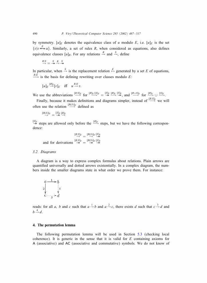
A diagram is a way to express complex formulas about relations. Plain arrows arequanti9ed universally and dotted arrows existentially. In a complex diagram, the num-bers inside the smaller diagrams state in what order we prove them. For instance:
reads: for all a; b and c such that a 1→ b and a 2→ c, there exists d such that c 3→d andb 4→d.
4. The permutation lemma
The following permutation lemma will be used in Section 5.3 (checking localcoherence). It is generic in the sense that it is valid for E containing axioms forA (associative) and AC (associative and commutative) symbols. We do not know of
P. Viry / Theoretical Computer Science 285 (2002) 487–517 491
any other case where this lemma is valid (it does not hold even for arbitrary shallowtheories [8]). Intuitively, the lemma relies on being able to identify positions in a term.For A and AC symbols, positions in Battened terms are considered.We do not consider this restriction to A and AC as a practical limitation, since
available rewrite interpreters such as OBJ [17], Maude [32,30] or ELAN [39,24] doprovide implementations only for rewriting modulo theories including the axioms ofassociativity, commutativity, identity and idempotency, and the last two axioms willnormally be considered as oriented equational rules.
De�nition 1 (Flattened terms [11]). A Battened term is a term [t]A considered moduloall associativity axioms in E (in the following we consider only Battened terms, in-cluding in rules, and abbreviate [t]A to t). It is possible to de9ne a notion of positionsPos(t) in Battened terms, depending on the properties of the topmost symbol f:• If f is a free symbol, then
Pos(f(t1; : : : ; tn) = {�} ∪n⋃
i=1{ip |p ∈ Pos(ti)}:
• If f is an A symbol, then
Pos(f(t1; : : : ; tn)) = {�} ∪ {[i; j] | 16 i ¡ j 6 n} ∪n⋃
i=1{ip |p ∈ Pos(ti)}:
• If f is an AC symbol, then
Pos(f(t1; : : : ; tn)) = {�} ∪P({1; : : : ; n}) ∪n⋃
i=1{ip |p ∈ Pos(ti)}:
The usual notions of substitution, stability by context and instantiation, rewriting, areeasily extended to Battened terms.
For instance, considering an AC symbol +, the rule a + c→d applies to the terma+ b+ c at position {1; 3}, giving b+ d as a reduct.
De�nition 2 (Extended critical pairs [27]). Extended critical pairs extend the usualnotion of critical pairs to Battened terms. Consider two Battened rules �1 : l1→ r1 and�2 : l2→ r2; there is a head superposition between l1 and l2 if Head(l1)=Head(l2)=fand there exists a substitution ! such that one of the three possibilities below holds:• f is a free symbol and l1!=E l2!• f is an A symbol and L1 =E L2, where L1 is either l1!; f(x; l1)!; f(x; l1; y)! or
f(l1; y)!; and L2 is either l2!; f(u; l2)!; f(u; l2; v)! or f(l2; v)!, with x; y; u; vbeing new variables.• f is an AC symbol and L1 =E L2, where L1 is either l1! or f(x; l1)!; L2 is either
l2! or f(u; l2)!, with x; u being new variables.Superpositions of l2 within l1 at position p �= � are de9ned similarly, considering forL1 only the case L1 = l1!.
492 P. Viry / Theoretical Computer Science 285 (2002) 487–517
The set CPE(�1; �2) of extended critical pairs is de9ned as usual considering allsuperpositions between l1 and l2. Note that in the presence of A symbols, the set ofcritical pairs may possibly be in9nite since A-uni9cation is not 9nitary [37].
For instance, considering an AC symbol +, the rules a+b→ c and a+d→ e inducethe critical pair (c + d; b + e). Taking != {x �→d; y �→ b}, we have (a+ b+ x)!=AC(a+ d+y)!=AC a+ b+ d.This de9nition of critical pairs is di;erent from the usual notion of critical pairs
modulo [23]: it takes into account the fact that rewriting is performed directly onBattened terms and in some sense internalizes the extension rules [35] that would beneeded if rewriting modulo were done on syntactic (non-Battened) terms.
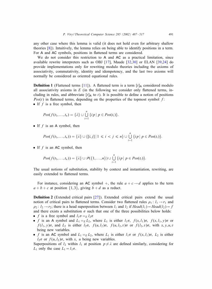
Lemma 3 (Permutation lemma). For an equational theory E containing only axiomsfor A and AC symbols, we have: for any two rules �1 : l1→ r1 and �2 : l2→ r2, and
any critical peak [s]E[�1]E←− [�2]E−→[t]E ,
• (Superposition case) either there is a critical pair (s; t)∈CPE(�1; �2),• (Non-superposition case) or the critical peak can be closed as follows
Moreover, if l2 is linear or if the l1→ r1 step is not below the l2→ r2 step, then thederivation (a) is empty. If r2 is linear or if the l1→ r1 step is not below the l2→ r2step, then the derivation (b) is a single step. Note that the notion of applying astep below another has to be understood in the context of :attened terms.
A proof for the case AC is given in [28]. With the de9nition of superposition forA symbols and the associated de9nition of extended critical pairs that we introducedhere, the same proof works by replacing =AC with =A when considering A symbols.Note that the notion of critical pairs modulo E proposed in [23] is not general enoughfor the permutation lemma to hold.
5. Oriented rewrite theory
Extending the notion of a rewrite theory of rewriting logic [31], we de9ne an orientedrewrite theory as a tuple ($; E; ER; R), where• $ is the signature upon which terms are built• E is a set of equations (u= v)∈T 2
$;X
P. Viry / Theoretical Computer Science 285 (2002) 487–517 493
• ER is a set of equational rules (u =→ v)∈T 2$;X
• R is a set of reduction rules 1 (u→ v)∈T 2$;X .
The case of conditional rules will be addressed later in Section 6. Compared to a“classical” rewrite theory, this de9nition makes room for two kinds of rules:• Rules of ER are always given an equational interpretation: the oriented rewritetheory de9nes equivalence classes modulo E ∪ER. We will always suppose that
the rules of ER form a rewrite system convergent modulo E (i.e.[ER]E−→ is conBuent
and terminating).• Rules of R are not necessarily interpreted equationally. They may be interpreted forinstance as transitions between states or deduction steps. However, nothing preventsgiving an equational interpretation to the reduction rules as well.In “classical” rewriting logic, the same semantics would be obtained by considering
ER rules as non-oriented equations. The idea behind the above de9nition is that eventhough rules of ER have an equational interpretation, they must be used only accordingto their orientation. Each of these considerations leads to a di;erent view:Operational view: “The rules of ER must be used according to their orientation”.
This leads to consider sequents for the rewrite theory (E; ER∪R):
[s]E[R(ER)]E→ [t]E
Semantic view: “The rules of ER have an equational semantics”. This leads to con-sider sequents for the rewrite theory (E ∪ER; R):
[s]E∪ER[R]E∪ER→ [t]E∪ER
These two relations are not equivalent. We have
[s]E[R(ER)]E→ [t]E ⇒ [s]E∪ER
[R]E∪ER→ [t]E∪ER
but the opposite is not true in general. As an example, consider
E = ∅; ER = {x + 0 =→ x}; R = {f(x + y)→ g(x) + g(y)}:
We have [f(x)]E∪ER[R]E∪ER−→ [g(x)+g(0)]E∪ER, since [f(x)]E∪ER= [f(x+0)]E∪ER, but
[f(x)]E is not reducible by[R(ER)]E−→ .
In the next section, we introduce di;erent notions of coherence. Strong coherenceis a suHcient condition for the above implication to be an equivalence, but may bediHcult to verify. Weaker notions of coherence correspond to weaker correspondences
between[R(ER)]E−→ and
[R]E∪ER−→ .Then in the following sections, we provide some techniques for checking or estab-
lishing these coherence properties.
1 In the original de9nition, rules may also be labelled.
494 P. Viry / Theoretical Computer Science 285 (2002) 487–517
5.1. Coherence
Depending on how close a correspondence we seek between the operational andsemantic views of oriented rewriting logic, we introduce three notions of coherence.• Strong coherence states that the exact number of steps of a derivation is preserved(one may wish also to impose that the same rule is used — or a rule generated bycompletion from the original one, see Section 5.5 — the results extend straightfor-wardly to this case).It is the property needed when one wishes to preserve the whole derivation space,
namely being able to identify single steps of the semantic view and of the operationalview, for instance when implementing automata or process algebras.• Weak coherence states that derivability is preserved, but not necessarily the inter-mediate steps.• Equational coherence states that the set of normal forms is preserved, except possiblyfor some cycles.This property makes sense mainly in an equational context (R equationally inter-
preted), where one is only interested in normal forms with respect to[R]E∪ER−→ . In such
a context,[R]E∪ER−→ is usually supposed to be conBuent.
Equational coherence is the most general property, it can be checked by looking atcritical pairs. Weak coherence may be more diHcult to establish in the presence ofnon-left-linear rules in R, and strong coherence in the presence of non-right-linear rulesas well. We will see suHcient conditions in the next sections.
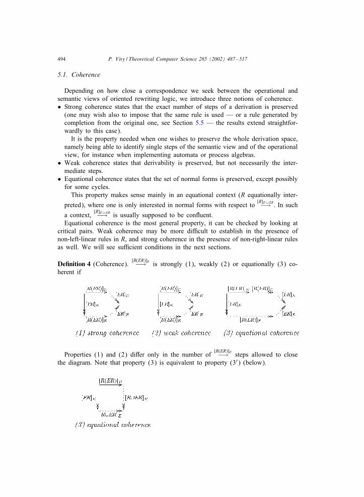
De�nition 4 (Coherence).[R(ER)]E−→ is strongly (1), weakly (2) or equationally (3) co-
herent if
Properties (1) and (2) di;er only in the number of[R(ER)]E−→ steps allowed to close
the diagram. Note that property (3) is equivalent to property (3′) (below).
P. Viry / Theoretical Computer Science 285 (2002) 487–517 495
The intuition behind the de9nition of these three notions of coherence is justi9ed bythe following theorem.
Theorem 5 (Coherence). Remember that we suppose[ER]E−→ convergent.
• If[R(ER)]E−→ is strongly coherent, then
[u]E∪ER[R]E∪ER→ [v]E∪ER ⇒ [u]E
[R(ER)]E→ [v′]E[ER]E��[v]E:
• If[R(ER)]E−→ is weakly coherent, then
[u]E∪ER[R]E∪ER� [v]E∪ER ⇒ [u]E
[R(ER)]E� [v′]E[ER]E��[v]E:
• If[R(ER)]E−→ is equationally coherent, then
if [u]E is a normal form for[R(ER)]E−→ , then either [u]E∪ER is a normal form for
[R]E∪ER−→ , or there is a non-empty cycle [u]E∪ER[R]E∪ER� [u]E∪ER.
In the case of equational coherence, the set of normal forms is not exactly preserved,
since a cycle in[R]E∪ER−→ may be matched by an empty derivation of
[R(ER)]E−→ . This is thereason why in the identity rewriting example (Section 8), a non-terminating relationmodulo AC1 can be simulated by a terminating relation, and the reason why we choosethis de9nition of equational coherence.If an exact correspondence between the sets of normal forms is required, the def-
inition of equational coherence has to be adapted in order to close the diagram with
at least one[R(ER)]E−→ step. This latter de9nition rules out the possibility of a non-empty
cycle.
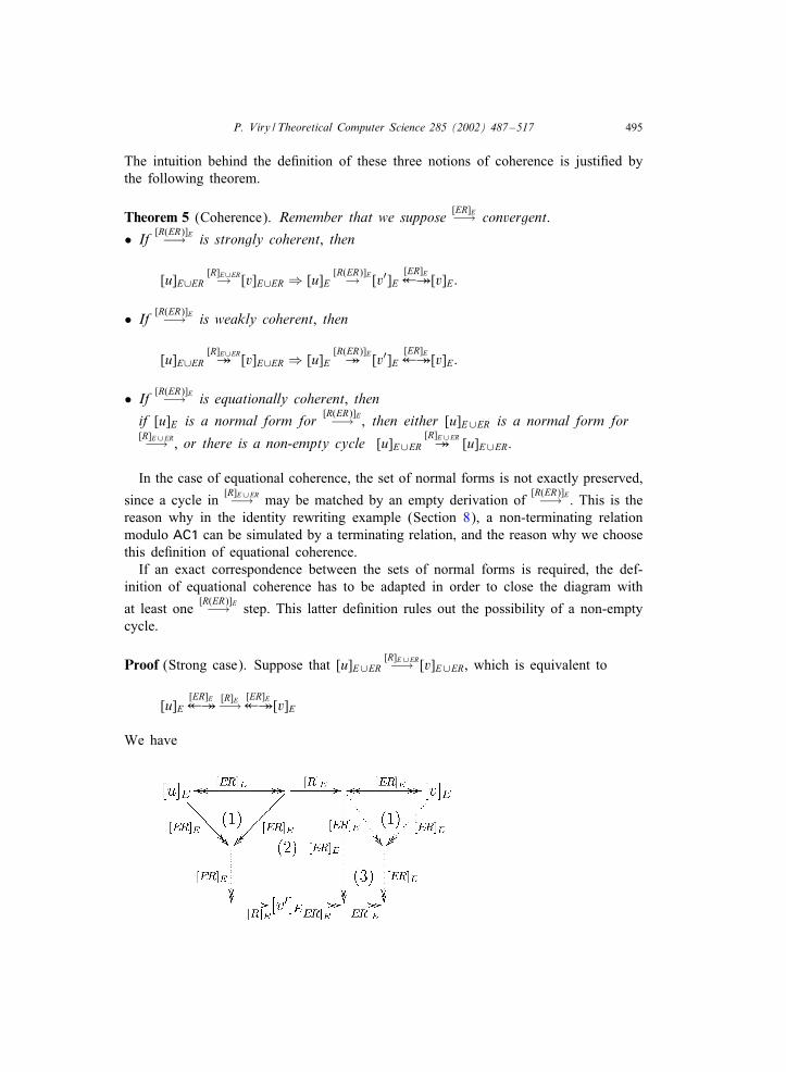
Proof (Strong case). Suppose that [u]E∪ER[R]E∪ER−→ [v]E∪ER, which is equivalent to
[u]E[ER]E��
[R]E−→ [ER]E��[v]E
We have
496 P. Viry / Theoretical Computer Science 285 (2002) 487–517
(1) conBuence of[ER]E−→
(2) strong coherence of[R(ER)]E−→
(3) conBuence of[ER]E−→.
Hence [u]E[R(ER)]E−→ [v′]E
[ER]E�� [v]E .
Weak case. Suppose that [u]E∪ER[R]E∪ER� [v]E∪ER, which is equivalent to
[u]E([ER]E��
[R]E→︸ ︷︷ ︸n
)∗[ER]E��[v]E:
We want to prove that [u]E[R(ER)]E�
[ER]E�� [v]E by induction over the number n of
[R]E−→steps in the derivation. Either n=0 and the theorem is trivially true, or we have
(1) conBuence of[ER]E−→
(2) weak coherence of[R(ER)]E−→
(3) induction hypothesiswith n− 1 R-steps
Hence [u]E[R(ER)]E�
[ER]E�� [v]E .
Equational case. Remember that [u]E[R]E−→ [v]E is de9ned as u
E�� R−→ E
�� v.
Suppose that [u]E is a normal form for[R(ER)]E−→ , namely there does not exist any v
such that [u]E[ER]E�
[R]E−→ [v]E , i.e. u(E�� ER−→ E
��)∗ R−→ E�� v.
Now consider a derivation [u]E[ER]E��
[R]E−→ [v]E , i.e. u(E�� ER↔ E
��)∗ R−→ E�� v, which
can be written in the more compact form uER=E�� R−→ E
�� v:
• If no such derivation exists, then [u]E∪ER is a normal form for[R]E∪ER−→ , by de9nition.
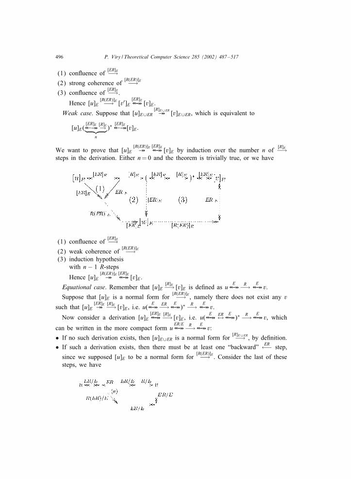
• If such a derivation exists, then there must be at least one “backward” ER←− step,
since we supposed [u]E to be a normal form for[R(ER)]E−→ . Consider the last of these
steps, we have
P. Viry / Theoretical Computer Science 285 (2002) 487–517 497
by equational coherence. Since we supposed that [u]E is a normal form for[R(ER)]E−→ ,
the derivation (a) is empty, hence there is a derivation uE∪ER�� v, which means that
[u]E∪ER= [v]E∪ER and there is a cycle [u]E∪ER[R]E∪ER−→ [v]E∪ER.
This ends the proof of Theorem 5.
5.2. Local coherence
In order to be able to check coherence syntactically (by looking only at the rewrite sys-temsR andER),we9rst de9ne the local versions of strong,weak and equational coherence:
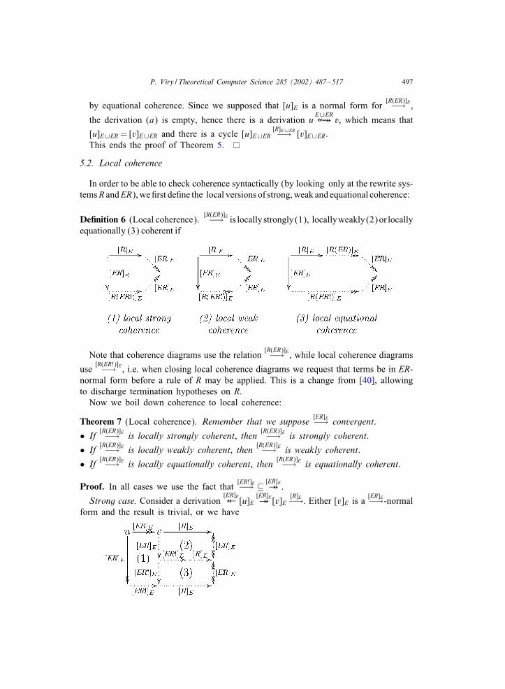
De�nition 6 (Local coherence).[R(ER)]E−→ is locallystrongly(1), locallyweakly(2)or locally
equationally (3) coherent if
Note that coherence diagrams use the relation[R(ER)]E−→ , while local coherence diagrams
use[R(ER!)]E−→ , i.e. when closing local coherence diagrams we request that terms be in ER-
normal form before a rule of R may be applied. This is a change from [40], allowingto discharge termination hypotheses on R.Now we boil down coherence to local coherence:
Theorem 7 (Local coherence). Remember that we suppose[ER]E−→ convergent.
• If[R(ER)]E−→ is locally strongly coherent, then
[R(ER)]E−→ is strongly coherent.
• If[R(ER)]E−→ is locally weakly coherent, then
[R(ER)]E−→ is weakly coherent.
• If[R(ER)]E−→ is locally equationally coherent, then
[R(ER)]E−→ is equationally coherent.
Proof. In all cases we use the fact that[ER!]E−→ ⊆ [ER]E� .
Strong case. Consider a derivation[ER]E� [u]E
[ER]E� [v]E[R]E−→. Either [v]E is a [ER]E−→-normal
form and the result is trivial, or we have
498 P. Viry / Theoretical Computer Science 285 (2002) 487–517
(1) convergence of[ER]E−→
(2) local strong coherence
(3) uniqueness of[ER]E−→-normal forms
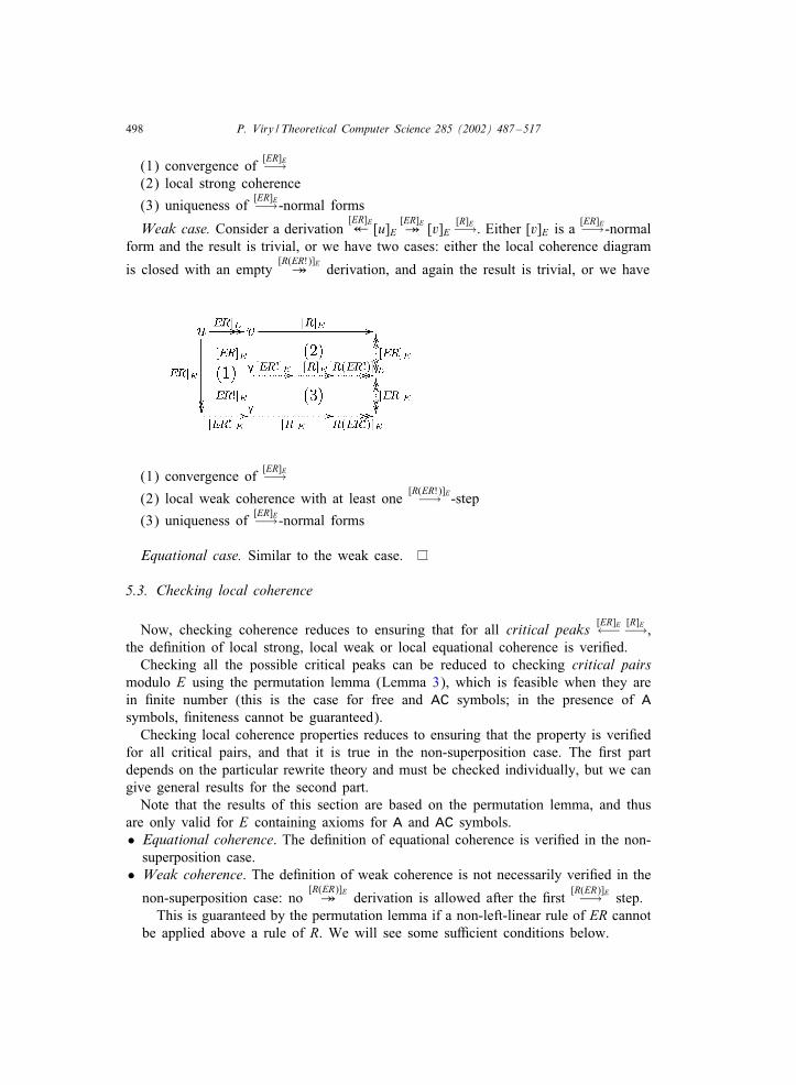
Weak case. Consider a derivation[ER]E� [u]E
[ER]E� [v]E[R]E−→. Either [v]E is a
[ER]E−→-normalform and the result is trivial, or we have two cases: either the local coherence diagram
is closed with an empty[R(ER!)]E� derivation, and again the result is trivial, or we have
(1) convergence of[ER]E−→
(2) local weak coherence with at least one[R(ER!)]E−→ -step
(3) uniqueness of[ER]E−→-normal forms
Equational case. Similar to the weak case.
5.3. Checking local coherence
Now, checking coherence reduces to ensuring that for all critical peaks[ER]E←− [R]E−→,
the de9nition of local strong, local weak or local equational coherence is veri9ed.Checking all the possible critical peaks can be reduced to checking critical pairs
modulo E using the permutation lemma (Lemma 3), which is feasible when they arein 9nite number (this is the case for free and AC symbols; in the presence of Asymbols, 9niteness cannot be guaranteed).Checking local coherence properties reduces to ensuring that the property is veri9ed
for all critical pairs, and that it is true in the non-superposition case. The 9rst partdepends on the particular rewrite theory and must be checked individually, but we cangive general results for the second part.Note that the results of this section are based on the permutation lemma, and thus
are only valid for E containing axioms for A and AC symbols.• Equational coherence. The de9nition of equational coherence is veri9ed in the non-superposition case.• Weak coherence. The de9nition of weak coherence is not necessarily veri9ed in the
non-superposition case: no[R(ER)]E� derivation is allowed after the 9rst
[R(ER)]E−→ step.This is guaranteed by the permutation lemma if a non-left-linear rule of ER cannot
be applied above a rule of R. We will see some suHcient conditions below.
P. Viry / Theoretical Computer Science 285 (2002) 487–517 499
• Strong coherence. Similarly, the de9nition of strong coherence is not necessarilyveri9ed in the non-superposition case: the diagram has to be closed by exactly one[R(ER)]E−→ step.This is guaranteed by the permutation lemma if any rule of ER that can be applied
above a rule of R is left-linear, right-linear and regular (the same set of variablesappears in the left- and right-hand sides).There is no general way of ensuring the conditions about non-linear rules, but we
can, however, give suHcient conditions ensuring that such critical peaks will neverhappen. The idea is to restrict the set of possible terms in such a way that a rule ofER can never apply above a rule of R. For instance, separate “deterministic” and “non-deterministic” function symbols, and impose sort conditions so that the former cannotappear above the latter. This reduces somewhat the expressiveness, but neverthelessallows to handle the case of abstract data types: terms are built upon constructorsand de9ned symbols, the constructors having to be “deterministic”. It also includes theexample of LOTOS (Section 10.3): processes may contain values, but not the opposite.It is not possible to impose conditions on rules, except the very brutal one that
forbids non-linear rules in ER, since the kind of critical peaks that we have to avoiddoes not correspond to a superposition of left-hand sides of rules.In the next section, we give some examples of what may happen when the linearity
conditions are not veri9ed.
5.4. Examples of non-linearity
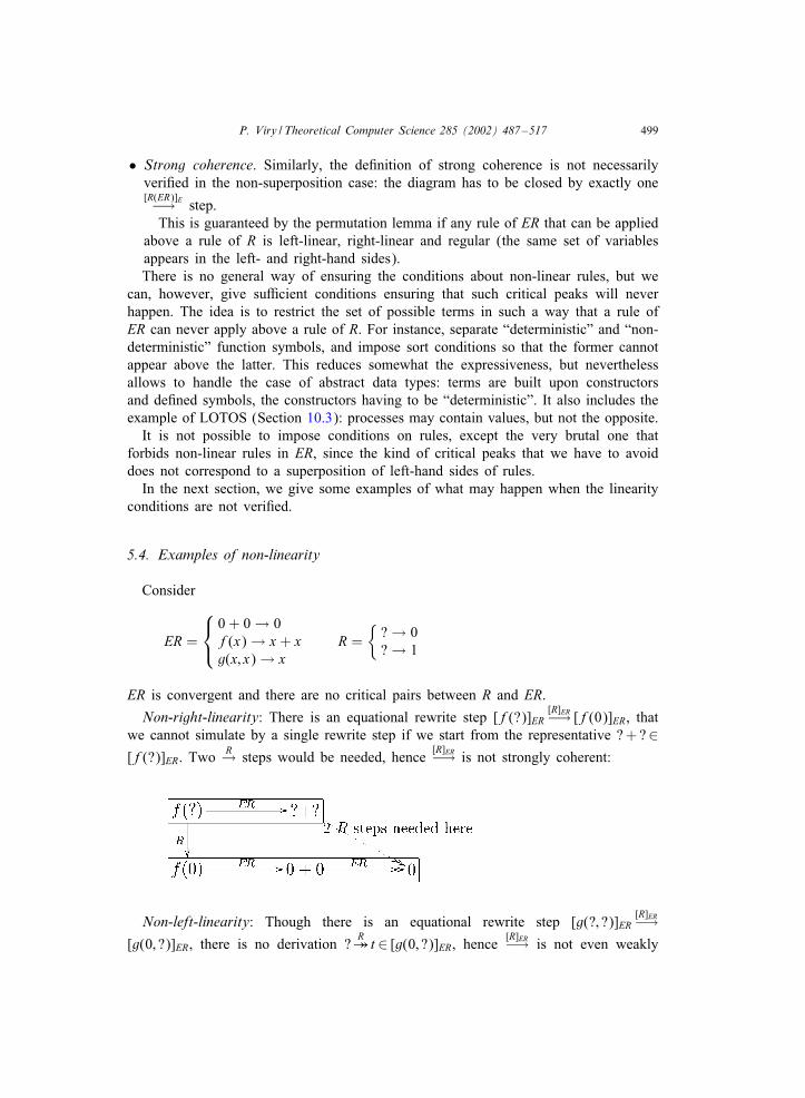
Consider
ER =
0 + 0→ 0f(x)→ x + xg(x; x)→ x
R ={?→ 0?→ 1
ER is convergent and there are no critical pairs between R and ER.
Non-right-linearity: There is an equational rewrite step [f(?)]ER[R]ER−→ [f(0)]ER, that
we cannot simulate by a single rewrite step if we start from the representative ?+ ?∈[f(?)]ER. Two
R→ steps would be needed, hence[R]ER−→ is not strongly coherent:
Non-left-linearity: Though there is an equational rewrite step [g(?; ?)]ER[R]ER−→
[g(0; ?)]ER, there is no derivation ?R� t ∈ [g(0; ?)]ER, hence [R]ER−→ is not even weakly
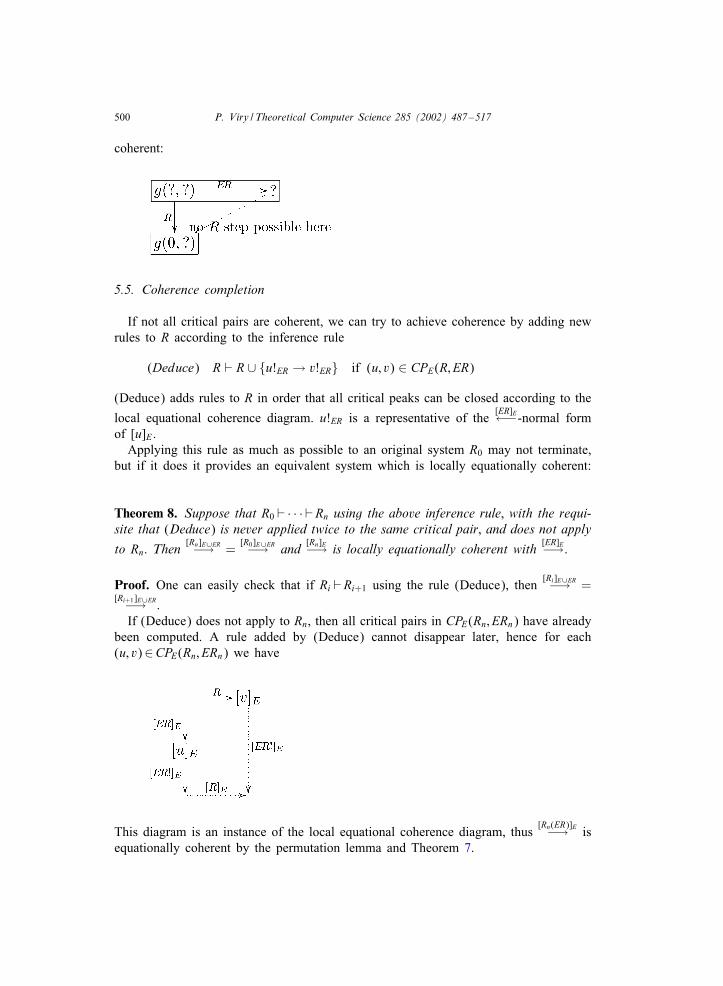
500 P. Viry / Theoretical Computer Science 285 (2002) 487–517
coherent:
5.5. Coherence completion
If not all critical pairs are coherent, we can try to achieve coherence by adding newrules to R according to the inference rule
(Deduce) R � R ∪ {u!ER → v!ER} if (u; v) ∈ CPE(R; ER)
(Deduce) adds rules to R in order that all critical peaks can be closed according to the
local equational coherence diagram. u!ER is a representative of the[ER]E←−-normal form
of [u]E .Applying this rule as much as possible to an original system R0 may not terminate,
but if it does it provides an equivalent system which is locally equationally coherent:
Theorem 8. Suppose that R0 � · · · �Rn using the above inference rule, with the requi-site that (Deduce) is never applied twice to the same critical pair, and does not apply
to Rn. Then[Rn]E∪ER−→ =
[R0]E∪ER−→ and[Rn]E−→ is locally equationally coherent with
[ER]E−→.
Proof. One can easily check that if Ri �Ri+1 using the rule (Deduce), then[Ri]E∪ER−→ =
[Ri+1]E∪ER−→ .If (Deduce) does not apply to Rn, then all critical pairs in CPE(Rn; ERn) have already
been computed. A rule added by (Deduce) cannot disappear later, hence for each(u; v)∈CPE(Rn; ERn) we have
This diagram is an instance of the local equational coherence diagram, thus[Rn(ER)]E−→ is
equationally coherent by the permutation lemma and Theorem 7.
P. Viry / Theoretical Computer Science 285 (2002) 487–517 501
For the cases of weak and strong coherence, the same completion procedure canbe used, but one still has to check separately that the conditions about critical peaksinvolving non-linear rules are veri9ed.This completion procedure is not related to the classical Knuth–Bendix completion
procedure. In particular:• Critical pairs are computed between two systems, not within one.• (Deduce) generates oriented rules, not equations.• The procedure does not rely on a given ordering, rather the orientation of the newrules is determined by the orientation of the rules already in R.
5.6. Completion modulo a rewrite system
In the particular case where R (in addition to ER) has an equational interpretation,there is a strong relationship between coherence completion and classical Knuth–Bendixcompletion:
Theorem 9. Remember that we always suppose[ER]E−→ con:uent. Suppose that
[R∪ER]E−→terminates. If
[R]E−→ is con:uent and[R(ER)]E−→ is equationally coherent; then
[R∪ER]E−→ iscon:uent.
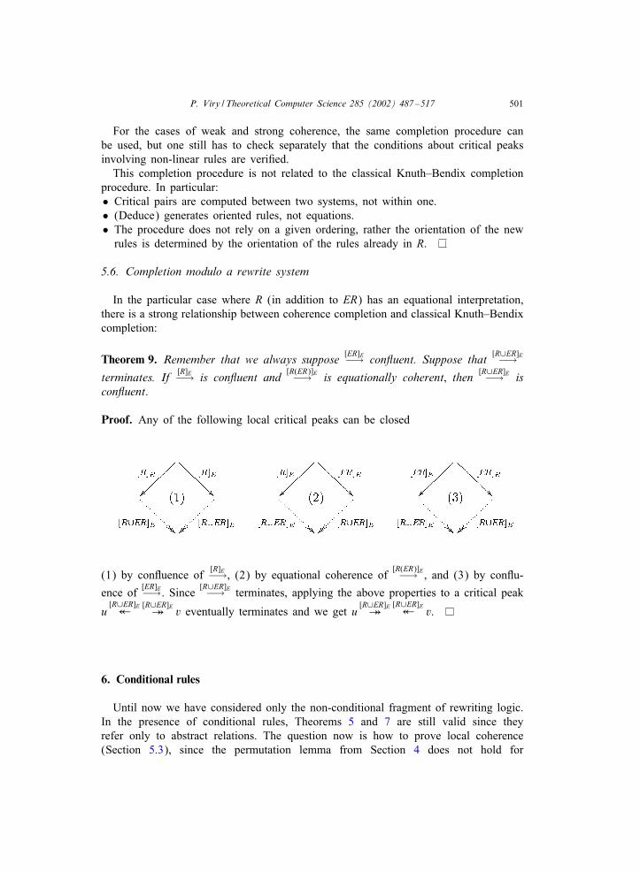
Proof. Any of the following local critical peaks can be closed
(1) by conBuence of[R]E−→, (2) by equational coherence of
[R(ER)]E−→ , and (3) by conBu-
ence of[ER]E−→. Since
[R∪ER]E−→ terminates, applying the above properties to a critical peak
u[R∪ER]E�
[R∪ER]E� v eventually terminates and we get u[R∪ER]E�
[R∪ER]E� v.
6. Conditional rules
Until now we have considered only the non-conditional fragment of rewriting logic.In the presence of conditional rules, Theorems 5 and 7 are still valid since theyrefer only to abstract relations. The question now is how to prove local coherence(Section 5.3), since the permutation lemma from Section 4 does not hold for
502 P. Viry / Theoretical Computer Science 285 (2002) 487–517
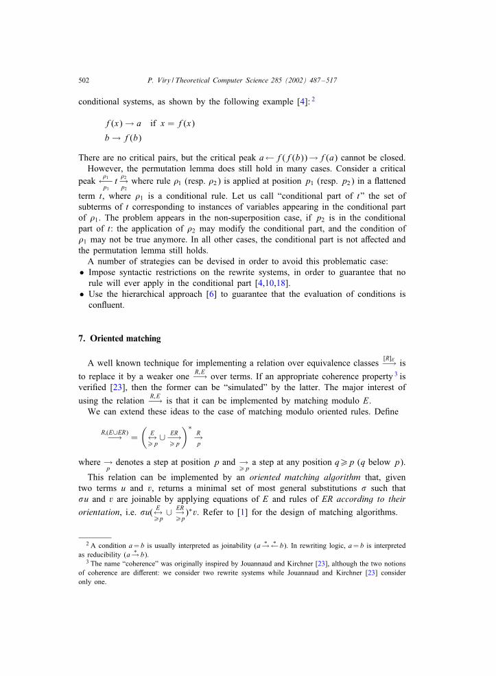
conditional systems, as shown by the following example [4]: 2
f(x)→ a if x = f(x)
b→ f(b)
There are no critical pairs, but the critical peak a←f(f(b))→f(a) cannot be closed.However, the permutation lemma does still hold in many cases. Consider a critical
peak�1←−p1
t�2→p2where rule �1 (resp. �2) is applied at position p1 (resp. p2) in a Battened
term t, where �1 is a conditional rule. Let us call “conditional part of t” the set ofsubterms of t corresponding to instances of variables appearing in the conditional partof �1. The problem appears in the non-superposition case, if p2 is in the conditionalpart of t: the application of �2 may modify the conditional part, and the condition of�1 may not be true anymore. In all other cases, the conditional part is not a;ected andthe permutation lemma still holds.A number of strategies can be devised in order to avoid this problematic case:• Impose syntactic restrictions on the rewrite systems, in order to guarantee that norule will ever apply in the conditional part [4,10,18].
• Use the hierarchical approach [6] to guarantee that the evaluation of conditions isconBuent.
7. Oriented matching
A well known technique for implementing a relation over equivalence classes[R]E−→ is
to replace it by a weaker oneR;E−→ over terms. If an appropriate coherence property 3 is
veri9ed [23], then the former can be “simulated” by the latter. The major interest of
using the relationR;E−→ is that it can be implemented by matching modulo E.
We can extend these ideas to the case of matching modulo oriented rules. De9ne
R;(E∪ER)−→ =(
E↔¿p∪ ER−→
¿p
)∗R→p
where →pdenotes a step at position p and →
¿pa step at any position q¿p (q below p).
This relation can be implemented by an oriented matching algorithm that, giventwo terms u and v, returns a minimal set of most general substitutions ! such that!u and v are joinable by applying equations of E and rules of ER according to theirorientation, i.e. !u( E↔
¿p∪ ER→¿p)∗v. Refer to [1] for the design of matching algorithms.
2 A condition a= b is usually interpreted as joinability (a ∗→ ∗← b). In rewriting logic, a= b is interpretedas reducibility (a ∗→ b).
3 The name “coherence” was originally inspired by Jouannaud and Kirchner [23], although the two notionsof coherence are di;erent: we consider two rewrite systems while Jouannaud and Kirchner [23] consideronly one.
P. Viry / Theoretical Computer Science 285 (2002) 487–517 503
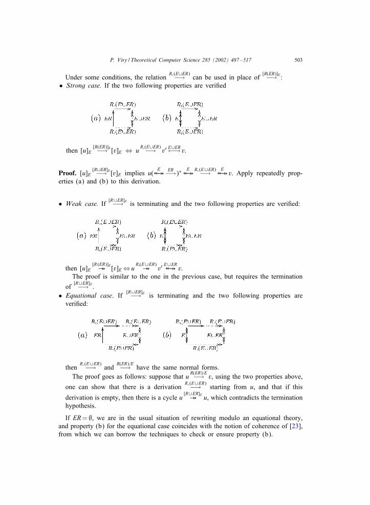
Under some conditions, the relationR; (E∪ER)−→ can be used in place of
[R(ER)]E−→ :• Strong case. If the two following properties are veri9ed
then [u]E[R(ER)]E−→ [v]E ⇔ u
R;(E∪ER)−→ v′ E∪ER←→ v:
Proof. [u]E[R∪ER]E−→ [v]E implies u(
E�� ER−→)∗ E
��R; (E∪ER)−→ E
�� v. Apply repeatedly prop-erties (a) and (b) to this derivation.
• Weak case. If[R∪ER]E−→ is terminating and the two following properties are veri9ed:
then [u]E[R (ER)]E� [v]E⇔ u
R;(E∪ER)� v′
E∪ER�� v.
The proof is similar to the one in the previous case, but requires the termination
of[R∪ER]E−→ .
• Equational case. If[R∪ER]E−→ is terminating and the two following properties are
veri9ed:
thenR; (E∪ER)−→ and
R(ER)=E−→ have the same normal forms.The proof goes as follows: suppose that u
R(ER)=E−→ v, using the two properties above,
one can show that there is a derivationR; (E∪ER)−→ starting from u, and that if this
derivation is empty, then there is a cycle u[R∪ER]E� u, which contradicts the termination
hypothesis.
If ER= ∅, we are in the usual situation of rewriting modulo an equational theory,and property (b) for the equational case coincides with the notion of coherence of [23],from which we can borrow the techniques to check or ensure property (b).
504 P. Viry / Theoretical Computer Science 285 (2002) 487–517
Property (a) is more unusual. Seemingly, checking it involves critical pairs betweena left-hand side of R and a right-hand side of ER. We can notice, however, that itholds in an important subcase, including identity and idempotency rules. Assume thatall right-hand sides of the rules in ER are variables, and consider a derivation
u ER→p
R;(E∪ER)→q
v ⇔ u ER→p
(E→¿q∪ ER→¿q
)∗R→qv
If p¿ q, then uR;(E∪ER)−→ v, since the 9rst ER step is below q, and property (a) is trivially
satis9ed. In all other cases, the two steps commute (since by hypothesis the rules inER have variables as right-hand sides), and property (a) is veri9ed for the weak andequational case. For the strong case, we also need to require that the variable formingthe right-hand side of a rule appears exactly once in its left-hand side.This technique extends to the case where only a subset of rules in ER have variable
right-hand sides, using the fact that if ER= S ∪T , then
[R(S∪T )]E→ ⇔ [R(S)(T (S))]E→
8. Rewriting modulo identity
As an example for equational coherence, we consider here the case of rewritingmodulo identity, famous for its termination problems. Consider R= {f(x+y)→f(x)+
f(y)} and E= {x + 0= x}. [R]E−→ does not terminate: we have
[f(x)]E[R]E→ [f(x) + f(0)]E
[R]E→ · · ·
since f(x)E��f(x + 0) R−→f(x) + f(0).
The problem here is that the equation x + 0= x can be used as expansion (fromright to left). Rewriting modulo identity would better be speci9ed as an oriented rule
x+0 =→ x in ER. In this case,[R(ER)]E−→ is not coherent, but coherence completion is able
to 9nd an equivalent strongly coherent system by adding a rule to R:
ER = {x + 0 =→ x}; R =
{f(x + y)→ f(x) + f(y)
f(x)→ f(x) + f(0)
}
Note that the orientation of the rule f(x)−→f(x) + f(0) is 9xed by the completionprocedure.
[R(ER)]E−→ is still non-terminating, but one cannot blame coherence (or identity) com-
pletion: since completion tries to simulate the relation[R]E∪ER−→ , which does not terminate,
one cannot expect to get a terminating relation. However, there is a solution if we areonly interested in equational coherence. Suppose that R contains additional rules for f,
P. Viry / Theoretical Computer Science 285 (2002) 487–517 505
for instance:
ER = {x + 0 =→ x}; R =
{f(x + y) → f(x) + f(y)
f(0) → 0
}
Then[R(ER)]E−→ is equationally coherent, and
[R(ER)]E−→ is terminating even though[R]E∪ER−→
is not, basically because equational coherence does not require that we simulate theidentity step
[f(x)]ER[R]ER→ [f(x)]ER
Of course, it would be impossible to get a terminating relation if we demand strongcoherence (weak coherence is possible by adding rules to ER instead of R).
9. Calculi with bound variables
Bound variables appear in many di;erent calculi. In the �-calculus, they are higher-order variables, bound by �. In the �-calculus, they are channel names bound by *and Sx. Other examples of variable binders are the logical quanti9ers ∀ and ∃, or theintegration operator. In all these calculi, terms are taken up to the renaming of boundvariables (+-conversion), and substitution is considered as a meta-theoretic operator.Trying to describe such calculi in a 9rst-order setting, bound variables become just
names, and substitution has to be made explicit as a 9rst-order operator. Bound vari-ables are usually replaced by De Bruijn indices in order to “build-in” +-conversion.We end up with two di;erent notions of variables and substitutions, however usuallyonly ground terms (not containing 9rst-order variables) are considered. First-order vari-ables may be introduced for solving equations (e.g. higher-order uni9cation [12]), withrestrictions over where they may appear.The explicit substitution approach has the advantage of modelling very precisely the
possible implementations of a calculus. It is shown in [20] how di;erent strategies forthe application of substitution rules of the weak �!-calculus correspond to di;erentmodels of machines implementing this calculus, and moreover that a machine can bederived quite easily from a given strategy.Many substitution calculi have been proposed, with various conBuence, termination
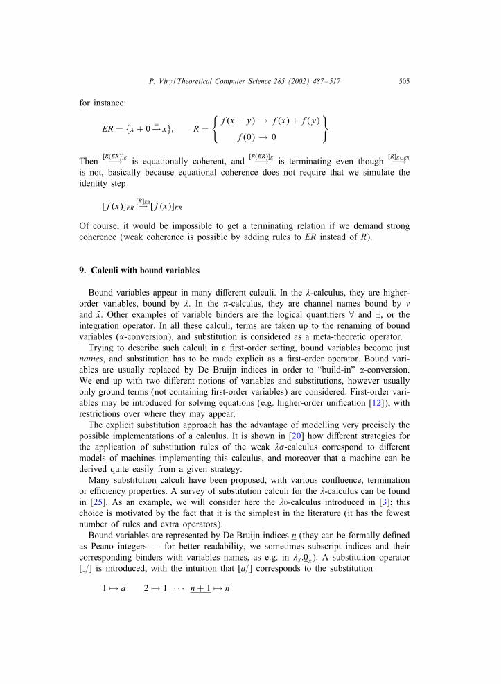
or eHciency properties. A survey of substitution calculi for the �-calculus can be foundin [25]. As an example, we will consider here the �,-calculus introduced in [3]; thischoice is motivated by the fact that it is the simplest in the literature (it has the fewestnumber of rules and extra operators).Bound variables are represented by De Bruijn indices n (they can be formally de9ned
as Peano integers — for better readability, we sometimes subscript indices and theircorresponding binders with variables names, as e.g. in �x:0x). A substitution operator[ =] is introduced, with the intuition that [a=] corresponds to the substitution
1 �→ a 2 �→ 1 · · · n+ 1 �→ n
506 P. Viry / Theoretical Computer Science 285 (2002) 487–517
�-reduction is simulated by the only reduction rule
R = {(�a)b→ a[b=]}Note that the fact of putting �-reduction as a rule of R does not imply that it cannotbe equationally interpreted. If it is, then the partitioning of rules between R and ERis still useful as a hierarchical composition mechanism. At the lower level, one willsee all the implementation details including the application of substitutions, while theywill be hidden at the upper level.The equational rules specify how to reduce terms containing substitutions (two aux-
iliary operators ↑ and ⇑ are introduced):
ER =
(ab)[s] =→ a[s]b[s](�a)s =→ �(a[⇑ (s)])1[a=] =→ an+ 1[a=] =→ n
1[⇑ (s)] =→ 1n+ 1[⇑ (s)] =→ n[s][↑]n[↑] =→ n+ 1
It is shown in [3] that
• The �,-calculus is a conservative extension of the �-calculus: the relation R−→ ER!�
over pure terms (not containing [ =], ↑ or ⇑ ( )) coincides with �-reduction, hence
alsoR(ER!)−→ (putting aside the last
ER!� steps of a derivation).
• ER−→ is convergent.• R∪ER−→ is conBuent over ground terms. This cannot be shown by the usual critical pairanalysis, because there is a non-conBuent critical pair between the rule in R and the9rst rule of ER.If conBuence over open terms is required, the system �!⇑ from [19] can be used,
it is, however, much more complex than our example.
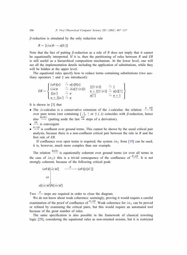
The relationR(ER)−→ is equationally coherent over ground terms (or over all terms in
the case of �!⇑): this is a trivial consequence of the conBuence of R∪ER−→ . It is notstrongly coherent, because of the following critical peak:
(ab)[(�c)d] R−−−−−→ (ab)[c[d=]]
ER
�a[(�c)d]b[(�c)d]
Two R−→ steps are required in order to close the diagram.We do not know about weak coherence: seemingly, proving it would require a careful
examination of the proof of conBuence of R∪ER−→ . Weak coherence for �!⇑ can be provedor refuted by examining the critical pairs, but this would require an automated toolbecause of the great number of rules.The same speci9cation is also possible in the framework of classical rewriting
logic [29], considering the equational rules as non-oriented axioms, but it is restricted
P. Viry / Theoretical Computer Science 285 (2002) 487–517 507
to a semantic description since rewriting modulo such a complex theory is not prac-tically feasible. The fact of having two sets of rules is useful for relating �-reductionand its implementation in a single framework.
10. Process algebras
In this second example, we will develop the case of the �-calculus augmented withabstract data types.The �-calculus [34] and LOTOS [5] are two modern representatives of the process
algebra tradition that emerged from earlier works on CSP [21] and CCS [34]. The�-calculus describes mobile processes, where mobility is achieved by the introductionof binder operators and bound variables allowing name passing.LOTOS integrates processes and data types in a two-level framework. The 9rst is
based on CSP=CCS, the second is based on ACT-ONE, a speci9cation language forabstract data types. This layer structure is not completely satisfactory, as noticed in anintroductory book [34, p. 70]:
(...) many elements of a system can be speci9ed both as processes and as datatypes. (...) a deeper understanding of the relation between the two componentscould be bene9cial, and some harmonization between them could be attempted(...), for instance a common semantic model.
We will see here how an oriented rewrite theory provides such a common semanticmodel.
10.1. Structure of �-calculus processes
As in the previous section, the bound variables of the �-calculus will be representedby indices and the substitution operation will be made explicit using the substitutioncalculus part of �, (i.e. without �-reduction).The terms of the �-calculus with indices are de9ned as follows (using a syntax more
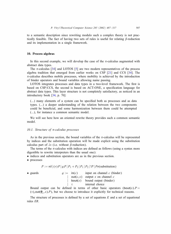
digestible to rewrite interpreters than the usual one):• indices and substitution operators are as in the previous section.• processes
P := nil | (*)P | g:P |P1 + P2 |P1 |P2 | !P |P!(substitution)• guards g := in(c) input on channel c (binder)
| out(c; x) output x on channel c| bout(x) bound output (binder)| - internal choice
Bound output can be de9ned in terms of other basic operators (bout(x):P=(*)cout(0 c; x):P), but we choose to introduce it explicitly for technical reasons.
The structure of processes is de9ned by a set of equations E and a set of equationalrules ER.
508 P. Viry / Theoretical Computer Science 285 (2002) 487–517
Processes are considered modulo the equations AC(+) and AC(|) (associativity andcommutativity of the + and | operators) and the following equational rules:
P + nil =→ PP | nil =→ P
P | (*)Q =→ (*) ([↑]P |Q)The substitution rules of �, from the previous section are also part of the equationalrules.The last two equational rules allow to replace | and ! operators with non-deterministic
choice:The expansion rule: Let P= +1:P1 + · · · ++n:Pn and Q= �1:Q1 + · · · +�m:Qm, then
P |Q =−→ ∑i=1:::n
+i:(Pi |Q) +∑
i=1:::m�i:(P |Qi) +
∑i=1:::nj=1:::m
Sync(+i:Pi; �j:Qj)
where
Sync(+i:Pi; �j:Qj) =
-:(Pi[z=]|Qj) if +i = in(x) and �j = out(x; z)
-:(*)(Pi|Qj) if +i = in(x) and �j = bout(x)
(and similarly by swapping the arguments)
nil in all other cases
The replication rule: Let P= g1:P1 + · · ·+ gn:Pn, then
!P =→ g1:(P1|!P) + · · ·+ gn:(Pn|!P)A process is in weak disjunctive normal form [34] if it is of the form
(*) : : : (*)(g1:P1 + · · ·+ gn:Pn)
with n¿0. Using the above equational rules, any process can be put in weak disjunctivenormal form.Expansion and replication are rule schemes rather than proper rewrite rules because
of the variable n, but can be easily simulated using extra hidden operators.The rewrite relation de9ned by the above equational rules (modulo AC) does not
terminate because of the replication rule that can be applied repeatedly into its ownright-hand side. In order to ensure termination, the rewrite rules must be appliedaccording to a strategy $ that allows application of the replication rule only whenneeded in order to compute a weak disjunctive normal form.
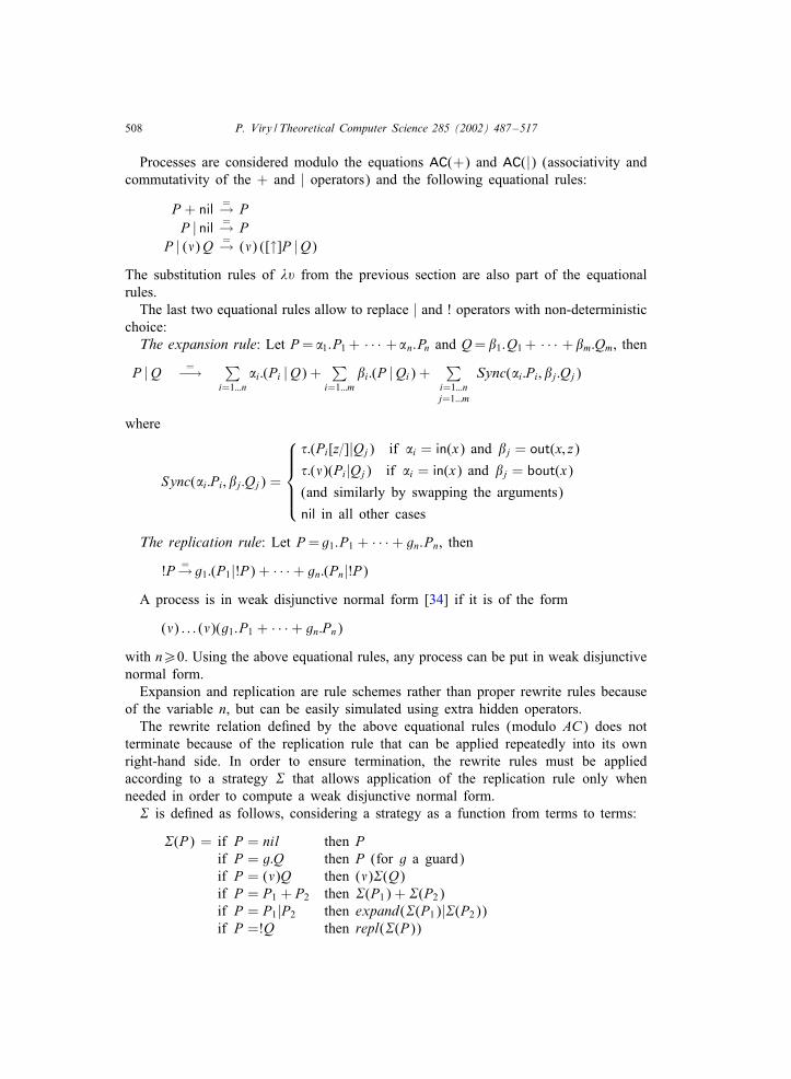
$ is de9ned as follows, considering a strategy as a function from terms to terms:
$(P) = if P = nil then Pif P = g:Q then P (for g a guard)if P = (*)Q then (*)$(Q)if P = P1 + P2 then $(P1) + $(P2)if P = P1|P2 then expand($(P1)|$(P2))if P =!Q then repl($(P))
P. Viry / Theoretical Computer Science 285 (2002) 487–517 509
where expand(P) applies the expansion theorem at the top of P and repl(P) thereplication theorem. The remaining rules are applied freely. A simple induction showsthat expand and repl are always applied to arguments where the corresponding rulecan be applied, and the maximal number of application of $ is bounded by the sizeof the input term.
Let us denote[ER]E�→ the derivations using all the above equational rules according to
this strategy $, then we have the following correspondence result:
Proposition 10 (Viry [41]). There is a one-to-one correspondence between processesof the original �-calculus (modulo the usual structural axioms) and normal forms
with respect to[ER]E�→ .
Proof.• By construction, there is a one-to-one correspondence between processes of theoriginal �-calculus (modulo the usual structural axioms) and equivalence classesmodulo ER∪E.
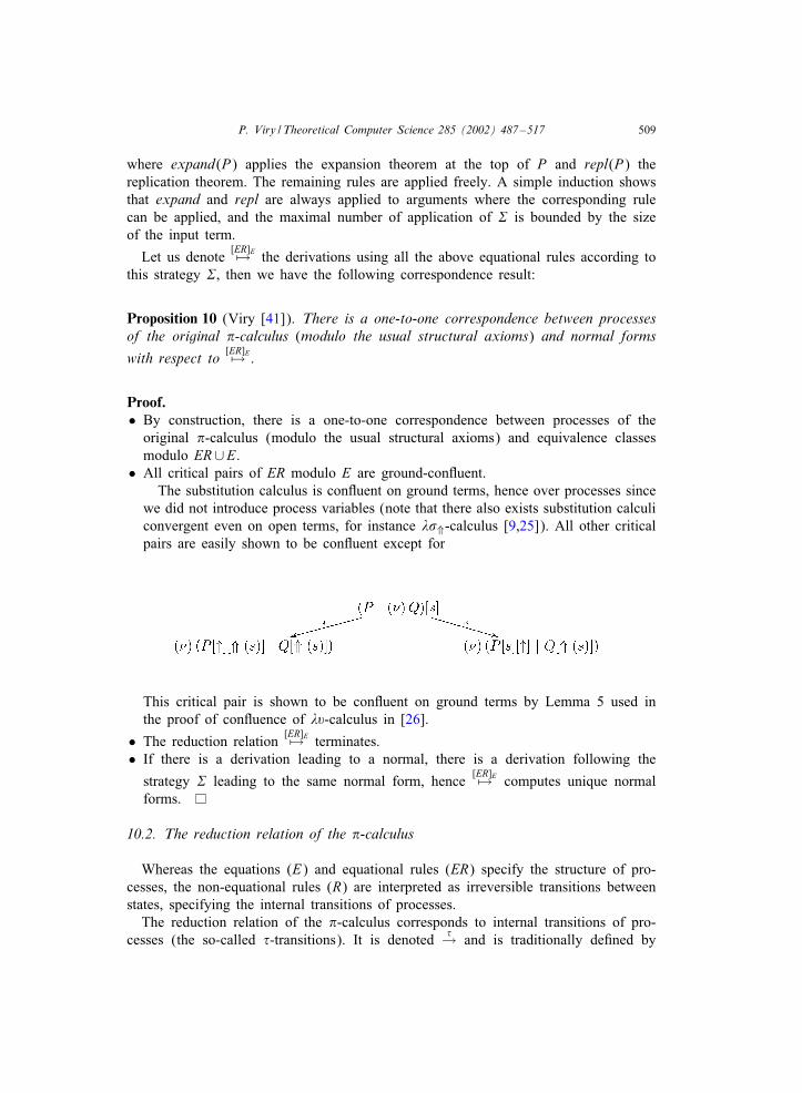
• All critical pairs of ER modulo E are ground-conBuent.The substitution calculus is conBuent on ground terms, hence over processes since
we did not introduce process variables (note that there also exists substitution calculiconvergent even on open terms, for instance �!⇑-calculus [9,25]). All other criticalpairs are easily shown to be conBuent except for
This critical pair is shown to be conBuent on ground terms by Lemma 5 used inthe proof of conBuence of �,-calculus in [26].
• The reduction relation [ER]E�→ terminates.• If there is a derivation leading to a normal, there is a derivation following the
strategy $ leading to the same normal form, hence[ER]E�→ computes unique normal
forms.
10.2. The reduction relation of the �-calculus
Whereas the equations (E) and equational rules (ER) specify the structure of pro-cesses, the non-equational rules (R) are interpreted as irreversible transitions betweenstates, specifying the internal transitions of processes.The reduction relation of the �-calculus corresponds to internal transitions of pro-
cesses (the so-called --transitions). It is denoted -→ and is traditionally de9ned by
510 P. Viry / Theoretical Computer Science 285 (2002) 487–517
the following inference rules [22]:
-:P + Q -→ (Choice)P -→P′
P|Q -→P′|QP -→P′
(*)P -→(*)P′
If we want to consider (Choice) as a rewrite rule, we have to make sure that it can beapplied only under the allowable contexts. Such a strategy can be easily implementedby 9rst reducing processes with the equational rules, since we know the shape of weakdisjunctive normal forms.We will thus consider (Choice) as the only non-equational rule in R. Its application
according to the above strategy will be denoted[R]E�→ . The correspondence result is as
follows:
Proposition 11 (Viry [41]). There is a reduction step P -→Q in the original �-calculus
if and only if there is a rewrite derivation [P]E[ER]E�→ [R]E�→ [Q′]E , where [Q′]
[ER]E�� Q.
This result is proved by showing strong coherence between equational and reductionrules (note that (Choice) is a linear rule). Although the rules in our speci9cation mustbe applied according to some speci9c strategies, Theorems 5 and 7 are still valid sincethey refer only to abstract relations. As for the proof of local coherence, one has toensure that the strategies are preserved by the permutation lemma, and that the localcoherence diagram can be closed according to these strategies.
We have implemented the relation[ER]E�→ [R]E�→ in ELAN [24], which o;ers a power-
ful strategy speci9cation mechanism and a eHcient AC-rewriting engine (we believethat our speci9cation would be very diHcult to encode using the OBJ [17] strategymechanism).With the addition of a few new built-in operators, we have been able to design
an eHcient and semantically clean input–output system for ELAN based on this rela-tion [41].
10.3. Addition of data types
So far, we have considered the plain monadic �-calculus. As shown in [34], thiscalculus is powerful enough to encode any kind of structured data, so the game mayend here. However, for practical purposes one would like to be able to de9ne the dataexchanged by processes using abstract data types (ADTs).ADTs are straightforwardly encoded with equational rules, but we have to guarantee
coherence in order for the above correctness results to still hold. As long as the op-erators of the ADTs are disjoint from those of the �-calculus, this does not introducenew critical pairs, and if we impose that data types appear only within processes, asin LOTOS, then the linearity conditions are trivially veri9ed.
P. Viry / Theoretical Computer Science 285 (2002) 487–517 511
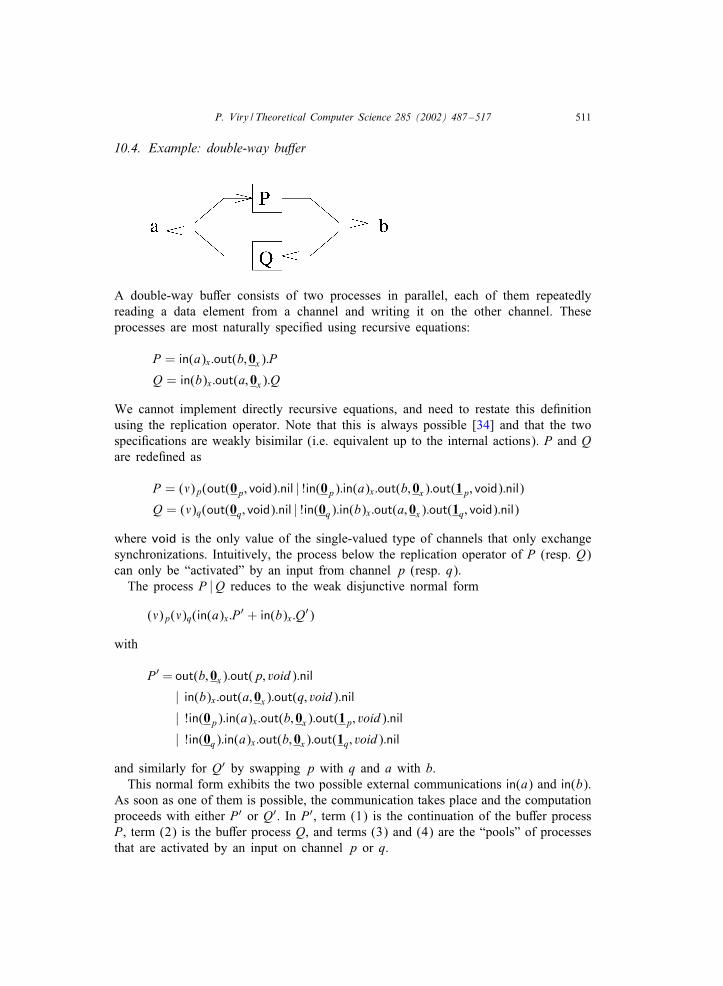
10.4. Example: double-way bu>er
A double-way bu;er consists of two processes in parallel, each of them repeatedlyreading a data element from a channel and writing it on the other channel. Theseprocesses are most naturally speci9ed using recursive equations:
P = in(a)x:out(b; 0x):P
Q = in(b)x:out(a; 0x):Q
We cannot implement directly recursive equations, and need to restate this de9nitionusing the replication operator. Note that this is always possible [34] and that the twospeci9cations are weakly bisimilar (i.e. equivalent up to the internal actions). P and Qare rede9ned as
P = (*)p(out(0p; void):nil | !in(0p):in(a)x:out(b; 0x):out(1p; void):nil)
Q = (*)q(out(0q; void):nil | !in(0q):in(b)x:out(a; 0x):out(1q; void):nil)
where void is the only value of the single-valued type of channels that only exchangesynchronizations. Intuitively, the process below the replication operator of P (resp. Q)can only be “activated” by an input from channel p (resp. q).The process P |Q reduces to the weak disjunctive normal form
(*)p(*)q(in(a)x:P′ + in(b)x:Q′)
with
P′ = out(b; 0x):out(p; void):nil
| in(b)x:out(a; 0x):out(q; void):nil
| !in(0p):in(a)x:out(b; 0x):out(1p; void):nil
| !in(0q):in(a)x:out(b; 0x):out(1q; void):nil
and similarly for Q′ by swapping p with q and a with b.This normal form exhibits the two possible external communications in(a) and in(b).
As soon as one of them is possible, the communication takes place and the computationproceeds with either P′ or Q′. In P′, term (1) is the continuation of the bu;er processP, term (2) is the bu;er process Q, and terms (3) and (4) are the “pools” of processesthat are activated by an input on channel p or q.
512 P. Viry / Theoretical Computer Science 285 (2002) 487–517
So far we remained within the framework of the �-calculus. As an example of theaddition of ADTs, the two-way bu;er example can be extended by adding computationof the output values, for instance
P = in(a)x:out(b; f(0x)):P
Q = in(b)x:out(a; g(0x)):P
where f and g are functions de9ned by equational rules. Since these de9ned operatorsappear only strictly below process operators, we are guaranteed that strong coherenceis preserved and thus that our implementation remains correct.
10.5. Example: ?lter
In the previous example, in order to enforce the non-linearity conditions for strongcoherence, data types appear only below processes. Actually, the non-linearity condi-tions are veri9ed as well if process expressions appear below de9ned symbols, as longas no non-linear rewrite rule may ever be applied above a process expression.This is the case for instance with the if:::then:::else::: operator, de9ned by the fol-
lowing linear rules
if true then x else y → x
if false then x else y → y
Then we can write a FILTER process, that repeatedly inputs values on a channel iand copies them on an output channel o only when they verify a given condition:
FILTER = in(i)x: if c(x) then out(o; 0x):FILTER else FILTER
This recursive de9nition is then restated using the replication operator as in the previousexample.This possibility allows for a much more “natural” programming style, similar to
CSP=Occam [21], but the constructs that may appear above processes must be clearlyidenti9ed in order to ensure the condition about non-linear rules.
11. Sequent calculus modulo
Our third and last example concerns the case where the rewrite relation is interpretedas deduction steps.
11.1. An oriented rewriting logic theory for the sequent calculus
The sequent calculus is a quite complex logical system which has been thoroughlystudied in the literature. Our motivation for choosing to study this particular calculusis to show a non-trivial example; other than that, this choice is purely arbitrary, and inparticular we will not develop logical considerations but will rather remain on a purelysyntactic level.
P. Viry / Theoretical Computer Science 285 (2002) 487–517 513
R ={
Axiom A; C � C; B → ✸
L∀ A;∀3:C � B → A; C[a=3] � B
ER = $∪
L∨ A; C ∨ D � B =→ A; C � B • A;D � BR∧ A � C ∧ D; B =→ A � C; B • A � D; BR∀ A�∀3:C; B =→ A�C; B
Uc A; =→ AU• A •✸ =→ A
f¬ ¬¬A =→ Af⇒ A⇒ B =→ ¬A ∨ B
U∨ A ∨ 0 =→ AU∧ A ∧ 1 =→ A
Z∨ A ∨ ¬A =→ 1Z∧ A ∧ ¬A =→ 0
fI ∧ A∧A =→ AfI∨ A ∨ A =→ A
f∀ ∀x:A =→ ¬∃x:¬A
sIl A; C; C �B =→ A; C �BsIr A�C; C; B =→ A�C; Bs¬l A; C �B =→ A�¬C; Bs∧ A; C ∧D�B =→ A; C; D�Bs∨ A�C ∨ D; B =→ A�C;D; B
E =
Ac A; (B; C) = (A; B); CCc A; B = B; A
A• A • (B • C) = (A • B) • CC• A • B = B • A
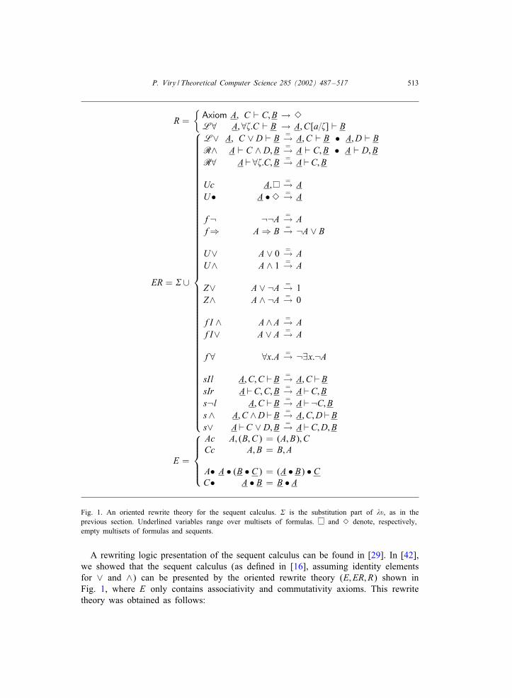
Fig. 1. An oriented rewrite theory for the sequent calculus. $ is the substitution part of �,, as in theprevious section. Underlined variables range over multisets of formulas. and ✸ denote, respectively,empty multisets of formulas and sequents.
A rewriting logic presentation of the sequent calculus can be found in [29]. In [42],we showed that the sequent calculus (as de9ned in [16], assuming identity elementsfor ∨ and ∧) can be presented by the oriented rewrite theory (E; ER; R) shown inFig. 1, where E only contains associativity and commutativity axioms. This rewritetheory was obtained as follows:
514 P. Viry / Theoretical Computer Science 285 (2002) 487–517
• Put in E the equations making explicit the implicit structure of formula and sequentcomposition (such as associativity and commutativity) together with the equationsde9ning the explicit substitution calculus. Turn all inference rules of the originalsequent calculus de9nition into R rules:
premissesconsequences
becomes consequences → premisses
A proof of a sequent 7 is thus encoded into a rewriting logic sentence + :7→ ✸,
corresponding to a rewrite derivation [7]E[R]E� [✸]E .
• Then, add to E equational consequences of this system, such as idempotency offormula composition. This allows in turn to simplify the presentation by removingrules in R that have become redundant.• Finally, turn selected equations of E and selected rules of R into equational rulesin ER. This selection (and the orientation given to equations) is rather arbitrary: theonly requirement is that the resulting oriented rewrite theory be weakly coherent,and one also usually wishes to keep in E only axioms for A and AC symbols.A di;erent selection or a di;erent orientation of equations would provide a dif-
ferent view of sequent calculus proofs. For instance, moving a rule from R to ERcorresponds to what is usually called “building-in equality” in theorem provers [7].Building-in equality can make proofs much smaller, at the expense of hiding logicaldetails.
The main result of [42] states that:
Proposition 12. The sequent 7 is provable in the sequent calculus if and only if there
is a rewrite derivation [7]E[R(ER)]E� [�]E .
Proof.• By construction, and using two lemmas stating that adding equational consequencesand removing redundant rules preserves derivability, we have that the sequent 7is provable in the sequent calculus if and only if there is a rewrite derivation
[7]E∪ER[R]E∪ER� [�]E∪ER (where � denotes the empty sequent multiset).
• ER−→ is convergent and[R(ER)]E−→ is weakly coherent.
All critical pairs of ER are conBuent and termination is shown using an AC-compatible recursive path ordering [2].Weak coherence is shown by examining critical pairs. Since we reduce multisets
of sequents, and rules of R only apply at the “sequent level”, the situation where anon-left linear rule of ER is applied above a rule of R cannot happen.
11.2. Theorem proving modulo
Now, we can think of adding additional equations or equational rules modulo whichwe wish to do reasoning. These equations may for instance de9ne new operators orspecify the internal structure of the objects we reason about. By doing so, we end upwith a framework similar to that of “theorem proving modulo” introduced in [13].
P. Viry / Theoretical Computer Science 285 (2002) 487–517 515
As long as weak coherence is still veri9ed, new equations and equational rules can beadded, while preserving the correctness of the implementation. Because the additionalequations one may wish to introduce most often involve only new symbols not presentin the original calculus, weak coherence is trivially preserved (no new critical pairs are
introduced), and termination of[ER]E−→ may be proved using modularity results [36,15].
In this way, we can handle the example of higher-order logic given in [13]. Theformulas of the sequent calculus are extended with a few operators, and consideredmodulo equations. Intuitively, the operators ¬̇, ∨̇ and ∀̇ are external versions of theirsequent calculus counterparts, + denotes application, and 8 maps the external versionof a term to its internal version. The three equations giving the speci9cation of 8 arebetter expressed as equational rules:
8(+(¬̇; x)) =−→¬8(x)
8(+(+(∨̇; x); y)) =−→ 8(x) ∨ 8(y)
8(+(∀̇T ; x)) =−→∀y:8(+(x; y))
Then it is possible to show that ER augmented with these rules is still convergent andthat weak coherence is preserved, hence we immediately obtain a correct implementa-tion of this extended sequent calculus modulo equations.
12. Conclusion
The introduction of equational rules solves the dilemma, inherent to rewriting logic,of whether to specify something as a rule or as an equation. Turning equations intoequational rules can lead to better eHciency (some rules can even be internalized intoan oriented matching algorithm), while turning rules into equational rules can be seenas “building-in” equality. Equational rules can also serve as a way of hierarchicallystructuring systems.When using equational rules, one must ensure that their operational behavior corre-
sponds to their intended meaning. We proposed various suHcient conditions (variousnotions of coherence) and veri9cation techniques based on critical pair criteria.The three examples developed in the paper cover the most important interpretations
of rewriting logic (transitions, deductions and equality), and should provide a templatefor most applications. In each case, we obtained an oriented rewrite theory containingonly the associativity and commutativity axioms, which can be easily implemented onusual rewriting interpreters or compilers.Rewriting logic as a logical framework o;ers a natural and simple way of specifying
most calculi encountered in practice, but the lack of equational rules makes its imple-mentation diHcult. We believe that by solving this behavior vs. semantics dilemma,we removed one of the most important barriers in the way of a wide practical use ofrewriting logic.
516 P. Viry / Theoretical Computer Science 285 (2002) 487–517
Acknowledgements
My thanks go to the anonymous referees who provided many constructive comments.
References
[1] M. Adi, C. Kirchner, AC-uni9cation race: the system solving approach, implementation and benchmarks,J. Symbolic Comput. 14 (1) (1992) 51–70.
[2] F. Baader, T. Nipkow, Term Rewriting and All That, Cambridge University Press, Cambridge, 1999.[3] Z. Benaissa, D. Briaud, P. Lescanne, J. Rouyer-Degli, �,, a calculus of explicit substitutions which
preserves strong normalisation, Technical Report 2477, INRIA, February 1995.[4] J.A. Bergstra, J.W. Klop, Conditional rewrite rules: conBuency and termination, J. Comput. System Sci.
32 (3) (1986) 323–362.[5] T. Bolognesi, E. Brinksma, Introduction to the ISO speci9cation language LOTOS. in: P.H.J. van Eijk,
C.A. Vissers, M. Diaz (Eds.), The Formal Description Technique LOTOS, Elsevier Science PublishersB.V., North-Holland, 1989, pp. 23–73.
[6] W. Bousdira, J.-L. RVemy, Hierarchical contextual rewriting with several levels, in: R. Cori, M. Wirsing(Eds.), 5th Ann. Symp. on Theoretical Aspects of Computer Science, Bordeaux, France, Lecture Notesin Computer Science, Vol. 294, Springer, Berlin, 1988, pp. 193–206.
[7] S. Boutin, Using reBection to build eHcient and certi9ed decision procedures, in: M. Abadi, T. Ito(Eds.), TACS’97, Lecture Notes in Computer Science, Vol. 1281, Springer, Berlin, 1997.
[8] H. Comon, J.-P. Jouannaud, Uni9cation and disuni9cation in shallow theories, in: H. Comon (Ed.),Proc. 5th Internat. Workshop on Uni9cation, Barbizon, France, 1991.
[9] P.-L. Curien, Th. Hardin, J.-J. LVevy, ConBuence properties of weak and strong calculi of explicitsubstitutions, RR 1617, INRIA, Rocquencourt, February 1992.
[10] N. Dershowitz, M. Okada, G. Sivakumar, ConBuence of conditional rewrite systems, in: J.-P. Jouannaud,S. Kaplan (Eds.), Proc. 1st Internat. Workshop on Conditional Term Rewriting Systems, Orsay, France,Lecture Notes in Computer Science, Vol. 308, Springer, Berlin, July 1987, pp. 31–44.
[11] E. Domenjoud, Outils pour la dVeduction automatique dans les thVeories associatives–commutatives, ThXesede Doctorat d’UniversitVe, UniversitVe de Nancy 1, September 1991.
[12] G. Dowek, Th. Hardin, C. Kirchner, Higher-order uni9cation via explicit substitutions, in: D. Lugiez(Ed.), Proc. 8th Internat. Workshop on Uni9cation, Val d’Ajol, France, CRIN, June, 1994.
[13] G. Dowek, Th. Hardin, C. Kirchner, Theorem proving modulo, Technical Report 3400, INRIA, 1998.[14] F. DurVan, Coherence checker and completion tools for maude speci9cations, Technical report,
Dpto. de Lenguajes y Ciencias de la Computation, Universidad de MValaga, 2000, Available fromhttp:==maude.csl.sri.com=papers=coherence.
[15] M. Fernandez, J.-P. Jouannaud, Modular termination of term rewriting systems revisited, in: Proc. of11th Workshop on Speci9cation of Abstract Data Types, Lecture Notes in Computer Science, Vol. 906,Springer, Berlin, 1995.
[16] J.-Y. Girard, Y. Lafont, P. Taylor, Proofs and types, Cambridge Tracts in Theoretical Computer Science,Vol. 7, Cambridge University Press, Cambridge, 1989.
[17] J.A. Goguen, T. Winkler, J. Meseguer, K. Futatsugi, J.-P. Jouannaud, Introducing OBJ, in: J.A.Goguen, G. Malcolm (Eds.), Software Engineering with OBJ: Algebraic Speci9cation in Action, KluwerAcademic Publishers, Dordrecht, 2000, pp. 3–167.
[18] B. Gramlich, On termination and conBuence of conditional rewrite systems, in: Proc. 4th Internat.Workshop on Conditional and Typed Rewriting Systems (CTRS’94), Jerusalem, Lecture Notes inComputer Science, Vol. 968, Springer, Berlin, 1994.
[19] Th. Hardin, J.-J. LVevy, A conBuent calculus of substitutions, in: France–Japan Arti9cial Intelligence andComputer Science Symposium, Izu, 1989.
[20] T. Hardin, L. Maranget, B. Pagano, Functional Back-Ends within the Lambda-Sigma Calculus.Proceedings of ICFP 1996, Philadelphia, Pennsylvania, May 24–26, 1996, SIGPLAN Notices 31(6),June 1996, ACM Press, ISBN 0-89791-770-7.
P. Viry / Theoretical Computer Science 285 (2002) 487–517 517
[21] C.A.R. Hoare, Communicating sequential processes, Commun. ACM 21 (8) (1978) 666–677.[22] K. Honda, N. Yoshida, On reduction-based process semantics, in: Proc. of 13th Conference on
Foundations of Software Technology and Theoretical Computer Science, Lecture Notes in ComputerScience, Vol. 761, Springer, Berlin, 1993, pp. 371–387.
[23] J.-P. Jouannaud, H. Kirchner, Completion of a set of rules modulo a set of equations, SIAM J.Comput. 15(4) (1986) 1155–1194, Preliminary version in Proc. 11th ACM Symposium on Principlesof Programming Languages, Salt Lake City, USA, 1984.
[24] C. Kirchner, H. Kirchner, M. Vittek, Designing constraint programming languages using computationalsystems, in: P. Van Hentenryck, S. Saraswat (Eds.), Principles and Practice of Constraint Programming,The MIT Press, Cambridge, MA, 1995.
[25] P. Lescanne, From �! to �,, a journey through calculi of explicit substitutions, in: Hans Boehm (Ed.),Proc. of the 21st Annual ACM Symposium on Principles of Programming Languages, Portland, OR,USA, ACM, 1994, pp. 60–69.
[26] P. Lescanne, J. Rouyer-Degli, The calculus of explicit substitutions �,, Technical Report RR-2222,INRIA-Lorraine, January 1994.
[27] C. MarchVe, RVeVecriture modulo une thVeorie prVesentVee par un systXeme convergent et dVecidabilitVe duproblXeme du mot dans certaines classes de thVeories Vequationnelles, ThXese de Doctorat d’UniversitVe,UniversitVe de Paris-Sud, Orsay, France, October 1993.
[28] C. MarchVe, Normalised rewriting and normalised completion, in: Proc. 9th Symp. on Logic in ComputerScience, IEEE Computer Society Press, Silverspring, MD, 1994, pp. 394–403.
[29] N. MartVZ-Oliet, J. Meseguer, Rewriting logic as a logical and semantic framework, Technical reportCSL-93-05, SRI International, 1993.
[30] The Maude system, http:==maude.csl.sri.com.[31] J. Meseguer, Conditional rewriting logic as a uni9ed model of concurrency, Theoret. Comput. Sci.
96 (1) (1992) 73–155.[32] J. Meseguer, A logical theory of concurrent objects and its realisation in the Maude language, in:
G. Agha, P. Wegner, A. Yonezawa (Eds.), Research Directions in Object-Based Concurrency, The MITPress, Cambridge, MA, 1993.
[33] R. Milner, Communication and Concurrency, International Series in Computer Science, Prentice-Hall,Englewood Cli;s, NJ, 1989.
[34] R. Milner, The polyadic �-calculus: a tutorial, Technical report ECS-LFCS-91-180, LFCS, Universityof Edinburgh, 1991.
[35] G. Peterson, M.E. Stickel, Complete sets of reductions for some equational theories, J. ACM 28 (1981)233–264.
[36] A. Rubio, Extension orderings, in: Proc. of ICALP’95, Lecture Notes in Computer Science, Vol. 944,Springer, Berlin, 1995.
[37] A. Rubio, Theorem proving modulo associativity, in: Proc. of the Conference of the EuropeanAssociation for Computer Science Logic, Lecture Notes in Computer Science, Vol. 1092, Springer,Berlin, 1995.
[38] P. Viry, La rVeVecriture concurrente, ThXese de Doctorat d’UniversitVe, UniversitVe de Nancy 1, October1992.
[39] P. Viry, Rewriting: an e;ective model of concurrency, in: Proc. of PARLE’94, Lecture Notes inComputer Science, Vol. 817, Springer, Berlin, 1994.
[40] P. Viry, Rewriting modulo a rewrite system, Technical report TR-20=95, UniversitXa di Pisa, 1995,available from http:==www.di.unipi.it=ricerca=rapporti.html.
[41] P. Viry, Input=Output for ELAN, in: J. Meseguer (Ed.), Proc. of 1st Internat. Workshop on RewritingLogic and its Applications, Electronic Notes in Theoretical Computer Science, Vol. 4, Elsevier,Amsterdam, 1996, http:==www.elsevier.nl=locate=entcs.
[42] P. Viry, Adventures in sequent calculus modulo equations, in: J. Meseguer (Ed.), Proc. of 2ndInternational Workshop on Rewriting Logic and its Applications, Electronic Notes in TheoreticalComputer Science, Vol. 15, Elsevier, Amsterdam, 1998. http:==www.elsevier.nl=locate=entcs.
[43] M. Vittek, ELAN: Un cadre logique pour le prototypage de langages de programmation avec contraintes,ThXese de Doctorat d’UniversitVe, UniversitVe Henri PoincarVe - Nancy 1, October 1994.


![Using Rewriting-Logic Notation for Funcional Verification ...ayala/fdl2003.pdf · strategies [Me00,CiKi99].Important programming environments based on the rewriting-logic paradigm](https://img.pdfslide.us/doc/110x75/5ffcf5e8f3f5ed0b4b645673/using-rewriting-logic-notation-for-funcional-verification-ayala-strategies.jpg)

![A Rewriting-Logic-Based Technique for Modeling Thermal Systems · mathematical variables in such statements are declared with the keywords var and vars. We refer to [2] ... 84 A Rewriting-Logic-Based](https://img.pdfslide.us/doc/110x75/5f0783487e708231d41d5a64/a-rewriting-logic-based-technique-for-modeling-thermal-systems-mathematical-variables.jpg)

![Informe T ecnico / Technical Report...We follow the classical notation and terminology from [29] for term rewriting and from [19,20] for rewriting logic. We assume an unsorted signature](https://img.pdfslide.us/doc/110x75/5f2dc9b97c274957f4256160/informe-t-ecnico-technical-we-follow-the-classical-notation-and-terminology.jpg)