- 1 -

MASSACHUSETTS INSTITUTE OF TECHNOLOGY DEPARTMENT OF MECHANICAL ENGINEERING

CAMBRIDGE, MASSACHUSETTS 02139 2.29 NUMERICAL FLUID MECHANICS — SPRING 2015

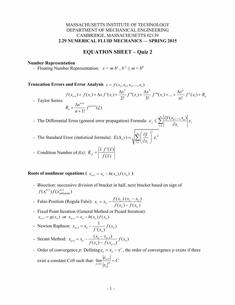
EQUATION SHEET – Quiz 2

Number Representation

- Floating Number Representation: x = m be , b-1 ≤ m < b0 Truncation Errors and Error Analysis 1 2 3( , , ,..., )ny f x x x x

- Taylor Series:

2 3

1

1( 1)

( ) ( ) '( ) ''( ) '''( ) ... ( )2! 3! !

( )1!

nn

i i i i i i n

nn

n

x x xf x f x x f x f x f x f x Rn

xR fn

- The Differential Error (general error propagation) Formula: 1

1

( ,..., )nn

y ii i

f x xx

- The Standard Error (statistical formula): 2

2

1

( )n

s ii i

fE yx

- Condition Number of f(x): '( )

( )px f xK

f x

Roots of nonlinear equations ( 1 ( ) ( )n n n nx x h x f x )

- Bisection: successive division of bracket in half, next bracket based on sign of 1 1

1 mid-point( ) ( )n nf x f x

- False-Position (Regula Falsi): ( ) ( )( ) ( )

U L Ur U

L U

f x x xx xf x f x

- Fixed Point Iteration (General Method or Picard Iteration): 1 1( ) or ( ) ( )n n n n n nx g x x x h x f x

- Newton Raphson: 11 ( )'( )n n n

n

x x f xf x

- Secant Method: 11

1

( ) ( )( ) ( )

n nn n n

n n

x xx x f xf x f x

- Order of convergence p: Defining en ne x x , the order of convergence p exists if there

exist a constant C≠0 such that: 1lim npn

n

eC

e

- 2 -

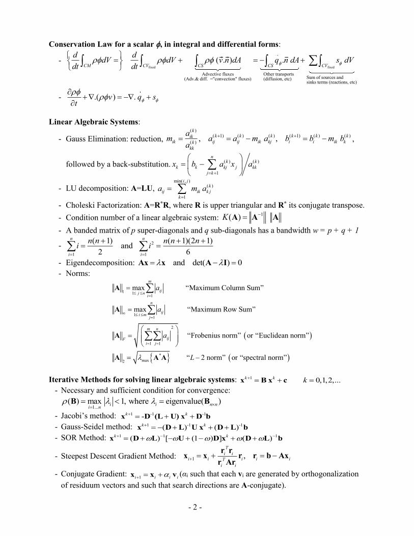
Conservation Law for a scalar , in integral and differential forms:

- fixed fixed

Advective fluxes Other transports Sum of sources and(Adv.& diff. ="convection" fluxes) (diffusion, etc)sinks terms

( . ) .CM CV CS CS CV

d ddV dV v n dA q n dA s dVdt dt

(reactions, etc)

- .( ) .v q st

Linear Algebraic Systems:

- Gauss Elimination: reduction, ( )

( 1) ( ) ( ) ( 1) ( ) ( )( ) , ,k

k k k k k kikik ij ij ik kj i i ik kk

kk

am a a m a b b m ba

,

followed by a back-substitution. ( ) ( )

1

nk k

k k kj j kkj k

x b a x a

- LU decomposition: A=LU, min( , )

( )

1

i jk

ij ik k jk

a m a

- Choleski Factorization: A=R*R, where R is upper triangular and R* its conjugate transpose. - Condition number of a linear algebraic system: 1( )K A A A - A banded matrix of p super-diagonals and q sub-diagonals has a bandwidth w = p + q + 1

- 2

1 1

( 1) ( 1)(2 1)and 2 6

n n

i i

n n n n ni i

- Eigendecomposition: and det( ) 0 Ax x A I - Norms:

1 1 1

1 1

2

1 1

*max2

max “Maximum Column Sum”

max “Maximum Row Sum”

“Frobenius norm” or “Euclidean norm”

“ 2 norm” or “spectral norm”

m

ijj n in

iji m j

m n

ijFi j

a

a

a

L

A

A

A

A A A

Iterative Methods for solving linear algebraic systems: 1 0,1,2,...k k k x B x c

- Necessary and sufficient condition for convergence:

1...( ) max 1, where eigenvalue( )i i n ni n

B B

- Jacobi’s method: 1 -1 -1-k k x D (L U) x D b - Gauss-Seidel method: 1 -1 -1( ) ( )k k x D L U x D L b - SOR Method: 1 1 1( ) [ (1 ) ] ( )k k x D L U D x D L b

- Steepest Descent Gradient Method: 1 ,T

i ii i i i iT

i i

r rx x r r b Axr Ar

- Conjugate Gradient: 1i i i i x x v (αi such that each vi are generated by orthogonalization of residuum vectors and such that search directions are A-conjugate).

- 3 -

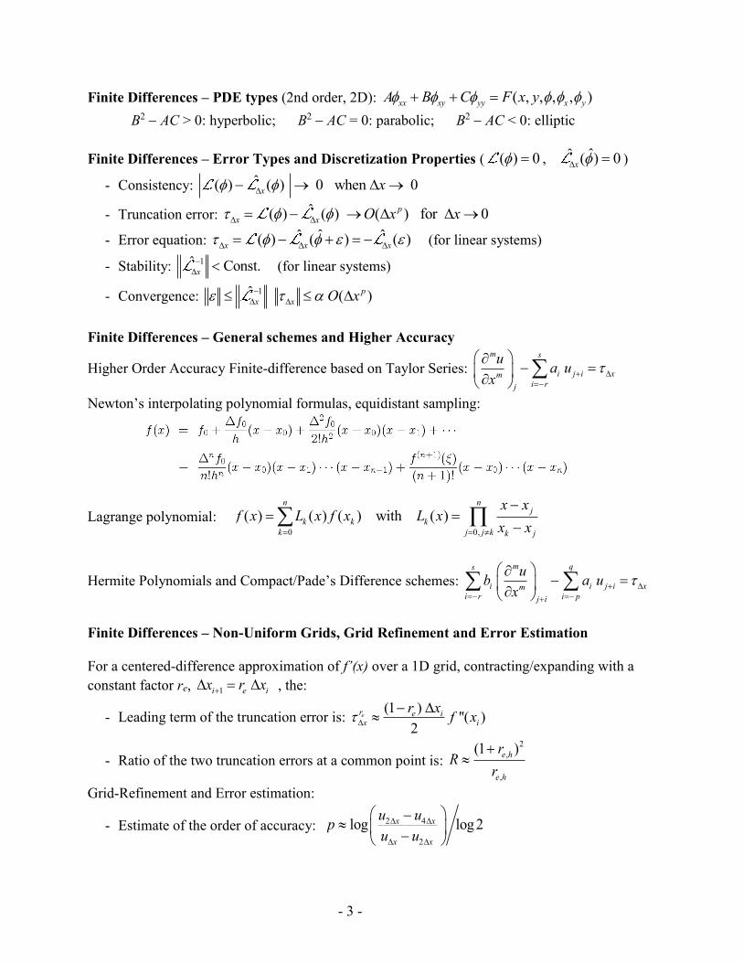
Finite Differences – PDE types (2nd order, 2D): ( , , , , )xx xy yy x yA B C F x y

B2 AC > 0: hyperbolic; B2 AC = 0: parabolic; B2 AC < 0: elliptic Finite Differences – Error Types and Discretization Properties ( ˆˆ( ) 0 , ( ) 0x )

- Consistency: ˆ( ) ( ) 0 when 0x x

- Truncation error: ˆ( ) ( ) ( ) for 0px x O x x

- Error equation: ˆˆ ˆ( ) ( ) ( )x x x (for linear systems)

- Stability: 1ˆ Const.x

(for linear systems)

- Convergence: 1ˆ ( )px x O x

Finite Differences – General schemes and Higher Accuracy

Higher Order Accuracy Finite-difference based on Taylor Series: m s

i j i xmi rj

u a ux

Newton’s interpolating polynomial formulas, equidistant sampling:

Lagrange polynomial: 0 0,

( ) ( ) ( ) with ( )n n

jk k k

k j j k k j

x xf x L x f x L x

x x

Hermite Polynomials and Compact/Pade’s Difference schemes: m qs

i i j i xmi r i pj i

ub a ux

Finite Differences – Non-Uniform Grids, Grid Refinement and Error Estimation For a centered-difference approximation of f’(x) over a 1D grid, contracting/expanding with a constant factor re, 1i e ix r x , the:

- Leading term of the truncation error is: (1 ) ''( )2

er e ix i

r x f x

- Ratio of the two truncation errors at a common point is: 2

,

,

(1 )e h

e h

rR

r

Grid-Refinement and Error estimation:

- Estimate of the order of accuracy: 2 4

2

log log2x x

x x

u upu u

- 4 -

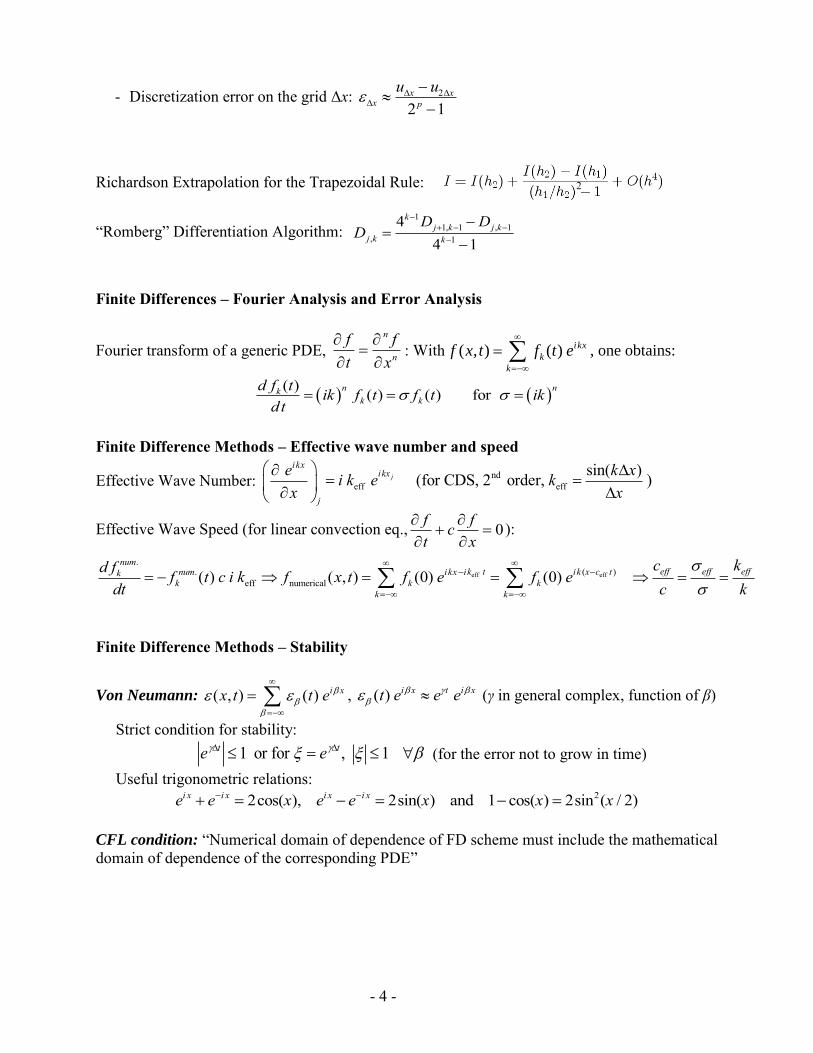
- Discretization error on the grid Δx: 2

2 1x x

x pu u

Richardson Extrapolation for the Trapezoidal Rule:

“Romberg” Differentiation Algorithm: 1

1, 1 , 1, 1

44 1

kj k j k

j k k

D DD

Finite Differences – Fourier Analysis and Error Analysis

Fourier transform of a generic PDE, n

nf ft x

: With

( ) ( ) ( ) for n nk

k kd f t ik f t f t ik

d t

Finite Difference Methods – Effective wave number and speed

Effective Wave Number: ndeff eff

sin( ) (for CDS, 2 order, )jikx

ikx

j

e k xi k e kx x

Effective Wave Speed (for linear convection eq., 0f fct x

):

eff eff

.(. )

eff numerical( ) ( , ) (0) (0)num

eff eff effk t ik x cnum ikx i tkk k k

k k

c kd f f t c i k f x t f e f edt c k

Finite Difference Methods – Stability

Von Neumann: ( , ) ( ) i xx t t e

, ( ) i x t i xt e e e

(γ in general complex, function of β)

Strict condition for stability: 1 or for , 1t te e (for the error not to grow in time)

Useful trigonometric relations: 22cos( ), 2sin( ) and 1 cos( ) 2sin ( / 2)i x i x i x i xe e x e e x x x

CFL condition: “Numerical domain of dependence of FD scheme must include the mathematical domain of dependence of the corresponding PDE”

2

f (x, t) f ( ) i kx

k t ek

, one obtains:

PFJL Lecture 10, 15Numerical Fluid Mechanics2.29

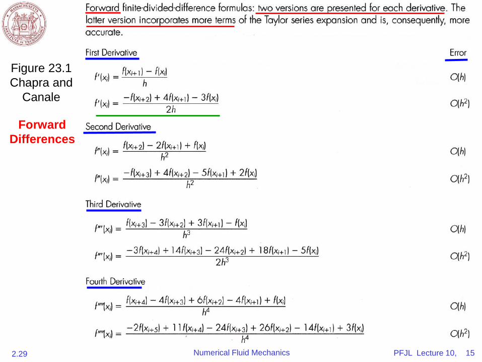
Figure 23.1

Chapra and

Canale

Forward

Differences

PFJL Lecture 10, 16Numerical Fluid Mechanics2.29

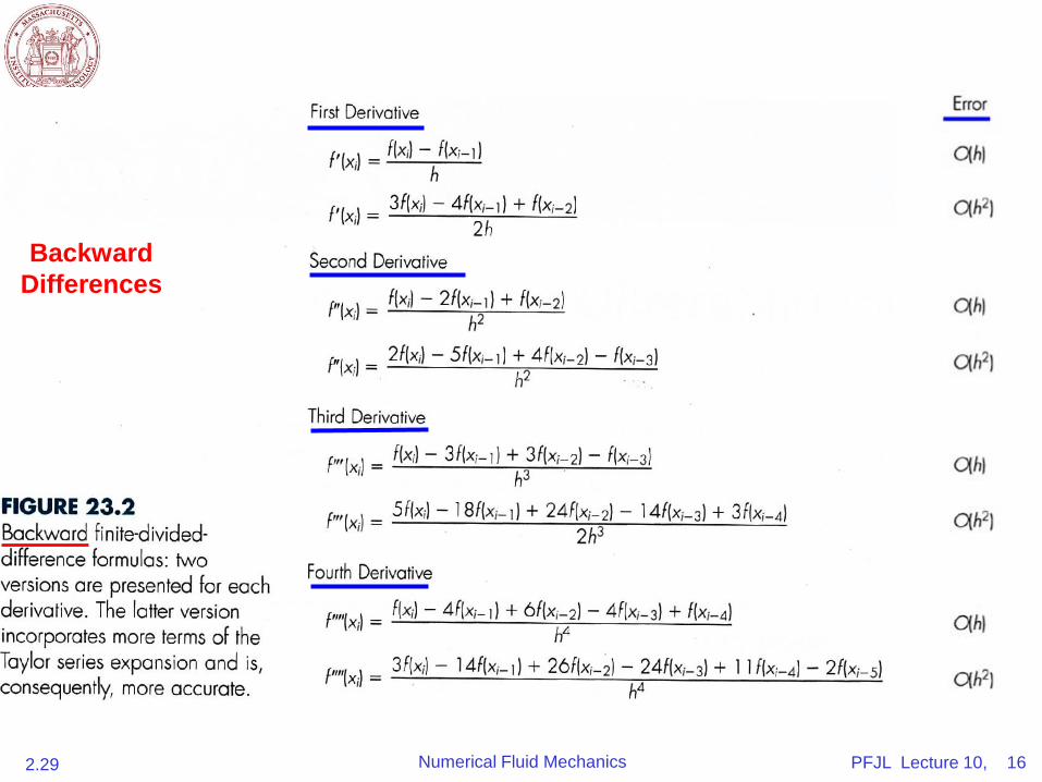
Backward

Differences

PFJL Lecture 10, 17Numerical Fluid Mechanics2.29

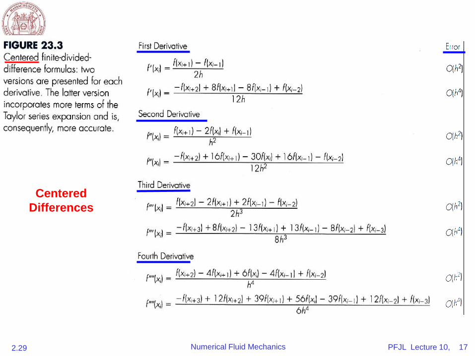
Centered

Differences

- 8 -

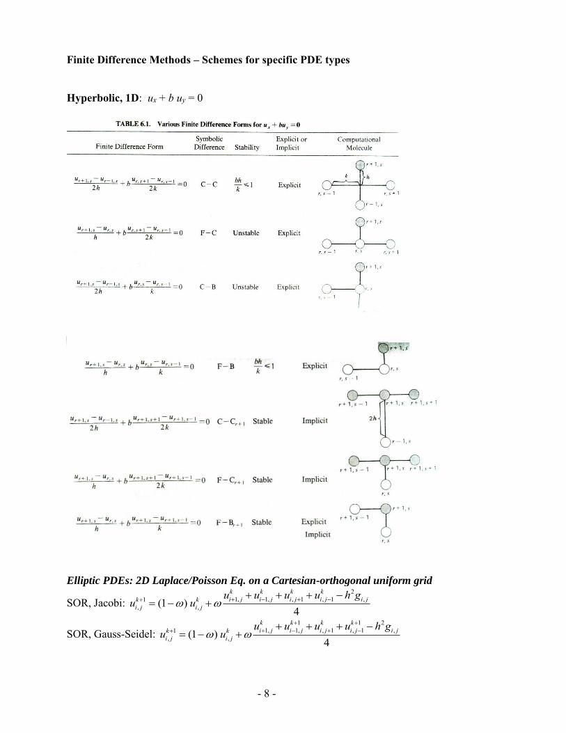
Finite Difference Methods – Schemes for specific PDE types Hyperbolic, 1D: ux + b uy = 0

Elliptic PDEs: 2D Laplace/Poisson Eq. on a Cartesian-orthogonal uniform grid

SOR, Jacobi: 2

1, 1, , 1 , 1 ,1, ,(1 )

4

k k k ki j i j i j i j i jk k

i j i j

u u u u h gu u

SOR, Gauss-Seidel: 1 1 2

1, 1, , 1 , 1 ,1, ,(1 )

4

k k k ki j i j i j i j i jk k

i j i j

u u u u h gu u

- 9 -

Parabolic PDEs: 2D Heat Conduction Eq. on a Cartesian-orthogonal grid

• Explicit:1

, , 1, , 1, , 1 , , 12 22 2

2 2n n n n n n n ni j i j i j i j i j i j i j i jT T T T T T T T

c ct x y

• Crank-Nicolson Implicit (for Δx=Δy, with2

2t crx

):

1 1 1 1 1, , 1, 1, , 1 , 1 1, 1, , 1 , 1(1 2 ) (1 2 )

2 2n n n n n n n n n n

i j i j i j i j i j i j i j i j i j i jr rr T r T T T T T T T T T

• ADI: 1/ 2 1/ 2 1/ 2 1/ 2

, , 1, , 1, , 1 , , 12 22 2

2 2/ 2

n n n n n n n ni j i j i j i j i j i j i j i jT T T T T T T T

c ct x y

1 1/ 2 1 1 1 1/ 2 1/ 2 1/ 2, , 1, , 1, , 1 , , 12 2

2 2

2 2/ 2

n n n n n n n ni j i j i j i j i j i j i j i jT T T T T T T T

c ct x y

(for Δx=Δy): 1/2 1/2 1/2, 1 , , 1 1, , 1,2(1 ) 2(1 )n n n n n n

i j i j i j i j i j i jrT r T rT rT r T rT

1 1 1 1/2 1/2 1/2

1, , 1, , 1 , , 12(1 ) 2(1 )n n n n n ni j i j i j i j i j i jrT r T rT rT r T rT

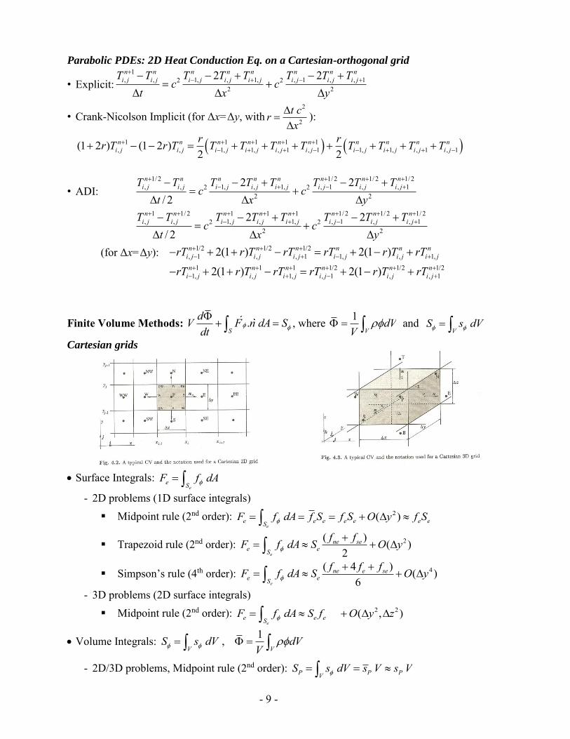
Finite Volume Methods: .S

dV F n dA Sdt

, where 1

VdV

V and

VS s dV

Cartesian grids

Surface Integrals:

ee S

F f dA

- 2D problems (1D surface integrals) Midpoint rule (2nd order): 2( )

ee e e e e e eS

F f dA f S f S O y f S

Trapezoid rule (2nd order): 2( ) ( )2e

ne see eS

f fF f dA S O y

Simpson’s rule (4th order): 4( 4 ) ( )6e

ne e see eS

f f fF f dA S O y

- 3D problems (2D surface integrals) Midpoint rule (2nd order): 2 2( , )

ee e eS

F f dA S f O y z

Volume Integrals: 1,V V

S s dV dVV

- 2D/3D problems, Midpoint rule (2nd order): P P PVS s dV s V s V

- 10 -

- 2D, bi-quadratic (4th order, Cart.): 16 4 4 4 436P P s n w e se sw ne nwx yS s s s s s s s s s

Interpolations / Differentiations (obtain fluxes “Fe= f (e)” as a function of cell-average values)

- Upwind Interpolation (UDS):

if . 0

if . 0P e

eE e

v n

v n

- Linear Interpolation (CDS): (1 ) where e Pe E e P e e

E P

x xx x

(1 ), with PE P

E P

x xx x

E P

e E Px x x

- Quadratic Upwind interpolation (QUICK): 1 2( ) ( )e U D U U UUg g

For uniform grids, 3 3

33

6 3 1 38 8 8 48e U D UU

D

x Rx

- Higher order schemes: For example, for 2 3

0 1 2 3( )x a a x a x a x ,

Convective fluxes 27 27 3 348

P E W EEe

Diffusive Fluxes, for a uniform Cartesian grid: 27 2724

E P W EE

ex x

.

For a compact high order scheme: 4( )2 8

P Ee

P E

x O xx x

Solution of the Navier-Stokes Equations

Newtonian fluid + incompressible + constant: 2.( )

. 0

v v v p v gtv

Strong conservative form, general Newtonian fluid: 2.( ) .3

j ji ii i j i i i i

j i j

u uv uv v p e e e g x et x x x

Kinetic energy equation, CV form:

2 2

( . ) . ( . ). : . .2 2CV CS CS CS CV

v vdV v n dA p v n dA v n dA v p v g v dV

t

Pressure equation: 2 2. . . .( ) . .vp p v v v gt

For constant μ and ρ: . . .( )p v v

- 11 -

Pressure-correction Methods

( )+ i j ij

ij j

u uH

x x

Forward-Euler Explicit in Time:

1n

n n ni i i

i

n ni

i i i

pu u t Hx

p Hx x x

Backward-Euler Implicit in Time:

1 1 1

1

1 11

( )+

( )

n n nn n i j ij

i ij j i

n nni j ij

i i i j j

u u pu u tx x x

u upx x x x x

Backward-Euler Implicit in Time, linearized momentum update:

1 ( ) ( ) ( )n nn n n

n n i j i j i j ij iji i i

j j j j j i i

u u u u u u p pu u u tx x x x x x x

Steady state solver, matrix notation:

Outer iteration, nonlinear solve: *

*

1* 1m

imi

mm mi

i

px

u

u

δA u bδ

Outer iteration, pressure update: * *

*

* 1 1* 1,

m mi i

mi

mmm mii

i i i

px x x

u uu

δ u δ δA u A bδ δ δ

Inner iteration, linear solve: *

*

mi

mi

mm mi

i

px

u

u

δA u bδ

Steady state solver, matrix notation, pressure-correction schemes:

Based on the above, but introduce um m *

i iu u '

get varied schemes (SIMPLE, SIMPLER, SIMPLEC, PISO, etc.)

pm mp 1 p ' and further simplify to

- 12 -

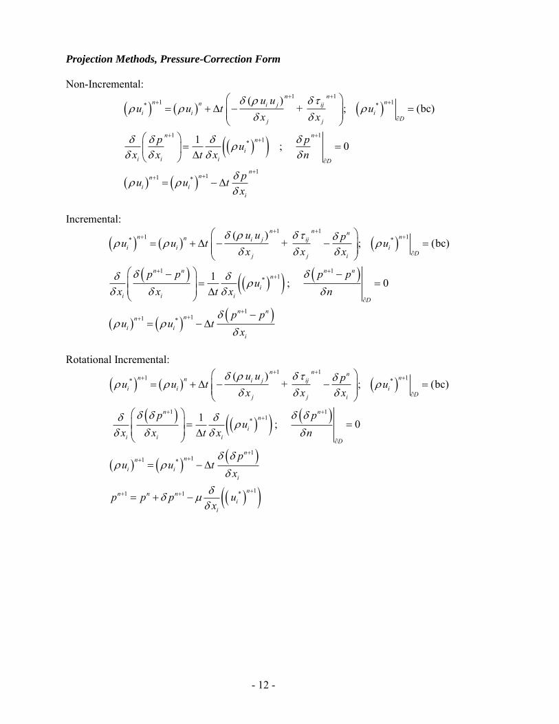
Projection Methods, Pressure-Correction Form

Non-Incremental:

1 11 1* *

1 11*

111 *

( )+ ; (bc)

1 ; 0

n nn nn i j ij

i i iDj j

n nn

ii i i D

nnn

i ii

u uu u t u

x x

p pux x t x n

pu u tx

Incremental:

1 11 1* *

1 11*

111 *

( )+ ; (bc)

1 ; 0

n n nn nn i j iji i i

Dj j i

n n n nn

ii i i D

n nnn

i ii

u u pu u t ux x x

p p p pu

x x t x n

p pu u t

x

Rotational Incremental:

1 11 1* *

1 11*

111 *

11 1 *

( )+ ; (bc)

1 ; 0

n n nn nn i j iji i i

Dj j i

n nn

ii i i D

nnn

i ii

nn n ni

i

u u pu u t ux x x

p pu

x x t x n

pu u t

x

p p p ux

MIT OpenCourseWarehttp://ocw.mit.edu

2.29 Numerical Fluid MechanicsSpring 2015

For information about citing these materials or our Terms of Use, visit: http://ocw.mit.edu/terms.