ePubWU Institutional Repository

Christoph Bremberger and Francisca Bremberger and Mikulas Luptacik andStephan Schmitt

Regulatory impact of environmental standards on the eco-efficiency of firms

Article (Accepted for Publication)(Refereed)

Original Citation:Bremberger, Christoph and Bremberger, Francisca and Luptacik, Mikulas and Schmitt, Stephan(2014) Regulatory impact of environmental standards on the eco-efficiency of firms. Journal of theOperational Research Society, 66 (3). pp. 421-433. ISSN 0160-5682

This version is available at: http://epub.wu.ac.at/4536/Available in ePubWU: May 2015

ePubWU, the institutional repository of the WU Vienna University of Economics and Business, isprovided by the University Library and the IT-Services. The aim is to enable open access to thescholarly output of the WU.

This document is the version accepted for publication and — in case of peer review — incorporatesreferee comments. There are minor differences between this and the publisher version which couldhowever affect a citation.

http://epub.wu.ac.at/

Regulatory impact of environmental standards on

the eco-efficiency of firms

Keywords: Data envelopment analysis, Environmental studies, Energy, Regulation

Abstract

In this paper we propose an approach to implement environmental standards into Data Envelopment

Analysis (DEA) and in this way to measure their regulatory impact on eco-efficiency of firms. As one

standard feature of basic DEA models (as e.g. CCR from Charnes et al. (1978)) lies in the exogeneity

of inputs, desirable and undesirable outputs, it is not possible to introduce environmental constraints

for these parameters directly into basic DEA models. Therefore, we use a bounded-variable way, which

allows constraints on the efficiency frontier. The regulatory impact is assessed as difference in eco-

efficiency scores before and after fictive introduction of an environmental standard. Furthermore, we

distinguish between weak and strong disposability of undesirable outputs and develop corresponding

models.

Assessing the regulatory impact of environmental standards in advance provides support for en-

vironmental policy makers in choosing appropriate instruments and in adjusting the intensity of

regulation.1

1The authors are thankful for helpful comments of the participants of the EWEPA 2011 Conference in Verona and theInternational Conference on Operations Research 2011 in Zurich.

1

1 Introduction

In today’s political debates the concept of sustainability has become indispensable. The basic idea be-

hind this concept is that natural resources are finite and that ecological issues – in particular pollution

– cannot be ignored any more. In many cases the destruction of ecological capital leads contempora-

neously to an increase in gross domestic product and if there are no costs associated with the former,

long-term environmental costs are completely excluded from economic analysis. Therefore, one of the

most striking challenges in (environmental) economics is the internalisation of negative external effects.

Various concepts and models try to deal with this issue. Our paper enters into the discussion as we

refer to implementing environmental standards in evaluating the eco-efficiency2 of different firms in a

particular industry in order to give incentives for less pollutant production. Moreover, in this way it is

possible to measure the regulatory impact on firms by comparing eco-efficiency scores before and after

a fictive introduction of an environmental standard. This can provide support for the environmental

policy makers in choosing appropriate instruments and intensity of regulation. As it is rather difficult

to quantify pollution, emissions or other undesirable outputs in monetary units, we refer to Data En-

velopment Analysis (DEA), a non-parametric approach for multilateral productivity comparisons. With

this approach, which is extended in several ways, it is now possible to ascertain the eco-efficiency of firms.

The remainder of the article is organised as follows. The next Section provides a brief literature overview

in DEA with a special focus on the measurement of eco-efficiency and the effects of regulatory standards.

Section 3 presents our basic idea using a fictive example of eight DMUs, wherein several variants of DEA-

models that deal with undesirable outputs in the context of eco-efficiency are applied and discussed.

In Section 4 we show how to implement our idea by extending common slack-based measure models in

the DEA field. Finally, the most important findings are summarised and drawn together in a principal

conclusion.

2 Literature

At the beginning the main purpose of the non-parametric Data Envelopment Analysis (DEA), which

is a linear programming technique going back to Charnes et al. (1978) and which is highly applied in

benchmarking analysis, has been on estimating efficiency and productivity. Meanwhile, it also has been

widely used for environmental analysis and the estimation of eco-efficiency, where – apart from inputs

and desirable (good) outputs – undesirable (bad) outputs such as pollution or emissions come into play.

One can distinguish various approaches in the literature that deal with this issue, see e.g. Tyteca (1996)

and Sahoo et al. (2011).3 Central to all these considerations is the differentiation between strong and

weak disposability of outputs (Fare et al. (1986), Fare et al. (1989), Fare and Grosskopf (2003), Fare and

Grosskopf (2004), Fare and Grosskopf (2009)). Strong disposability assumes that the reduction in bad

outputs is not associated with any direct costs. In contrast, the basic idea behind weak disposability is

that, given a certain amount of inputs, the higher the ratio between desirable and undesirable output the

higher is efficiency. In other words, firms should be penalised for the production of bad outputs, whereas

higher production of (good) outputs, as usually, should have a positive effect on efficiency.

Depending on the kind of disposability one can further distinguish different approaches how to include bad

2Korhonen and Luptacik (2004) define eco-efficiency according to Heinz Felsner: We are looking for eco-efficient solutionssuch that the goods and services can be produced with less energy and resources and with less waste and emission.

3For a survey of DEA studies in the area of energy and environment, see Zhou et al. (2008).

2

outputs into the DEA framework, see e.g. Scheel (2001) and Sahoo et al. (2011). According to Korhonen

and Luptacik (2004) undesirable outputs can either be treated as negative outputs (Koopmans (1951)) or

as inputs (Cropper and Oates (1992)). While the explanation for the former is more intuitive at the first

glance (all else equal, a higher amount of negative outputs has a negative impact on overall efficiency),

undesirable outputs can also be interpreted as inputs since both incur costs. Within this logic one tries to

produce a given level of output with minimal inputs and undesirable outputs. Analyzing 24 power plants

in a European country, the main result of Korhonen and Luptacik (2004) was that the efficiency frontier,

unlike the individual efficiency scores, is independent of the way of including undesirable outputs, at least

for the specifications they consider. Moreover, bad outputs can also be taken into account in form of

their reciprocals (Golany and Roll (1989)) or the negative outputs can be subtracted from a sufficient

large number (Ali and Seliford (1990)). However, Dyson et al. (2001) show for a simple example that

these additional ways of incorporating bad outputs can result in different efficiency frontiers, with varying

numbers of efficient units. In summary, all these approaches and specifications of bad output modelling

have their individual pros and cons, see e.g. Dyson et al. (2001), Hailu and Veeman (2001), Hailu (2003),

Fare and Grosskopf (2003), and Forsund (2008), indicating that there is no first-best approach for every

situation and under all circumstances.

A number of recent studies introduce further developments of the basic ideas of Fare et al. (1989). Lozano

and Gutierrez (2011) developed a modified slack–based DEA model, which assumes joint weak disposabil-

ity of the desirable and undesirable outputs to compare the efficiencies of airports. Kuosmanen (2005)

introduced a DEA model extension that allows for non-uniform abatement factors of weak disposable

bad outputs. Thereby, not all firms have to make use of the same abatement factors, instead different

technologies and circumstances can be taken into account. Similarly, Yang and Pollitt (2010) point out

that it is important to account for technically correct disposability features of the undesirable outputs.

Analysing a set of Chinese coal–fired power plants, they showed that efficiency scores changed signifi-

cantly once uniform disposability of all undesirable outputs has been assumed.

Benchmarking and environmental analysis using DEA is not only restricted to the modeling of undesirable

outputs. Moreover, it is possible to incorporate regulatory standards into the DEA framework, which

ensure that a certain level of emissions is not exceeded or that certain regulatory requirements are

fulfilled. With regard to the latter, Fare and Logan (1992) introduced a maximum allowed rate-of-return

as regulatory constraint into the DEA setting. Hereby, the underlying cost frontier is cut in such a

way that all firms that are located on the new frontier have to meet the regulatory constraint, which is

externally set by the regulator. The regulatory impact of the constraint on technical efficiency is estimated

by dividing the unregulated technical efficiency score through the regulated one.4 The approach of Fare

and Logan (1992) is based on a former paper of the two authors, Fare and Logan (1983), who defined

a rate-of-return regulated production function and proved its existence. Ouellette and Vigeant (2001)

extended the regulated production function to a general set of regulatory constraints. A summary of

their ideas can be found in Ouellette et al. (2009), who present regulated input (B(y, k, r)) and output

(D(x, k, r)) sets as intersection between sets describing what ”the technology and the regulation allow”:

4The same procedure can also be applied to derive the regulatory impact on allocative and overall efficiency respectively.

3

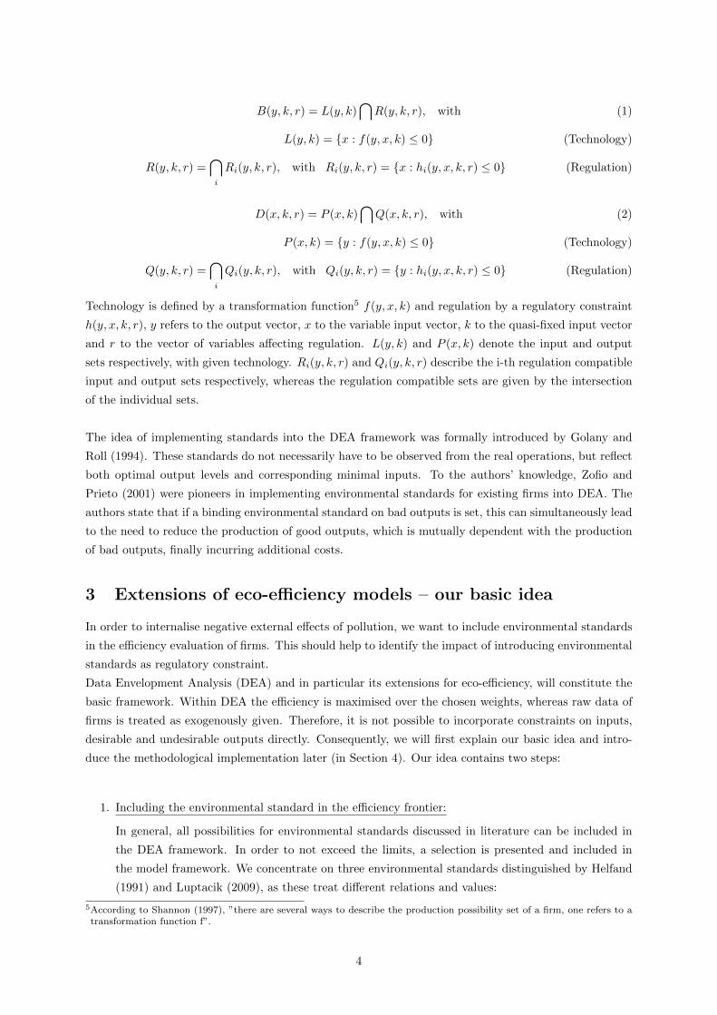
B(y, k, r) = L(y, k)⋂R(y, k, r), with (1)

L(y, k) = {x : f(y, x, k) ≤ 0} (Technology)

R(y, k, r) =⋂i

Ri(y, k, r), with Ri(y, k, r) = {x : hi(y, x, k, r) ≤ 0} (Regulation)

D(x, k, r) = P (x, k)⋂Q(x, k, r), with (2)

P (x, k) = {y : f(y, x, k) ≤ 0} (Technology)

Q(y, k, r) =⋂i

Qi(y, k, r), with Qi(y, k, r) = {y : hi(y, x, k, r) ≤ 0} (Regulation)

Technology is defined by a transformation function5 f(y, x, k) and regulation by a regulatory constraint

h(y, x, k, r), y refers to the output vector, x to the variable input vector, k to the quasi-fixed input vector

and r to the vector of variables affecting regulation. L(y, k) and P (x, k) denote the input and output

sets respectively, with given technology. Ri(y, k, r) and Qi(y, k, r) describe the i-th regulation compatible

input and output sets respectively, whereas the regulation compatible sets are given by the intersection

of the individual sets.

The idea of implementing standards into the DEA framework was formally introduced by Golany and

Roll (1994). These standards do not necessarily have to be observed from the real operations, but reflect

both optimal output levels and corresponding minimal inputs. To the authors’ knowledge, Zofio and

Prieto (2001) were pioneers in implementing environmental standards for existing firms into DEA. The

authors state that if a binding environmental standard on bad outputs is set, this can simultaneously lead

to the need to reduce the production of good outputs, which is mutually dependent with the production

of bad outputs, finally incurring additional costs.

3 Extensions of eco-efficiency models – our basic idea

In order to internalise negative external effects of pollution, we want to include environmental standards

in the efficiency evaluation of firms. This should help to identify the impact of introducing environmental

standards as regulatory constraint.

Data Envelopment Analysis (DEA) and in particular its extensions for eco-efficiency, will constitute the

basic framework. Within DEA the efficiency is maximised over the chosen weights, whereas raw data of

firms is treated as exogenously given. Therefore, it is not possible to incorporate constraints on inputs,

desirable and undesirable outputs directly. Consequently, we will first explain our basic idea and intro-

duce the methodological implementation later (in Section 4). Our idea contains two steps:

1. Including the environmental standard in the efficiency frontier:

In general, all possibilities for environmental standards discussed in literature can be included in

the DEA framework. In order to not exceed the limits, a selection is presented and included in

the model framework. We concentrate on three environmental standards distinguished by Helfand

(1991) and Luptacik (2009), as these treat different relations and values:

5According to Shannon (1997), ”there are several ways to describe the production possibility set of a firm, one refers to atransformation function f”.

4

• Intensity regulation: EmissionInput ≤ α1

• Emission per unit of output: EmissionOutput ≤ α2

• Set level of emissions:6 Emission ≤ α3

Under intensity regulation introduced by Dudenhoffer (1984), the emissions per unit of input have

to be set below a predefined benchmark. Therefore, firms which have already invested in less

polluting technologies in the past have an advantage. Under the second alternative, emissions per

unit of output should not be higher than a given value. In this case, it is not clear that the level of

emission will fall, since emissions can increase as long as output rises. Third, the absolute amount

of emissions can be reduced with the consequence that all emission producing firms are treated

equally independently of what they have done in the past in order to cut emissions.

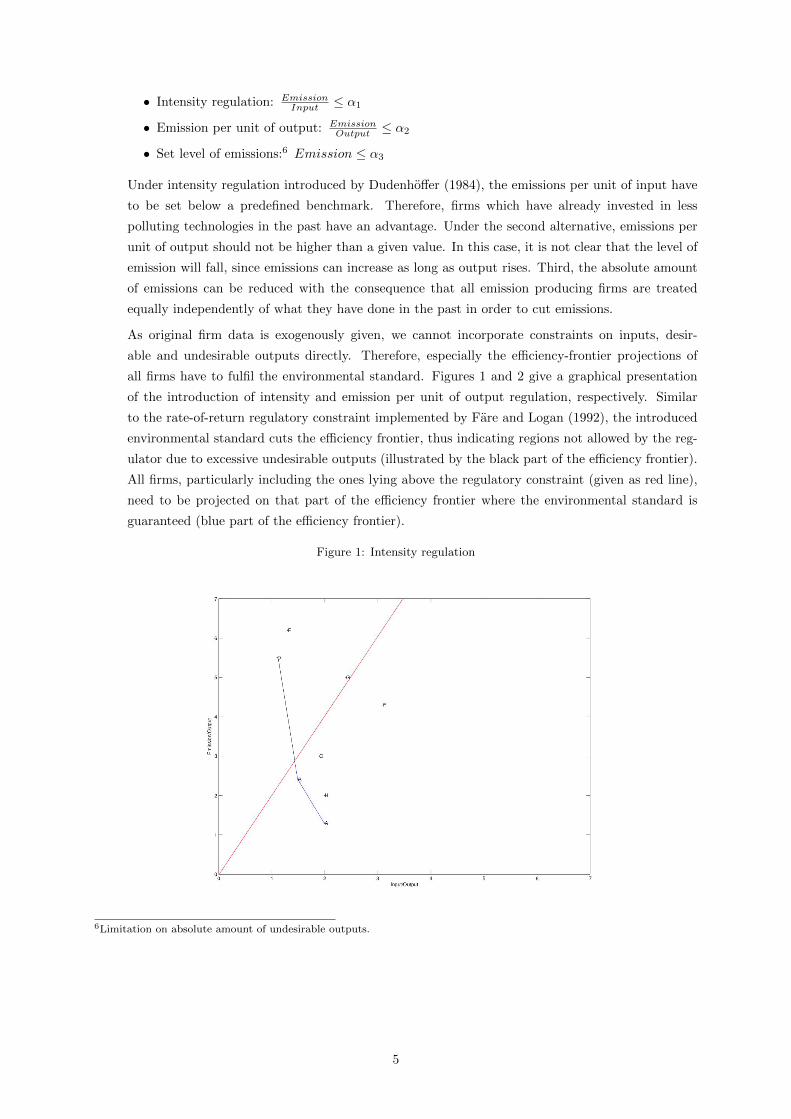
As original firm data is exogenously given, we cannot incorporate constraints on inputs, desir-

able and undesirable outputs directly. Therefore, especially the efficiency-frontier projections of

all firms have to fulfil the environmental standard. Figures 1 and 2 give a graphical presentation

of the introduction of intensity and emission per unit of output regulation, respectively. Similar

to the rate-of-return regulatory constraint implemented by Fare and Logan (1992), the introduced

environmental standard cuts the efficiency frontier, thus indicating regions not allowed by the reg-

ulator due to excessive undesirable outputs (illustrated by the black part of the efficiency frontier).

All firms, particularly including the ones lying above the regulatory constraint (given as red line),

need to be projected on that part of the efficiency frontier where the environmental standard is

guaranteed (blue part of the efficiency frontier).

Figure 1: Intensity regulation

6Limitation on absolute amount of undesirable outputs.

5

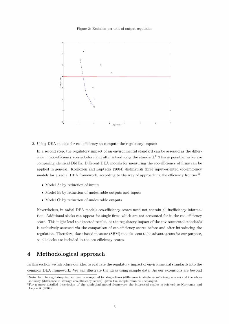
Figure 2: Emission per unit of output regulation

2. Using DEA models for eco-efficiency to compute the regulatory impact:

In a second step, the regulatory impact of an environmental standard can be assessed as the differ-

ence in eco-efficiency scores before and after introducing the standard.7 This is possible, as we are

comparing identical DMUs. Different DEA models for measuring the eco-efficiency of firms can be

applied in general. Korhonen and Luptacik (2004) distinguish three input-oriented eco-efficiency

models for a radial DEA framework, according to the way of approaching the efficiency frontier:8

• Model A: by reduction of inputs

• Model B: by reduction of undesirable outputs and inputs

• Model C: by reduction of undesirable outputs

Nevertheless, in radial DEA models eco-efficiency scores need not contain all inefficiency informa-

tion. Additional slacks can appear for single firms which are not accounted for in the eco-efficiency

score. This might lead to distorted results, as the regulatory impact of the environmental standards

is exclusively assessed via the comparison of eco-efficiency scores before and after introducing the

regulation. Therefore, slack-based measure (SBM) models seem to be advantageous for our purpose,

as all slacks are included in the eco-efficiency scores.

4 Methodological approach

In this section we introduce our idea to evaluate the regulatory impact of environmental standards into the

common DEA framework. We will illustrate the ideas using sample data. As our extensions are beyond

7Note that the regulatory impact can be computed for single firms (difference in single eco-efficiency scores) and the wholeindustry (difference in average eco-efficiency scores), given the sample remains unchanged.

8For a more detailed description of the analytical model framework the interested reader is referred to Korhonen andLuptacik (2004).

6

common solver software packages, we generated all results by solving the models in GAMS (General

Algebraic Modeling System).

As argued before, SBM models are more advantageous than radial models for our purpose, because all

slacks are accounted for in the eco-efficiency score. Therefore, we use the Undesirable Output Model from

Cooper et al. (2007) and a slack-based measure version of Model B from Korhonen and Luptacik (2004)

as starting points. The underlying technology refers to constant returns to scale (CRS technology), but

all presented models can be adjusted to variable returns to scale (VRS technology) if this appears more

realistic for a certain indstry. For all presented models the following definitions hold:

• m total number of inputs, s1 total number of good outputs, s2 total number of bad outputs

• x input, yg good oupt, yb bad output

• i input index xi (i = 1, 2, ...,m), r index for good oupts ygr (k = 1, 2, ..., s1) and bad outputs

ybr (r = 1, 2, ..., s2)

• the subscript ”o”’ indicates the distinct firm currently under observation (e.g. xo)

• s− input slack, sg good output slack, sb bad output slack, sWD weak disposability slack

• λ weights on firms, λj weight on firm j (j = 1, 2, ..., n)

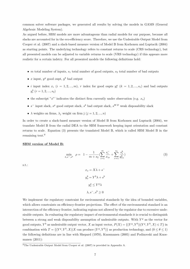
In order to create a slack-based measure version of Model B from Korhonen and Luptacik (2004), we

translate Model B from the radial DEA to the SBM framework keeping input orientation and constant

returns to scale. Equation (3) presents the translated Model B, which is called SBM Model B in the

remaining text.9

SBM version of Model B:

minλ,s−,sb

ρ = 1− 1

m+ s2(

m∑i=1

s−ixio

+

s2∑r=1

sbrybro

) (3)

s.t.:

xo = Xλ+ s−

ybo = Y bλ+ sb

ygo ≤ Y gλ

λ, s−, sb ≥ 0

We implement the regulatory constraint for environmental standards by the idea of bounded variables,

which allows constraints on efficiency-frontier projections. The effect of the environmental standard is an

intersection of the efficiency frontier, indicating regions not allowed by the regulator due to excessive unde-

sirable outputs. In evaluating the regulatory impact of environmental standards it is crucial to distinguish

between a strong and weak disposability assumption of undesirable outputs. With Y g as the vector for

good outputs, Y b as undesirable output vector, X as input vector, P (X) = {(Y g, Y b)|(Y g, Y b, X) ∈ T} in

combination with T = {(Y g, Y b, X)|X can produce (Y g, Y b)} as production technology, and (0 ≤ θ ≤ 1)

the following definitions are in line with Shepard (1970), Kuosmanen (2005) and Podinovski and Kuos-

manen (2011):

9The Undesirable Output Model from Cooper et al. (2007) is provided in Appendix A.

7

Undesirable outputs are strongly disposable if:

(Y g, Y b) ∈ P (X) implies (Y g, θY b) ∈ P (X), which means

(Y g, Y b, X) ∈ T implies (Y g, θY b, X) ∈ T .

Undesirable outputs are weakly disposable via outputs if:

(Y g, Y b) ∈ P (X) implies (θY g, θY b) ∈ P (X), which means

(Y g, Y b, X) ∈ T implies (θY g, θY b, X) ∈ T .

Undesirable outputs are weakly disposable via inputs if:10

(Y g, Y b, X) ∈ T implies (Y g, θY b, 1θX) ∈ T .

This means that strongly disposable undesirable outputs can be reduced at no cost, whereas weakly dis-

posable undesirable outputs can only be decreased when simultaneously decreasing outputs or increasing

inputs.

4.1 Strong disposability assumption

If strong disposability of undesirable outputs is assumed, the regulatory impact of environmental stan-

dards can be assessed as the difference of eco-efficiency scores between standard SBM models (SBM

Model B from Equation (3) and the Undesirable Output Model from Cooper et al. (2007)), and modified

versions including the environmental standard. Herein, all environmental standards (intensity, emission

per unit of output and level-of-emission regulation) can be implemented in a bounded-variable way.

4.1.1 SBM Model B

In order to extend the SBM Model B by the environmental standard we add a fourth constraint consti-

tuting that projections on the efficiency frontier need to fulfil the environmental standard. In Equation

(4) the environmental standard is given as emission per unit of output regulation.11 This extended SBM

Model B is called SBM Model B bounded in the remaining text.

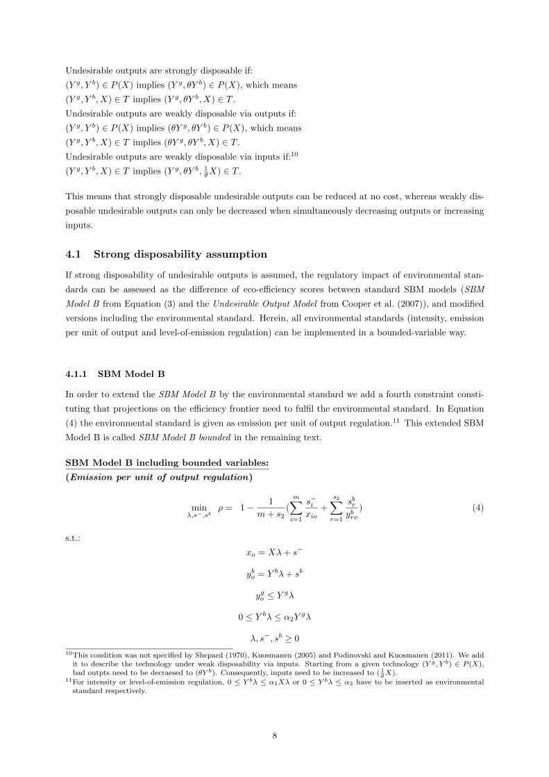
SBM Model B including bounded variables:

(Emission per unit of output regulation)

minλ,s−,sb

ρ = 1− 1

m+ s2(

m∑i=1

s−ixio

+

s2∑r=1

sbrybro

) (4)

s.t.:

xo = Xλ+ s−

ybo = Y bλ+ sb

ygo ≤ Y gλ

0 ≤ Y bλ ≤ α2Ygλ

λ, s−, sb ≥ 0

10This condition was not specified by Shepard (1970), Kuosmanen (2005) and Podinovski and Kuosmanen (2011). We addit to describe the technology under weak disposability via inputs. Starting from a given technology (Y g , Y b) ∈ P (X),bad outpts need to be decraesed to (θY b). Consequently, inputs need to be increased to ( 1

θX).

11For intensity or level-of-emission regulation, 0 ≤ Y bλ ≤ α1Xλ or 0 ≤ Y bλ ≤ α3 have to be inserted as environmentalstandard respectively.

8

Sample data In this section we will illustrate our ideas using – for simplicity and without loss of

generality – a fictive12 example of eight firms using one input to produce one desirable output and one

type of emission. To avoid a loss of generality we include all relevant (extreme) cases to demonstrate the

characteristics of our approach. Table 1 summarises the data of the DMUs used. As we will deal with

emission per unit of output as well as intensity regulation, the last two columns constitute the respective

measures.

Table 1: Data of DMUs

Input Emissions Output EmissionOutput

EmissionInput

A 20 13 10 1.3 0.7

B 15 24 10 2.4 1.6

C 19 30 10 3 1.6

D 11 55 10 5.5 5

E 13 62 10 6.2 4.8

F 31 43 10 4.3 1.4

G 24 50 10 5 2.1

H 20 20 10 2 1

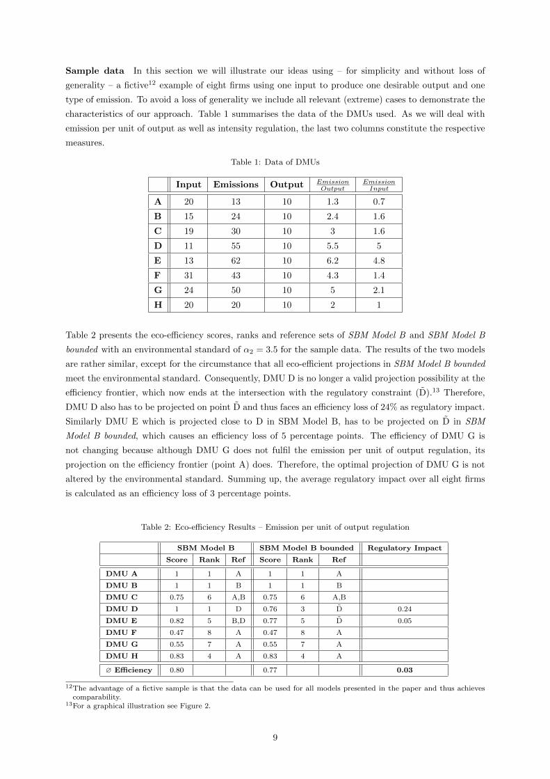
Table 2 presents the eco-efficiency scores, ranks and reference sets of SBM Model B and SBM Model B

bounded with an environmental standard of α2 = 3.5 for the sample data. The results of the two models

are rather similar, except for the circumstance that all eco-efficient projections in SBM Model B bounded

meet the environmental standard. Consequently, DMU D is no longer a valid projection possibility at the

efficiency frontier, which now ends at the intersection with the regulatory constraint (D).13 Therefore,

DMU D also has to be projected on point D and thus faces an efficiency loss of 24% as regulatory impact.

Similarly DMU E which is projected close to D in SBM Model B, has to be projected on D in SBM

Model B bounded, which causes an efficiency loss of 5 percentage points. The efficiency of DMU G is

not changing because although DMU G does not fulfil the emission per unit of output regulation, its

projection on the efficiency frontier (point A) does. Therefore, the optimal projection of DMU G is not

altered by the environmental standard. Summing up, the average regulatory impact over all eight firms

is calculated as an efficiency loss of 3 percentage points.

Table 2: Eco-efficiency Results – Emission per unit of output regulation

SBM Model B SBM Model B bounded Regulatory Impact

Score Rank Ref Score Rank Ref

DMU A 1 1 A 1 1 A

DMU B 1 1 B 1 1 B

DMU C 0.75 6 A,B 0.75 6 A,B

DMU D 1 1 D 0.76 3 D 0.24

DMU E 0.82 5 B,D 0.77 5 D 0.05

DMU F 0.47 8 A 0.47 8 A

DMU G 0.55 7 A 0.55 7 A

DMU H 0.83 4 A 0.83 4 A

∅ Efficiency 0.80 0.77 0.03

12The advantage of a fictive sample is that the data can be used for all models presented in the paper and thus achievescomparability.

13For a graphical illustration see Figure 2.

9

To evaluate the regulatory impact of the emission per unit of output regulation, it is necessary to solve

SBM Model B bounded for different values of α2. If α2 is for instance set to 1.5, the overall regulatory

impact amounts to 12 percentage points, which is around four times the effect of an environmental

standard of α2 = 3.5. For α2 = 1, which would indicate that outputs and undesirable outputs need

to be equal, it would be most efficient for all firms to cease production and leave the market. Detailed

information about efficiency scores and regulatory impacts of different environmental standards can be

found in Appendix B.

4.1.2 Undesirable Output Model

The Undesirable Output Model from Cooper et al. (2007) is extended in a similar way. Again, one

additional constraint on the set of possible projections is added. This fourth constraint determines that

projections on the efficiency frontier need to fulfil the environmental standard. In Equation (5) the

environmental standard is given as intensity regulation.14 This modified model is called Undesirable

Output Model bounded in the remaining text.

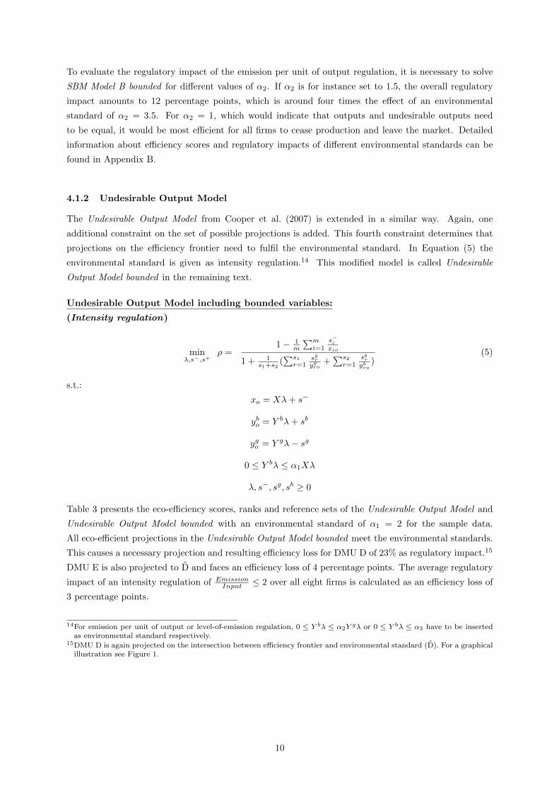
Undesirable Output Model including bounded variables:

(Intensity regulation)

minλ,s−,s+

ρ =1− 1

m

∑mi=1

s−ixio

1 + 1s1+s2

(∑s1r=1

sgrygro

+∑s2r=1

sbrybro

)(5)

s.t.:

xo = Xλ+ s−

ybo = Y bλ+ sb

ygo = Y gλ− sg

0 ≤ Y bλ ≤ α1Xλ

λ, s−, sg, sb ≥ 0

Table 3 presents the eco-efficiency scores, ranks and reference sets of the Undesirable Output Model and

Undesirable Output Model bounded with an environmental standard of α1 = 2 for the sample data.

All eco-efficient projections in the Undesirable Output Model bounded meet the environmental standards.

This causes a necessary projection and resulting efficiency loss for DMU D of 23% as regulatory impact.15

DMU E is also projected to D and faces an efficiency loss of 4 percentage points. The average regulatory

impact of an intensity regulation of EmissionInput ≤ 2 over all eight firms is calculated as an efficiency loss of

3 percentage points.

14For emission per unit of output or level-of-emission regulation, 0 ≤ Y bλ ≤ α2Y gλ or 0 ≤ Y bλ ≤ α3 have to be insertedas environmental standard respectively.

15DMU D is again projected on the intersection between efficiency frontier and environmental standard (D). For a graphicalillustration see Figure 1.

10

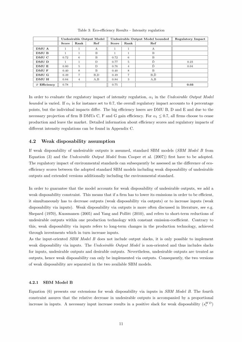
Table 3: Eco-efficiency Results – Intensity regulation

Undesirable Output Model Undesirable Output Model bounded Regulatory Impact

Score Rank Ref Score Rank Ref

DMU A 1 1 A 1 1 A

DMU B 1 1 B 1 1 B

DMU C 0.72 6 B 0.72 6 B

DMU D 1 1 D 0.77 5 D 0.23

DMU E 0.80 5 D 0.76 4 D 0.04

DMU F 0.40 8 B 0.40 8 B

DMU G 0.49 7 B,D 0.49 7 B,D

DMU H 0.84 4 A,B 0.84 3 A,B

∅ Efficiency 0.78 0.75 0.03

In order to evaluate the regulatory impact of intensity regulation, α1 in the Undesirable Output Model

bounded is varied. If α1 is for instance set to 0.7, the overall regulatory impact accounts to 4 percentage

points, but the individual impacts differ. The big efficiency losers are DMU B, D and E and due to the

necessary projection of firm B DMUs C, F and G gain efficiency. For α1 ≤ 0.7, all firms choose to cease

production and leave the market. Detailed information about efficiency scores and regulatory impacts of

different intensity regulations can be found in Appendix C.

4.2 Weak disposability assumption

If weak disposability of undesirable outputs is assumed, standard SBM models (SBM Model B from

Equation (3) and the Undesirable Output Model from Cooper et al. (2007)) first have to be adopted.

The regulatory impact of environmental standards can subsequently be assessed as the difference of eco-

efficiency scores between the adopted standard SBM models including weak disposability of undesirable

outputs and extended versions additionally including the environmental standard.

In order to guarantee that the model accounts for weak disposability of undesirable outputs, we add a

weak disposability constraint. This means that if a firm has to lower its emissions in order to be efficient,

it simultaneously has to decrease outputs (weak disposability via outputs) or to increase inputs (weak

disposability via inputs). Weak disposability via outputs is more often discussed in literature, see e.g.

Shepard (1970), Kuosmanen (2005) and Yang and Pollitt (2010), and refers to short-term reductions of

undesirable outputs within one production technology with constant emission-coefficient. Contrary to

this, weak disposability via inputs refers to long-term changes in the production technology, achieved

through investments which in turn increase inputs.

As the input-oriented SBM Model B does not include output slacks, it is only possible to implement

weak disposability via inputs. The Undesirable Output Model is non-oriented and thus includes slacks

for inputs, undesirable outputs and desirable outputs. Nevertheless, undesirable outputs are treated as

outputs, hence weak disposability can only be implemented via outputs. Consequently, the two versions

of weak disposability are separated in the two available SBM models.

4.2.1 SBM Model B

Equation (6) presents our extensions for weak disposability via inputs in SBM Model B. The fourth

constraint assures that the relative decrease in undesirable outputs is accompanied by a proportional

increase in inputs. A necessary input increase results in a positive slack for weak disposability (sWDr )

11

which enters the objective function.16 Any weak disposability slack will lower the efficiency of the

respective firm. This model is called SBM Model B weak in the remaining text.

SBM Model B including weak disposability via inputs:

minλ,s−,sb

ρ = 1− 1

m+ s2 + s2(

m∑i=1

s−ixio

+

s2∑r=1

sbrybro

+

s2∑i,r=1

sWDr

xio) (6)

s.t.:

xo = Xλ+ s−

ybo = Y bλ+ sb

ygo ≤ Y gλ

sbrybro

=sWDr

xio

λ, s−, sb, sWDr ≥ 0

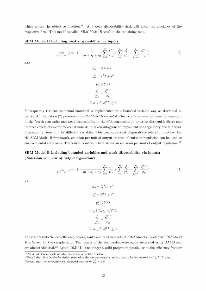
Subsequently the environmental standard is implemented in a bounded-variable way as described in

Section 4.1. Equation (7) presents the SBM Model B extended, which contains an environmental standard

in the fourth constraint and weak disposability in the fifth constraint. In order to distinguish direct and

indirect effects of environmental standards, it is advantageous to implement the regulatory and the weak

disposability constraint for different variables. This means, as weak disposability refers to inputs within

the SBM Model B framework, emission per unit of output or level-of-emission regulation can be used as

environmental standards. The fourth constraint here shows an emission per unit of output regulation.17

SBM Model B including bounded variables and weak disposability via inputs:

(Emission per unit of output regulation)

minλ,s−,sb

ρ = 1− 1

m+ s2 + s2(

m∑i=1

s−ixio

+

s2∑r=1

sbrybro

+

s2∑i,r=1

sWDr

xio) (7)

s.t.:

xo = Xλ+ s−

ybo = Y bλ+ sb

ygo ≤ Y gλ

0 ≤ Y bλ ≤ α2Ygλ

sbrybro

=sWDr

xio

λ, s−, sb, sWDr ≥ 0

Table 4 presents the eco-efficiency scores, ranks and reference sets of SBM Model B weak and SBM Model

B extended for the sample data. The results of the two models were again generated using GAMS and

are almost identical.18 Again, DMU D is no longer a valid projection possibility at the efficiency frontier

16As an additional slack variable enters the objective function,17Recall that for a level-of-emission regulation the environmental standard has to be formulated as 0 ≤ Y bλ ≤ α3.18Recall that the environmental standard was set to Y b

Y g ≤ 3.5.

12

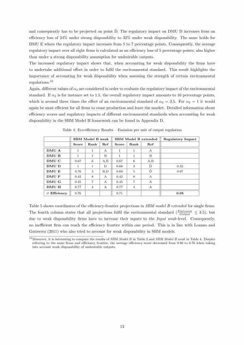
and consequently has to be projected on point D. The regulatory impact on DMU D increases from an

efficiency loss of 24% under strong disposability to 32% under weak disposability. The same holds for

DMU E where the regulatory impact increases from 5 to 7 percentage points. Consequently, the average

regulatory impact over all eight firms is calculated as an efficiency loss of 5 percentage points, also higher

than under a strong disposability assumption for undesirable outputs.

The increased regulatory impact shows that, when accounting for weak disposability the firms have

to undertake additional effort in order to fulfil the environmental standard. This result highlights the

importance of accounting for weak disposability when assessing the strength of certain environmental

regulations.19

Again, different values of α2 are considered in order to evaluate the regulatory impact of the environmental

standard. If α2 is for instance set to 1.5, the overall regulatory impact amounts to 16 percentage points,

which is around three times the effect of an environmental standard of α2 = 3.5. For α2 = 1 it would

again be most efficient for all firms to cease production and leave the market. Detailed information about

efficiency scores and regulatory impacts of different environmental standards when accounting for weak

disposability in the SBM Model B framework can be found in Appendix D.

Table 4: Eco-efficiency Results – Emission per unit of output regulation

SBM Model B weak SBM Model B extended Regulatory Impact

Score Rank Ref Score Rank Ref

DMU A 1 1 A 1 1 A

DMU B 1 1 B 1 1 B

DMU C 0.67 6 A,B 0.67 6 A,B

DMU D 1 1 D 0.68 3 D 0.32

DMU E 0.76 5 B,D 0.69 5 D 0.07

DMU F 0.42 8 A 0.42 8 A

DMU G 0.45 7 A 0.45 7 A

DMU H 0.77 4 A 0.77 4 A

∅ Efficiency 0.76 0.71 0.05

Table 5 shows coordinates of the efficiency-frontier projections in SBM model B extended for single firms.

The fourth column states that all projections fulfil the environmental standard (EmissionOutput ≤ 3.5), but

due to weak disposability firms have to increase their inputs to the Input weak -level. Consequently,

no inefficient firm can reach the efficiency frontier within one period. This is in line with Lozano and

Gutierrez (2011) who also tried to account for weak disposability in SBM models.

19Moreover, it is interesting to compare the results of SBM Model B in Table 2 and SBM Model B weak in Table 4. Despitereferring to the same firms and efficiency frontier, the average efficiency score decreased from 0.80 to 0.76 when takinginto account weak disposability of undesirable outputs.

13

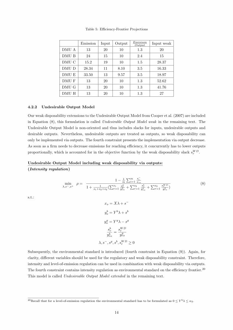
Table 5: Efficiency-Frontier Projections

Emission Input Output EmisisonOutput Input weak

DMU A 13 20 10 1.3 20

DMU B 24 15 10 2.4 15

DMU C 15.2 19 10 1.5 28.37

DMU D 28.34 11 8.10 3.5 16.33

DMU E 33.50 13 9.57 3.5 18.97

DMU F 13 20 10 1.3 52.62

DMU G 13 20 10 1.3 41.76

DMU H 13 20 10 1.3 27

4.2.2 Undesirable Output Model

Our weak disposability extensions to the Undesirable Output Model from Cooper et al. (2007) are included

in Equation (8), this formulation is called Undesirable Output Model weak in the remaining text. The

Undesirable Output Model is non-oriented and thus includes slacks for inputs, undesirable outputs and

desirable outputs. Nevertheless, undesirable outputs are treated as outputs, so weak disposability can

only be implemented via outputs. The fourth constraint presents the implementation via output decrease.

As soon as a firm needs to decrease emissions for reaching efficiency, it concurrently has to lower outputs

proportionally, which is accounted for in the objective function by the weak disposability slack sWDr .

Undesirable Output Model including weak disposability via outputs:

(Intensity regulation)

minλ,s−,s+

ρ =1− 1

m

∑mi=1

s−ixio

1 + 1s1+s2+s2

(∑s1r=1

sgrygro

+∑s2r=1

sbrybro

+∑s2r=1

sWDr

ygro)

(8)

s.t.:

xo = Xλ+ s−

ybo = Y bλ+ sb

ygo = Y gλ− sg

sbrybro

=sWDr

ygro

λ, s−, sg, sb, sWDr ≥ 0

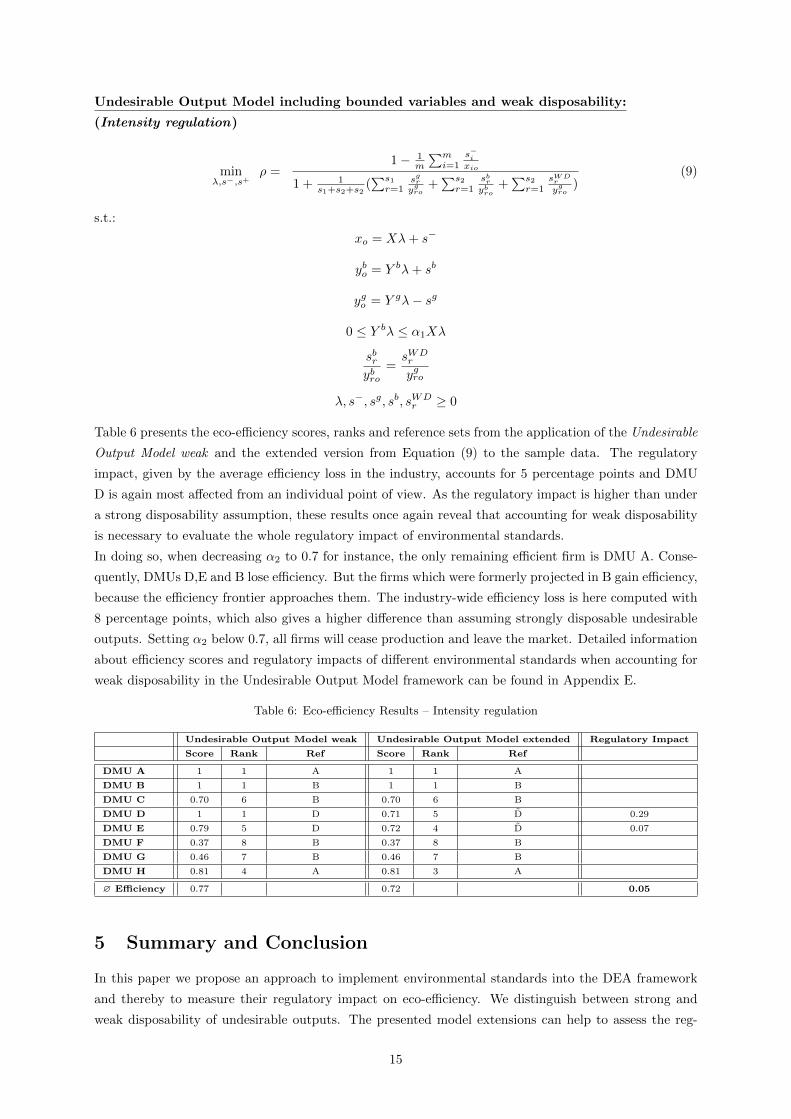
Subsequently, the environmental standard is introduced (fourth constraint in Equation (9)). Again, for

clarity, different variables should be used for the regulatory and weak disposability constraint. Therefore,

intensity and level-of-emission regulation can be used in combination with weak disposability via outputs.

The fourth constraint contains intensity regulation as environmental standard on the efficiency frontier.20

This model is called Undesireable Output Model extended in the remaining text.

20Recall that for a level-of-emission regulation the environmental standard has to be formulated as 0 ≤ Y bλ ≤ α3.

14

Undesirable Output Model including bounded variables and weak disposability:

(Intensity regulation)

minλ,s−,s+

ρ =1− 1

m

∑mi=1

s−ixio

1 + 1s1+s2+s2

(∑s1r=1

sgrygro

+∑s2r=1

sbrybro

+∑s2r=1

sWDr

ygro)

(9)

s.t.:

xo = Xλ+ s−

ybo = Y bλ+ sb

ygo = Y gλ− sg

0 ≤ Y bλ ≤ α1Xλ

sbrybro

=sWDr

ygro

λ, s−, sg, sb, sWDr ≥ 0

Table 6 presents the eco-efficiency scores, ranks and reference sets from the application of the Undesirable

Output Model weak and the extended version from Equation (9) to the sample data. The regulatory

impact, given by the average efficiency loss in the industry, accounts for 5 percentage points and DMU

D is again most affected from an individual point of view. As the regulatory impact is higher than under

a strong disposability assumption, these results once again reveal that accounting for weak disposability

is necessary to evaluate the whole regulatory impact of environmental standards.

In doing so, when decreasing α2 to 0.7 for instance, the only remaining efficient firm is DMU A. Conse-

quently, DMUs D,E and B lose efficiency. But the firms which were formerly projected in B gain efficiency,

because the efficiency frontier approaches them. The industry-wide efficiency loss is here computed with

8 percentage points, which also gives a higher difference than assuming strongly disposable undesirable

outputs. Setting α2 below 0.7, all firms will cease production and leave the market. Detailed information

about efficiency scores and regulatory impacts of different environmental standards when accounting for

weak disposability in the Undesirable Output Model framework can be found in Appendix E.

Table 6: Eco-efficiency Results – Intensity regulation

Undesirable Output Model weak Undesirable Output Model extended Regulatory Impact

Score Rank Ref Score Rank Ref

DMU A 1 1 A 1 1 A

DMU B 1 1 B 1 1 B

DMU C 0.70 6 B 0.70 6 B

DMU D 1 1 D 0.71 5 D 0.29

DMU E 0.79 5 D 0.72 4 D 0.07

DMU F 0.37 8 B 0.37 8 B

DMU G 0.46 7 B 0.46 7 B

DMU H 0.81 4 A 0.81 3 A

∅ Efficiency 0.77 0.72 0.05

5 Summary and Conclusion

In this paper we propose an approach to implement environmental standards into the DEA framework

and thereby to measure their regulatory impact on eco-efficiency. We distinguish between strong and

weak disposability of undesirable outputs. The presented model extensions can help to assess the reg-

15

ulatory impact of environmental standards in advance. By using an industry sample at one point in

time, regulators can compare the efficiency scores of the firms when applying a usual slack-based measure

(SBM) model and the extended counterpart to this sample. The difference in eco-efficiency scores can

be interpreted as regulatory impact of the environmental standard. The possibility to assess the regula-

tory impact in advance could provide support for environmental policy makers in choosing appropriate

instruments. Additionally, it should help to evaluate and adjust the intensity of regulation before taking

political action.

As one standard feature of basic DEA models (as e.g. CCR from Charnes et al. (1978)) lies in the

exogeneity of inputs, desirable and undesirable outputs and the optimisation over weights, it is not pos-

sible to introduce constraints for these parameters directly. Therefore, we implement the environmental

standard using a bounded variables framework which allows constraints on the efficiency frontier. The

regulatory impact of the environmental standard on a particular firm is determined by the comparison of

its eco-efficiency scores before and after fictive introduction of the standard. The regulatory impact for

the industry is measured by comparison of average eco-efficiencies. As we use an ex-ante approach, the

computed regulatory impact can be interpreted as a lower bound of the ex-post regulatory impact.

Assessing the regulatory impact is exclusively based on a comparison of eco-efficiency scores. For that

reason, a SBM framework, accounting for possible slacks, is more advantageous for our purpose. Two

possible models for measuring eco-efficiency are considered: a SBM version of Model B from Korhonen

and Luptacik (2004) and the Undesirable Output Model from Cooper et al. (2007). These models con-

stitute the starting point for the methodological implementation of an environmental standard into the

DEA framework. Moreover, we distinguish between weak and strong disposability of undesirable outputs

and develop corresponding models, where weak disposability itself is an extension to common SBM eco-

efficiency models.

Especially the great flexibility in our proposed model framework constitutes an advantage for regulatory

authorities and environmental policy makers. As the regulator can choose between two general SBM

model frameworks, three types of environmental standards and two weak disposability versions, the model

can be adopted to a wide range of industries. Moreover, assessing the regulatory impact of environmental

standards in advance can help choosing appropriate instruments and a reasonable intensity of regulation.

The application of our proposed method to assess the regulatory impact of environmental standards in

advance is interesting for different industries and offers large scope for further research. One interesting

example is for instance to assess which environmental standard would be most advantageous and effective

in reducing emissions in electricity generation.

16

APPENDICES

A Undesirable Output Model from Cooper et al. (2007)

minλ,s−,s+

ρ =1− 1

m

∑mi=1

s−ixio

1 + 1s1+s2

(∑s1r=1

sgrygro

+∑s2r=1

sbrybro

)(10)

s.t.:

xo = Xλ+ s−

ybo = Y bλ+ sb

ygo = Y gλ− sg

λ, s−, sg, sb,≥ 0

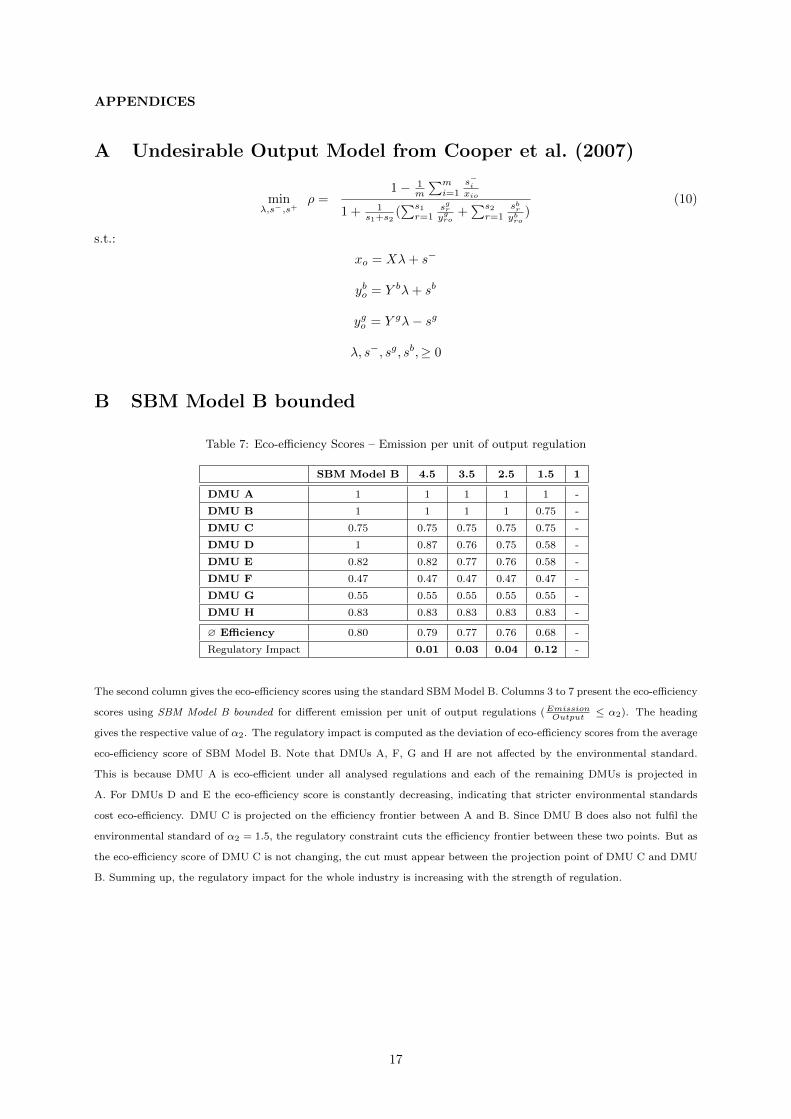
B SBM Model B bounded

Table 7: Eco-efficiency Scores – Emission per unit of output regulation

SBM Model B 4.5 3.5 2.5 1.5 1

DMU A 1 1 1 1 1 -

DMU B 1 1 1 1 0.75 -

DMU C 0.75 0.75 0.75 0.75 0.75 -

DMU D 1 0.87 0.76 0.75 0.58 -

DMU E 0.82 0.82 0.77 0.76 0.58 -

DMU F 0.47 0.47 0.47 0.47 0.47 -

DMU G 0.55 0.55 0.55 0.55 0.55 -

DMU H 0.83 0.83 0.83 0.83 0.83 -

∅ Efficiency 0.80 0.79 0.77 0.76 0.68 -

Regulatory Impact 0.01 0.03 0.04 0.12 -

The second column gives the eco-efficiency scores using the standard SBM Model B. Columns 3 to 7 present the eco-efficiency

scores using SBM Model B bounded for different emission per unit of output regulations (EmissionOutput

≤ α2). The heading

gives the respective value of α2. The regulatory impact is computed as the deviation of eco-efficiency scores from the average

eco-efficiency score of SBM Model B. Note that DMUs A, F, G and H are not affected by the environmental standard.

This is because DMU A is eco-efficient under all analysed regulations and each of the remaining DMUs is projected in

A. For DMUs D and E the eco-efficiency score is constantly decreasing, indicating that stricter environmental standards

cost eco-efficiency. DMU C is projected on the efficiency frontier between A and B. Since DMU B does also not fulfil the

environmental standard of α2 = 1.5, the regulatory constraint cuts the efficiency frontier between these two points. But as

the eco-efficiency score of DMU C is not changing, the cut must appear between the projection point of DMU C and DMU

B. Summing up, the regulatory impact for the whole industry is increasing with the strength of regulation.

17

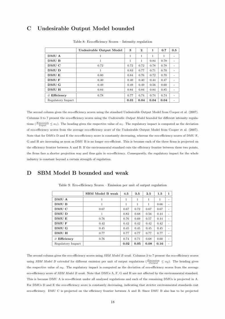
C Undesirable Output Model bounded

Table 8: Eco-efficiency Scores – Intensity regulation

Undesirable Output Model 3 2 1 0.7 0.5

DMU A 1 1 1 1 1 -

DMU B 1 1 1 0.84 0.78 -

DMU C 0.72 0.72 0.72 0.78 0.78 -

DMU D 1 0.83 0.77 0.71 0.70 -

DMU E 0.80 0.84 0.76 0.72 0.70 -

DMU F 0.40 0.40 0.40 0.44 0.47 -

DMU G 0.49 0.49 0.49 0.56 0.60 -

DMU H 0.84 0.84 0.84 0.84 0.85 -

∅ Efficiency 0.78 0.77 0.74 0.74 0.74 -

Regulatory Impact 0.01 0.04 0.04 0.04 -

The second column gives the eco-efficiency scores using the standard Undesirable Output Model from Cooper et al. (2007).

Columns 3 to 7 present the eco-efficiency scores using the Undesirable Output Model bounded for different intensity regula-

tions (EmissionInput

≤ α1). The heading gives the respective value of α1. The regulatory impact is computed as the deviation

of eco-efficiency scores from the average eco-efficiency score of the Undesirable Output Model from Cooper et al. (2007).

Note that for DMUs D and E the eco-efficiency score is constantly decreasing, whereas the eco-efficiency scores of DMU F,

G and H are increasing as soon as DMU B is no longer eco-efficient. This is because each of the three firms is projected on

the efficiency frontier between A and B. If the environmental standard cuts the efficiency frontier between these two points,

the firms face a shorter projection way and thus gain in eco-efficiency. Consequently, the regulatory impact for the whole

industry is constant beyond a certain strength of regulation.

D SBM Model B bounded and weak

Table 9: Eco-efficiency Scores – Emission per unit of output regulation

SBM Model B weak 4.5 3.5 2.5 1.5 1

DMU A 1 1 1 1 1 -

DMU B 1 1 1 1 0.66 -

DMU C 0.67 0.67 0.72 0.67 0.67 -

DMU D 1 0.82 0.68 0.56 0.44 -

DMU E 0.76 0.76 0.69 0.57 0.44 -

DMU F 0.42 0.42 0.42 0.42 0.42 -

DMU G 0.45 0.45 0.45 0.45 0.45 -

DMU H 0.77 0.77 0.77 0.77 0.77 -

∅ Efficiency 0.76 0.74 0.71 0.68 0.60 -

Regulatory Impact 0.02 0.05 0.08 0.16 -

The second column gives the eco-efficiency scores using SBM Model B weak. Columns 3 to 7 present the eco-efficiency scores

using SBM Model B extended for different emission per unit of output regulations (EmissionOutput

≤ α2). The heading gives

the respective value of α2. The regulatory impact is computed as the deviation of eco-efficiency scores from the average

eco-efficiency score of SBM Model B weak. Note that DMUs A, F, G and H are not affected by the environmental standard.

This is because DMU A is eco-efficient under all analysed regulations and each of the remaining DMUs is projected in A.

For DMUs D and E the eco-efficiency score is constantly decreasing, indicating that stricter environmental standards cost

eco-efficiency. DMU C is projected on the efficiency frontier between A and B. Since DMU B also has to be projected

18

for α2 = 1.5 the environmental standard cuts the efficiency frontier between A and B. More precisely, the variation in

eco-efficiency scores of DMU C indicates that the efficiency frontier is intersected between the projection point of DMU C

and DMU A. Summing up, the regulatory impact for the whole industry is increasing with strength of regulation on. Due

to the weak disposability assumption the eco-efficiency decrease is higher than under strong disposability of undesirable

outputs.

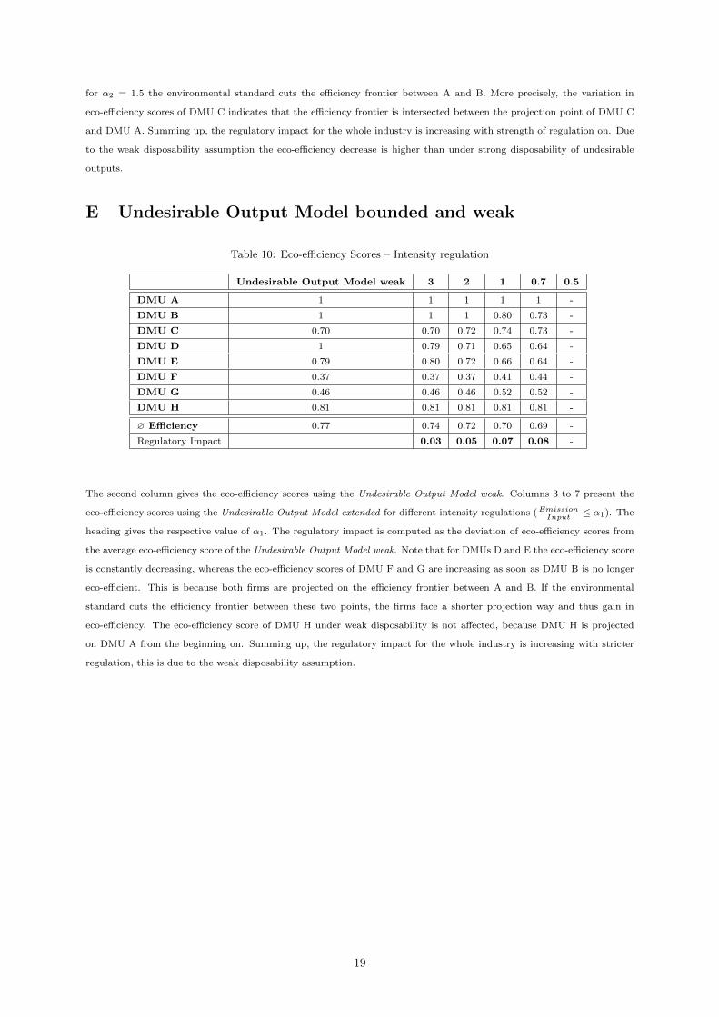
E Undesirable Output Model bounded and weak

Table 10: Eco-efficiency Scores – Intensity regulation

Undesirable Output Model weak 3 2 1 0.7 0.5

DMU A 1 1 1 1 1 -

DMU B 1 1 1 0.80 0.73 -

DMU C 0.70 0.70 0.72 0.74 0.73 -

DMU D 1 0.79 0.71 0.65 0.64 -

DMU E 0.79 0.80 0.72 0.66 0.64 -

DMU F 0.37 0.37 0.37 0.41 0.44 -

DMU G 0.46 0.46 0.46 0.52 0.52 -

DMU H 0.81 0.81 0.81 0.81 0.81 -

∅ Efficiency 0.77 0.74 0.72 0.70 0.69 -

Regulatory Impact 0.03 0.05 0.07 0.08 -

The second column gives the eco-efficiency scores using the Undesirable Output Model weak. Columns 3 to 7 present the

eco-efficiency scores using the Undesirable Output Model extended for different intensity regulations (EmissionInput

≤ α1). The

heading gives the respective value of α1. The regulatory impact is computed as the deviation of eco-efficiency scores from

the average eco-efficiency score of the Undesirable Output Model weak. Note that for DMUs D and E the eco-efficiency score

is constantly decreasing, whereas the eco-efficiency scores of DMU F and G are increasing as soon as DMU B is no longer

eco-efficient. This is because both firms are projected on the efficiency frontier between A and B. If the environmental

standard cuts the efficiency frontier between these two points, the firms face a shorter projection way and thus gain in

eco-efficiency. The eco-efficiency score of DMU H under weak disposability is not affected, because DMU H is projected

on DMU A from the beginning on. Summing up, the regulatory impact for the whole industry is increasing with stricter

regulation, this is due to the weak disposability assumption.

19

References

Ali, A. and Seliford, L. (1990). Translation invariance in data envelopment analysis. Operations research

letters, 9, 403–405.

Charnes, A., Cooper, W., and Rhodes, E. (1978). Measuring efficiency of decision making units. European

Journal of Operational Research, 2, 429–444.

Cooper, W. W., Seiford, L. M., and Tone, K. (2007). Data Envelopment Analysis: A Comprehensive

Text With Models, Applications, References And DEA–Solver Software (2nd Edition). Springer, New

York.

Cropper, M. and Oates, W. (1992). Environmental economics: A survey. Journal of Economic Literature,

30, 675–740.

Dudenhoffer, F. (1984). The regulation of intensities and productivities: Concepts in environmental

policy. Journal of Institutional and Theoretical Economics, 140, 276–287.

Dyson, R., Allen, R., Camanho, A., Podinovski, V., Sarrico, C., and Shale, E. (2001). Pitfalls and

protocols in DEA. European Journal of Operational Research, 132, 245–259.

Forsund, F. R. (2008). Good modelling of bad outputs: Pollution and multiple-output production.

Memorandum, Department of Economics, University of Oslo.

Fare, R. and Grosskopf, S. (2003). Nonparametric productivity analysis with undesirable outputs: Com-

ment. American Journal of Agricultural Economics, 85, 1070–1074.

Fare, R. and Grosskopf, S. (2004). Modeling undesirable factors in efficiency evaluation: Comment.

European Journal of Operational Research, 157, 242–245.

Fare, R. and Grosskopf, S. (2009). A comment on weak disposability in nonparametric production

analysis. American Journal of Agricultural Economics, 91, 535–538.

Fare, R., Grosskopf, S., Lovell, K., and C.Pasurka (1989). Multilateral productivity comparisons when

some outputs are undesirable: a nonparametric approach. The Review of Economics and Statistics,

71(1), 90–98.

Fare, R., Grosskopf, S., and Pasurka, C. (1986). Effects on Relative Efficiency in Electric Power Gener-

ation due to Environmental Controls. Resources and Energy, 8, 167–184.

Fare, R. and Logan, J. (1983). The Rate-of-Return Regulated Firm: Cost and Production Duality. The

Bell Journal of Economics, 14(2), 405–414.

Fare, R. and Logan, J. (1992). The rate of return regulated version of Farrell efficiency. International

Journal of Production Economics, 27, 161–165.

Golany, B. and Roll, Y. (1989). An application procedure for DEA. Omega: The International Journal

of Management Science, 17, 237–250.

Golany, B. and Roll, Y. (1994). Incorporating standards via DEA. In A. Charnes, W. W. Cooper, A. Y.

Lewin, and L. M. Seiford (Eds.), Data envelopment analysis: Theory, methodology, and applications

(pp. 313–328). Kluwer, Boston.

20

Hailu, A. (2003). Nonparametric productivity analysis with undesirable outputs: Reply. American

Journal of Agricultural Economics, 85, 1075–1077.

Hailu, A. and Veeman, T. (2001). Non-parametric productivity analysis with undesirable outputs: An

application to the Canadian pulp and paper industry. American Journal of Agricultural Economics,

83, 605–616.

Helfand, G. (1991). Standards versus standards: the effects of different pollution restrictions. American

Economic Review, 81(3), 622–634.

Koopmans, T. (1951). Analysis of production as an efficient combination of activities. In T. Koopmans

(Ed.), Activity Analysis of Production and Allocation (pp. 33–97). Wiley, New York.

Korhonen, P. and Luptacik, M. (2004). Eco–efficiency analysis of power plants: An extension of data

envelopment analysis. European Journal of Operational Research, 154, 437–446.

Kuosmanen, T. (2005). Weak disposability in nonparametric production analysis with undesirable out-

puts. American Journal of Agricultural Economics, 87(4), 1077–1082.

Lozano, S. and Gutierrez, E. (2011). Slack–based measure of efficiency of airports with airplanes delays

as undesirable outputs. Computers and Operations Research, 38, 131–139.

Luptacik, M. (2009). Mathematical Optimization and Economic Analysis. Springer, New York.

Ouellette, P., Quesnel, J.-P., and Vigeant, S. (2009). Measuring Returns to Scale in DEA Models when

the Firm is Regulated. http://www.wise.xmu.edu.cn/Master/News/NewsPic/201063092839104.pdf.

Ouellette, P. and Vigeant, S. (2001). On the Existence of a Regulated Production Function. Journal of

Economics, 73(2), 193–200.

Podinovski, V. V. and Kuosmanen, T. (2011). Modelling weak disposability in data envelopment analysis

under relaxed convexity assumptions. European Journal of Operational Research, 211(3), 577–585.

Sahoo, B., Luptacik, M., and Mahlberg, B. (2011). Alternative measures of environmental technology

structure in dea: An application. European Journal of Operational Research, 215, 750–762.

Scheel, H. (2001). Undesirable outputs in efficiency evaluations. uropean Journal of Operational Research,

132, 400–410.

Shannon, C. (1997). Increasing Returns in Infinite–Horizon Economies. Review of Economic Studies, 64,

73–96.

Shepard, R. (1970). Theory of Cost and Production Functions. Princeton University Press.

Tyteca, D. (1996). On the measurement of the environmental performance of firms — a literature review

and a productive efficiency perspective. Journal of Environmental Management, 46, 281–308.

Yang, H. and Pollitt, M. (2010). The necessity of distinguishing weak and strong disposability among

undesirable outputs in DEA: Environmental performance of Chinese coal–fired power plants. Energy

Policy, 38, 4440–4444.

Zhou, P., Ang, B., and Poh, K. (2008). A survey of data envelopment analysis in energy and environmental

studies. European Journal of Operational Research, 189, 1–18.

Zofio, J. L. and Prieto, A. M. (2001). Environmental efficiency and regulatory standards: the case of

CO2 emissions from OECD industries. Resource and Energy Economics, 23, 63–83.

21