Eprints Cover Sheeteprints.qut.edu.au/2028/1/2028_2.pdf · Tests of the three issues require that measures be obtained for ... Whilst it is arguable that abnormal items are transitory

COVER SHEET

Author-version of article published as: Percy, Majella and Stokes, Donald J. (1992) Further Evidence on Empirical Relationships Between Earnings and Cash Flows. Accounting and Finance 32(1):pp. 27-50. Copyright 1992 Blackwell Publishing.

1

FURTHER EVIDENCE ON EMPIRICAL RELATIONSHIPS BETWEEN EARNINGS AND CASH FLOWS.

by

Majella Percy Queensland University of Technology and Donald J. Stokes University of Southern Queensland

Abstract:

Recently in Australia, regulations have been proclaimed requiring companies to make cashflow disclosures in addition to earnings disclosures from 30 June 1992. This paper provides evidence on relationships between earnings and cash flow measures and in so doing examines the external validity of a U.S.A. study of these relationships by Bowen. Burgstahler and Daley [1986]. We also extend their study through an industry analysis of the relationships. Evidence is presented first that shows low correlations between traditional cash flow measures (ie. net income plus depreciation and amortisation; and working capital from operations) and a more refined cash flow measure (with additional adjustments for changes in noncash current assets and current liabilities). Second, traditional cash flow measures exhibit high correlations with earnings, while the more refined cash flow measure has a lower correlation with earnings. Finally, traditional cash flow measures better predict future cash flows than models based on earnings or a more refined cash flow measure. The industry evidence, albeit on small sample sizes, shows that the results on the first two issues, but not the latter issue, are generalisable across industry categories.

Acknowledgements:

The authors acknowledge the comments and suggestions of Mike Bradbury and an anonymous referee together with colleagues at the University of Queensland and Queensland University of Technology, in particular Jennie Adams, Keitha Dunstan, Jere Francis, Don Hamson and Ian Zimmer.

2

1. Introduction

Recent research in the USA by Bowen, Burgstahler and Daley [1986] – hereafter BB&D [1986] – into the relationships between earnings and cash flows measures, demonstrated:

(1) Traditional measures of cash flow (ie net income plus depreciation and amortisation: and working capital from operations) are highly correlated with earnings, while more refined measures of cash flow have lower correlations with earnings;

(2) Earnings do not provide better forecasts of future cash flows than do cash flow measures.

Evidence of these relationships is of particular importance for models of firm valuation which use earnings as proxy measures for future cash flows and for assessments of business solvency which rely upon estimates of future cash flows available to settle obligations. Moreover, the evidence takes on added significance as there are new regulations in Australia requiring cash flow statements for financial reports produced for the year to 30 June 1992 and thereafter. The Australian Accounting Standards Board (AASB) issued Accounting Standard AASB 1026: Statement of Cash Flows in December 1991. AASB 1026 requires companies to report their cash flows for the financial year in order to provide information about a company’s operating and other activities (normally, financing and investing activities) for the financial year. The standard does not mandate which individual cash flow items fall into these three categories. The requirements of the Australian cash flow standard are similar to those contained in the United States (US) standard. The major difference is that US companies are allowed to assess cash flows using either the direct or indirect method, but Australian companies must report cash flows from operating activities calculated by use of the direct method, whereby cash inflows and cash outflows are presented in gross quantities. The Australian Stock Exchange has amended its Listing Rules to require half yearly and yearly cash flow statements for the period ended 30 June 1992 and thereafter.

This paper reports the results of a study which investigates the relationships between earnings and certain cash flow measures for Australian companies. Three specific issues examined by BB&D [1986] are considered:

I1 The correlation between traditional cash flow measures [ie (i) net income plus depreciation and amortisation and (ii) working capital from operations] and a refined measure of cash flow [with additional adjustments for changes in noncash current assets and current liabilities]

I2 The correlation between earnings and cash flow measures.

I3 The prediction of future cash flows using earnings and cash flow measures.

The study therefore examines the external validity of BB&D’s [1986] results. However, we also extend BB&D’s [1986] study via industry analysis of these issues using the Australian data. BB&D [1986] did not address the question of whether the results on issues I1 to I3 are generalisable across industry groups of companies. Recent research (e.g. Foster [1986, p.561], Bernard and Ruland [1987], Lobo and Song [1989]) suggests the possibility that cash flow information may provide differential information from earnings in valuation decisions and assessments of business solvency for some industries. The interpretation of differences between earnings and cash flows measures depends, e.g. upon inventory valuation methods used to calculate the former and on rates of inventory turnover. These factors tend to vary by industry. The focus on an industry analysis parallels the relevance

3

of economic context in examining the relationships between accounting and market based variables (see eg Bernard and Stober [1989], Antle, Demski and Ryan [1989]).

The paper is structured with the research design in section 2, the results in section 3, and conclusions in section 4.

2. Research Design

Tests of the three issues require that measures be obtained for earnings, traditional cash flows and refined cash flows. We use, where possible, the variable names and measures used by BB&D [1986] to facilitate comparisons across the studies. The earnings measure used is net income before extraordinary items (NIBEI). This measure is taken from the Australian Graduate School of Management (AGSM) Annual Report File:

Profit Reported (Variable 15) – Extraordinary Income (Variable 124) + Extraordinary Expenses (Variable 135)

Whilst it is arguable that abnormal items are transitory earnings components like extraordinary items, we do not adjust the NIBEI measures for abnormal items 1 . This is consistent with BB&D [1986]. Adjustments for abnormal items are made in two cash flow measures discussed below.

Two traditional cash flow measures are used. They require only a few adjustments to the earnings figure and follow the adjustments used by BB&D [1986, p. 715] for their traditional cash flow measures. The first is NIBEI plus depreciation and amortisation (NIDPR):

NIDPR = NIBEI DPR

Where DPR = Depreciation and amortisation changes (AGSM Report File Variables 125 + 126 + 127)

The second measure is working capital from operations (WCFO):

WCFO = NIDPR – ABN

Where ABN = adjustments for other elements of NIBEI not affecting working capital.

The ABN measure is taken from the AGSM Report File:

Profit on sale of fixed assets (I21) + Profit on sale of Investments (I22) + Abnormal income (I23) – Loss on Sale of fixed assets (I32) – Loss on sale of investments (I33) – Abnormal expenses (I34) – Change in deferred tax liability (I39)

Only one of the three refined cash flow measures used by BB&D [1986] is utilised here. 2

CFO = WCFO rREC rINV rOCA + rAP + rAP +rOCL

Where rREC = Changes in accounts receivable during the period. rINV = Changes in inventories during the period. rOCA = Changes in other current assets during the period.

1 In a preliminary analysis of the data, we included extraordinary items in NIBEI (consistent with the treatment of the abnormal items) i.e. NIBEI was set equal to the Profit Reported. Results are consistent with those reported below.

2 Neither the AGSM Annual Report File nor the annual reports of the companies in our sample provide the disclosures needed for the other two measures used by BB&D [1986].

4

rAP = Changes in accounts payable during the period. rTP = Changes in taxes payable during the period. rOCL = Changes in other current liabilities during the period.

Measures on these variables were collected for all firms on the AGSM Annual Report File for the last 12 years of available data held on the File. These are the years 1974 to 1985, a period comparable to that used by BB&D [1986]. There were 187 companies with 12 years annual report data on the File. However, 61 companies were missing one or more items required for the measures and these companies were deleted from the sample. A further 19 companies changed their balance dates during this period and their elimination left a final sample size of 107 companies.

For the industry analysis of the issues the 107 companies were classified into industry categories using the 1985 Australian Stock Exchange Industry groupings. Only 8 companies changed industry categories between 1974 and 1985 and these companies were excluded in the industry analysis. The distribution of the 99 companies across the categories is shown in Table 1.

BB&D [1986] used first differences [Xt+n – Xt+n1] and percentage change [Xt+n – Xt+n1/ Xt+n1] measures on the variables to overcome nonstationarity problems in the time series for the levels of the variables. Both first differences and percentage change time series are analysed in the tests below. All three issues 1113 are investigated on the pooled sample of 107 companies. The industry analysis described below is restricted to a subset of industry categories.

5

TABLE 1: Sample Companies by Industry Categories

_____________________________________________________________________ Industry ‘n’

_____________________________________________________________________ Heavy Engineering 14 Building Materials 12 Retail 9 Developers and Contractors 6 Food and Household Goods 5 Media 4 Automotive 4 Chemicals 4 Transport 3 Solid Fuels 2 Oil and Gas 2 Diversified Resources 2 Light Engineering 2 Paper and Packaging 2 Metals 1 Electrical & Household Durables 1 Alcohol and Tobacco 1 Textiles and Clothing 1 Banks and Finance 1 Insurance 1 Merchants and Agents 1 Other Services 9 Diversified and Miscellaneous 12

____ 99

___________________________________________________________________

3. Results

3.1 Pooled Analysis

This section reports the results on issues 1113 for the pooled sample of 107 companies identified in section 2.

3.1.1 Correlations Between Alternative Measures of Cash Flow: 11

Issue 11 investigates correlations between traditional cash flow measures (NIDPR, WCFO) and the refined measure of cash flow (CFO). For comparison with BB&D [1986], the correlation coefficients are squared and summary information on the distribution of each time series of R 2 across the firms by quintile 3 , together with the mean and median R 2 , are shown in Tables 2A and 2B. Table 2A reports the squared Pearson correlations and Table 2B the squared Spearman Rank correlations. The tables show that the median and mean squared correlations of the refined cash flow measure (CFO) with the more traditional cash flow measures (NIDPR and WCFO) are low for both the first differences and percentage change series.

3 Quintiles are scores corresponding to the percentile rank of 20, 40, 60 and 80. Thus the 20% Quintile shows the 21 st lowest correlation in the sorted correlation file for each variable.

6

TABLE 2A: Distribution of Squared Pearson Correlations (R 2 ) Between Earnings and Cash Flows Across Sample Firms

________________________________________________________________________________________ Variables in No of Quintiles Correlation* Insig 20% 40% 60% 80% Median Mean

R 2 ** (n=107)

Panel A: First Differences

Issue I1: (CFO, NIDPR) 73 .015 .092 .207 .473 .149 .243 (CFO, WCFO) 68 .018 .132 .290 .555 .201 .286

Issue 12: (NIDPR, NIBEI) 10 .757 .942 .976 .990 .958 .833 (WCFO, NIBEI) 37 .143 .394 .667 .850 .559 .521 (CFO, NIBEI) 70 .013 .051 .254 .493 .116 .247

Panel B: Percentage Changes

Issue 11: (CFO, NIDPR) 87 .014 .054 .127 .296 .099 .177 (CFO, WCFO) 81 .011 .055 .145 .423 .096 .219

Issue 12: (NIDPR, NIBEI) 15 .586 .860 .949 .983 .914 .772 (WCFO, NIBEI) 42 .074 .444 .649 .819 .554 .490 (CFO, NIBEI) 82 .011 .052 .126 .360 .087 .195 _______________________________________________________________________________________

* NIBEI = operating profit before extraordinary items NIDPR = operating profit plus depreciation and amortisation WCFO = working capital from operations CFO = cash flow from operations

** Number of firms (out of 107) for which the correlation is not statistically significant at the .05 level (using a twotailed test).

In Table 2A, for the first difference and percentage change series, between 19 and 36 percent of the 107 correlations are statistically significant at the .05 level. 4 The results in Table 2B are very similar to those in Table 2A. BB&D [1986] similarly obtained between 17 and 27 percent of the 324 correlations statistically significant at the .05 level. The results suggest that the more traditional measures of cash flow used in prior research are poor proxies for a more refined measure of cash flow incorporating additional adjustments.

4 Using first differences, 73 of the 107 correlations for (CFO, NIDPR) are insignificant – leaving 34 (32%) significant – and 68 of the 107 correlations for (CFO,WCFO) are insignificant – leaving 41 (36%) significant. Using percentage changes, 87 of the 107 correlations for (CFO, NIDPR) are insignificant – leaving 20 (19%) significant – and 81 of the 107 correlations for (CFO, WCFO) are insignificant – leaving 26 (24%) significant.

7

TABLE 2B: Distribution of Squared Spearman Rank Correlations (R 2 ) Between Earnings and Cash Flows Across sample Firms

________________________________________________________________________________________ Variables in No of Quintiles Correlation* Insig 20% 40% 60% 80% Median Mean

R 2 ** (n=107)


Issue I1: (CFO, NIDPR) 82 .006 .027 .111 .346 .056 .172 (CFO, WCFO) 82 .013 .072 .146 .405 .111 .192

Issue 12: (NIDPR, NIBEI) 13 .611 .838 .929 .976 .905 .772 (WCFO, NIBEI) 43 .096 .318 .556 .860 .421 .470 (CFO, NIBEI) 84 .008 .031 .119 .405 .050 .183


Issue 11: (CFO, NIDPR) 88 .016 .050 .111 .291 .068 .154 (CFO, WCFO) 86 .013 .056 .155 .318 .096 .167

Issue 12: (NIDPR, NIBEI) 15 .503 .815 .905 .952 .883 .744 (WCFO, NIBEI) 42 .111 .360 .592 .794 .421 .453 (CFO, NIBEI) 88 .016 .056 .137 .291 .096 .163 _______________________________________________________________________________________

*NIBEI = operating profit before extraordinary items NIDPR = operating profit plus depreciation and amortisation WCFO = working capital from operations CFO = cash flow from operations

**Number of firms (out of 107) for which the correlation is not statistically significant at the .05 level (using a twotailed test).

3.1.2 Correlations between Cash Flows and Earnings: I2

Tables 2A and 2B also reports the R 2 between the cash flow measures (NIDPR, WCFO, CFO) and earnings (NIBEI). The correlations of the refined measure of cash flow (CFO) with earnings (NIBEI) are lower than the correlations of traditional measures of cash flow (NIDPR and WCFO) with earnings (NIBEI). Once again these results are very similar to those on the equivalent BB&D correlations, and suggest that the correlations of the traditional measures of cash flow with earnings are notably greater than either the correlations of the traditional measures of cash flow with refined measures of cash flow, or the correlations of the refined measures of cash flow with earnings. These results are consistent with NIDPR and WCFO being comparable to earnings for most firms while the refined measure of cash flow (CFO) is distinct from earnings for most firms.

8

3.1.3 Predicting Cash Flows: I3

Following BB&D [1986], we investigate issue I3 using simple prediction models of the form:

Ŷi,t+1=Xi,t

Ŷi,t+2=Xi,t

Where Ŷi,t+1 = the forecast of the cash flow (CF) variable for firm ‘I’ in period ‘t+1’ Ŷi,t+2 = the forecast of the cash flow (CF) variable for firm ‘I’ in period ‘t+2’ Xi,t = the value of the predictor variable for firm ‘I’ in period ‘t’

The median absolute forecast error of each forecasted series was scaled by the actual value of the forecasted series in order to standardise the error terms. These forecast errors are reported in Table 3. The median is used as the measure of central tendency because the distributions of forecast errors were found to be skewed. 5 Panel A (B) contains the one (two) period ahead forecast errors. The diagonal contains the results of the random walk prediction models. A random walk earnings model (i.e., using this period’s NIBEI to predict one (two) period(s) ahead NIBEI) is displayed as a benchmark in the upper left cell of each panel in Table 3. The results are consistent with BB&D [1986]. The results show that the magnitudes of median relative forecast errors for random walk predictions of NIDPR and WCFO are smaller than for NIBEI, while the median relative forecast errors for random walk predictions of CFO are larger than for NIBEI.

Forecasts of one or twoperiodsahead NIDPR and WCFO have lower median percentage forecast errors than do forecasts of NIBEI. This suggests that traditional measures of cash flow may be more predictable than earnings. In contrast, it can be seen from the table that the refined measure of cash flow, CFO, is more difficult to predict than earnings. 6

These results are consistent with BB&D’s [1986] results.

The average rank of the median absolute forecast errors across years is also presented in Table 3 as another summary measure of the results. To calculate this average rank we followed BB&D’s [1986, pp. 721722] procedure. Absolute forecast errors were first segregated by year. The median absolute forecast error of each predictor variable was then assigned a rank within each year and the ranks on each predictor variable were averaged across the years. The ranks provide additional information about the distribution of the forecast errors across years. An average rank of 1.0 indicates that the predictor variable had the lowest median absolute forecast error in each of the ten years. The results in Table 3 support the conclusions that, for all cash flow variables except CFO, a random walk model performs at least as well and usually better than, predictions based on variables with fewer adjustments in moving from NIBEI to CFO.

5 The mean absolute forecast errors ranged from 2 to 57 times larger than the median values, BB&D [1986, p. 721] report their mean absolute forecast errors were often twice as high as the median values. 6 BB&D suggest (p. 721) this is evidence of income smoothing being a feature of the accrual process.

9

TABLE 3: Medians (and Average Ranks) *of Absolute Forecast Errors Scaled by the Actual Value of the Forecasted Series

___________________________________________________________________________________

Dependent Predictor Variables Variables NIBEI NIDPR WCFO CFO ___________________________________________________________________________________ Panel A: One Period Ahead Forecasts

NIBEI** .236 ()

NIDPR .407 .193 (2.0) (1.0)

WCFO .394 .187 .192 (3.0) (1.2) (1.8)

CFO .600 .518 .506 .715 (2.5) (2.0) (1.9) (3.60)

Panel B: Two Period Ahead Forecasts

NIBEI** .390 ()

NIDPR .533 .327 (2.0) (1.0)

WCFO .502 .307 .320 (3.0) (1.33) (1.67)

CFO .694 .636 .617 .817 (3.11) (1.67) (1.44) (3.78)

___________________________________________________________________________________ * Ranks based on the median forecast error across predictor variables in a given year are

averaged across ten years in Panel A or nine years in Panel B. * A random walk model of NIBEI is presented as a benchmark.

TABLE 4: Friedman Tests* of the Null Hypothesis that, for each Cash Flow Variable, Median Forecast Errors are Equal Across all Single Predictor Models**

___________________________________________________________________________________ One Period Ahead Two Periods Ahead

CF Variable ChiSq. Signif. ChiSq. Signif. (Twotailed) (TwoTailed)

NIDPR 10.000 ,0016 9.000 .0027

WCFO 16.800 .0002 14.0000 .0009

CFO 10.920 .0122 20.600 .0001 ___________________________________________________________________________________ * Friedman’s twoway analysis of variance by ranks (Siegel (1956.p. 166)). ** For example, for CFO, the null hypothesis is that median forecast errors are equal

across single predictor models based on NIBEL, NIDPR, WCFO or CFO. The hypothesis is rejected if any of the single predictor models is detectably better or worse.

10

The statistical significance of the differences in the median absolute forecast errors for each cash flow variable is examined in Table 4 using the Friedman twoway analysis of variance by ranks (Siegel, 1956.p.166). For each of the three predicted variables, the results indicate some predictors perform significantly better than others at the .01 level. The result here again are very similar to BB&D (1986, pp. 726722).

The statistical significance of the individual pairwise differences was evaluated using Sign test(Siegel (1956. p.68) and these results are reported in Table 5. Column four shows this period’s NIDPR better predicts one – and twoperiodsahead NIDPR than does NIBEI, whereas NIDPR and WCFO are consistently the better predictors (at the .05 level, one tailed) of CFO – both one and twoperiodsahead. BB&D (1986. pp. 733723) results are consistent with these, but in addition they found that WCFO better predicts one and two periodsahead WCFO than does NIBEI or NIDPR. There are no obvious reasons for this apparent inconsistency.

Since Table 5 shows random walk models perform at least as well as others, if either of the traditional measures of cash flow (NIDPR or WCFO) is the relevant measure of cash flow, then historical cash flow variables better predict future cash flows. However, in many decisions, the relevant cash flow variable may be closer to a refined measure of cash flow. The results for predictions of CFO are not as clear. For CFO, the Sign tests reported in Table 5 indicate that the traditional cash flow measures (WCFO and NIDPR) provide significantly better forecasts of one and twoperiodsahead CFO than does last period’s CFO. However, NIBEI did not perform significantly better the CFO in forecasts of one and twoperiodsahead CFO.

TABLE 5: Pairwise Sign Tests of the Null Hypothesis that the Median Forecast Error Using predictor ‘X1’ is Equal to the Median Forecast Error Using ‘X2’*

___________________________________________________________________________________ Predictor with Lower Significance Level

“CF” Median (Onetailed) Variable Predicators Considered Absolute Predicted Forecast Periods Ahead

‘X1’ ‘X2’ Error One Two ___________________________________________________________________________________ NIDPR NIDPR NIBEI NIDPR .002 .0039

WCFO WCFO NIDPR NIDPR .1094 .5078 WCFO WCFO NIBEI WCFO .002 .0039 WCFO NIDPR NIBEI NIDPR .002 .0039

CFO CFO WCFO WCFO .0215 .0039 CFO CFO NIDPR NIDPR .0215 .0039 CFO CFO NIBEI NIBEI .1094 .1797 CFO WCFO NIDPR 1.000 1.000 CFO WCFO NIBEI WCFO .3437 .0039 CFO NIDPR NIBEI NIDPR .7539 .0391 ___________________________________________________________________________________

*The alternative hypothesis is that the median forecast error using ‘X1’ is not equal to the median forecast error using ‘X2’. Column 4 lists the predictor that results in the lower forecast error for both one and two periods ahead. For example, when predicting future CFO using historical CFO versus WCFO, we can reject the null in favour of WCFO being a better predictor of future CFO (one and twoperiodsahead) than is past CFO.

11

3.2 Industry Analysis

This section reports the results of an industry analysis of issues 1113. An examination of the distributions of R 2 reported in Tables 2A and 2B suggests outlier values of the R 2 are concentrated in the Developers and Contractors, heavy Engineering and Retail industries. The industry analysis is completed on these three industries as well as the Building and Materials industry which has a comparable sample size of firms. 7 However, the results must be interpreted with some caution given the small sample sizes for the industry categories

3.2.1 Industry Correlations between Alternative Measures of Cash Flow: 11

Issue 11 focuses upon the correlations between the traditional cash flow measures (NIDPR, WCFO) and the refined measure of cash flow (CFO). The mean and median of each time series of Pearson R 2 for industry categories containing at least 6 companies, are reported in Table 6. They show that across the industries the squared correlations are low for both the first difference and percentage change series. This is consistent with the pooled sample results in Table 2A.

3.2.2 Industry Correlations Between Cash Flows and Earnings: 12

Issue 12 deals with the correlations between the cash flow measures (NIDPR, WCFO, CFO) and earnings (NIBEI). The results on the issue for the industry categories are also reported in Table 6. For both first differences and percentage changes, the squared Pearson correlations between the refined measure of cash flow (CFO) with earnings (NIBEI) are lower in each industry that the correlations of traditional measures of cash flow (NIDPR and WCFO) with earnings (NIBEI). This pattern was in evidence in the pooled sample results in Table 2A.

In addition, across industries, there is some suggestion of differences in the median squared correlations of CFO and NIBEI. In particular the Developers and Contractors, Heavy Engineering and the Retail industries exhibit lower median squared correlations. The mean squared correlations exhibit a similar, though less pronounced pattern, across the industries. However, the proportion of insignificant squared correlations exhibits less disparity across the industries.

3.2.3 Industry Predictions of Cash Flows: 13

Issue 13 addresses the prediction of future cash flows using earnings and cash flow measures. The results on this issue for the four industry categories used in Table 6 are reported in tables contained in the Appendix. Generally, the results for each industry are consistent with those shown for the pooled sample in Tables 3, 4 and 5, with the following exceptions: (i) With Developers and Contractors and Heavy Engineering firms, there are larger

errors in CFO predictions (both one and twoperiods ahead CFO) using all four predictor variable. However, there are no significant differences in the median absolute forecast errors using the four predictor variables.

(ii) Firms in the Building Materials industry have smaller CFO prediction errors for both one and twoperiods ahead using all four predictor variables. However, the traditional cash flow measures do not provide significantly better forecasts of both one and two periods ahead CFO than does last periods’s CFO.

(iii) Firms in the Retail industry have smaller CFO prediction errors for both one and two periods ahead using all four predictor variables.

7 The “Other Services” and “Diversified and Miscellaneous” categories of comparable size were ignored because of the diverse nature of the categories

12

TABLE 6 : Distributions of Squared Pearson Correlations (R 2 ) Between Earnings and Cash Flows by Industries

________________________________________________________________________________________ Developers Building Heavy Retail Total

& Materials Engineering Sample Contractors (From

Table 2A)

No Firms 6 12 14 9 107


Issue I1: Median .006 .174 .050 .042 .149 (CFO, NIDPR) Mean .110 .266 .227 .158 .243

No.Insig.R 2 5 8 11 6 73

Median .124 .354 .126 .151 .201 (CFO, WCFO) Mean .158 .384 .297 .204 .286

No.Insig.R 2 5 6 9 7 68

Issue 12 Median .965 .954 .978 .984 .958 (NIDPR, NIBEI) Mean .890 .898 .911 .944 .833

No.Insig.R 2 0 0 0 0 10

Median .565 .559 .843 .628 .559 (WCFO, NIBEI) Mean .481 .520 .772 .463 .521

No.Insig.R 2 2 4 1 3 37

Median .033 .321 .030 .030 .116 (CFO, NIBEI) Mean .174 .326 .215 .157 .247

No.Insig.R 2 4 7 11 6 70


Issue 11: Median .056 .082 .077 .120 .099 (CFO, NIDPR) Mean .060 .159 .145 .142 .177

No.Insig.R 2 6 10 12 8 87

Median .032 .060 .089 .036 .096 (CFO, WCFO) Mean .043 .221 .139 .231 .219

No.Insig.R 2 6 8 13 7 81

Issue 12: Median .862 .935 .783 .972 .914 (NIDPR, NIBEI) Mean .795 .846 .748 .897 .772

No.Insig.R 2 0 1 1 0 15

Median .375 .637 .585 .478 .554 (WCFO, NIBEI) Mean .391 .540 .645 .461 .490

No.Insig.R 2 3 4 2 4 42

Median .052 .205 .045 .093 .087 (CFO, NIBEI) Mean .053 .207 .150 .190 .195

No.Insig.R 2 6 10 11 7 82

_______________________________________________________________________________________

13

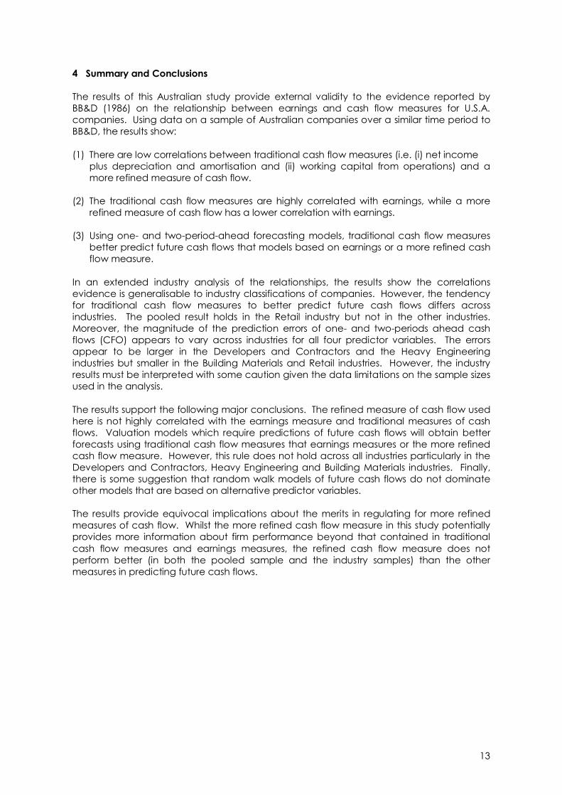
4 Summary and Conclusions

The results of this Australian study provide external validity to the evidence reported by BB&D (1986) on the relationship between earnings and cash flow measures for U.S.A. companies. Using data on a sample of Australian companies over a similar time period to BB&D, the results show:

(1) There are low correlations between traditional cash flow measures (i.e. (i) net income plus depreciation and amortisation and (ii) working capital from operations) and a more refined measure of cash flow.

(2) The traditional cash flow measures are highly correlated with earnings, while a more refined measure of cash flow has a lower correlation with earnings.

(3) Using one and twoperiodahead forecasting models, traditional cash flow measures better predict future cash flows that models based on earnings or a more refined cash flow measure.

In an extended industry analysis of the relationships, the results show the correlations evidence is generalisable to industry classifications of companies. However, the tendency for traditional cash flow measures to better predict future cash flows differs across industries. The pooled result holds in the Retail industry but not in the other industries. Moreover, the magnitude of the prediction errors of one and twoperiods ahead cash flows (CFO) appears to vary across industries for all four predictor variables. The errors appear to be larger in the Developers and Contractors and the Heavy Engineering industries but smaller in the Building Materials and Retail industries. However, the industry results must be interpreted with some caution given the data limitations on the sample sizes used in the analysis.

The results support the following major conclusions. The refined measure of cash flow used here is not highly correlated with the earnings measure and traditional measures of cash flows. Valuation models which require predictions of future cash flows will obtain better forecasts using traditional cash flow measures that earnings measures or the more refined cash flow measure. However, this rule does not hold across all industries particularly in the Developers and Contractors, Heavy Engineering and Building Materials industries. Finally, there is some suggestion that random walk models of future cash flows do not dominate other models that are based on alternative predictor variables.

The results provide equivocal implications about the merits in regulating for more refined measures of cash flow. Whilst the more refined cash flow measure in this study potentially provides more information about firm performance beyond that contained in traditional cash flow measures and earnings measures, the refined cash flow measure does not perform better (in both the pooled sample and the industry samples) than the other measures in predicting future cash flows.

14

Appendix – Predictions of Cash Flows: Within Industry

DEVELOPERS AND CONTRACTORS Medians (and Average Ranks)* of Absolute Forecast Errors

Scaled by the Actual Value of the Forecasted Series Predictor Variables

Dependent Variables NIBEI NIDPR WCFO CFO Panel A: One Period Ahead Forecasts

NIBEI** .228

()

NIDPR .345 .182

(2.00) (1.00)

WCFO .328 .197 .240

(3.00) (1.20) (1.80)

CFO .756 .736 .773 .992

(1.90) (2.70) (2.20) (3.20)


NIBEI** .324

()

NIDPR .439 .322

(2.00) (1.00)

WCFO .414 .294 .349

(2.78) (1.44) (1.78)

CFO .887 .853 .838 .985

(2.22) (2.67) (2.67) (2.44)

* Ranks based on the median forecast error across predictor variable in a given year are averaged across ten years in Panel A or nine years in Panel B

** A random walk model of NIBEI is presented as a benchmark

15

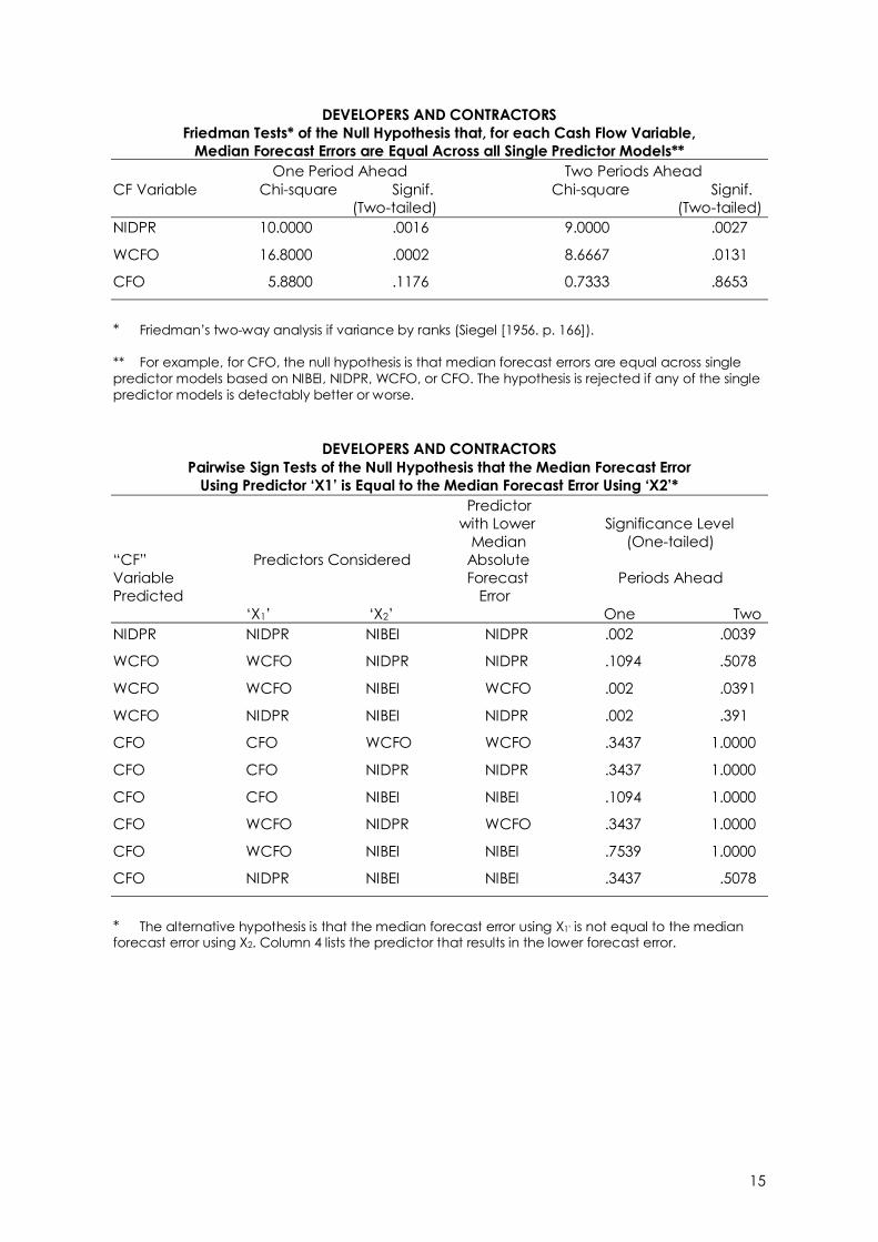
DEVELOPERS AND CONTRACTORS Friedman Tests* of the Null Hypothesis that, for each Cash Flow Variable,

Median Forecast Errors are Equal Across all Single Predictor Models** One Period Ahead Two Periods Ahead

CF Variable Chisquare Signif. Chisquare Signif. (Twotailed) (Twotailed)

NIDPR 10.0000 .0016 9.0000 .0027

WCFO 16.8000 .0002 8.6667 .0131

CFO 5.8800 .1176 0.7333 .8653

* Friedman’s twoway analysis if variance by ranks (Siegel [1956. p. 166]).

** For example, for CFO, the null hypothesis is that median forecast errors are equal across single predictor models based on NIBEI, NIDPR, WCFO, or CFO. The hypothesis is rejected if any of the single predictor models is detectably better or worse.

DEVELOPERS AND CONTRACTORS Pairwise Sign Tests of the Null Hypothesis that the Median Forecast Error

Using Predictor ‘X1’ is Equal to the Median Forecast Error Using ‘X2’* Predictor

with Lower Significance Level Median (Onetailed)

“CF” Predictors Considered Absolute Variable Forecast Periods Ahead Predicted Error

‘X1’ ‘X2’ One Two NIDPR NIDPR NIBEI NIDPR .002 .0039

WCFO WCFO NIDPR NIDPR .1094 .5078

WCFO WCFO NIBEI WCFO .002 .0391

WCFO NIDPR NIBEI NIDPR .002 .391

CFO CFO WCFO WCFO .3437 1.0000

CFO CFO NIDPR NIDPR .3437 1.0000

CFO CFO NIBEI NIBEI .1094 1.0000

CFO WCFO NIDPR WCFO .3437 1.0000

CFO WCFO NIBEI NIBEI .7539 1.0000

CFO NIDPR NIBEI NIBEI .3437 .5078

* The alternative hypothesis is that the median forecast error using X1' is not equal to the median forecast error using X2. Column 4 lists the predictor that results in the lower forecast error.

16

BUILDING MATERIALS Medians (and Average Ranks)* of Absolute Forecast Errors



NIBEI** .204

()

NIDPR .448 .174

(2.00) (1.00)

WCFO .422 .172 .176

(3.00) (1.40) (1.60)

CFO .451 .317 .304 .457

(2.90) (2.10) (1.90) (3.10)


NIBEI** .331

()

NIDPR .525 .260

(2.00) (1.00)

WCFO .497 .248 .267

(3.00) (1.56) (1.44)

CFO .517 .351 .346 .466

(3.33) (1.67) (2.11) (2.89)

* Ranks based on the median forecast error across predictor variables in a given year are averaged across ten years in Panel A or nine years in Panel B.

** A random walk model of NIBEI is presented as a benchmark.

17

BUILDING MATERIALS Friedman Tests* of the Null Hypothesis that, for each Cash Flow Variable,



NIDPR 10.0000 .0016 9.0000 .0027

WCFO 15.2000 .0005 13.5556 .0011

CFO 6.2400 .1005 9.1333 .0276



BUILDING MATERIALS Pairwise Sign Tests of the Null Hypothesis that the Median Forecast Error





WCFO WCFO NIDPR NIDPR .7539 1.0000



CFO CFO WCFO WCFO .1094 .5078

CFO CFO NIDPR NIDPR .1094 .1797

CFO CFO NIBEI 1.0000 1.0000

CFO WCFO NIDPR .7539 .5078

CFO WCFO NIBEI WCFO .3437 .0391

CFO NIDPR NIBEI NIDPR .3437 .0391


18

HEAVY ENGINEERING Medians (and Average Ranks)* of Absolute Forecast Errors



NIBEI** .283

()

NIDPR .401 .224

(1.90) (1.10)

WCFO .396 .209 .228

(2.80) (1.40) (1.80)

CFO .690 .862 .779 .996

(1.80) (2.60) (2.30) (3.30)


NIBEI** .430

()

NIDPR .491 .350

(1.89) (1.11)

WCFO .486 .325 .357

(2.78) (1.67) (1.56)

CFO .787 .769 .737 .894

(2.22) (2.89) (2.33) (2.56)



19

HEAVY ENGINEERING Friedman Tests* of the Null Hypothesis that, for each Cash Flow Variable,



NIDPR 6.4000 .0114 5.4444 .0196

WCFO 10.4000 .0055 8.2222 .0164

CFO 7.0800 .0694 1.4000 .7055



HEAVY ENGINEERING Pairwise Sign Tests of the Null Hypothesis that the Median Forecast Error





WCFO WCFO NIDPR NIDPR .3437 1.0000



CFO CFO WCFO WCFO .1094 1.0000

CFO CFO NIDPR NIDPR .3437 1.0000

CFO CFO NIBEI NIBEI .1094 1.0000

CFO WCFO NIDPR WCFO .7539 .5078

CFO WCFO NIBEI NIBEI .3437 1.0000

CFO NIDPR NIBEI NIDPR .3437 .5078


20

RETAIL Medians (and Average Ranks)* of Absolute Forecast Errors



NIBEI** .172

()

NIDPR .291 .163

(1.90) (1.10)

WCFO .253 .157 .150

(2.70) (1.70) (1.60)

CFO .552 .487 .500 .770

(2.00) (2.20) (2.20) (3.60)


NIBEI** .297

()

NIDPR .383 .267

(2.00) (1.00)

WCFO .340 .201 .257

(2.89) (1.00) (2.11)

CFO .536 .435 .449 .736

(2.67) (1.89) (1.78) (3.67)



21

RETAIL Friedman Tests* of the Null Hypothesis that, for each Cash Flow Variable,



NIDPR 6.4000 .0114 9.0000 .0027

WCFO 7.4000 .0247 16.2222 .0003

CFO 9.8400 .0200 12.3333 .0063



RETAIL Pairwise Sign Tests of the Null Hypothesis that the Median Forecast Error





WCFO WCFO NIDPR NIDPR 1.0000 .0039



CFO CFO WCFO WCFO .1094 .0391

CFO CFO NIDPR NIDPR .0215 .0391

CFO CFO NIBEI NIBEI .0215 .0391

CFO WCFO NIDPR WCFO .7539 1.0000

CFO WCFO NIBEI .7539 .0391

CFO NIDPR NIBEI NIDPR 1.0000 .5078


22

REFERENCES

Antle, R., Demski, J.S., and S.C. Ryan. [1989]. “Accounting Earnings with Multiple Sources of Information.” unpublished paper, Yale University.

Australian Stock Exchange. [1989]. Stock Exchange Indices and Statistics. Sydney.

Bernard, V.L., and R. G. Rulan, [1987]. “the Incremental Information content of Historical Cost and Current Cost Income Numbers: Time Series Analysis for 1962 to 1980”. The Accounting Review, October, pp. 707722.

Bernard, V.L., and T. Stober, [1989], “The Nature and Amount of Information in Cash Flows and Accruals”, The Accounting Review, October, pp. 624652.

Bowen, R.M., D. Burgstahler, and L.A. Daley, [1986]. “ Evidence on the Relationships Between Earnings and Various Measures of Cash Flow”, The Accounting Review, October, pp. 713725

Foster, G., [1986], Financial Statement Analysis, 2 nd Ed., PrenticeHall, New Jersey.

Lobo, G.J., and InMan Song, [1989], “The Incremental Information in SFAC No. 33 Income Disclosures over Historical Cost Income and its Cash and Accrual Components”, The Accounting Review, April, pp. 329343.

Siegel, S., [1956], NonParametric Statistics for the Behavioural Sciences, McGrawHill, New York.

Documents

Eprints Cover Sheeteprints.qut.edu.au/2028/1/2028_2.pdf · Tests of the three issues require that measures be obtained for ... Whilst it is arguable that abnormal items are transitory