arX

iv:c

ond-

mat

/051

0032

v1 [

cond

-mat

.sof

t] 3

Oct

200

5 Epitaxial Transition from Gyroid to Cylinder in a

Diblock Copolymer Melt

Takashi Honda ∗ Toshihiro Kawakatsu †

September 23, 2005

Abstract

An epitaxial transition from a bicontinious double gyroid to a hexagonally packed cylinderstructure induced by an external flow is simulated using real-space dynamical self-consistentfield technique. In order to simulate the structural change correctly, we introduce a systemsize optimization technique by which emergence of artificial intermediate structures are sup-pressed. When a shear flow in [111] direction of the gyroid unit cell is imposed, a nucleationand growth of the cylinder domains is observed. We confirm that the generated cylindricaldomains grow epitaxially to the original gyroid domains as gyroid d{220} → cylinder d{10}.In a steady state under the shear flow, the gyroid shows different reconnection processesdepending on the direction of the velocity gradient of the shear flow. A kinetic pathway pre-viously predicted using the self-consistent field theory where three fold junctions transforminto five fold junctions as an intermediate state is not observed.KEYWORDS: diblock copolymer, bicontinuous double gyroid, self-consisten field theory,dynamical mean field theory, epitaxial transition

1 Introduction

In the past, the self-organized microdomain structures of diblock copolymers have been thetarget of extensive studies 1, 2, 3, 4. Especially, the order-order transitions (OOTs) betweenthe microdomain structures are one of the central issues of the current experimental andtheoretical studies. Among various microdomain structures, the bicontinuous double gyroid(G) structure has attracted a great interest because of its complex structure (space groupIa3d) 5. Although this G phase exists only in a narrow region of the phase diagram ofa diblock copolymer, i.e. the region between the lamellar (L) phase and the hexagonallypacked cylinder (C) phase 6, its complex domains are expected to have a wide applicabilityto various techniques, for example, microporous systems, nano-reactors, and so on 7, 8, 9.

Experimentally, the OOT from the G phase to the C phase is believed to be an epitaxialtransition where the created cylindrical domains are commensurate to the original gyroiddomains. However, the microscopic detailed process of this epitaxial transition has not beenunderstood yet.

∗Japan Chemical Innovation Institute, and Division of Polymer, Faculty of Engineering, Tokyo Institute

of Technology, Ookayama, Meguro-ku, Tokyo 152-8552, Japan†Department of Physics, Tohoku University, Aoba, Aramaki, Aoba-ku, Sendai 980-8578, Japan

Epitaxial relationships between the G and C structures were observed in several exper-iments. Upon a temperature change, Rancon and Charvolin have observed that the {10}plane of the C is in commensurate to the {211} plane of the G domains in a surfactantsystem 10. In the present paper, we will use simple notation as C {10} → G {211} for suchan epitaxial relationships between planes.

An external shear flow also accelerates the OOTs. Under a shear flow and a temperaturechange, Schulz et al. have found different epitaxial relationships C {10} → G {220} and C{11} → G {211} in a block copolymer mixture by small-angle neutron scattering (SANS)experiments 11. Under similar experimental conditions using small-angle X-ray scattering(SAXS) diffraction techniques, Forster et al. have observed the epitaxial relationship C{10} → G {211} similar to the Rancon and Charvolin’s observation 12. The same epitaxialrelationship was also observed by Vigild et al. in a block copolymer system using SANS 13.A cyclic transition C → G → C in a block copolymer solution has been studied by Wangand Lodge, who supported the epitaxial relationship G {211} → C {10} 15.

From the point of view of kinetics, a long-lived coexistence between the C phase and theG phase has been found in the C → G of a block copolymer system under a shear flow anda temperature change 14. Furthermore, a grain boundary between the C phase and the Gphase has been observed by a polarized optical microscopy in a quenched polymer solution16. These observations suggest an existence of a stable boundary between the C phase andthe G phase.

On the theoretical side, mean field theories have been used to investigate microdomainstructures of diblock copolymers. Using the self-consistent field (SCF) technique, Helfandand Wasserman have evaluated the free energy and predicted the equilibrium domain sizes ofthe classical phases in the strong segregation regime such as the body centered cubic crystalof spherical domains (BCC), the C phase, and the lamellar (L) phase 17, 18, 19. On the otherhand, the phase diagram of diblock copolymer in the weak segregation regime was predictedby Leibler using the random phase approximation (RPA) 20. Leibler’s phase diagram is com-posed of classical phases and the disordered (D) phase depending on the values of the blockratio and the χN , i.e. the product of the Flory-Huggins interaction parameter χ and thetotal degree of polymerization of diblock copolymer N . The entire phase diagram includingboth the weak segregation regime and the strong segregation regime has been constructed byMatsen and Shick using the SCF technique in the reciprocal lattice space. Besides the clas-sical phases, they predicted the complex G phase in the weak and intermediate segregationregime 1, 21. This theoretical phase diagram was confirmed experimentally 22.

Despite the success of the mean field theories on the equilibrium phase behavior, theinvestigation on the dynamic properties has not been fully developed yet. There have beena few trials on the dynamics of OOTs and order-disorder transitions (ODTs) of the mi-crodomain structures of diblock copolymers using the mean field approximation. A timedependent Ginzburg-Landau (TDGL) model was used to investigate the instability in theOOTs and ODTs such as OOTs L → C and L → S, and C → S. 23, 24, 25. In these studies,the authors retained the most unstable modes in the Fourier amplitudes of the density fluc-tuations emerging in the vicinity of the critical point. A TDGL model described in termsof Fourier modes with two sets of wave vectors with different magnitudes has been used tostudy the transitions D → G, G → C, and so on 26, 27, 28. Although the TDGL theory isefficient in investigating large-scale systems, it is in principle applicable only to the weaksegregation regime.

On the other hand, the SCF theory can be used to study the phase transitions in weak,

intermediate and strong segregation regimes. The quantitative accuracy of the SCF theory isanother advantage compared to the TDGL theory. This is because the SCF theory takes theconformational entropy of the polymer chains into account precisely 17, 29, 30, 31. Using theSCF theory, Laradji et al. have investigated the epitaxial transitions such as L ↔ C, C ↔ S,and G → C taking the anisotropic fluctuations into account 32, 33. Matsen has also studiedthe transitions C ↔ S and C ↔ G using the SCF theory and has proposed a nucleation andgrowth model of the epitaxial transitions 34, 35.

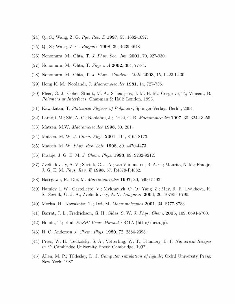
All of these theoretical studies mentioned above rely on the reciprocal space representa-tions 28, 32, 35 and most of experimental studies 10, 12, 13 have supported the existence of theepitaxial OOT G {211} ↔ C {10} except for Schulz et al., who have supported the epitaxialOOT G {220} ↔ C {10}. Experimentally, the epitaxial OOT G {211} ↔ C {10} and G{220} ↔ C {10} are recognized as the same epitaxial relationships 13 because the diffractionpeaks from both G {211} and G {220} match well with the diffraction peaks from the C{10}. In this argument, however, the kinetic pathway in real space was not considered. InFigure 1, we show a projection of the G structure onto the [111] direction in the real space.The epitaxial relations G {211} ↔ C {10} and G {220} ↔ C {10} are shown in Figure1(a) and 1(b), respectively, where the spacing of the G planes and the epitaxial cylindricaldomains are shown. As the directions of these two planes G {112} and G {220} are perpen-dicular with each other and the spacings between adjacent planes are also different, the twogrowth mechanisms shown in Figures 1(a) and (b) should be regarded as different ones.

Furthermore, the OOTs of block copolymer melts are first order phase transitions andthe nucleation and growth process of domains is expected. Since these process is spatiallyinhomogeneous, such a transition is not compatible with the treatment in the reciprocal lat-tice space (Fourier space), where spatially periodic lattice structures are assumed. Therefore,dynamical simulations in real space, such as the dynamical SCF simulation, is necessary tocorrectly investigate this transition 36, 37, 38, 39.

In the present paper, we study the epitaxial OOT G → C using the dynamical SCFtheory under shear flows. In order to treat the first order transition, we introduce a systemsize optimization (SSO) method, in which the side lengths of the simulation box are auto-matically adjusted so that the size and the shape of the simulation box are fit for the latticespacing and the lattice axes of the ordered structures. Recently, Barrat et al. proposed asimilar technique to study equilibrium domain morphology of block copolymer systems 41.In the course of the transition, we observe a complex transient state that is composed ofcylindrical domains parallel to the G {220} plane. We also confirm that our SSO methodcan reproduce spatially inhomogeneous nucleation and growth processes. Actually we ob-serve the coexistence between the G phase and the C phase, which is consistent with theexperimentally observed first order transition behavior 16. Furthermore we found that the Gstructure shows different deformation behaviours depending on the direction of the velocitygradient of the shear flow.

We cannot confirm the scenario of the transition proposed by Matsen 35, where the threefold junctions transform into five fold junctions.

Finally, we clarify the kinetic pathway from the G phase to the C phase under a shearflow. To the best of our knowledge, this kinetic pathway in the real space has not beenreported in the literature.

2 Theory

2.1 Dynamical self-consistent field theory

Here, we briefly summarize the SCF theory for an A-B diblock copolymer 4, 30, 36, 40. Letus consider a melt of A-B diblock copolymer. Due to the screening effect in the melts, wecan assume Gaussian statistics for the chain conformation. Within this Gaussian statistics,the K-type (K =A or B) segment is characterized by the effective bond length bK , and theK-type block is characterized by the degree of polymerization NK . Then the total degreeof polymerization N is defined as N ≡ NA + NB. We introduce an index s to specify eachsegment, where s = 0 corresponds to the free end of the A-block and s = N corresponds tothe other free end of the B-block. Therefore, 0 ≤ s ≤ NA and NA ≤ s ≤ N correspond to theA- block and the B-block, respectively. In order to evaluate the conformational entropy, weneed the statistical weight of any subchains. Let us use the notation Q(s′, r′; s, r) to denotethe statistical weight of a subchain between s-th and s′-th segments (0 ≤ s′ ≤ s ≤ N) thatare fixed at the positions r and r′. This statistical weight can be obtained by solving thefollowing Edwards equation within the mean-field approximation

∂

∂sQ(s′, r′; s, r) =

[b(s)2

6∇2 − βV (s, r)

]Q(s′, r′; s, r), (1)

where β = 1/(kBT ), b(s) = bK if the s-th segment is the K-type segment, and V (s, r) is anexternal potential acting on the s-th segment at r imposed by the surrounding segments.Here, we assume that the external potential V (s, r) is the same if the segment species (A orB) is the same. Thus,

V (s, r) =

{VA(r) if s indicates an A-segmentVB(r) if s indicates a B-segment.

(2)

Equation (1) should be supplemented by the initial condition Q(0, r′; 0, r) = δ(r′−r). As thetwo ends of the block copolymer are not equivalent, we should introduce another statisticalweight Q(s′, r′; s, r), which is calculated in the opposite direction along the chain startingfrom the free end s = N .

To reduce the computational cost, we define an integrated statistical weights q(s, r) andq(s, r)as follows:

q(s, r) ≡∫

dr′Q(0, r′; s, r)

q(s, r) ≡∫

dr′Q(0, r′; s, r). (3)

It is easy to confirm that q(s, r) and q(s, r) also satisfy eq. (1).By using eqs. (3), the density of the K-type segments at position r is given by

φK(r) = C∫

s∈K−blockds q(s, r)q(N − s, r), (4)

where C is the normalization constant:

C =M

∫dr

∫dsq(s, r)q(N − s, r)

=M

Z . (5)

The parameter M is the total number of chains in the system and Z is the single chainpartition function which is independent of K, i.e. Z =

∫drq(s, r)q(N −s, r) =

∫drq(N, r) =∫

drq(N, r) .The external potential VK(r) can be decomposed into two terms as follows

VK(r) =∑

K ′

ǫKK ′φK ′(r) − µK(r). (6)

The first term is the interaction energy between segments and the ǫKK ′ is the nearest-neighbor pair interaction energy between a K-type segment and a K ′-type segment, whichis related to the Flory-Huggins interaction parameter via χAB ≡ zβ[ǫAB − (1/2)(ǫAA + ǫBB)]where z is the number of nearest neighbor sites. The µK(r) is the chemical potential ofthe K-type segment, which is the Lagrange multiplier that fixes the density of the K-typesegments at the position r to the specified density value. The VK(r) must be determined ina self-consistent manner so that this constraint is satisfied. Such a self-consistent conditionis achieved by an iterative refinement of the VK(r).

To improve the stability of the numerical scheme, we used the following finite differencescheme for the Edwards equation, eq. (1)

q(s + ∆s, r) = exp[−βV (s, r)∆s

2](1 +

b(s)2

6∇2∆s

)exp[−βV (s, r)∆s

2]q(s, r). (7)

The Helmholtz free energy of the system can be given as follows

F = −kBTM lnZ +1

2

∑

K

∑

K ′

∫drǫKK ′φK(r)φK ′(r) −

∑

K

∫drVK(r)φK(r). (8)

To introduce dynamics into the model, we assume Fick’s law of linear diffusion for thesegment densities and an effect of the flow advection as follows

∂

∂tφK(r, t) = LK∇2µK(r) −∇{v(r, t)φK(r, t)}, (9)

where LK is the mobility of K-type segment and v(r, t) is the local flow velocity such as thevelocity of the externally imposed shear flow.

2.2 System size optimization method

Periodic microdomain structures of diblock copolymers have the crystal symmetry. To ob-tain equilibrium states of these periodic structures using the mean field theory, the freeenergy density of the system must be minimized with respect to the lattice structures ofthe ordered microdomains. Same is true for two phase coexisting states where the systemsize should be optimized with respect to the coexisting two periodic structures. For thesepurpose we introduce the system size optimization (SSO) method that minimizes the freeenergy density of the system by optimizing the side lengths of the simulation box on whichperiodic boundary conditions are imposed. This is a similar method as the constant pressuremolecular dynamics simulation proposed by Andersen43. In the static SCF calculations, thisoptimization can be performed by requiring the following local equilibrium condition for eachside length of the simulation box:

∂F∂Li

= 0, (10)

where Li(i = x, y, z) is the side length of the simulation box. The left-hand side of eq. (10)can be evaluated numerically using the following central difference approximation

∂F∂Li

=F (Li + ∆Li) − F (Li − ∆Li)

2∆Li

, (11)

where ∆Li is a small variation of Li. We used the parabolic optimization method44 to solveeq. (10).

On the other hand, when the dynamical SCF calculation is performed, we should regardLi as a dynamical variable whose dynamics is described by the following ficticious equationof motion

∂Li

∂t= −ζi

∂F∂Li

, (12)

where ζi is a positive coefficient whose value is chosen properly so that the local equilibriumcondition eq.(10) for Li is guaranteed at every time step.

We checked the validity of our dynamical SSO method by using an A-B diblock copoly-mer melt whose stable equilibrium phase is the C phase. We performed two dimensionalsimulations where we assumed that ζx = ζy = ζ for simplicity, and we changed ζ from 0.0to 0.5. The parameters characterizing the A-B diblock copolymer are as follows: the totallength of the copolymer N = 20, the block ratio of the A block f = NA/N = 0.35, and theeffective bond lengths of each segment type are unity. The interaction parameter is set tobe χN = 15, which corresponds to the C phase in its equilibrium state 21. The initial stateis set to the D phase to which we added small random noise with the standard deviation0.0006. The initial shape of the simulation box is a square with side length 32.0. As thesquare shape of the simulation box is not compatible with the perfect C phase, the SSOmethod adjusts the side lengths of the simulation box automatically.

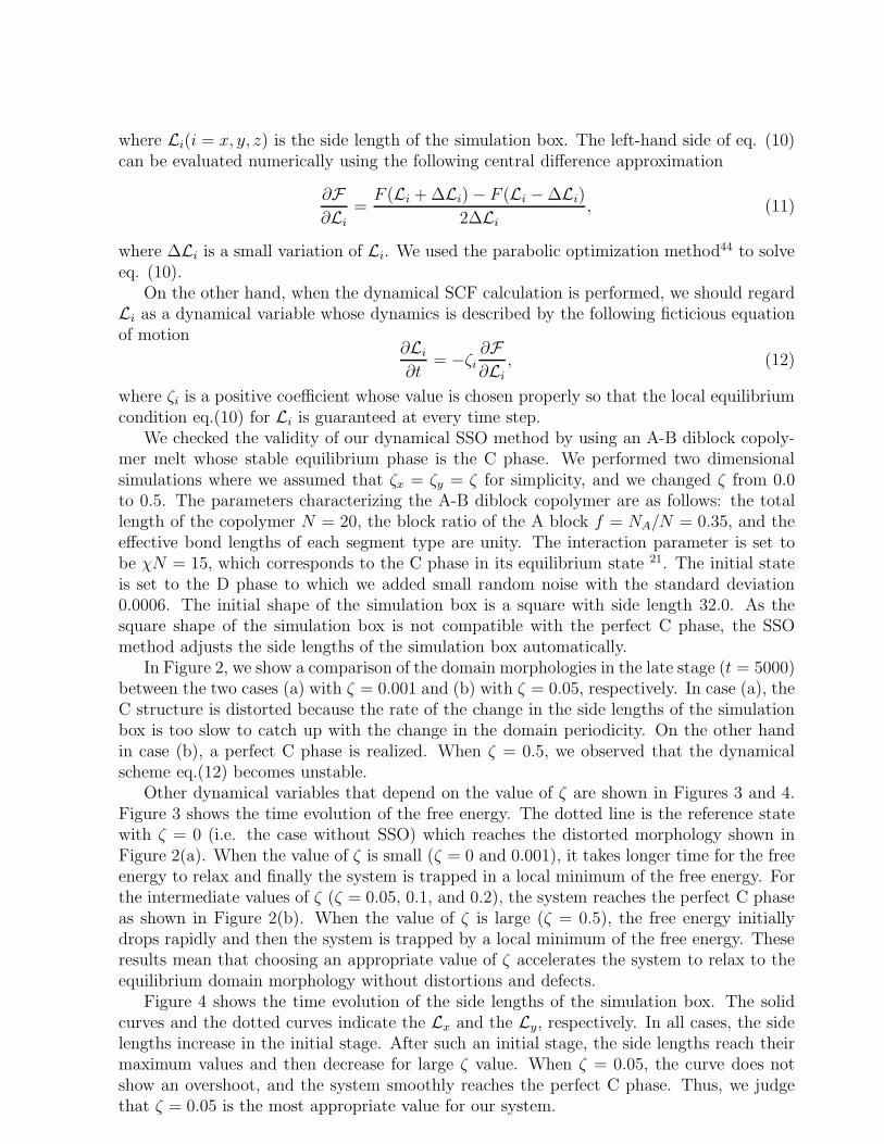
In Figure 2, we show a comparison of the domain morphologies in the late stage (t = 5000)between the two cases (a) with ζ = 0.001 and (b) with ζ = 0.05, respectively. In case (a), theC structure is distorted because the rate of the change in the side lengths of the simulationbox is too slow to catch up with the change in the domain periodicity. On the other handin case (b), a perfect C phase is realized. When ζ = 0.5, we observed that the dynamicalscheme eq.(12) becomes unstable.

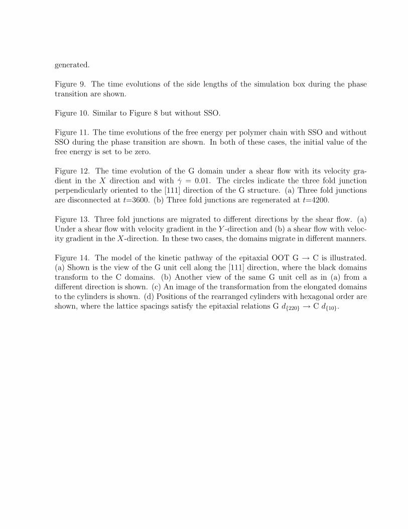
Other dynamical variables that depend on the value of ζ are shown in Figures 3 and 4.Figure 3 shows the time evolution of the free energy. The dotted line is the reference statewith ζ = 0 (i.e. the case without SSO) which reaches the distorted morphology shown inFigure 2(a). When the value of ζ is small (ζ = 0 and 0.001), it takes longer time for the freeenergy to relax and finally the system is trapped in a local minimum of the free energy. Forthe intermediate values of ζ (ζ = 0.05, 0.1, and 0.2), the system reaches the perfect C phaseas shown in Figure 2(b). When the value of ζ is large (ζ = 0.5), the free energy initiallydrops rapidly and then the system is trapped by a local minimum of the free energy. Theseresults mean that choosing an appropriate value of ζ accelerates the system to relax to theequilibrium domain morphology without distortions and defects.

Figure 4 shows the time evolution of the side lengths of the simulation box. The solidcurves and the dotted curves indicate the Lx and the Ly, respectively. In all cases, the sidelengths increase in the initial stage. After such an initial stage, the side lengths reach theirmaximum values and then decrease for large ζ value. When ζ = 0.05, the curve does notshow an overshoot, and the system smoothly reaches the perfect C phase. Thus, we judgethat ζ = 0.05 is the most appropriate value for our system.

The above-mentioned dynamical SCF simulation can be performed with use of the ”Sim-ulation Utilities for Soft and Hard Interfaces (SUSHI)” in OCTA system 42. The simulationresults reported in this article is obtained using SUSHI.

3 Simulation Results

We simulated the epitaxial OOT G → C by imposing an external shear flow to an A-Bdiblock copolymer that is characterized by the parameters given in Section 2.2 using thetechnique described in the previous section. The details of the simulation procedure aregiven below.

3.1 Initial gyroid structure and final cylindrical structure

The initial state of the simulation is chosen as the equilibrium G structure at χN = 20. Togenerate such an equilibrium G structure, we used the following procedure. Let us denotethe equilibrium (or steady state) side length of the unit cell of the G structure as DG, andthe equilibrium (steady state) spacing of the lamellar structure formed by the same blockcopolymer at χN = 20 as DL. The value of DL can easily be obtained using a one dimensionalSCF calculation with SSO. Then, assuming an epitaxial relationship in the transitions L{10}→ C {10} → G {211} at a fixed value of χN , we can obtain an approximant for DG as follows

DG =√

6DL. (13)

Using this value of DG as the initial size of the simulation box, we set the SCF potentialwith the G symmetry as

V (x, y, z) = V0

(cos

2πx

DG

sin2πy

DG

+ cos2πy

DG

sin2πz

DG

+ cos2πz

DG

sin2πx

DG

)2, (14)

where x, y, and z are the Cartesian coordinates, and the V0 is an arbitrary small coefficientwhich we assume to be 0.001 for the minor segments and -0.001 for the major segments.The use of the squared form on the right-hand side of eq.(14) originates from the fact thatthe gyroid structure in block copolymer melt is formed by double networks each with the Gsymmetry. By assigning different signs to the V0’s for major and minor segments, we can letthe minor phase to gather inside the gyroid network while the major phase becomes rich inthe matrix region.

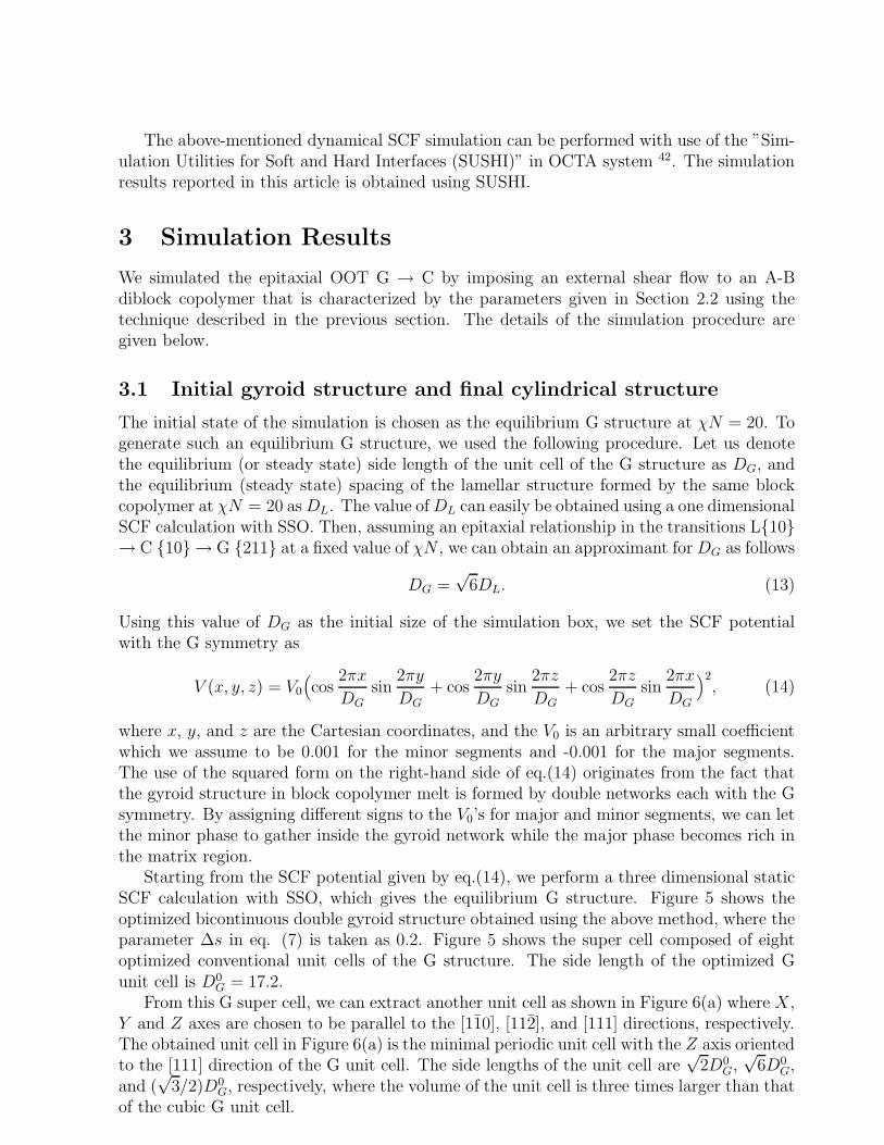
Starting from the SCF potential given by eq.(14), we perform a three dimensional staticSCF calculation with SSO, which gives the equilibrium G structure. Figure 5 shows theoptimized bicontinuous double gyroid structure obtained using the above method, where theparameter ∆s in eq. (7) is taken as 0.2. Figure 5 shows the super cell composed of eightoptimized conventional unit cells of the G structure. The side length of the optimized Gunit cell is D0

G = 17.2.From this G super cell, we can extract another unit cell as shown in Figure 6(a) where X,

Y and Z axes are chosen to be parallel to the [110], [112], and [111] directions, respectively.The obtained unit cell in Figure 6(a) is the minimal periodic unit cell with the Z axis orientedto the [111] direction of the G unit cell. The side lengths of the unit cell are

√2D0

G,√

6D0G,

and (√

3/2)D0G, respectively, where the volume of the unit cell is three times larger than that

of the cubic G unit cell.

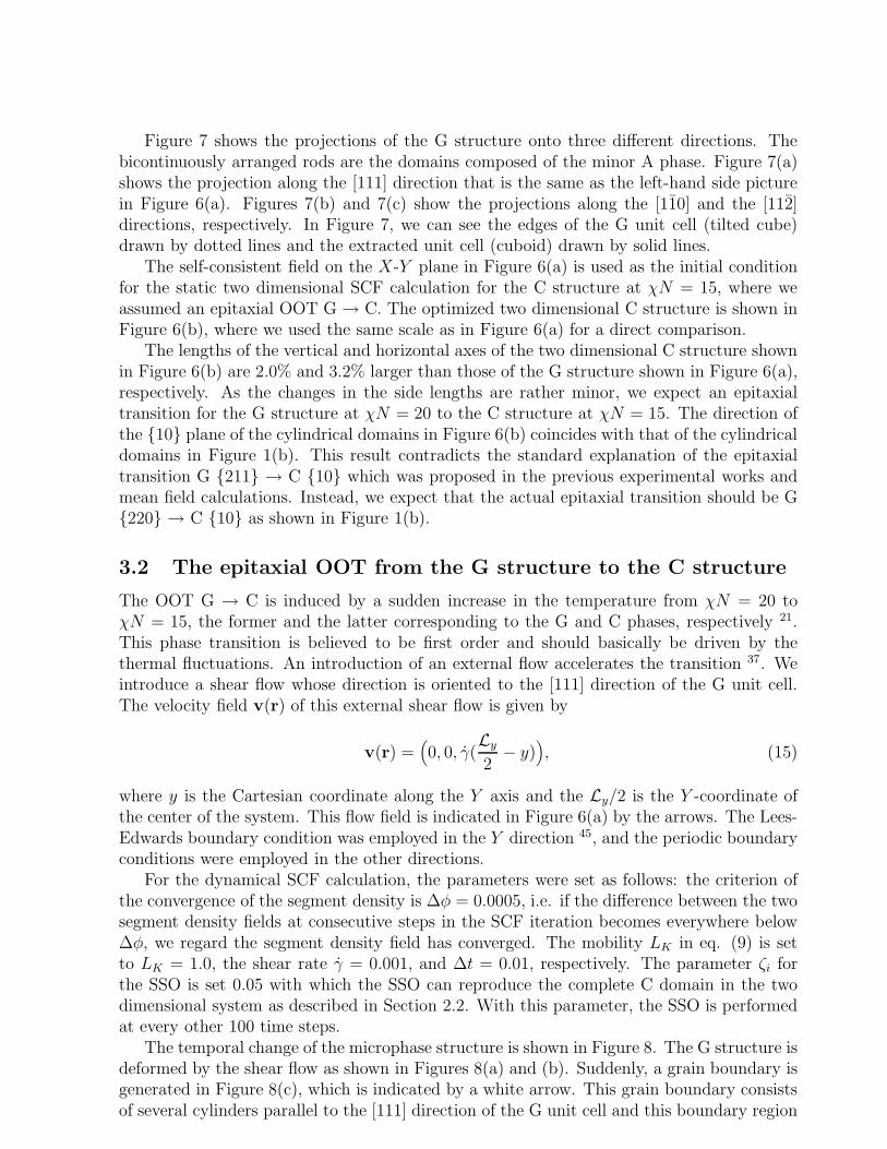
Figure 7 shows the projections of the G structure onto three different directions. Thebicontinuously arranged rods are the domains composed of the minor A phase. Figure 7(a)shows the projection along the [111] direction that is the same as the left-hand side picturein Figure 6(a). Figures 7(b) and 7(c) show the projections along the [110] and the [112]directions, respectively. In Figure 7, we can see the edges of the G unit cell (tilted cube)drawn by dotted lines and the extracted unit cell (cuboid) drawn by solid lines.

The self-consistent field on the X-Y plane in Figure 6(a) is used as the initial conditionfor the static two dimensional SCF calculation for the C structure at χN = 15, where weassumed an epitaxial OOT G → C. The optimized two dimensional C structure is shown inFigure 6(b), where we used the same scale as in Figure 6(a) for a direct comparison.

The lengths of the vertical and horizontal axes of the two dimensional C structure shownin Figure 6(b) are 2.0% and 3.2% larger than those of the G structure shown in Figure 6(a),respectively. As the changes in the side lengths are rather minor, we expect an epitaxialtransition for the G structure at χN = 20 to the C structure at χN = 15. The direction ofthe {10} plane of the cylindrical domains in Figure 6(b) coincides with that of the cylindricaldomains in Figure 1(b). This result contradicts the standard explanation of the epitaxialtransition G {211} → C {10} which was proposed in the previous experimental works andmean field calculations. Instead, we expect that the actual epitaxial transition should be G{220} → C {10} as shown in Figure 1(b).

3.2 The epitaxial OOT from the G structure to the C structure

The OOT G → C is induced by a sudden increase in the temperature from χN = 20 toχN = 15, the former and the latter corresponding to the G and C phases, respectively 21.This phase transition is believed to be first order and should basically be driven by thethermal fluctuations. An introduction of an external flow accelerates the transition 37. Weintroduce a shear flow whose direction is oriented to the [111] direction of the G unit cell.The velocity field v(r) of this external shear flow is given by

v(r) =(0, 0, γ(

Ly

2− y)

), (15)

where y is the Cartesian coordinate along the Y axis and the Ly/2 is the Y -coordinate ofthe center of the system. This flow field is indicated in Figure 6(a) by the arrows. The Lees-Edwards boundary condition was employed in the Y direction 45, and the periodic boundaryconditions were employed in the other directions.

For the dynamical SCF calculation, the parameters were set as follows: the criterion ofthe convergence of the segment density is ∆φ = 0.0005, i.e. if the difference between the twosegment density fields at consecutive steps in the SCF iteration becomes everywhere below∆φ, we regard the segment density field has converged. The mobility LK in eq. (9) is setto LK = 1.0, the shear rate γ = 0.001, and ∆t = 0.01, respectively. The parameter ζi forthe SSO is set 0.05 with which the SSO can reproduce the complete C domain in the twodimensional system as described in Section 2.2. With this parameter, the SSO is performedat every other 100 time steps.

The temporal change of the microphase structure is shown in Figure 8. The G structure isdeformed by the shear flow as shown in Figures 8(a) and (b). Suddenly, a grain boundary isgenerated in Figure 8(c), which is indicated by a white arrow. This grain boundary consistsof several cylinders parallel to the [111] direction of the G unit cell and this boundary region

separates the upper G phase and the lower G phase. The transition from the G structure tothe C structure takes place in this lower phase as shown in Figures 8(d)-(f). The cylindersare tilted to the [111] direction of the G unit cell as shown in the side view of Figure 8(f).

The tilting of the cylinders is caused by the constant shear flow because a steady shearflow is composed of two contributions, a uniaxial extension and a rotation 31. This rota-tional contribution tilts the cylinders. Such a tilting is suppressed in experiments by usingoscillatory shear flows.

Three fold junctions in the upper G phase shown in Figure 8 (f) are stable and aremigrated by the shear flow. Even in the late stage (t=10000), we cannot obtain the finalequilibrium C structure. This result suggests that boundary between the upper G phase andthe lower C phase is stable and the separated G and C phases coexist stably. Actually, aclear boundary between the G and C grains is observed by a polarized optical microscopyin a polymer solution 16 and the long-lived coexistence between the G and the C phases isexperimentally observed in a block copolymer 14.

The changes in the side lengths of the simulation box are shown in Figure 9. The sidelengths in the X and Z directions are almost constant, which means that the epitaxialcondition is satisfied. On the other hand, the side length in the Y direction increases withtime. The reason of the increase is explained below.

To check the effect of the SSO method, we carried out the same dynamical SCF simula-tion but without the SSO method. The time evolution of the domain morphology is shownin Figure 10. In this case, as shown in Figures 10(a)-(d), the OOT occurs at the center of thesystem where the G structure transforms into the C structure. The stable grain boundaryas shown in Figure 8 is, however, not observed in this case without SSO. The cylindricaldomains are also tilted to the [111] direction of the G unit cell as is shown in the side viewof Figure 10(c). After such a transient state, the system reaches the complete C structure.A characteristic phenomenon is observed near the center of the system where the cylindricaldomains reconnect as shown in Figures 8(d)-(f). Such reconnections continue steadily forcertain time duration. This reconnection phenomenon means that the system is in a dynam-ical steady state where the energy injected by the shear flow into the system is released bythe energy dissipation accompanied by the periodic reconnections of the cylindrical domains.

In order to check the stability of the systems, we show in Figure 11 the time evolution ofthe free energy density during the phase transition. The free energy density in the case withthe SSO shows a moderate change compared to that in the case without the SSO, whichshows an oscillation synchronized to the reconnections of the cylindrical domains. Such aperiodic change in the free energy density is observed after t = 3000 when the system reachesthe almost perfect C structure without defects. In order to obtain such a perfect C phase, thesystem goes over energy barriers by the driving force of the shear flow. In the case withoutSSO, however, the energy barrier should be much higher than the case with SSO becausethe condition of the constant system size imposes a sever restrictions on the reconnection ofthe cylindrical domains. In the case with SSO, such a restriction is avoided by the increasein the side length of the simulation box in the Y direction as shown in Figure 9.

We also tried simulations under a shear flow whose velocity gradient is set parallel to theX direction. In this case, the free energy of the system increases slightly but the nucleationand growth of cylindrical domains can not be observed even in the late stage t=6000 eitherwith SSO or without SSO. The epitaxial condition for the OOT is expected to be more pre-cise for this direction of the velocity gradient than the case with the velocity gradient in theY -direction. This is because the periodicity of the G structure in X direction matches the

periodicity of the C structure than that in the Y direction, the former promoting the gener-ation of the C structure. Contrary to this expectation, three fold junctions perpendicularlyoriented to the [111] direction of the G unit cell continue to disconnect and reconnect due tothe shear flow. Figure 12 shows this phenomenon. The circles in the Figure 12 indicate thethree fold junctions where the disconnections and the reconnections take place. Figure 12(a)shows the structure after the disconnections, where we can observe the remains of three foldjunctions indicated by the circles. Figure 12(b) shows the structure after the reconnections,where the three fold junctions regenerated. This result indicates that the G structure hasdifferent stabilities to different directions of the shear velocity gradient.

The reason of this different stability is explained by using Figure 13. Figure 13 showsthree fold junctions perpendicularly oriented to the [111] direction of the G unit cell withdifferent rotational angles to the direction of the shear gradient. Figure 13(a) shows a threefold junction under a shear flow with its velocity gradient in the Y direction. The threedomains extending from the center of the three fold junction are subjected to different shearflow velocities, i.e. the three domains do not move with the same velocity vy. Thus, thethree domains are elongated to the different directions with different rates, and the elongationfinally makes the three fold junction disconnected. On the other hand, in the case of a threefold junction under a shear flow with its velocity gradient in the X direction as shownin Figure 13(b), two domains have the same velocity vx. In this situation, the three foldjunction is elongated to the positive direction of the X-axis. Even after the disconnection,the separated domains keep closer and will be reconnected easily to form the three foldjunction structure as shown in Figure 12.

4 Discussions

Our simulation showed that the epitaxial OOT G → C takes place in the [111] directionof the G unit cell and that the epitaxial relation for the G {220} → C {10} transition isachieved. The transition does not occur uniformly as shown in Figures 8(d)-(f) and Figure10(c), where the C domain nucleates and grows.

Most of the experiments have reported the epitaxial OOT C {10} ↔ G {211} whichdisagrees with our simulation result. A possible reason of this discrepancy is as follows. Thefirst diffraction peak from a G structure is the peak from {211} and the intensity of thispeak is stronger than that of {220} peak (secondary peak). Moreover, the positions of thepeaks from G {220}, G {211} and C {10} are so close that it is not easy to judge which ofthe peaks from G {220} and G {211} epitaxially matches with the peak from C {10}. Wecalculated a three dimensional scattering function of the optimized G structure obtained inthe simulation, and confirmed that the {211} spots are dominant and their intensities areabout four times larger than those of the {220} spots.

If the G {211} → C {10} is realized under a shear flow with the velocity gradient in theY direction, the planes composed of cylinders are directed in parallel to the sheared plane,i.e. the XZ plane. Thus, the friction generated by the reconnecting domains to the shearflow is expected to be smaller than that for the G {220} → C {10} case where the cylinderplanes are perpendicular to the sheared plane. In our simulations, however, the systemprefers the pathway as G {220} → C {10}. Therefore, we conclude that the direction ofthe velocity gradient is not an important factor in determining the direction of the C planesfor the epitaxial transition. On the other hand, we confirmed that matching between the

lattice constants is more important. As is shown in Figure 6(b), the origin of the selectionof the generated C structure from the G [111] plane (Figure 6(a)) is the matching betweenthe lattice constants. That is, the system prefers the kinetic pathway that minimizes thefree energy of the system by matching the lattice constants, which leads to the G {220} →C {10} transition.

Previous theoretical studies have also supported the OOT G {211} → C {10}. Thesestudies relied on the reciprocal space representations. However most of the experiments havebeen done under a condition with a shear flow and a temperature change. We succeeded inreproducing such experimental conditions in our simulation. Using this simulation, we couldreproduce the correct kinetic pathway of the epitaxial OOT, i.e. the nucleation and growthprocess of the C domains.

We found the difference in the stability of the G domains to the shear gradient directiondue to the different velocities of the shear flow imposed on the three domains meeting at athree fold junction as shown in Figures 12 and 13. The G structure is stable under the shearflow with the velocity gradient in the X direction. There has been no answer to the questionwhy the complex G phase with three dimensional bicontinuous structure is generated undera shear flow. Our result demonstrates that the G structure is actually stable under a shearflow.

Although the detail of the transition process is complex, we understand that the threefold junctions with domains perpendicular to the [111] direction of the G unit cell do notplay an important role in the transformation from G to C. Three fold junctions are simplydisconnected and vanish during the phase transition. This observation does not agree withthe model of the epitaxial transition proposed by Matsen, where a three fold junction isconnected to one of the nearest neighbor three fold junctions to form a five fold junction.In our observation, three fold junctions are stable and they are not connected to any otherjunctions.

Here, we propose a model of the kinetic pathway. Figure 14(a) shows a projection of the Gunit cell along the [111] direction, where the bold triangles are the projections of consecutivethree domains. Figure 14(b) is the same structure as Figure 14(a) observed from a differentdirection. We can confirm that the triangles in Figure 14(a) are formed by consecutive threedomains (shown in black) connected by three fold junctions. When a shear flow is imposed,these black domains in Figure 14(b) are elongated and form cylinders as shown in Figure14(c). These cylinders are rearranged to form a hexagonally packed cylindrical structurewhose lattice spacings satisfy the epitaxial relations G {220} → C {10} as shown in Figure14(d). This model of the kinetic pathway can be verified in Figures 8(d)-(e) and in Figures10(b)-(c).

5 Conclusion

The epitaxial OOT G → C was studied using the real space dynamical SCF technique withthe SSO method. With such an SSO method, we succeeded in reproducing the realistickinetic pathway of the first order phase transition of G → C. On the other hand, in theabsence of the SSO, we found that the kinetic pathway is very different from what weobserve with SSO. We also found that the G structure shows different responses to differentdirections of the velocity gradient of the shear flow.

Using this technique, we studied the kinetic pathway of the G → C transition induced

by a shear flow in the [111] direction of the unit cell of the G structure. We observed thefollowing kinetic pathway: The G domains perpendicularly oriented to the [111] directionof the G unit cell do not contribute to the formation of the cylindrical domains. They aredisconnected and vanish during the transition. On the other hand, the other G domains areelongated by the shear flow and transform into the cylindrical domains. Such deformationsoccur locally, and the cylindrical domains are rearranged to form a hexagonally close-packedC structure.

The most important result of our simulations with SSO is that we can observe a nucleationand growth of the C phase in the matrix of the G phase, i.e. the nature of the first orderphase transition, which was not observed in the previous simulations done in the Fourierspace. Under a steady shear flow, we observed that the G domains around the nucleus of theC phase deform and gradually join the C phase. We also observed that the domain spacingsatisfies the epitaxial relationship G {220} → C {10} as was proposed in the experimentalwork 11. We could not observe the transformation process of the domains from three foldjunctions to five fold junctions as was previously proposed 35.

We found that the dynamical SCF theory with the SSO method in real space is veryuseful and reliable to trace the OOTs and ODTs between the microdomain structures ofblock copolymer melts.

Acknowledgment

T. H. thanks Dr. H. Kodama and Dr. R. Hasegawa for the fruitful collaborations incoding SUSHI. The authors thank Prof. M. Doi (Tokyo University) and the members of theOCTA project for many helpful comments and discussions. This study is executed underthe national project, which has been entrusted to the Japan Chemical Innovation Instituteby the New Energy and Industrial Technology Development Organization (NEDO) underMETI’s Program for the Scientific Technology Development for Industries that Creates NewIndustries. This work is partially supported by Grant-in-Aid for Science from the Ministryof Education, Culture, Sports, Science and Technology, Japan. The computation was in partperformed at the Super Computer Center of the Institute of Solid State Physics, Universityof Tokyo.

References

(1) Matsen, M. W.; Bates, F. S. Macromolecules 1996, 29, 1091-1098.

(2) Hamley, I. W. Block Copolymers ; Oxford University Press: Oxford, 1999.

(3) Bates, F. S.; Fredrickson, G. H. Physics Today 1999, 52, 32-38.

(4) Fredrickson, G. H.; Ganesan, V.; Drollet, F. Macromolecules 2002, 35, 16-39.

(5) Hajduk, D. A.; Harper, P. E.; Gruner, S. M.; Honeker, C. C.; Kim, G.; Thomas, E. L.;Fetters, L. J. Macromolecules 1994, 27, 4063-4075.

(6) Matsen, M. W.; Bates, F. S. J. Chem. Phys 1997, 106, 2436-2448.

(7) Hashimoto, T.; Tsutsumi, K.; Funaki, Y. Langmuir 1997, 13, 6869-6872.

(8) Zhao, D.; Feng, J.; Huo, Q.; Melosh, N.; Fredrickson, G. H.; Chmelka, B. F.; Stucky,G. D. Science 1998, 279, 548-552.

(9) Chan, V. Z.-H.; Hoffman, J.; Lee, V. Y.; Iatrou, H.; Avgeropoulos, A.; Hadjichristidis,N.; Miller, R. D. Science 1999, 286, 1716-1719.

(10) Rancon, Y.; Charvolin, J. J. Phys. Chem 1988, 92, 2646-2651.

(11) Schulz, M. F.; Bates, F. S.; Almdal, K.; Mortensen, K. Phys. Rev. Lett. 1994, 73,86-89.

(12) Forster, S.; Khandpur, A. K.; Zhao, J.; Bates, F. S.; Hamley, I. W.; Ryan, A. J.; Bras,W. Marcomolecules 1994, 27, 6922-6935.

(13) Vigild, M. E.; Almdal, K.; Mortensen, K.; Hamley, I. W.; Fairclough, J. P. A.; Ryan,A. J. Marcomolecules 1998, 31, 5702-5716.

(14) Floudas, G; Ulrich, R.; Wiesner, U.; Chu, B. Europhys. Lett. 2000, 50, 182-188.

(15) Wang, C. Y.; Lodge, T. P. Macromolecules 2002, 35, 6997-7006.

(16) Chastek, T. Q.; Lodge, T. P. Macromolecules 2003, 36, 7672-7680.

(17) Helfand, E.; Wasserman, Z. R. Macromolecules 1976, 9, 879-888.

(18) Helfand, E.; Wasserman, Z. R. Macromolecules 1978, 11, 960-966.

(19) Helfand, E.; Wasserman, Z. R. Macromolecules 1980, 11, 994-998.

(20) Leibler, L. Macromolecules 1980, 13, 1602-1617.

(21) Matsen, M. W.; Schick, M. Phys. Rev. Lett. 1994, 72, 2660-2663.

(22) Khandpur, A. K.; Foerster, S.; Bates, F. S.; Hamley, I. W.; Ryan, A. J.;Bras,W.;Almdal, K.; Mortensen, K. Macromolecules 1995, 28, 8796-8806.

(23) Qi, S.; Wang, Z. G. Phys. Rev. Lett. 1996, 76, 1679-1682.

(24) Qi, S.; Wang, Z. G. Pys. Rev. E 1997, 55, 1682-1697.

(25) Qi, S.; Wang, Z. G. Polymer 1998, 39, 4639-4648.

(26) Nonomura, M.; Ohta, T. J. Phys. Soc. Jpn. 2001, 70, 927-930.

(27) Nonomura, M.; Ohta, T. Physca A 2002, 304, 77-84.

(28) Nonomura, M.; Ohta, T. J. Phys.: Condens. Matt. 2003, 15, L423-L430.

(29) Hong K. M.; Noolandi, J. Macromolecules 1981, 14, 727-736.

(30) Fleer, G. J.; Cohen Stuart, M. A.; Scheutjens, J. M. H. M.; Cosgrove, T.; Vincent, B.Polymers at Interfaces; Chapman & Hall: London, 1993.

(31) Kawakatsu, T. Statistical Physics of Polymers ; Splinger-Verlag: Berlin, 2004.

(32) Laradji, M.; Shi, A.-C.; Noolandi, J.; Desai, C. R. Macromolecules 1997, 30, 3242-3255.

(33) Matsen, M.W. Macromolecules 1998, 80, 201.

(34) Matsen, M. W. J. Chem. Phys. 2001, 114, 8165-8173.

(35) Matsen, M. W. Phys. Rev. Lett. 1998, 80, 4470-4473.

(36) Fraaije, J. G. E. M. J. Chem. Phys. 1993, 99, 9202-9212.

(37) Zvelindovsky, A. V.; Sevink, G. J. A.; van Vlimmeren, B. A. C.; Maurits, N. M.; Fraaije,J. G. E. M. Phys. Rev. E 1998, 57, R4879-R4882.

(38) Hasegawa, R.; Doi, M. Macromolecules 1997, 30, 5490-5493.

(39) Hamley, I. W.; Castelletto, V.; Mykhaylyk, O. O.; Yang, Z.; May, R. P.; Lyakhova, K.S.; Sevink, G. J. A.; Zvelindovsky, A. V. Langmuir 2004, 20, 10785-10790.

(40) Morita, H.; Kawakatsu T.; Doi, M. Macromolecules 2001, 34, 8777-8783.

(41) Barrat, J. L.; Fredrickson, G. H.; Sides, S. W. J. Phys. Chem. 2005, 109, 6694-6700.

(42) Honda, T.; et al. SUSHI Users Manual, OCTA (http://octa.jp).

(43) H. C. Andersen J. Chem. Phys. 1980, 72, 2384-2393.

(44) Press, W. H.; Teukolsky, S. A.; Vetterling, W. T.; Flannery, B. P. Numerical Recipes

in C ; Cambridge University Press: Cambridge, 1992.

(45) Allen, M. P.; Tildesley, D. J. Computer simulation of liquids; Oxfrd University Press:New York, 1987.

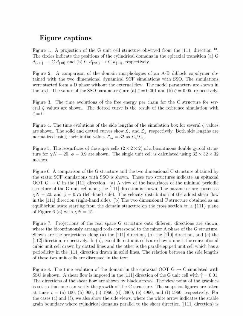
Figure captions

Figure 1. A projection of the G unit cell structure observed from the [111] direction 13.The circles indicate the positions of the cylindrical domains in the epitaxial transition (a) Gd{211} → C d{10} and (b) G d{220} → C d{10}, respectively.

Figure 2. A comparison of the domain morphologies of an A-B diblock copolymer ob-tained with the two dimensional dynamical SCF simulations with SSO. The simulationswere started form a D phase without the external flow. The model parameters are shown inthe text. The values of the SSO parameter ζ are (a) ζ = 0.001 and (b) ζ = 0.05, respectively.

Figure 3. The time evolutions of the free energy per chain for the C structure for sev-eral ζ values are shown. The dotted curve is the result of the reference simulation withζ = 0.

Figure 4. The time evolutions of the side lengths of the simulation box for several ζ valuesare shown. The solid and dotted curves show Lx and Ly, respectively. Both side lengths arenormalized using their initial values Li0 = 32 as Li/Li0 .

Figure 5. The isosurfaces of the super cells (2× 2× 2) of a bicontinous double gyroid struc-ture for χN = 20, φ = 0.9 are shown. The single unit cell is calculated using 32 × 32 × 32meshes.

Figure 6. A comparison of the G structure and the two dimensional C structure obtained bythe static SCF simulations with SSO is shown. These two structures indicate an epitaxialOOT G → C in the [111] direction. (a) A view of the isosurfaces of the minimal periodicstructure of the G unit cell along the [111] direction is shown, The parameter are chosen asχN = 20, and φ = 0.75 (left-hand side). The velocity distribution of the added shear flowin the [111] direction (right-hand side). (b) The two dimensional C structure obtained as anequilibrium state starting from the domain structure on the cross section on a {111} planeof Figure 6 (a) with χN = 15.

Figure 7. Projections of the real space G structure onto different directions are shown,where the bicontinuously arranged rods correspond to the minor A phase of the G structure.Shown are the projections along (a) the [111] direction, (b) the [110] direction, and (c) the[112] direction, respectively. In (a), two different unit cells are shown: one is the conventionalcubic unit cell drawn by dotted lines and the other is the parallelepiped unit cell which has aperiodicity in the [111] direction drawn in solid lines. The relation between the side lengthsof these two unit cells are discussed in the text.

Figure 8. The time evolution of the domain in the epitaxial OOT G → C simulated withSSO is shown. A shear flow is imposed in the [111] direction of the G unit cell with γ = 0.01.The directions of the shear flow are shown by black arrows. The view point of the graphicsis set so that one can verify the growth of the C structure. The snapshot figures are takenat times t = (a) 100, (b) 960, (c) 1960, (d) 3960, (e) 4960, and (f) 5960, respectively. Forthe cases (c) and (f), we also show the side views, where the white arrow indicates the stablegrain boundary where cylindrical domains parallel to the shear direction ([111] direction) is

generated.

Figure 9. The time evolutions of the side lengths of the simulation box during the phasetransition are shown.

Figure 10. Similar to Figure 8 but without SSO.

Figure 11. The time evolutions of the free energy per polymer chain with SSO and withoutSSO during the phase transition are shown. In both of these cases, the initial value of thefree energy is set to be zero.

Figure 12. The time evolution of the G domain under a shear flow with its velocity gra-dient in the X direction and with γ = 0.01. The circles indicate the three fold junctionperpendicularly oriented to the [111] direction of the G structure. (a) Three fold junctionsare disconnected at t=3600. (b) Three fold junctions are regenerated at t=4200.

Figure 13. Three fold junctions are migrated to different directions by the shear flow. (a)Under a shear flow with velocity gradient in the Y -direction and (b) a shear flow with veloc-ity gradient in the X-direction. In these two cases, the domains migrate in different manners.

Figure 14. The model of the kinetic pathway of the epitaxial OOT G → C is illustrated.(a) Shown is the view of the G unit cell along the [111] direction, where the black domainstransform to the C domains. (b) Another view of the same G unit cell as in (a) from adifferent direction is shown. (c) An image of the transformation from the elongated domainsto the cylinders is shown. (d) Positions of the rearranged cylinders with hexagonal order areshown, where the lattice spacings satisfy the epitaxial relations G d{220} → C d{10}.

Figure 1:

Figure 2:

Figure 3:

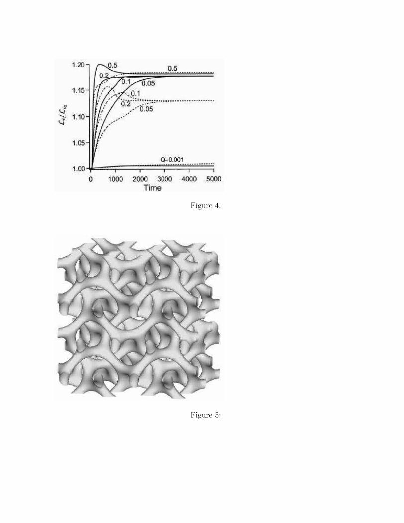
Figure 4:

Figure 5:

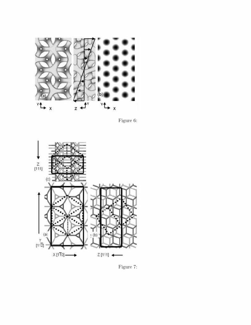
Figure 6:

Figure 7:

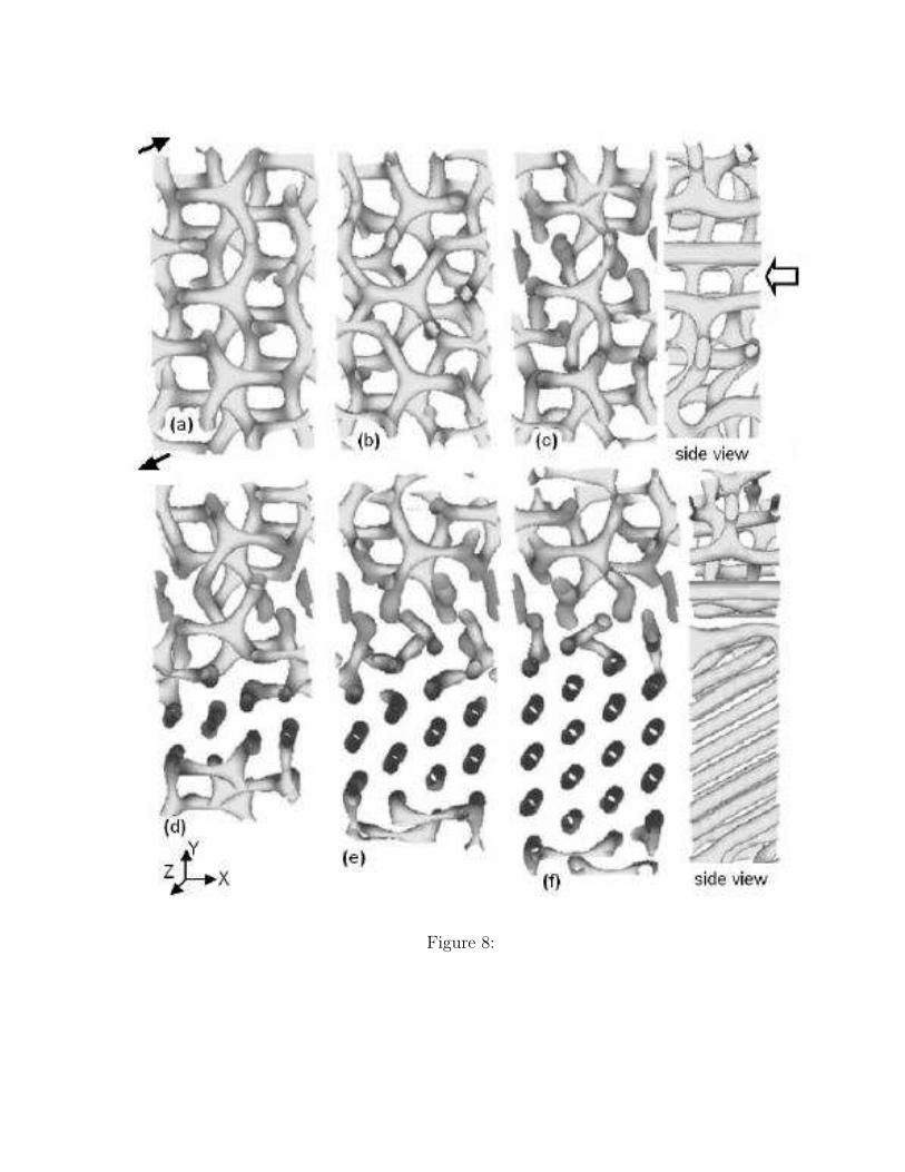
Figure 8:

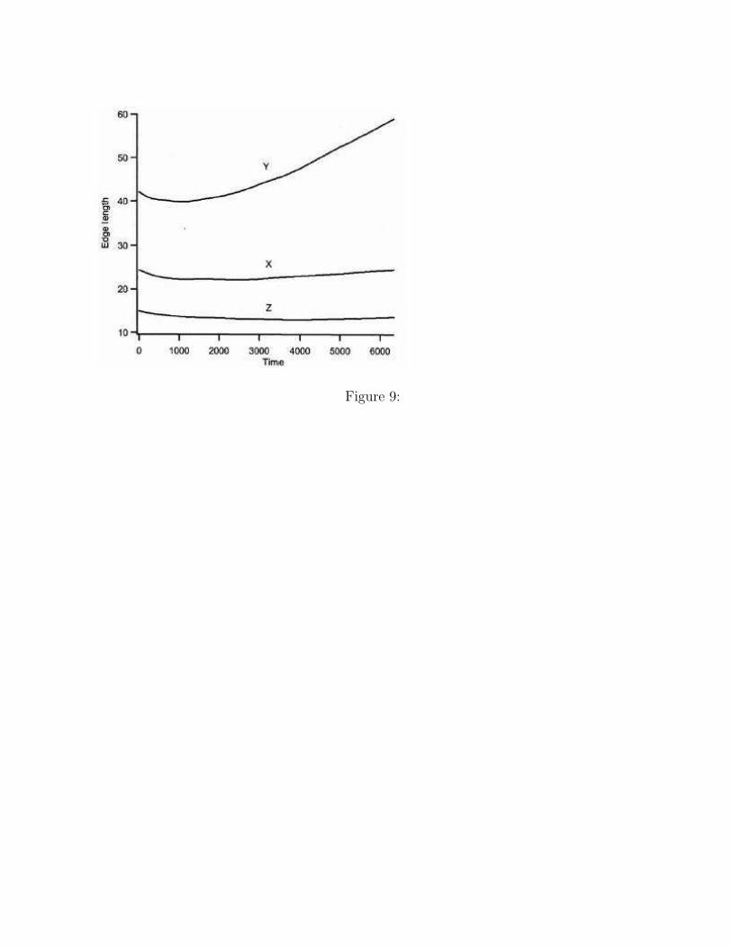
Figure 9:

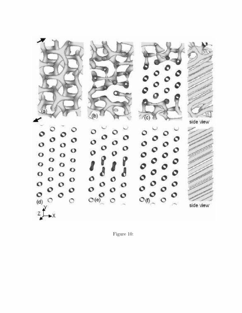
Figure 10:

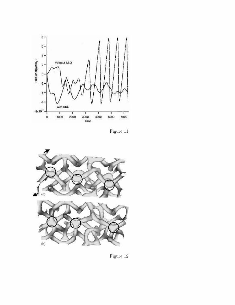
Figure 11:

Figure 12:

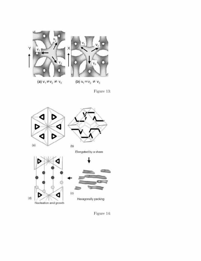
Figure 13:

Figure 14: