Epipolar Geometry

TOOLBOX

User Guide v1.3 (Dec. 2005)

Web: http://egt.dii.unisi.it

For use with MATLAB®

Gian Luca MARIOTTINI

Domenico PRATTICHIZZO

University of Siena, Siena, ITALY

2

3

An Introduction to EGT

The Epipolar Geometry Toolbox (EGT) was created to provide MATLAB users with an extensible

framework for the creation and visualization of multicamera scenarios as well as for the manipulation of the

visual information and the geometry between them. Functions provided, for both pinhole and panoramic vision

sensors, include camera placement and visualization, computation, estimation of epipolar geometry entities, and

many others. The compatibility of EGT with the Corke’s Robotics Toolbox enables users to address general

vision based control issues. The complete toolbox, detailed manual, and demo examples are freely available on

the EGT Web site (http://egt.dii.unisi.it).

This User’s Manual is aimed at helping in use EGT v1.3.

We recommend you to look below and read the “Right to use, citation…” section.

To the beginners we suggest to study first the paper “Mariottini_RAM05.pdf “, in which EGT is introduced in a

tutorial form.

Then we suggest to load and run all examples contained in the folder “demos” in order to see all the EGT

potentialities.

Related publications

• G.L. Mariottini, D. Prattichizzo "The Epipolar Geometry Toolbox: multiple view geometry and visual servoing for MATLAB", IEEE Robotics & Automation Magazine, vol. 12, Dec. 2005

• G.L. Mariottini, E.Alunno, J. Piazzi, D.Prattichizzo , "Visual Servoing with Central Catadioptric Camera", Birkhauser, 2005. (here you can find a short introduction to EGT)

• G.L. Mariottini, D.Prattichizzo, "The Epipolar Geometry Toolbox (EGT) for Matlab v1.1",

Technical Report 07-21-3-DII, University of Siena, July 2004 Siena, Italy.

Previous Versions All the previous versions can be found at http://egt.dii.unisi.it .

Compatibility EGT v1.3 is compatible with MATAB 6.5 or upper and run under Windows and Linux.

Rights to use, citation etc.

Many people are using EGT for teaching and research purposes in vision and robotics. If you plan to duplicate

the documentation for class use then every copy must include the front page of the original manual provided in

pdf format with the release.

If you want to cite EGT in your research, please use:

@ARTICLE{MariottiniPr_RAM05, AUTHOR = {G.L. Mariottini and D. Prattichizzo}, JOURNAL = {IEEE Robotics and Automation Magazine}, MONTH = {December}, NUMBER = {12}, PAGES = {}, TITLE = {EGT: a Toolbox for Multiple View Geometry and Visual Servoing}, VOLUME = {3}, YEAR = {2005} }

4

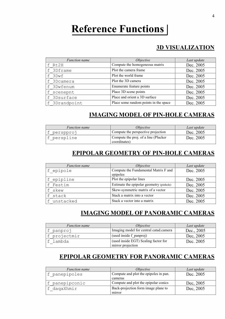
3D VISUALIZATION

Function name Objective Last update

f_Rt2H Compute the homogeneous matrix Dec. 2005

f_3Dframe Plot the camera frame Dec. 2005

f_3Dwf Plot the world frame Dec. 2005

f_3Dcamera Plot the 3D camera Dec. 2005

f_3Dwfenum Enumerate feature points Dec. 2005

f_scenepnt Place 3D scene points Dec. 2005

f_3Dsurface Place and orient a 3D surface Dec. 2005

f_3Drandpoint Place some random points in the space Dec. 2005

IMAGING MODEL OF PIN-HOLE CAMERAS

Function name Objective Last update

f_perspproj Compute the perspective projection Dec. 2005

f_perspline Compute the proj. of a line (Plucker

coordinates) Dec. 2005

EPIPOLAR GEOMETRY OF PIN-HOLE CAMERAS

Function name Objective Last update

f_epipole Compute the Fundamental Matrix F and

epipoles Dec. 2005

f_epipline Plot the epipolar lines Dec. 2005

f_Festim Estimate the epipolar geometry (pinhole) Dec. 2005

f_skew Skew-symmetric matrix of a vector Dec. 2005

f_stack Stack a matrix into a vector Dec. 2005

f_unstacked Stack a vector into a matrix Dec. 2005

IMAGING MODEL OF PANORAMIC CAMERAS

Function name Objective Last update

f_panproj Imaging model for central catad.camera Dec., 2005

f_projectmir (used inside f_panproj) Dec, 2005

f_lambda (used inside EGT) Scaling factor for

mirror projection Dec. 2005

EPIPOLAR GEOMETRY FOR PANORAMIC CAMERAS

Function name Objective Last update

f_panepipoles Compute and plot the epipoles in pan.

cameras Dec. 2005

f_panepipconic Compute and plot the epipolar conics Dec, 2005

f_daqaXhmir Back-projection form image plane to

mirror Dec, 2005

Reference Functions

5

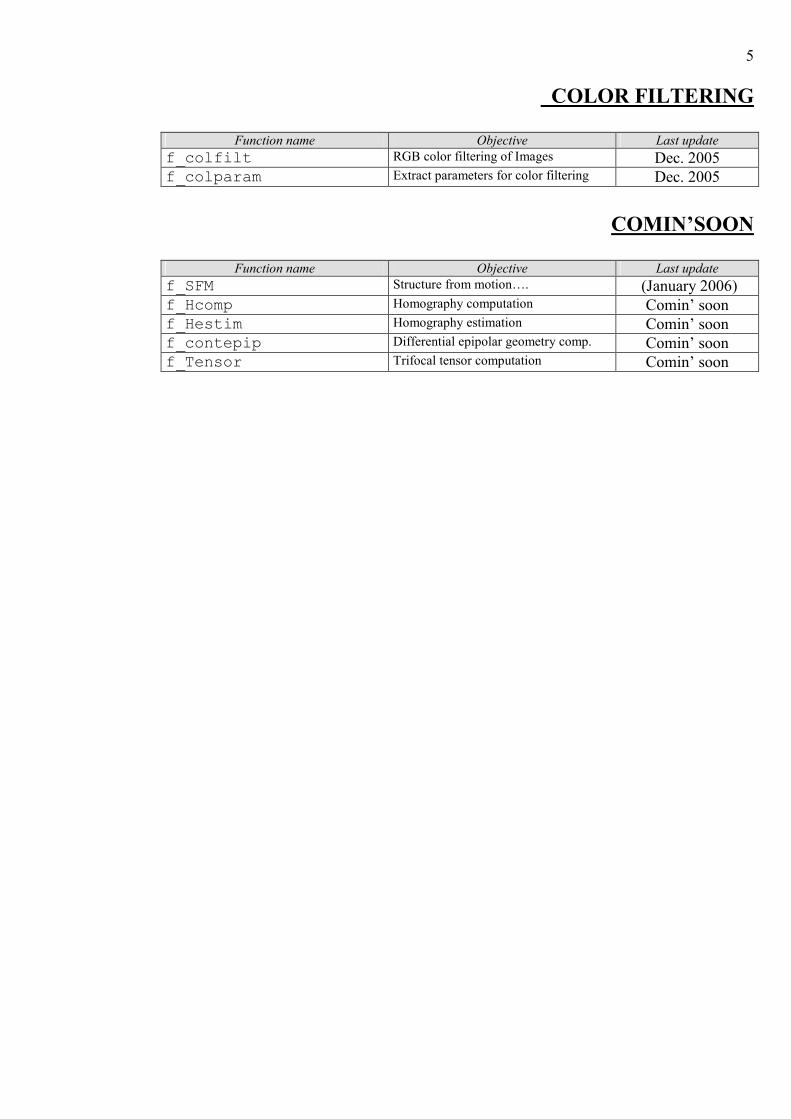
COLOR FILTERING

Function name Objective Last update

f_colfilt RGB color filtering of Images Dec. 2005

f_colparam Extract parameters for color filtering Dec. 2005

COMIN’SOON

Function name Objective Last update

f_SFM Structure from motion…. (January 2006)

f_Hcomp Homography computation Comin’ soon

f_Hestim Homography estimation Comin’ soon

f_contepip Differential epipolar geometry comp. Comin’ soon

f_Tensor Trifocal tensor computation Comin’ soon

6

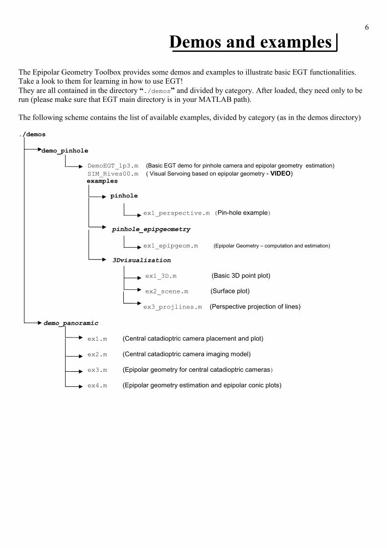
The Epipolar Geometry Toolbox provides some demos and examples to illustrate basic EGT functionalities.

Take a look to them for learning in how to use EGT!

They are all contained in the directory “./demos” and divided by category. After loaded, they need only to be

run (please make sure that EGT main directory is in your MATLAB path).

The following scheme contains the list of available examples, divided by category (as in the demos directory)

./demos

demo_pinhole

DemoEGT_1p3.m (Basic EGT demo for pinhole camera and epipolar geometry estimation)

SIM_Rives00.m ( Visual Servoing based on epipolar geometry - VIDEO) examples pinhole

ex1_perspective.m (Pin-hole example)

pinhole_epipgeometry

ex1_epipgeom.m (Epipolar Geometry – computation and estimation)

3Dvisualization

ex1_3D.m (Basic 3D point plot)

ex2_scene.m (Surface plot)

ex3_projlines.m (Perspective projection of lines)

demo_panoramic

ex1.m (Central catadioptric camera placement and plot)

ex2.m (Central catadioptric camera imaging model)

ex3.m (Epipolar geometry for central catadioptric cameras)

ex4.m (Epipolar geometry estimation and epipolar conic plots)

Demos and examples Demos and examples

7

f_Rt2H

Purpose

This function computes the 4x4 homogeneous

transformation H with respect to a rotation matrix R

and a translation vector t.

Syntax H=f_Rt2H(R,t);

Description

The input is the translational vector t centered at the world-frame and pointing toward the camera-frame.

The matrix R is the roll-pitch-yaw matrix to align the

camera-frame to the world-frame.

The world-frame is coincident with the MATLAB

frame.

The output is the homogeneous transformation 4x4

matrix H, containing the vector t and the rotation matrix

relating camera frame and world frame.

Example H1=f_Rt2H(eye(3),[0,0,0]’);

8

f_3Dwf

Purpose

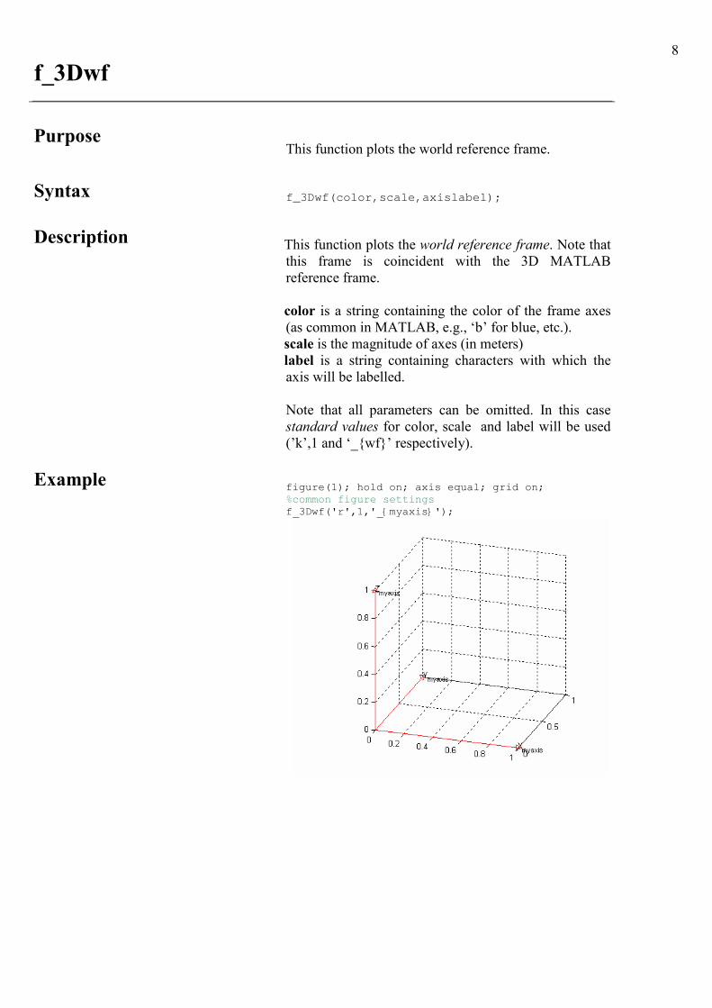
This function plots the world reference frame.

Syntax f_3Dwf(color,scale,axislabel);

Description

This function plots the world reference frame. Note that

this frame is coincident with the 3D MATLAB

reference frame.

color is a string containing the color of the frame axes

(as common in MATLAB, e.g., ‘b’ for blue, etc.).

scale is the magnitude of axes (in meters)

label is a string containing characters with which the

axis will be labelled.

Note that all parameters can be omitted. In this case

standard values for color, scale and label will be used

(’k’,1 and ‘_{wf}’ respectively).

Example figure(1); hold on; axis equal; grid on; %common figure settings f_3Dwf('r',1,'_{myaxis}');

f_3Dframe

Purpose

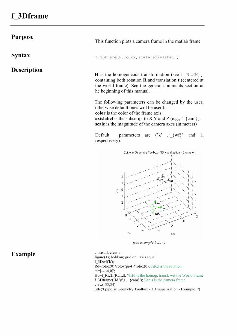
This function plots a camera frame in the matlab frame.

Syntax

f_3Dframe(H,color,scale,axislabel);

Description

H is the homogeneous transformation (see f_Rt2H), containing both rotation R and translation t (centered at

the world frame). See the general comments section at

he beginning of this manual.

The following parameters can be changed by the user,

otherwise default ones will be used):

color is the color of the frame axis.

axislabel is the subscript to X,Y and Z (e.g., ‘_{cam}).

scale is the magnitude of the camera axes (in meters)

Default parameters are (’k’ ,‘_{wf}’ and 1,

respectively).

(see example below)

Example close all; clear all

figure(1); hold on; grid on; axis equal

f_3Dwf('k');

Rd=rotoz(0)*rotoy(pi/4)*rotox(0); %Rd is the rotation

td=[-4,-4,0]';

Hd=f_Rt2H(Rd,td); %Hd is the homog. transf. wrt the World Frame

f_3Dframe(Hd,'g',1,'_{cam}'); %this is the camera frame

view(-33,34);

title('Epipolar Geometry Toolbox - 3D visualization - Example 1')

10

f_3Dcamera

Purpose

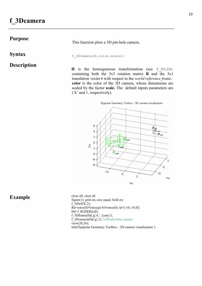
This function plots a 3D pin-hole camera.

Syntax f_3Dcamera(H,color,scale);

Description

H is the homogeneous transformation (see f_Rt2H) containing both the 3x3 rotation matrix R and the 3x1

translation vector t with respect to the world reference frame.

color is the color of the 3D camera, whose dimensions are

scaled by the factor scale. The default inputs parameters are

(’k’ and 1, respectively).

Example close all; clear all

figure(1); grid on; axis equal; hold on;

f_3Dwf('k',2);

Rd=rotoz(0)*rotoy(pi/4)*rotox(0); td=[-10,-10,0]';

Hd=f_Rt2H(Rd,td);

f_3Dframe(Hd,'g',4,'_{cam}');

f_3Dcamera(Hd,'g',1); %3D pin-hole camera

view(20,26);

title('Epipolar Geometry Toolbox - 3D camera visualization ')

11

f_3Dwfenum

Purpose

This function plots the number of feature points in the world

frame.

Syntax f_3Dwfenum(P);

Description

P is the 3xN matrix containing the feature points (expressed

in the world frame)

Example

P=[1 2; 1 3; 1 4;];

f_3Dwfenum(P);

12

(1)

(2)

(3)

(4)

(5)

(6)

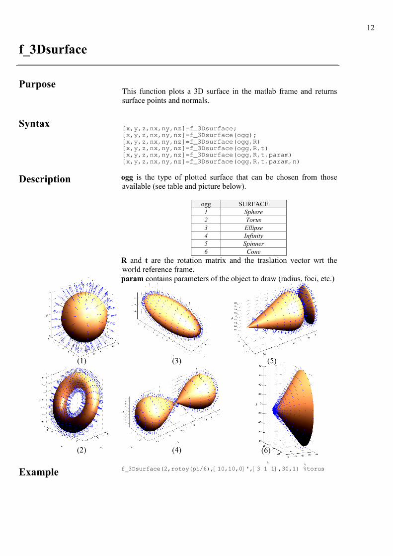
f_3Dsurface

Purpose

This function plots a 3D surface in the matlab frame and returns

surface points and normals.

Syntax [x,y,z,nx,ny,nz]=f_3Dsurface; [x,y,z,nx,ny,nz]=f_3Dsurface(ogg); [x,y,z,nx,ny,nz]=f_3Dsurface(ogg,R) [x,y,z,nx,ny,nz]=f_3Dsurface(ogg,R,t) [x,y,z,nx,ny,nz]=f_3Dsurface(ogg,R,t,param) [x,y,z,nx,ny,nz]=f_3Dsurface(ogg,R,t,param,n)

Description ogg is the type of plotted surface that can be chosen from those

available (see table and picture below).

ogg SURFACE

1 Sphere

2 Torus

3 Ellipse

4 Infinity

5 Spinner

6 Cone

R and t are the rotation matrix and the traslation vector wrt the

world reference frame.

param contains parameters of the object to draw (radius, foci, etc.)

Example f_3Dsurface(2,rotoy(pi/6),[10,10,0]',[3 1 1],30,1) %torus

13

f_scenepnt

Purpose

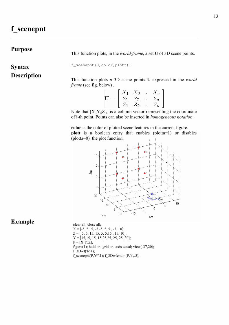
This function plots, in the world-frame, a set U of 3D scene points.

Syntax f_scenepnt(U,color,plott);

Description

This function plots n 3D scene points U expressed in the world

frame (see fig. below) .

Note that [Xi;Yi;Z i] is a column vector representing the coordinate

of i-th point. Points can also be inserted in homogeneous notation.

color is the color of plotted scene features in the current figure.

plott is a boolean entry that enables (plotta=1) or disables

(plotta=0) the plot function.

Example

clear all; close all;

X = [-5, 5, 5, -5,-5, 5, 5 , -5, 10];

Z = [ 5, 5, 15, 15, 5, 5,15 , 15, 10];

Y = [15,15, 15, 15,25,25, 25, 25, 30];

P = [X;Y;Z];

figure(1); hold on; grid on; axis equal; view(-37,20);

f_3Dwf('b',4);

f_scenepnt(P,'r*',1); f_3Dwfenum(P,'k',.5);

14

f_3Drandpoint

Purpose

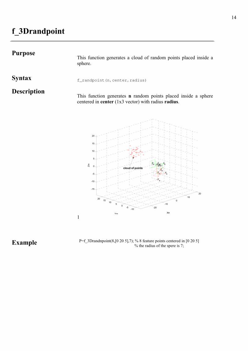
This function generates a cloud of random points placed inside a

sphere.

Syntax f_randpoint(n,center,radius)

Description

This function generates n random points placed inside a sphere

centered in center (1x3 vector) with radius radius.

-20

-10

0

10

20

-10-5

05

1015

20

-15

-10

-5

0

5

10

15

20

Xm

Xa

Xd

Za

Xw f

Zw f

Yd

Ya

Yw f

Zd

Ym

Zm

cloud of points

1

Example P=f_3Drandnpoint(8,[0 20 5],7); % 8 feature points centered in [0 20 5]

% the radius of the spere is 7;

15

f_perspproj

Purpose

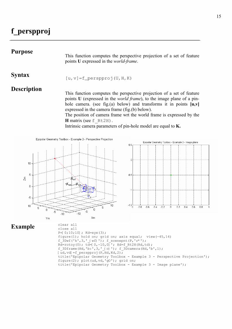
This function computes the perspective projection of a set of feature

points U expressed in the world-frame.

Syntax [u,v]=f_perspproj(U,H,K)

Description

This function computes the perspective projection of a set of feature

points U (expressed in the world frame), to the image plane of a pin-

hole camera. (see fig.(a) below) and transforms it in points [u,v]

expressed in the camera frame (fig.(b) below).

The position of camera frame wrt the world frame is expressed by the

H matrix (see f_Rt2H). Intrinsic camera parameters of pin-hole model are equal to K.

Example clear all close all P=[0;10;10]; Kd=eye(3); figure(1); hold on; grid on; axis equal; view(-45,14) f_3Dwf('k',3,'_{wf}'); f_scenepnt(P,'r*'); Rd=rotoy(0); td=[0,-10,0]'; Hd=f_Rt2H(Rd,td); f_3Dframe(Hd,'b:',3,'_{c}'); f_3Dcamera(Hd,'b',1); [ud,vd]=f_perspproj(P,Hd,Kd,2); title('Epipolar Geometry Toolbox - Example 3 - Perspective Projection'); figure(2); plot(ud,vd,'gO'); grid on; title('Epipolar Geometry Toolbox - Example 3 - Image plane');

16

f_epipole

Purpose

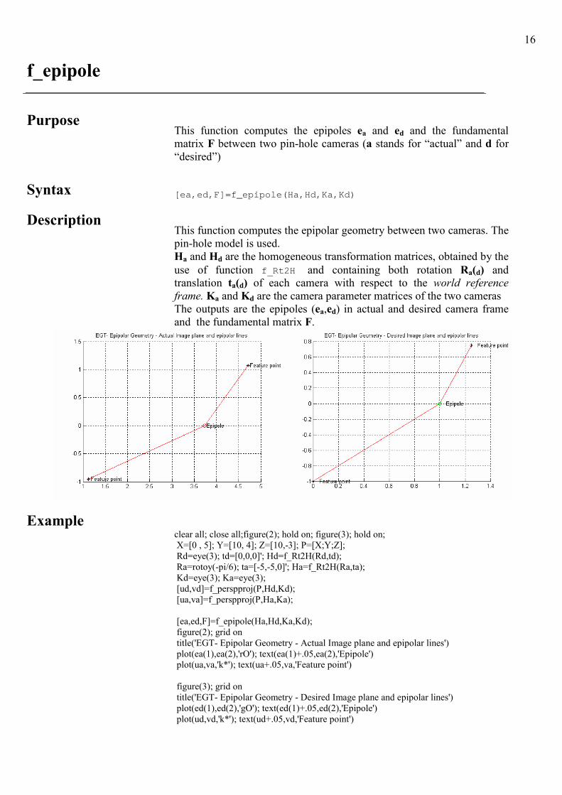
This function computes the epipoles ea and ed and the fundamental

matrix F between two pin-hole cameras (a stands for “actual” and d for

“desired”)

Syntax [ea,ed,F]=f_epipole(Ha,Hd,Ka,Kd)

Description

This function computes the epipolar geometry between two cameras. The

pin-hole model is used.

Ha and Hd are the homogeneous transformation matrices, obtained by the

use of function f_Rt2H and containing both rotation Ra(d) and

translation ta(d) of each camera with respect to the world reference

frame. Ka and Kd are the camera parameter matrices of the two cameras

The outputs are the epipoles (ea,ed) in actual and desired camera frame

and the fundamental matrix F.

Example

clear all; close all;figure(2); hold on; figure(3); hold on;

X=[0 , 5]; Y=[10, 4]; Z=[10,-3]; P=[X;Y;Z];

Rd=eye(3); td=[0,0,0]'; Hd=f_Rt2H(Rd,td);

Ra=rotoy(-pi/6); ta=[-5,-5,0]'; Ha=f_Rt2H(Ra,ta);

Kd=eye(3); Ka=eye(3);

[ud,vd]=f_perspproj(P,Hd,Kd);

[ua,va]=f_perspproj(P,Ha,Ka);

[ea,ed,F]=f_epipole(Ha,Hd,Ka,Kd);

figure(2); grid on

title('EGT- Epipolar Geometry - Actual Image plane and epipolar lines')

plot(ea(1),ea(2),'rO'); text(ea(1)+.05,ea(2),'Epipole')

plot(ua,va,'k*'); text(ua+.05,va,'Feature point')

figure(3); grid on

title('EGT- Epipolar Geometry - Desired Image plane and epipolar lines')

plot(ed(1),ed(2),'gO'); text(ed(1)+.05,ed(2),'Epipole')

plot(ud,vd,'k*'); text(ud+.05,vd,'Feature point')

17

f_epipline

Purpose

This function computes and plots the epipolar lines pencil.

Syntax [la,ld]=f_epipline(Ua,Ud,F,flag,fig_a,fig_d,car);

Description

Example

This function computes and plots the pencil of epipolar lines. The

pin-hole model is used.

The input is the set of corresponding points Ua and Ud in the first and

second views, respectively (they can also be expressed in

homogeneous notation).

The fundamental matrix F is also required as to compute the epipolar

line:

Where xd (xa) corresponds to a column (i.e., only a point) in the Ud

(Ua) matrix. flag is a boolean variable and indicates that all plot

functionalities are enabled (flag=1) or disabled (flag=0).

fig_a and fig_d are integers and represent the indexes of the figures

where to plot epipolar lines (for both the first and the second views

respectively). car is the string containing color and shape of lines

(i.e. car=’r:’ for dotted red epipolar line).

clear all; close all; figure(2); hold on; figure(3); hold on;

X=[0 , 5]; Y=[10, 4]; Z=[10,-3]; P=[X;Y;Z];

Rd=eye(3); td=[0,0,0]'; Hd=f_Rt2H(Rd,td);

Ra=rotoy(-pi/6); ta=[-5,-5,0]'; Ha=f_Rt2H(Ra,ta);

Kd=eye(3); Ka=eye(3);

[ud,vd]=f_perspproj(P,Hd,Kd);

[ua,va]=f_perspproj(P,Ha,Ka);

[ea,ed,F]=f_epipole(Ha,Hd,Ka,Kd);

figure(2); grid on

title('EGT- Epipolar Geometry - Actual Image plane and epipolar lines')

plot(ea(1),ea(2),'rO'); text(ea(1)+.05,ea(2),'Epipole')

plot(ua,va,'k*'); text(ua+.05,va,'Feature point')

figure(3); grid on

title('EGT- Epipolar Geometry - Desired Image plane and epipolar lines')

plot(ed(1),ed(2),'gO'); text(ed(1)+.05,ed(2),'Epipole')

plot(ud,vd,'k*'); text(ud+.05,vd,'Feature point')

Ua=[ua;va]; Ud=[ud;vd];

[la,ld]=f_epipline(Ua,Ud,F);

18

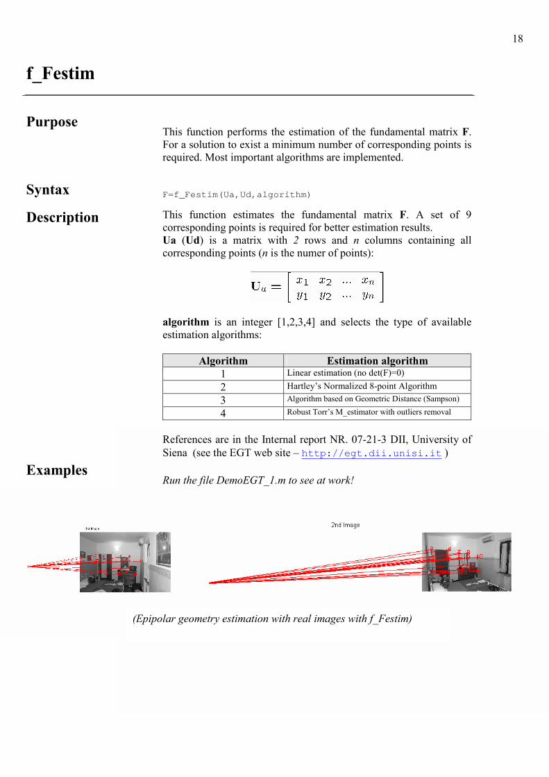
f_Festim

Purpose

This function performs the estimation of the fundamental matrix F.

For a solution to exist a minimum number of corresponding points is

required. Most important algorithms are implemented.

Syntax F=f_Festim(Ua,Ud,algorithm)

Description

This function estimates the fundamental matrix F. A set of 9

corresponding points is required for better estimation results.

Ua (Ud) is a matrix with 2 rows and n columns containing all

corresponding points (n is the numer of points):

algorithm is an integer [1,2,3,4] and selects the type of available

estimation algorithms:

Algorithm Estimation algorithm

1 Linear estimation (no det(F)=0)

2 Hartley’s Normalized 8-point Algorithm

3 Algorithm based on Geometric Distance (Sampson)

4 Robust Torr’s M_estimator with outliers removal

References are in the Internal report NR. 07-21-3 DII, University of

Siena (see the EGT web site – http://egt.dii.unisi.it )

Examples

Run the file DemoEGT_1.m to see at work!

(Epipolar geometry estimation with real images with f_Festim)

19

f_normalize

Purpose

This function normalizes feature points (in image plane). This

normalization has been introduced by Hartley in his “8 point

algorithm” in order to obtain a better fundamental matrix estimation.

Syntax [Unorm,T]=f_normalize(U)

Description

This function performs a transformation T that normalizes feature

points (in image plane). This is needed for many algorithms (such as

the Hartley’s 8 point algorithm) in order to obtain a better

fundamental matrix estimation. It consists of a translation and a

scaling of each image point so that the centroid of the reference

points is at the origin of the coordinates and the RMS distance of the

points from the origin is equal to sqrt(2).

The normalized coordinates Unorm of points are given as output

together with the transformation matrix T.

20

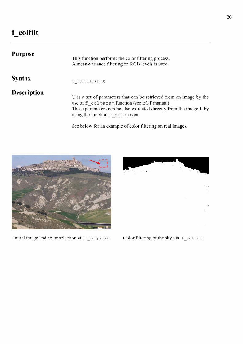
f_colfilt

Purpose

This function performs the color filtering process.

A mean-variance filtering on RGB levels is used.

Syntax f_colfilt(I,U)

Description

U is a set of parameters that can be retrieved from an image by the

use of f_colparam function (see EGT manual). These parameters can be also extracted directly from the image I, by

using the function f_colparam.

See below for an example of color filtering on real images.

Initial image and color selection via f_colparam Color filtering of the sky via f_colfilt

21

f_colparam

Purpose This function aims to extract color parameters (mean-variance) by

clicking on a point or by cropping an area of the color image I. These

parameters are needed in f_colfilt function.

Syntax U=f_colparam(I,flag,type);

Description

Computation of color parameters for color filtering.

The function takes as input an image I and enables the user to click (type=1) or to crop (type=2) an image section. Pixels will be used to

compute mean and variance.

I= rgb image (acquired via imread of MATLAB) flag = use adaptive or not technique for sigma computation

type = 1 � clicking

type = 2 � croping

flag = 1 � not adaptive

flag = 2 � adaptive

and where

U= [mr mg mb vr vg vb sigma_r sigma_g sigma_b]

22

f_perspline

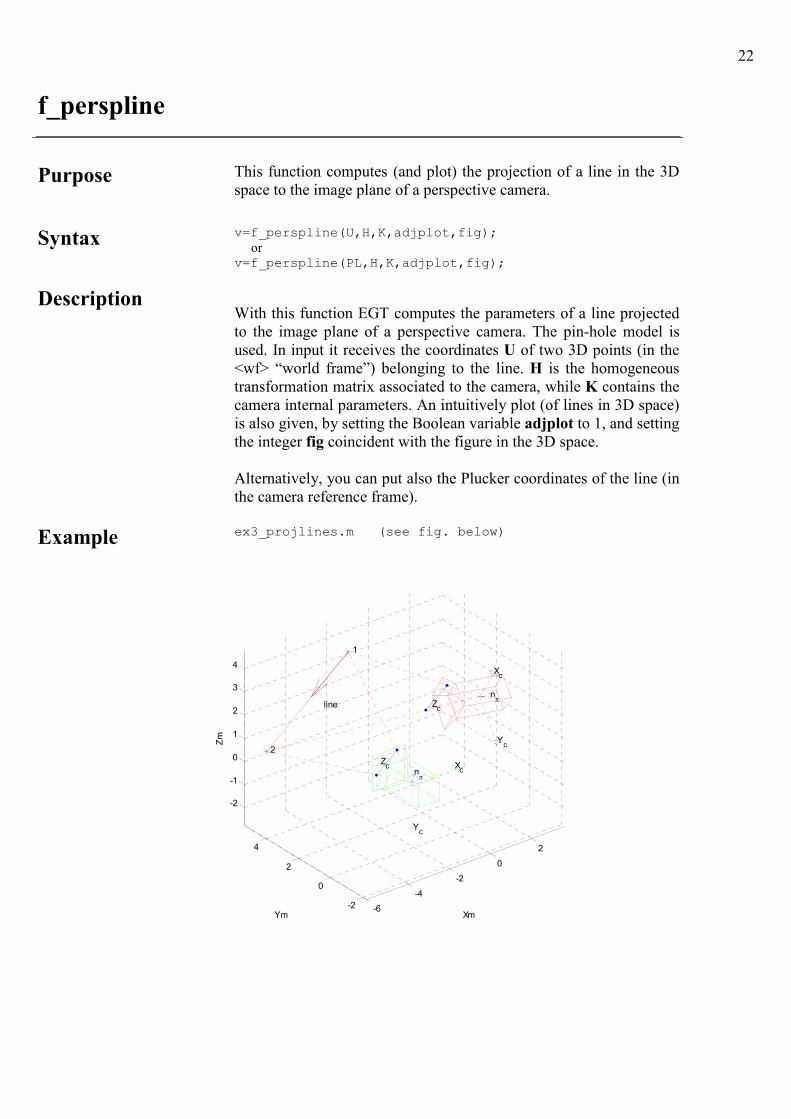
Purpose This function computes (and plot) the projection of a line in the 3D

space to the image plane of a perspective camera.

Syntax v=f_perspline(U,H,K,adjplot,fig); or v=f_perspline(PL,H,K,adjplot,fig);

Description

With this function EGT computes the parameters of a line projected

to the image plane of a perspective camera. The pin-hole model is

used. In input it receives the coordinates U of two 3D points (in the

<wf> “world frame”) belonging to the line. H is the homogeneous

transformation matrix associated to the camera, while K contains the

camera internal parameters. An intuitively plot (of lines in 3D space)

is also given, by setting the Boolean variable adjplot to 1, and setting

the integer fig coincident with the figure in the 3D space.

Alternatively, you can put also the Plucker coordinates of the line (in

the camera reference frame).

Example ex3_projlines.m (see fig. below)

-6

-4

-2

0

2

-2

0

2

4

-2

-1

0

1

2

3

4

Yc

Xc

nπ

Xm

Xc

Zc

nπ

Yc

Zc

1

Ym

2

Zm

line

23

f_3Dpanoramic

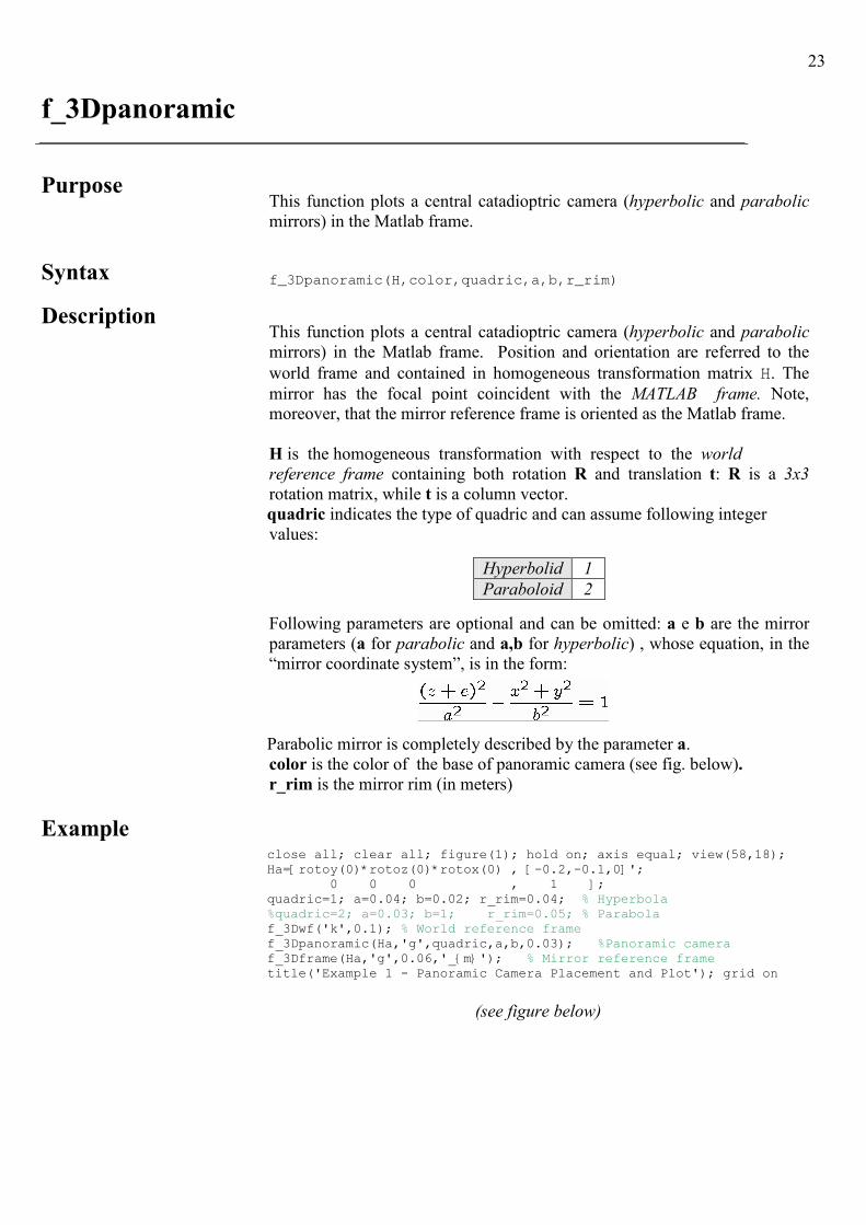
Purpose

This function plots a central catadioptric camera (hyperbolic and parabolic

mirrors) in the Matlab frame.

Syntax f_3Dpanoramic(H,color,quadric,a,b,r_rim)

Description

This function plots a central catadioptric camera (hyperbolic and parabolic

mirrors) in the Matlab frame. Position and orientation are referred to the

world frame and contained in homogeneous transformation matrix H. The mirror has the focal point coincident with the MATLAB frame. Note,

moreover, that the mirror reference frame is oriented as the Matlab frame.

H is the homogeneous transformation with respect to the world

reference frame containing both rotation R and translation t: R is a 3x3

rotation matrix, while t is a column vector.

quadric indicates the type of quadric and can assume following integer

values:

Hyperbolid 1

Paraboloid 2

Following parameters are optional and can be omitted: a e b are the mirror

parameters (a for parabolic and a,b for hyperbolic) , whose equation, in the

“mirror coordinate system”, is in the form:

Parabolic mirror is completely described by the parameter a.

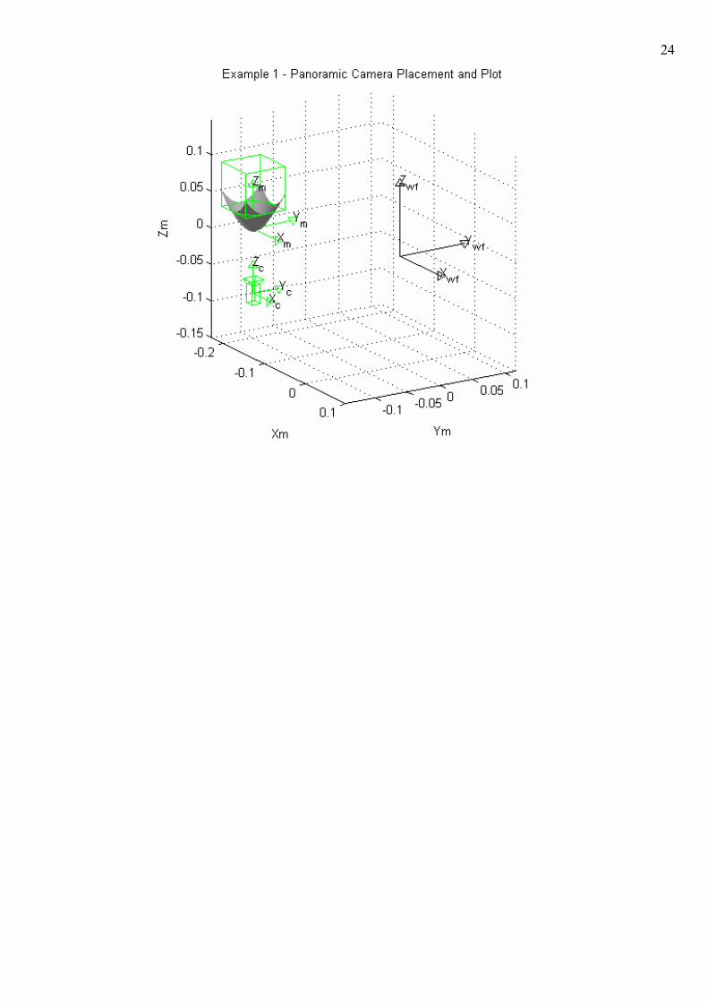
color is the color of the base of panoramic camera (see fig. below).

r_rim is the mirror rim (in meters)

Example close all; clear all; figure(1); hold on; axis equal; view(58,18); Ha=[rotoy(0)*rotoz(0)*rotox(0) , [-0.2,-0.1,0]'; 0 0 0 , 1 ]; quadric=1; a=0.04; b=0.02; r_rim=0.04; % Hyperbola %quadric=2; a=0.03; b=1; r_rim=0.05; % Parabola f_3Dwf('k',0.1); % World reference frame f_3Dpanoramic(Ha,'g',quadric,a,b,0.03); %Panoramic camera f_3Dframe(Ha,'g',0.06,'_{m}'); % Mirror reference frame title('Example 1 - Panoramic Camera Placement and Plot'); grid on

(see figure below)

24

25

f_projectmir

Purpose

Central catadioptric projection of a point onto the mirror surface

(referred to the mirror frame). This function is mainly used inside other functions of EGT.

Syntax pmir = f_projectmir(a,b,quadric,Xmir);

Description

A central catadioptric projection is made by two steps: first, the

world point X is projected by a central projection to the point x in

the mirror surface.

Second, the point on the mirror surface is then projected to the

image plane of conventional camera.

Here the first step is implemented.

a, b are the hyperbolic mirror parameters of the panoramic camera.

Xmir is a 3xn matrix containing all n scene points (each point is a

3x1 column vector) in the mirror frame. The function returns the

column vector pmir, i.e. the coordinates of the projection onto the

mirror surface.

26

f_lambda

Purpose

Scaling factors defining the intersections between a two sheet

hyperboloid of revolution and a line going from the origin to a

scene point. This function is mainly used inside other functions of EGT.

Syntax [lambda1,lambda2] = f_lambda(a,b,quadric,v);

Description

This function returns the scale factors, 1λ and 2λ , which define the

intersections between a mirror (hyperbolid/paraboloid) of

revolution, with equation in the mirror frame, and a line going from

the origin of the mirror frame to a scene point v. The intersections

are defined as 1λ v and 2λ v.

a, b are the parabola(hyperboloid) mirror parameters of the mirror.

v is a column vector with no-homogeneous coordinates, expressed

in the mirror frame, of the scene point. The function outputs are

lambda1 and lambda2, i.e. the scale factors 1λ and 2λ . To obtain

the intersections we have 1λ v and 2λ v.

27

f_panproj

Purpose

This function implements the imaging model of a central

catadioptric camera with both parabolic and hyperbolic mirrors. In

particular, it projects the scene points into image points returning

both the pixel coordinates and the mirror coordinates (meters) in

CCD and mirror reference frame, respectively.

Syntax [q,Xhmir]=f_panproj(X,H,K,a,b,quadric,color)

Description

X is a 4xN (homogeneous coordinates) or 3xN matrix (no-

homogeneous coordinates ) where N is the number of points. Each

point is a column vector of X.

Following parameters are optional and can be omitted:

H is the homogeneous transformation with respect to the world

reference frame containing both rotation R and translation t.

Note that R is a 3x3 rotation matrix while t is a column vector

(centered at the world frame and pointing to the mirror focus).

K is the calibration matrix of the CCD camera. a e b are the mirror

parameters (in meters). quadric can be 1 or 2 if the mirror is a

hyperboloid or a paraboloid. color, at last, defines the color used to

plot the mirror projection of the scene points onto the mirror

surface.

The output q of f_panproj is a 2xN matrix containing the pixel coordinates of projections of the scene points. Matrix q assume the

form:

=

N

N

vvv

uuu

...

...

21

21q

Xhmir is a 3xN matrix, where each column vector contains the

coordinates, in the “mirror coordinate system”, of the mirror

projection of the scene points.

=

N

N

N

z...zz

y...yy

x...xx

21

21

21

Xhmir

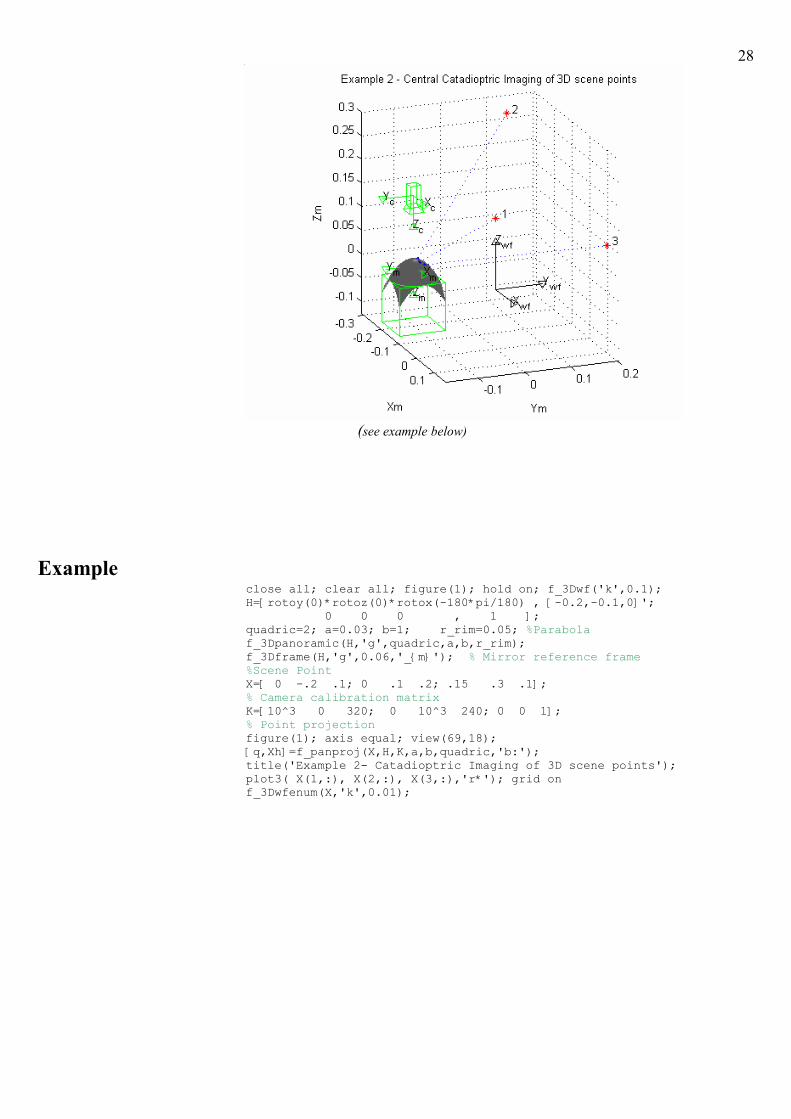
28

(see example below)

Example close all; clear all; figure(1); hold on; f_3Dwf('k',0.1); H=[rotoy(0)*rotoz(0)*rotox(-180*pi/180) , [-0.2,-0.1,0]'; 0 0 0 , 1 ]; quadric=2; a=0.03; b=1; r_rim=0.05; %Parabola f_3Dpanoramic(H,'g',quadric,a,b,r_rim); f_3Dframe(H,'g',0.06,'_{m}'); % Mirror reference frame %Scene Point X=[ 0 -.2 .1; 0 .1 .2; .15 .3 .1]; % Camera calibration matrix K=[10^3 0 320; 0 10^3 240; 0 0 1]; % Point projection figure(1); axis equal; view(69,18); [q,Xh]=f_panproj(X,H,K,a,b,quadric,'b:'); title('Example 2- Catadioptric Imaging of 3D scene points'); plot3( X(1,:), X(2,:), X(3,:),'r*'); grid on f_3Dwfenum(X,'k',0.01);

29

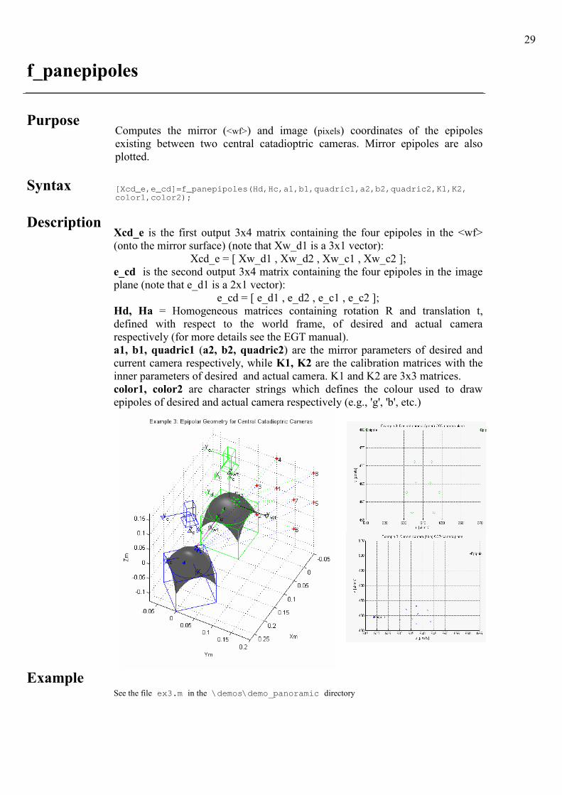
f_panepipoles

Purpose

Computes the mirror (<wf>) and image (pixels) coordinates of the epipoles

existing between two central catadioptric cameras. Mirror epipoles are also

plotted.

Syntax [Xcd_e,e_cd]=f_panepipoles(Hd,Hc,a1,b1,quadric1,a2,b2,quadric2,K1,K2, color1,color2);

Description

Xcd_e is the first output 3x4 matrix containing the four epipoles in the <wf>

(onto the mirror surface) (note that Xw_d1 is a 3x1 vector):

Xcd_e = [ Xw_d1 , Xw_d2 , Xw_c1 , Xw_c2 ];

e_cd is the second output 3x4 matrix containing the four epipoles in the image

plane (note that e_d1 is a 2x1 vector):

e_cd = [ e_d1 , e_d2 , e_c1 , e_c2 ];

Hd, Ha = Homogeneous matrices containing rotation R and translation t,

defined with respect to the world frame, of desired and actual camera

respectively (for more details see the EGT manual).

a1, b1, quadric1 (a2, b2, quadric2) are the mirror parameters of desired and

current camera respectively, while K1, K2 are the calibration matrices with the

inner parameters of desired and actual camera. K1 and K2 are 3x3 matrices.

color1, color2 are character strings which defines the colour used to draw

epipoles of desired and actual camera respectively (e.g., 'g', 'b', etc.)

Example

See the file ex3.m in the \demos\demo_panoramic directory

30

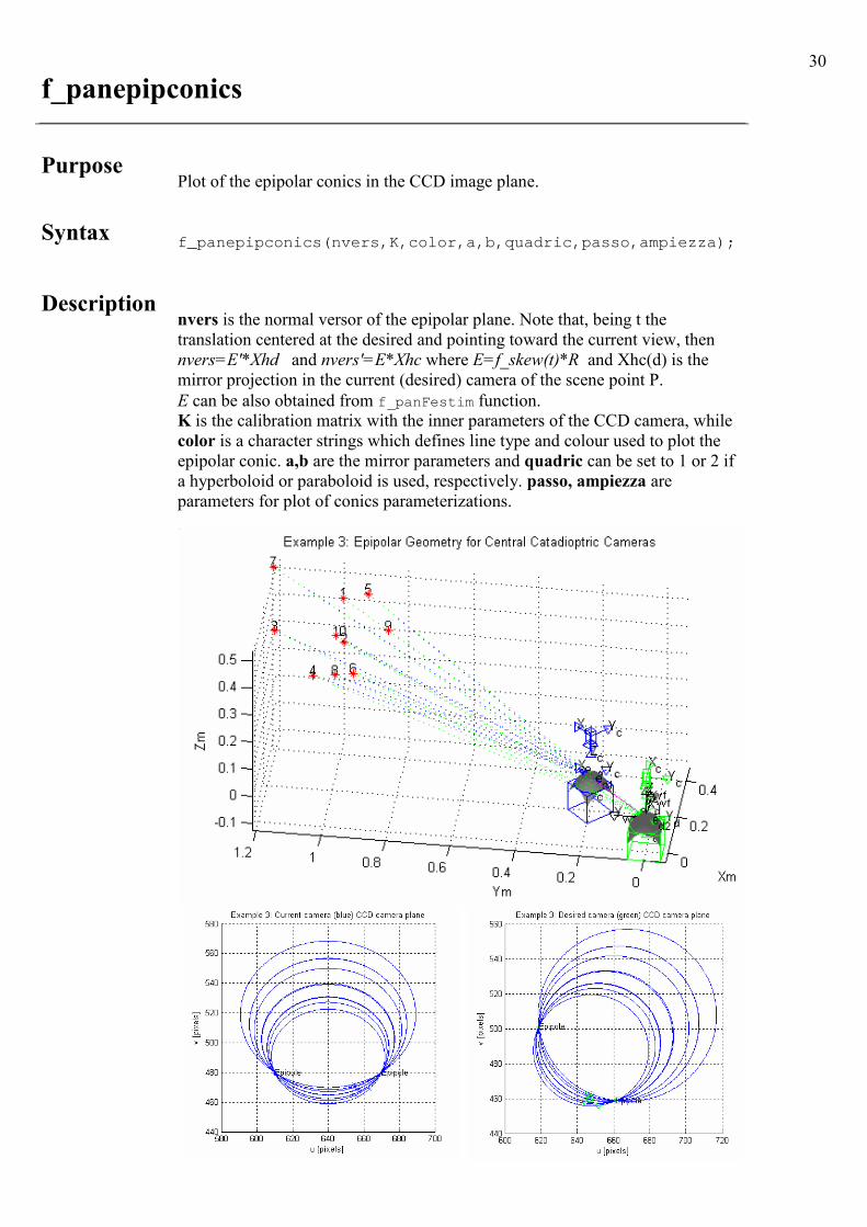
f_panepipconics

Purpose

Plot of the epipolar conics in the CCD image plane.

Syntax

f_panepipconics(nvers,K,color,a,b,quadric,passo,ampiezza);

Description

nvers is the normal versor of the epipolar plane. Note that, being t the

translation centered at the desired and pointing toward the current view, then

nvers=E'*Xhd and nvers'=E*Xhc where E=f_skew(t)*R and Xhc(d) is the

mirror projection in the current (desired) camera of the scene point P.

E can be also obtained from f_panFestim function.

K is the calibration matrix with the inner parameters of the CCD camera, while

color is a character strings which defines line type and colour used to plot the

epipolar conic. a,b are the mirror parameters and quadric can be set to 1 or 2 if

a hyperboloid or paraboloid is used, respectively. passo, ampiezza are

parameters for plot of conics parameterizations.

31

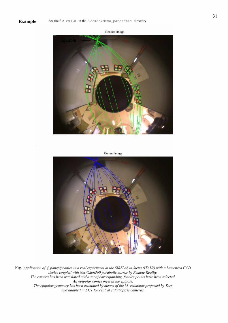
Example See the file ex4.m in the \demos\demo_panoramic directory

Fig. Application of f_panepipconics in a real experiment at the SIRSLab in Siena (ITALY) with a Lumenera CCD device coupled with NetVision360 parabolic mirror by Remote Reality.

The camera has been translated and a set of corresponding feature points have been selected.

All epipolar conics meet at the epipole.

The epipolar geometry has been estimated by means of the M- estimator proposed by Torr

and adapted in EGT for central catadioptric cameras.

32

f_daqaXhmir

Purpose

This function back-projects the image points Q (given in pixel

coordinates and obtained through a central catadioptric camera)

into mirror points Xhmir, and returns the coordinates of these ones

expressed in the mirror coordinate system.

Syntax [Xhmir] = f_daqaXhmir(Q,K,a,b,quadric);

Description

Q is a 3-by-n matrix (if the points are in homogeneous coordinates)

or 2-by-n matrix (no homogeneous coordinates) with image points

(pixel coordinates) to reproject. K is the camera calibration matrix

with the internal parameters of the camera. K is a 3by3 matrix. For

default K is equal to identity. a,b are the mirror parameters

(scalar). If no specified, default values are a = 3 cm and b = 1 cm.

33

f_conics

Purpose

Plot of conics.

Syntax flag=f_conics(A,color,passo,ampiezza);

Description

Input:

Output:

This function permits to plot regular conics. In case of singular

conic the plot is not available but it is displayed a message in the

matlab command window with the type of conic.

A conic is understood as the locus of 2D points [ ]Tyx, which

satisfy the following quadratic equation:

022 =+++++ feydycxbxyax

This quadratic form can be rewritten in the matrix form 0=AxxT ,

where A is a symmetric 3by3 matrix

=

fec

edb

cba

2/2/

2/2/

2/2/

A

and [ ]Tyx 1,,=x .

A is the symmetric matrix which defines the conic.

color, at last, is the character string which defines the colour used

to draw the conic. passo and ampiezza are parameterization

parameters of the conics

The output of the function is a flag (flag) whose value specify if

the conic are singular or no:

flag = 0 � regular conic

flag = 1 � singular conic:

two imaginary lines with a real intersection

flag = 2 � singular conic: two transverses

flag = 3 � singular conic: two parallel lines

Example A = [3 2 1; 2 2 3; 1 3 1]; f_conics(A,1,'b');

34

f_ellipse

Purpose

Parameterization of an ellipse in the essential position.

Syntax [x,y] = f_ellipse(A);

Description

This function permits to calculate the parameterization of an ellipse

in the essential position. The known form of an ellipse equation, in

the essential position is:

12

2

2

2

=+b

y

a

x

and the parameterization returned by the function is

[ ] [ ]tbtayx sin,cos, −= where π20 ≤≤ t .

A is the 3x3 symmetric matrix associated with the ellipse in the

essential position, and has the form

In x and y, the function returns the parameterization of the ellipse.

35

f_hyperbola

Purpose

Parameterization of a hyperbola in the essential position.

Syntax [x,y] = f_hyperbola(A);

Description

This function permits to calculate the parameterization of a

hyperbola in the essential position. The known form of a hyperbola

equation, in the essential position is:

12

2

2

2

=−b

y

a

x

and the parameterization returned by the function is

[ ]

+±=

2

2

1,,b

tatyx

where the parameter t is bounded by the image resolution.

A is the 3x3 symmetric matrix associated with the hyperbola in the

essential position.

In x and y, the function returns the parameterization of the

hyperbola.

36

f_parabola

Purpose

Parameterization of a parabola in the essential position.

Syntax [x,y] = f_parabola(A);

Description

This function permits to calculate the parameterization of a

parabola in the essential position. The known form of a parabola

equation, in the essential position is:

2axy = or 2ayx =

and the parameterization returned by the function is

[ ]

−= 2

23

11

2,, ta

atyx or [ ]

−= tta

ayx ,

2, 2

13

22

where the parameter t is bounded by the image resolution.

A is the 3x3 symmetric matrix associated with the parabola in the

essential position.

In x and y, the function returns the parameterization of the

parabola.