Embed Size (px)
Citation preview
Integrated causal-predictive machine learning models for tropical cyclone
epidemiology
Rachel C. Nethery1, Nina Katz-Christy2, Marianthi-Anna Kioumourtzoglou3,
Robbie M. Parks3, Andrea Schumacher4, G. Brooke Anderson5
1Department of Biostatistics, Harvard T.H. Chan School of Public Health2Department of Statistics, Harvard University, Faculty of Arts and Sciences
3Department of Environmental Health Sciences, Columbia Mailman School of Public Health4Cooperative Institute for Research in the Atmosphere, Colorado State University
5Department of Environmental & Radiological Health Sciences, Colorado State University
Abstract
Strategic preparedness has been shown to reduce the adverse health impacts of hurricanes and tropi-cal storms, referred to collectively as tropical cyclones (TCs), but its protective impact could be enhancedby a more comprehensive and rigorous characterization of TC epidemiology. To generate the insightsand tools necessary for high-precision TC preparedness, we develop and apply a novel Bayesian machinelearning approach that standardizes estimation of historic TC health impacts, discovers common pat-terns and sources of heterogeneity in those health impacts, and enables identification of communities athighest health risk for future TCs. The model integrates (1) a causal inference component to quantifythe immediate health impacts of recent historic TCs at high spatial resolution and (2) a predictive com-ponent that captures how TC meteorological features and socioeconomic/demographic characteristicsof impacted communities are associated with health impacts. We apply it to a rich data platform con-taining detailed historic TC exposure information and Medicare claims data. The health outcomes usedin our analyses are all-cause mortality and cardiovascular- and respiratory-related hospitalizations. Wereport a high degree of heterogeneity in the acute health impacts of historic TCs at both the TC leveland the community level, with substantial increases in respiratory hospitalizations, on average, duringa two-week period surrounding TCs. TC sustained windspeeds are found to be the primary driver ofincreased mortality and respiratory risk. Our modeling approach has broader utility for predicting thehealth impacts of many types of extreme climate events.
1 Introduction
The US National Oceanic and Atmospheric Administration reports that tropical cyclones (TCs) imposethe largest financial burden of any weather disasters in the US, costing $945.9 billion since 1980 or roughly$21.5 billion per event (National Oceanic and Atmospheric Administration, 2020). TCs, which includehurricanes and tropical storms, often bring severe winds, rainfall, and flooding (Shultz et al., 2005), whichcan catalyze massive property and infrastructure damage. Due to the diverse types of hardships that canbe set in motion by TC, the full spectrum of human health impacts of TCs are incompletely understoodand unreliably quantified. Extreme weather events are known to cause both “direct” and “indirect” healthimpacts. It is well-appreciated that TCs introduce severe risks for accidental mortality and injuries (Centersfor Disease Control and Prevention, 2005; Rappaport, 2014; Rappaport and Blanchard, 2016; Gong et al.,2007), such as drowning or blunt force trauma from falling debris, which are known as “direct” healthimpacts, as they are straightforwardly attributed to the TC (i.e., the causal mechanism has been clearlyidentified). Direct TC health impacts are generally the focus of post-storm surveillance in the US.
TCs can also “indirectly” elevate risk for a range of other adverse health events because, for example,they often cause power outages (Chen et al., 2018; Han et al., 2009; Klinger and Owen Landeg, 2014;
1
arX
iv:2
010.
1133
0v1
[st
at.A
P] 2
1 O
ct 2
020

Lane et al., 2013; Sanchez, 2017; Shultz and Galea, 2017), trigger mass evacuations (Lew and Wetli,1996; Brunkard et al., 2008; Centers for Disease Control and Prevention, 2013; Dosa et al., 2012), createpsychological stress (Lutgendorf et al., 1995; Lenane et al., 2017), require clean-up (Centers for DiseaseControl and Prevention, 2004; Lew and Wetli, 1996), increase exposure to heat and pollution (Shultz andGalea, 2017), and interfere with normal medical care and medication use (Klinger and Owen Landeg, 2014;Gray and Hebert, 2007). Post-storm surveillance can hugely underestimate these indirect health impactsof TCs, as evidenced by Hurricane Maria. While surveillance initially attributed 64 deaths in Puerto Ricoto the storm (BBC, 2018), later epidemiological studies estimated that the storm caused >2,000 deaths(Kishore et al., 2018; Santos-Burgoa et al., 2018; Rivera and Rolke, 2018; Santos-Lozada and Howard,2018; BBC, 2018).
The literature on TC epidemiology has been dominated by single-storm studies (Sharma et al., 2008;McQuade et al., 2018; Gotanda et al., 2015; Swerdel et al., 2014; Greenstein et al., 2016; Kim et al., 2016),seeking to quantify the total excess mortality or morbidity caused by a TC (including both direct andindirect effects). This focus on single storms was driven by widespread acknowledgement of substantialheterogeneity in TC health impacts. Recently, the first large-scale study was conducted to estimate averagehealth effects across all TCs impacting the US over a 12-year period (Yan et al., 2020). While these studieshave helped to reveal fundamental features of TC epidemiology, the results of single-storm studies may notgeneralize well, and multi-storm average health effects are too coarse to explain across-storm variability.Thus these studies have been unable deliver the targeted yet generalizable insights needed to guide strategicstorm preparedness, which is believed to be one of the most effective tactics for minimizing TC healthimpacts (Thomalla and Schmuck, 2004; Shultz et al., 2005; Keim, 2008). A 2020 report by the NationalAcademies of Sciences, Engineering, and Medicine stressed that in order to strengthen disaster resilience,improve responses, and quicken recoveries, the US needs a uniform approach to quantifying disaster-relatedmortality and morbidity, as well as new analytical methods to enable estimation of disaster health impactsand the capacity to implement such methods on population-level data (National Academies of Sciences,Engineering, and Medicine, 2020).
The goal of our work is to inform strategic TC preparedness through development and applicationof a new modeling approach that (1) standardizes estimation of acute health impacts across past TCs,(2) discovers common patterns and sources of heterogeneity in those health impacts, and (3) enablesidentification of communities at highest health risk for future TCs. First, the proposed approach mustincorporate a causal inference component that, when applied to historic data, estimates the excess adversehealth events caused by past TCs (hereafter “health effects” or “health impacts”) at high spatial resolutionin a standardized and transparent fashion. These estimates should capture both direct and indirect effectsand should be adjusted for confounding. A TC’s health impact in a particular community may be influenced(i.e., modified) by a complex interplay among the features of the storm and the population (Keim, 2008),and understanding these drivers of heterogeneity is a key aim of our work. Thus, the second componentof our approach is a predictive model relating the community- and TC-specific health impacts to the TC’smeteorological features and the socioeconomic/demographic features of the community. In addition tooffering unprecedented insights into multi-storm TC epidemiology, this approach allows for community-specific prediction of the health impacts of an approaching TC with forecasted track and features. Thepredictive model could also be used to create general community-level TC health risk profiles based ona collection of representative future TC exposures. This tool represents a first step toward identifyingcommunities at highest risk for adverse TC health impacts so that they can be targeted for immediate TCstrategic preparedness and/or long-term efforts to increase resilience.
Building on a rich dataset of recent historic US TC exposures and Medicare claims, we introducean innovative statistical modeling approach that incorporates both the causal inference and predictivecomponents described above. Our Bayesian machine learning method jointly fits causal inference sub-models to estimate the county-specific health effects of each historic TC, then passes these effect estimatesinto a predictive sub-model that captures relationships between county and TC features and health impacts.Leveraging recent advances in causal inference with observational pre/post treatment data, the causal sub-
2

models employ a matrix completion approach that adjusts for unmeasured, time-varying confoundingunder mild assumptions (Athey et al., 2018). By joining the causal and predictive models in a Bayesianframework, we account for the uncertainty from all components, and predictions made using this modelare accompanied by accurate uncertainty estimates, which are critical to assess their utility. This methodcan be widely used for characterizing and predicting the health impacts of extreme weather and climateevents.
2 Methods
2.1 Data
The data and the study design are described only briefly here, detailed descriptions and justificationsof these choices are provided in Section S.1. All mortalities, respiratory disease hospitalizations, chronicobstructive pulmonary disease (COPD) hospitalizations, and cardiovascular disease (CVD) hospitalizationsin the Medicare population are obtained for the period 1999–2015. Using detailed track and meteorologicdata for all Atlantic-basin TCs during the same period, we classify counties as exposed (equivalently“treated” for consistency with the causal inference literature) or controls for each TC. Counties thatexperience TC maximum sustained windspeeds of gale force or higher (≥ 17.4 meters/second) at thepopulation mean center are considered treated, and untreated counties within 150 miles of a treatedcounty are eligible to serve as controls. Additional inclusion criteria to prevent modeling instability areapplied to determine the final set of analytic treated and control counties for each TC (Section S.1.3).
For each treated and control county, we extract a time series of two-week cumulative counts of a givenhealth outcome (e.g. mortality) for a 140-day period starting 129 days prior to the TC’s first US approachand ending 11 days after. We use these time series to construct a (separate) panel data matrix for each TCand outcome, the general structure of which is illustrated in Figure 1A. While the figure is intentionally leftgeneral, in our context only the final two-week window in the time series (the final column in the matrix)is considered to be the “treatment period” for treated counties. This corresponds to a two-week periodbeginning 2 days prior to the TC’s arrival and ending 11 days after (Yan et al., 2020). For the predictivecomponent of our model, we also obtain county-specific TC features (e.g., maximum sustained windspeed,duration of sustained wind speeds above 20 m/s) and socioeconomic and demographic characteristics foreach TC and each exposed county.
2.2 Approach
For each health outcome, we construct a model composed of (1) causal inference sub-models for each TCto estimate the excess health events attributable to it in each impacted county and (2) a predictive sub-model that relates these health effects to the TC and county features. We emphasize that each healthoutcome is modeled separately, with no transfer of information between the outcome-specific models. Forthe remainder of the section, we focus on the model for a single outcome. To emphasize the broaderapplicability of our approach, we present the methods using general notation, making connections back toour specific TC data structures for clarity.
2.2.1 Causal inference sub-models
In this section, we describe the models that will be used to estimate the excess health events attributableto historic TCs. These models are applied separately to the data for each TC, which is part of a largermodularized model fitting scheme described in Section 2.2.2.
We denote the number of TCs in the study by S. In the causal inference sub-models, all data andparameters are storm-specific and should be indexed by an s ∈ {1, . . . , S}. However, for clarity of pre-sentation, we suppress these indices and introduce the causal inference concepts in the context of a singlearbitrary TC. Let i = 1, ..., N index the set of treated and control counties and t = 1, ..., T index time
3

TC 1 TC 2 TC 3
{"#,#, "#,%, "#,&} {"%,#, "%,%} {"&,#, "&,%, "&,&, "&,(}
A
B C
)[ ]
"#,#"#,%"#,&"%,#"%,%"&,#"&,%"&,&"&,(
= ,
wind#,# ⋯ poverty#,#⋮⋮⋮⋮⋮
⋮⋮⋮⋮⋮
wind&,( … poverty&,(
Figure 1: Example of panel data structure (A), illustration of matrix completion (B), and visual explanationof our integrated causal and predictive modeling approach (C).
windows, so that the panel data matrix (Figure 1A) has dimensions N × T , with counties in the rows andtimes in the columns.
For a given TC, we assume that we have a set of “treated” and control counties, that all countiesare untreated at t = 1, and that once treatment begins for treated counties they remain treated throught = T . We let W denote the set of indices of treated counties. Let Dit be a binary indicator of treatmentof county i by the TC at time t. Let T0 denote the common time period when treatment is initiatedin treated counties, such that all counties are untreated prior to T0, and treatment occurs for treatedcounties at times T0 through T (see Figure 1A). While staggered treatment initiation times can beaccommodated in this framework, we focus on a common treatment initiation time for clarity. Thus,Dit = 1 if {(i, t) : i ∈W, t ≥ T0}, Dit = 0 otherwise. Collectively, the set of all t ∈ [T0, T ] is referred to asthe treatment period.
Yit is the observed number of health events for county i at time t, and the panel data matrix of theoutcomes is denoted Y. We formalize our causal inference approach using Rubin’s potential outcomesframework (Rubin, 1974), invoking assumptions given in Section S.3. In short, in treated counties duringtreatment, we observe the outcome that occurs under treatment and we wish to compare it to an estimate ofthe “counterfactual” outcome that would have occurred in the absence of treatment. Formally, let Yit(0) bethe potential outcome in county i at time t under control. For control counties at all times and for treatedcounties prior to the treatment period, Yit(0) = Yit. For treated counties during the treatment period, weinstead observe the potential outcome under treatment, Yit(1) = Yit. The aim of the causal inference sub-model for each TC is to estimate the individual excess events (IEE), defined as θi =
∑t≥T0
[Yit(1)− Yit(0)]for i ∈ W . Here the word individual refers to individual units of analysis, in our case counties. BecauseYit(1) = Yit for {(i, t) : i ∈W, t ≥ T0}, our aim is to estimate the counterfactual outcome, Yit(0).
Both spatial and temporal confounding are possible in studies of the health impacts of TCs. For exam-ple, coastal TC-prone counties may have wealthier populations and wealth is associated with health. Alter-natively, TCs may be more likely to occur under certain climate conditions which may independently affecthealth outcomes. With most observational study designs, causal inference analyses rely on the assumption
4

of ignorable treatment assignment conditional on observed confounders (no unmeasured confounding). Toflexibly address potentially unmeasured confounding, we conceptualize each TC as a quasi-experiment, i.e.,a study design with nonrandomized treatment assignment but with pre- and post-treatment data available.In environmental health studies, quasi-experimental designs are the gold standard for assessing causalitybecause certain types of unmeasured confounders can be controlled for by design (Dominici and Zigler,2017).
Classic methods such as difference-in-differences allow for control for time-invariant unmeasured con-founders. Recent machine learning approaches such as matrix completion (Athey et al., 2018) go further byallowing control for certain types of time-varying unmeasured confounders. This ability to adjust for time-varying unmeasured confounding is particularly critical in our TC application. Many potential confoundersof TC health effects demonstrate complex seasonal patterns, e.g., employment (Krane and Wascher, 1999),use of homeless shelters (Colburn, 2017), and infectious disease proliferation, but measurements of thesevariables are unavailable at the space-time resolution needed.
To estimate the health impacts of a TC in each treated county, we propose an adaptation of the matrixcompletion (MC) approach for conducting causal inference on natural experiments using panel data (Atheyet al., 2018; Tanaka, 2019; Pang et al., 2020). MC is a machine learning technique for imputing missingvalues in a matrix, learning from patterns in observed entries in both the rows and columns. In our setting,the matrix with missing entries is the matrix of Yit(0) values, denoted by Y(0). Y(0) is structured justlike the panel data matrix, with missing entries in positions corresponding to the treated counties duringthe treatment period (Figure 1A, blue elements missing). MC learns from space-time trends in the non-missing data, i.e., the outcomes for (1) control counties at all time periods and (2) treated counties priorto treatment, to impute the missing Yit(0). In this approach, the observed Yit(1) are treated as fixed andknown and are entirely omitted from the MC model. In settings with normally distributed data, MC canbe framed as a factorization of Y(0) (or of its expectation), as illustrated in Figure 1B.
Because our outcomes are counts, we generalize the MC approach for causal inference to allow for countdata likelihoods. MC models for count data were developed in other contexts (Gopalan et al., 2014), butdo not follow epidemiologic conventions for modeling count data. We instead propose the following MCmodel for count data using a log link:
log(E [Yit(0)]) = α+ γi + ψt + UTi Vt + log(pit) (1)
α is a global intercept, γi are county-specific deviations from the global intercept, and ψt are time-specificdeviations. Vt is a K-length (K << min(N,T ), unknown) vector of unobserved factors influencing theYit(0) that vary over time but are common to all counties and Ui is a K-length vector of the unob-served county-specific effects of the Vt on Yit(0). Together, the Vt and Ui provide a low-dimensionalrepresentation of the space-time trends in the Yit(0) (see Figure 1B for an illustration in the case ofnormally-distributed outcomes). pit is a scalar population size offset, to allow for rate outcomes. Wepre-specify K based on exploratory principal component analyses and fit the MC models using a negativebinomial likelihood and uninformative prior distributions, collecting MCMC samples using the rstan (StanDevelopment Team, 2020) software package. Explicit modeling details are given in Section S.2. For atreated county i at post-treatment time t, we use the above model to collect M MCMC samples from the
posterior predictive distributions of the missing counterfactuals, denoted Y(m)it (0) for m = {1, ...,M}, and
use those to construct M posterior samples of the IEE, as θ(m)i =
∑t≥T0
{Yit − Y (m)
it (0)}
for i ∈W .
The formal causal identifying assumptions for this model, originally specified in (Pang et al., 2020) areprovided in Section S.3. Under these assumptions, the UT
i Vt should capture all space-time trends in theYit(0), including trends induced by time-varying confounders. Thus the resulting IEE can be identified,assuming trends in confounders do not change differentially in treated units (relative to controls) post-treatment.
In practice, both the excess number of events and the excess rate of events (per unit population) areof interest for understanding the epidemiology of extreme weather events. Thus we define the individual
5

excess rate as θ∗i = 100000 × (θi/piT ). We also define TC-specific excess events as the cumulative excessevents across all counties impacted by a TC, and TC-specific excess rate as the excess rate across allimpacted counties. To compare with existing literature and evaluate overall health burdens, we also wishto summarize the estimated health effects across our entire study. To this end, we define the total excessevents (TEE) for the full study to be the cumulative TC-attributable excess events summed over all TCsand counties, and the average excess rate (AER) to be the average of the excess rates across all county-levelTC exposures in the study. Formal definitions of each estimand are given in Table S.3. Posterior samples
of these quantities can be constructed through simple transformations of the θ(m)i .
2.2.2 Bayesian modularization
In a classic Bayesian framework, a full likelihood is specified for the data, and the model components arefit jointly, permitting unrestricted information flow. However, in many real-world contexts, there is a needto propagate uncertainty between model components without allowing information to flow bi-directionallybetween all model components. This may be due to philosophical considerations, as in the case of Bayesianpropensity score methods (McCandless et al., 2010; Zigler et al., 2013), or practical considerations, ascomplex models fit jointly may suffer from poor mixing or require prohibitive computation times. Theseconcerns have given rise to a literature on Bayesian modularization, in which information flows betweencertain sub-models weakly or not at all (Liu et al., 2009; Lunn et al., 2009; Plummer, 2015; Jacob et al.,2017). This is often achieved by ignoring some components of the joint likelihood.
We modularize our models in a manner that prevents information flow between the causal inferencesub-models for each TC (as described above), yet allows information to flow uni-directionally from thecausal models into the predictive model. This permits uncertainty in the TC health effect estimates tobe accounted for when fitting the predictive model, but does not allow the predictive model to informthe causal effect estimates. Explicit details are provided in Section S.4. This modularization approach ismotivated by both philosophy and computational feasibility. Primarily, we wish to prevent information fromthe predictive model from influencing the causal models, which would obscure the identifying assumptionsneeded to obtain causal effect estimates. Because our causal modeling approach is computationally intensiveand involves many unidentifiable parameters, the modularization approach is also more practical, as itimproves mixing and reduces computation time by enabling parallel model-fitting across TCs.
2.2.3 Predictive sub-model
We develop a predictive model for each health outcome that captures the relationship between the county-specific TC health effects and the features of the TC and county (i.e., characterizing how such featuresmodify TC health impacts). For clarity in this section, we re-introduce the storm-specific indices, but
continue to focus on a single outcome-specific model. We let θ∗(m)si be the individual excess rate posterior
sample θ∗(m)i for TC s, and Ws be the set of indices of treated counties W for TC s. Then, for a single fixed
posterior draw m, we collect a posterior sample of the parameters β from the (outcome-specific) predictivemodel:
{θ∗(m)si = g(Xsi;β) | s ∈ {1, . . . S}, i ∈Ws}
where Xsi is a vector of predictors, i.e., modifiers, of the county-specific TC effects, and g() is an unspecifiedfunction parameterized by a vector of global parameters β. In practice, g() could take the form of anyBayesian predictive model. We recommend selecting g() based on cross-validation performance. We repeat
this sampling with each θ∗(m)si to obtain posterior samples
{β(1), ..., β(M)
}(Figure 1C).
2.2.4 Prediction for future TCs
Using the posterior samples β(m), we can draw corresponding posterior predictive samples of the health
effect, θ∗(m)new , for any set of predictor values Xnew. To use the model for county-level prediction of the health
6

impacts of a specific approaching TC, Xnew could be defined as the forecasted meteorological characteristicsof the TC and socioeconomic and demographic characteristics of each county on its expected path. Thepredicted health impacts and uncertainties for each county can be used to identify counties at highest healthrisk. Alternatively, to create a long-term TC health risk profile for a county, many different Xnew vectorscould be created using the meteorological characteristics of a collection of hypothetical, representative TCexposures, as well as the socioeconomic and demographic characteristics of the county. The resulting setof predictions can be summarized to give insight into future TC health risks the community may face, inboth expected and extreme TC scenarios.
3 Results
3.1 Causal analysis
53 TCs and 2,135 corresponding county-level TC exposures occurring during the period 1999-2015 areincluded in our analysis (see inclusion criteria in Section S.1.3). In Table S.4, we provide the name andyear of each TC included in our study, the number of treated and control counties used in its causal model,and the rate of each health outcome among the treated and controls during the 140-day period surroundingthe storm. Figure S.8 maps the number of TC exposures by county. Coastal counties in the Carolinas andthe Gulf Coast region are repeatedly exposed, with some receiving as many as 15 TC exposures during our17-year study period. For a discussion of the possible impacts of TC-related population displacement onour analyses, see Section S.5.
We apply the MC models for each TC and health outcome with K = 4 factors. K = 4 was chosenbecause exploratory principal component analyses revealed that 4 factors explained around 70% of thevariance in the Y(0) matrices (Section S.6). This selection allows for preservation of critical variancewithout overfitting. We run the causal models using two separate MCMC chains, collecting 1000 post-
burn-in samples from each chain. Traceplots of the Y(m)it (0) indicated convergence.
3.1.1 TC- and county-level estimated health effects
Recall that our analysis defines the treatment period as only the final two-week time window (beginningtwo days prior to the storm’s first approach and ending 11 days after). Thus, the IEE for county i exposedto TC s, can be expressed simply as θsi = YiT (1) − YiT (0), i.e., the excess health events attributable tothe TC at time T . For each of the four health outcomes, we have generated posterior samples of theIEE for each county impacted by each TC. We use these to construct posterior samples of the excessrates and the summary quantities described in Section 2.2.1. Hereafter, we refer to the posterior meansfor each parameter as the “estimates” from our models. Figure 2 shows the county-level excess rateestimates, grouped by TC, for all TCs that impacted > 25 counties. Figure S.9 gives the TC-specificexcess rate estimates. Figure 3 displays the TC-specific excess event estimates and 95% credible intervals,and the county-level excess event estimates (IEE) are shown in Figure S.10. These results illustrate theheterogeneity in TC health effects across counties and across storms.
We find that on average a county’s mortality rate increases slightly, though not significantly, duringthe 2-week treatment period, compared to the mortality rate expected in the absence of TC (AER: 2.58,95% CI [-1.69, 6.56]; TEE: 1228.86, 95% CI [-608.20, 2731.07]). TC exposures cause larger and significantincreases, on average, in respiratory hospitalizations (AER: 8.58 [4.34, 11.86]; TEE: 2926.18 [1808.97,3940.02]) and COPD hospitalizations (AER: 4.57 [2.13, 6.79]; TEE: 1532.80 [969.95, 2106.10]). For eachof these outcomes, we note that Hurricanes Katrina and Rita, which impacted largely overlapping sets ofcounties in the same year (2005), produced some of the largest adverse impacts (on both the excess eventand the rate scale). We find that Hurricane Sandy caused huge increases in these outcomes specifically onthe excess events scale, which is likely attributable to its impacts on the densely populated New York Cityarea. Moreover, for each of these outcomes, Figures 2 and S.10 suggest that counties experiencing higherTC windspeeds may be at increased risk.
7

●
●
●●
●
●
●
●
●
●
●
●
●
●
●
●
●
●
●
●
●
●
●
●●
●●
●
●
●
●
●
●
●
●
●
●
●
●
●
●
●
●
●
●
●●
●
●
●
●
●
●●
●
●
●
●
●
●
●
●
●●
●
●
●
●
●
●
●
●
●
●
●
●
●
●
●
●●
●
●●
●
●
●
●
●
●
●
●
●
●
●
●
●
●
●
●●
●
●
●
●
●
●
●
●
●
●
●
●●
●
●
●
●
●
●●
●
●
●
●
●
●
●
●●
●
●
●
●
●
●
●●
●
●
●
●
●
●
●●
●
●
●
●
●
●
●
●●
●
●
●
●
●
●
●
●
●
●
●
●
●
●
● ●●
●●
●
●
●
●
●
●
●
●
●
●
●
●
●
●
●
●
●
●
●
●
●
●
●
●
●
●
●
●
●
●
●●
●
●
●
●●
●
●
●
●
●
●
●
●
●
●
●
●
●
●
●
●
●
●
●
●
●
●
●
●
●
●
●
●
●
●
●
●
●
●
●
●
●
●
●
●
●
●
●
●
●
●
●
●
●
●
●
●
●
●
●●
●
●
●
●
●
●
●
●
●
●
●
●
●
●
●
●
●
●
●
●
●
●
●
●
●
●
●
●
●
●
●
●
●
●
●●
●
●
●
●
●
●
●
●●●
● ●
●●
●
●
●
●
●
●
●
●
●
●
●
●
●
●
●
●
●
●
●
●
●
●
●●
●
●
●
●
●
●
●
●
●
●
●
●
●●
●
●
●
●
●
●
●
●
●
●
●
●
●●
●
●
●
●
●
●
●
●
●
●
●
●●
●●
●
●
●
●●
●
●
●
●
●
●
●
●● ●
●
●
●
●
●
●
●
●
●
●
●
●
●
●
●
●
●
●
●
●
●
●
●
● ●
●
●
●
●
●
●
●
●
●
●
●
●
● ●●
●
●
●●●
●
●
●
● ● ●
●
●●
●
●
●
●●
●
●
●
●
●
●
●●
●●
●
●
●
●
●
●
●
●
●
●
●●
●
●
●
●
●
●
●
●
●
●
●
●
●
●
●
●
●●
●
●
●●
●
●
●
●
●
●
●
●
●
●
●
●
●
●
●●
●
●
●
●
●
●
●●
●
●
●
●
●
●
●●
●
●
●
●
●●
●
●
●
●
●
●●
●
●
●
●
●
●
●●
●
●
●
●
●
●
●
●
●
●
● ●●
●
●
●
●
●
●
●
●●
●
●
●
●
●
●
●
●
●
●
●
●
●
●
●●
●
●
●
●
●
●
●
●
●
●
●
●●
●
●
●
●
●
●
●
●
●
●●
●
●
●
●
●
●
●
●
●
●
●
●
●
●
●
●
●
●
● ●
●
●
●
●
●
●
●
●
●
●
●
●
●
●
●
●
●
●
●
●
●
●
●
●
●
●
●
●
●
●
●
●
●●
●
●●
●
●●
●
●●
●● ●
●
●
●
●
●
●
●
●
●
●
●
●
●
●
●
●
●
●●
●
●
●
●●
●
●
●●
●
●
●
●
●
●●
●
●●●
●
●
●
●
●
● ●
●
●
●
●
●
●
●
●
●
●
●●
●
●
●
●
●
●
●
●
●
●
●
●
●●
●
●
●●
●
●●
●
●
●
●
●
●●
●
●
●
●
●
●
●
●
●
●
●
●
●
●
●
●
●
●
●
●
●
●
●
●
●
●
●
●
●
●
●
●
●
●
●
●
●
●
●
●
●
●
●
●
●
●
●
●
●
●
●
●
●
●
●
●
●
●
●
●
●
●
●
●
●
●
●
●
●
●
●
●
●●
●
●
● ●
●
●
●
●
●
● ●
●
●
●
●
●
●
●
●
●
●
●
●
●
●
●
●
●
●
●
●
●
●●
●
●
●
●
●
●
●
●
● ●
●
●
●
●
●●
●
●
●
●
●
●●
●
●
●
●
●
●
●
●●
●
●
●
●
●
●
●
●
●
●
●
●
●
●
●●
●
●
●
●
●●
●
●●
●
●
●
●
●
●
●
●
●
●
●●
●
●
●
●●
●
●
●
●
●
●
●
●
●
●
●
●
●
●
●
●
●
●
●
●
●
●
●
●
●
●
●
●
●
●
●
●
●
●
●
●
●
●
●
●
●
●
●
●
●
●
●
●
●
●
●
●
●
●
●
●
●●
●
●
●
●
●
●
●
●
● ●
●
●
●
●
●
●
●
●
●
●
●
●●
●
●
●
●
●
●
●
●
●
●
●
●
●
●
●
●
●
●●
●
●
●
●
●
●
●●
●
●
●
●
●
●
●
●
●
●
●
●●
●
●
●
●
●
●
●
●
●
●
●
●●
●
●
●
●
●
●
●
●
●
●●
●
●
●
●
●
●
●
●
●
●●
●
●
●
●
●
●
●
●
●
●
●
●
●
●
●
●
●
●
●
●
●
●
●
●
●
●
●
●
●●
●●
●
●
●
●
●
●
●
●●
●
●
●
●
●
●
●
●
●
●
●
●
●●
●
●
●
●
●
●
●
●
●
●
●
●
●
●
●●●
●
●
●
● ●
●
●
●
●
●
●
●
●
●
●
●
●
●
●
●
●
●
●
●
●
●
●
●
●
●
●
●●
●
●
●
●
●
●
●
●
●
●
●
●
●
●
●
●
●
●
●
●
●
●
●
●
●
●
●
●
●
●
●
●
●
●
●●
●
●
●
●
● ●
●
●
●
●
●
●
●
●
●
●
●
●
●
●
●
●
●
●
●
●
●
●
●
●
●
●
●
●
●
●
●
●
●
●
●
●
●
●
●
●
●
●
●
●
●
●
●
●
●
●●
●
●
●
●
●
●
●
●
●
●
●● ●
●
●
●
●
●
●
●
●
●●
●
●
●
●
●
●
●
●●
●
●
●
●
●
●
●●
●
●
●
●
●
●
●
●
●
●●
●
●
●
●
●
●
●
●●
●
●
●
●
●
●
●
●
●
●
●
●
●
●
●
●
●
●
●
●
●
●
●
●
●
●
●
●
●
●●●
●
●●
●
●
●
●
●
●●
●
●
●
●
●
●●
●
●
●
●
●
●
●
●
●
●
●
●
●
●
●
●
●
●
●
●●
●
●
●
●
●
●
●
●
●
●
●
●
●
●
●
●
●
●
●
●
●
●
●
●
●
●
●
●
●●
●
●
●
●
●
●
●
●
●
●
●● ●
●
●
●
●
●
●
●
●
●
●
●
●
●
●
●
●
●
●
●
●
●
●
●
●
●
●
●
●
●
●
●
●
●
●
●
●
●
●
●
●
●
●
●
●
●
●
●
●
●
●
●
●
●
●
●
●
●
●
●
●
●
●
●
●
●
●
● ●
●
●
●
●
●
●
●
●
●
●
●●
●
●
●
●
●
●
●
●
●
●
●
●
●
●
●
●
●
●
●
●
●
●
●
●
●
●
●
●
●
●
●
●
●
●
●
●
●
●
●
●
●
●
●●
●
●
●
●
●
●
●
●
●
●
●
●
●
●
●
●
●
●
●
●●
●
●
●
●
●
●
●
●●●
●
●
●
●●
●
●
●
●
●●
●●●
●
●
●
●
●
●
●
●
●
●
●●
●
●
●
●
●
●
●
●●
●
●●
●
●
●
● ●
●
●
●
●●
●●
●
●
●
●
●●
●
●
●
●
●
●
●
●
●
●
●●
●
●
●●●
●
●
● ●
●
●
●
●●
●
●
●
●
●
●●
●
●
●
●
●
●
●
●
●
●
●
−200
0
200
Isaa
c−20
12C
laud
ette
−20
03A
ndre
a−20
13Ir
ene−
2011
Flo
yd−1
999
Ivan
−200
4Ik
e−20
08D
enni
s−20
05C
harle
y−20
04F
ranc
es−2
004
Han
na−
2008
Art
hur−
2014
Hum
bert
o−20
07Le
e−20
11Je
anne
−200
4Ir
ene−
1999
Isab
el−2
003
San
dy−2
012
Gus
tav−
2008
Fay−
2008
Ern
esto
−20
06Li
li−20
02K
atrin
a−20
05R
ita−2
005
Mor
talit
y
A
●
●
●
●●
●
●
●
●
●
●
●
●●
●
●
●
●
●
●
●
●
●
●
●
●
●
●
●●
●
●
●
●
●
●
●
●
●
●
●
●
●
●
●
●
●
●
●
●
●
●●
●
●
●
●
● ●
●
●
●
●
●
●
●
●
●●
●
●
●
●
●
●●●
●
●
●
●●
●
●●●
●
●
●●
●
●
●●
●
●
●
●
●●
●
●
●●●
●
●
●
●
●
●●
●
●
●
●
●
●
●
●
●●●
●
●
●
●
●
●●
●
●
●
●
●
●
●
●
●
●
●
●
●
●●
●
●
●
●
●
●
●
●
●
●
●
●●●
●
●
●
●
●
●
●
●
●
●
●
●
●
●●
●
●
●●
●
●
●
●
●
●
●
●
●
●
●
●●
●
●
●
●
●
●
●
●
●
●
●
●
●
●
●
●
●
●
●
●
●
●
● ●
●
●
●
●
●
●
●
●
●
●
●
●
●
●
●
●
●●
●
●
●
●
●
●
●
●
●
●
●
●
●
●
●
●
●
●
●
●
●
●
●
●
●
●
●
●
●
●
●
●
●
●
●
●
●
●
●
●
●
●●
●●●
●
●
●
●
●●
●
●
●
●●
●
●
●
●
●
●
●
●
●
●
●
●
●
●
●
●
●
●
●
●
●
●
●
●
●
●
●
●
●
●
●
●
●
●
●
●
●
●
●
●
● ●
●
●
●
●
●
●
●
●
●
●
●
●●
●
●●
●
●
●
●
●
●
●
●
●
●
●
●
● ●
●
●
●
●
●
●
●●
●
●●
●
●●
●●
●
●
●
●
●
●
●●
●●
●
●
●
●
●
●
●
●
●
●
●
●
●
●
●
●
●
●
●
●
●
●
●
●
●
●
●
●
●
●
●●
●
●
●
●
●
●●
●●
●
●
●●
●
●
●
●
●
●
●
●
●
●●●
●
●
●
●
●
●
●
●
●
●●
●
●●
●
●
●●
●
●
●
●
●
●●
● ●
●
●
●
●
●
●
●
●
●
●
●
●
●
●
●
●
●
●
●
●
●●
●●
●
●
●
●
●
●
●
●
●
●
●
●
●
●
●● ●
●
●
●
●
●●
●
●
●
●
●
●
●
●
●
●
●
●
●
●
●
●
●
●
●
●
●
●
●
●
●
●
●
●
●
●
●
●
●●
●
●
●
●
●
●
●
●
●
●
●
●
●
●
●
●
●●
●
●
● ●●
●
●
●
●
●
●
●
●
●
●
●
● ●
●
●
●
●
●
●
●
●
●
●
●
●
●
●
●
●
●
●
●
●
●
●
●
●
●
●
●
●●
●
●
●
●
●
●
●
●
●
●
●
●
●
●
●
●
●
●
●
●
●
●
●
●
●
●
●
●●
●
●
●
●
● ●
●
●
●
●
●
●
●
●●
●
●
●
●
●
●
●●
●●
●
●
●
●●
● ●
●
●
●●
●
●
●
●
●
●
●
●
●
●
●
●
●
●
●
●
●
●
●●
●
●
●●
●●
●
● ●●
●
●●
●
●
●
●● ●
●
●
●
●
●
●
●●
●
●
●
●
●
●
●
●
●
●
●
●
●
●
●
●●
●
●
●
●
●
●
●
●
●
●
●
●
●
●●
●●●
●
●
●
●
●
●
●
●
●
●
●
●
●
●
●
●
●
●
●
●
●
●
●
●
●
●
●
●
●
●
●
●
●
●
●
●
●
●
●●
●
●
●
●
●
●
●
●
●
●
●
●●●
●●
●
●●
●
●
●●
●
●
●
●
●
●
●
●
●
●
●
●
●
●
●
●
●
●
●
●
●
●
●
●
●
●
●●
●●
●
●
●
●
●
●
●
●●
●
●
●
●
●
●
●
●
●
●
●
●●
●
●
●●
●
●
●
●
●
●
●
●
●
●
●
●
●
●
●
●
●
●
●
●
●
●
●
●
●
●
●
●
●
●
●
●
●
●
●
●
●
●
●
●●●
●
●
●
●
●
●
●
●
●
●
●●
●
●
●
●
●
●
●
●
●
●
●
●
●
●
●
●
●
●
●
●
●
●
●
●●
●
●
●
●
●
●
●
●
●
●
●
●
●
●
●
●
●
●●
●
●
●
●
●
●
●●
●
●
●
●
●
●
●
●
●
●
●
●
●
●
●
●
●
●
●●
●●
●
●● ●
●
●
●
●
●●●
●
●
●
●●●
●●
●
●
●
●
●
●
●
●
●●●
●
●
●
●●
●●
●
●
●●
●●
●
●
●
●
●
●●
●
●
●
●
●●
●
●●
●
●
●
●
●
●
●●
●●
●
●
●●
●●
●
●
●● ●
●
●
● ●
●
●
●
●
●
●
●
●
●
●
●
●
●
●●
●●
●●
●
●
●
●
●
●
●
●
●
●
●
●
●
●
●
●
●
●
●
●
●●
●
●
●
●
●
●
●
●
●
●
●
●
●● ●
●●
●
●
●●
●
●
●●
●
●
●
●
●
●
●
●
●
●
●
●
●
●
●
●
●
●●
●
●
●
●
●
●
●
●●
●
●
●
●
●
●
●
●
●
●
●
●
●
●
●
●
●
●
●
●
●
●
●
●
●
●
●
●
●
●
●●
●
●
●
●
●
●
●
●
●
●
●
●
●●
●
●
●
●
●
●
●
●
●
●
●
●
●
●
●
●
●
●
●
●
●
●
●
●
●
●
●
●
●
●
●
●
●
●
●
●
●
●
●
●
●
●
●
●
●
●
●
●●
●
●
●
●
●
●
●
●
●
●
● ●
●
●
●
●
●●
●●
●
●
●●
●
●
●
●
●
●
●
●
●
●
●
●
●
●
●
●
●
●
●
●
●
●
●
●
●●
●
●
●
●●
●●
●
●
●
●
●
●
●
●
●
●
●
●
●
●
●
●
●
●
●
●
●
●
●
●
●
●
●
●
●
●
●
●
●
●
●
●
●
●
●
●●
●
●
●
●
●
●●
●
●
●
●●
●
●
●
●
●
●
●
●
●
●
●
●
●
●
●●
●
●
●
●
●
●
●
●
●
●
●
●
●
●
●
●
● ●
●
●
●
●
●
●●
●
●
●
●
●
●
●
●
●
●
●
●
●
●
●
●
●
●
●
●
●
●
●
● ●
●
●
●
●
●
●
●
●
●
●
●
●
●
●
●
●
●
●
●
●
●
●
●
●
●
●
●
●
●
●
●
●
●
●
●
●
●
●
●
●
●
●
●
●
●
●
●
●
●
●
●
●
●
●
●
●
●
●
●
●●
●●
●
●
●
●
●
●
●
●
●
● ●
●
●
●
●
●●
●
●
●
●
●
●
●
●
●
●
●
●
●
●
●
●
●
●
●
●
●
●
●
●
●
●
●
●
●
●
●
●
●
●
●
●
●
●
●
●
●●
●
●
●●
●
●
●
●
●
●
●
●
●
●
●
●
●
●
●
●
●
●
●
●
●
●
●
●
●
●
●
●●
●
●
●
●
●
●
●
●
●
●
●
●
●
●
●
●
●
●
●●
●
●
●
●
●
●
●
●
●
●
●
●
●
●●
●
●●
●
●
●
●
●
●●
●
●
●
●
●
●
●
●●
●●●
●
●
●
●●
●●
●
●
●●
●
●
●
●
●●●●
●
●
●
●
●
●
●
●●
●
●
●
●
●
●
●
●
●
●
●
●
●
●
●
●
●
●
●
●
●
●
●
●
●
● ●
●
●
●
●
●
●
−200
−100
0
100
200
300
Lee−
2011
Cla
udet
te−
2003
Iren
e−19
99A
ndre
a−20
13Ir
ene−
2011
Art
hur−
2014
Han
na−
2008
Cha
rley−
2004
Ern
esto
−20
06D
enni
s−20
05Li
li−20
02H
umbe
rto−
2007
Ike−
2008
Isab
el−2
003
San
dy−2
012
Jean
ne−2
004
Flo
yd−1
999
Fay−
2008
Fra
nces
−200
4Is
aac−
2012
Gus
tav−
2008
Ivan
−200
4R
ita−2
005
Kat
rina−
2005
Res
pira
tory
B
●
●●
●
●
●
●
●
●
●
●
●
●
●
●
●
●
●
●
●
●
●
●
●
●
●
●
●●
●
●
●
●
●
●
●
●
●
●●
●●
●
●●
●
●
●
●
●
●
●
●
●
●
●
●
●
●
●
●
●
●
●
●
●
●
●
●
●
●
●
●
●
●
●
●
●
●
●
●●
●
●
●
●
●
●
●
●
●
●
●
●
●
●
●
●
●
●●
●
●
●●
●
●
●
●
●
●●
●
●
●
●
●
●
●
●
●
●
●
●
●
●
●
●
●
●
●
●
●
●
●
●●
●
●
●
●
●
●
●
●
●
●
●
●
●●
●
●
●
●
●
●●●
●
●
●
●
●
●
●
●
●
●
●
●
●
●
●●
●
●
●
●
●
●
●
●
●●
●
●
●
●
●
●
●
●
●
●
●
●
●
●
●
●●
●
●
●
●●
●
●
●
●
●
●
●
●
●
●
●
●
●
●
●
●
●●
●
●
●
●
●
●
●
●
●
●
●
●
●
●
●
●
●
●
●
●
●
●
●
●
●
●
●
●
●
●
●
●
●
●
●
●
●
●●
●
●
●
●
●
●
●
●
●
●
●
●
●
●
●●
●
●
●
●
●
●
●
●
●
●
●
●
●
●●
●
●●
●
●
●
●
●
●
●
●
●
●
●
●
●
●●
●
●
●
●
●
●
●
●
●
●
●
●
●
●
●
●
●
●
●
●
●
●
●
●
●●
●
●
●
●●
●
● ●
●
●
●
●
●
●
●
●
●●
●
●
●
●
●
●
●
●●
●
●
●
●
●
●
●
●●
●
●
●
●
●
●
●
●
●
●
●
●
●
●
●
●
●
●
●
●
●●
●●
●
●
●
●
●
●
●●
●
●
●
●
●●
●
●
●
●
●
●
●
●
●
●
●
●
●●
●
●
●
●
●
●
●
●
●
●●●
●
●
●
●
●
●
●
●
●
●
●
● ●
●
●
● ●
●
●
●
●
●
●
●
●
●
●●
●
●
●
●
●
●
●
●
●
●
●
●
●
●
●
●
●
●
●
●
●
●
●
●
●
●
●
●
●
●
●
●
●
●
●
●
●●
●
●
●
●
●
●●
●
●
●
●
●
●
●
●
●
●●
●
●
●
●
●
●
●
●
●
●
●
●●
●
●
●
●●
●
●
●
●
●
●
●
●
●
●
●
●
●
●●
●
●●
●
●
●
●
●
●
●
●
●
●
●
●
●
●
●
●
●
●
●
●
●
●
●
●
●
●
●
●
●
●
●
●
●
●
●
●
●
●
●
●
●
●
●
●
●
●
●
●
●
●
●
●
● ●
●
●
●
●
●
●
●
●
●
●
●
●
●
●
●
●
●
●
●
●●
●
●
●
●●
●
●
●
●●●
●
●
●
●
●
●
●
●
●
●
●
●
●●
●
●
●
●●
●
●
●
●
●
●
●
●
●
●
●●
●●
●
●●
●
●
●
●
●
●
●
●
●
●
●
●
●
●
●
●
●
●
●
●
●
●
●
●
●
●●
●
●
●
●
●
●
●
●●
●
●
●
●
●
●
●●
●
●
●
●
●
●●
●
●
●
●
●
●
●
●●
●
●
●
●
●
●
●●
● ●
●
●
●
●
● ●
●
●
●
●
●
●
●
●
●
●●
●
●
●
●
●
●
●
●
●
●
●
●
●
●
●
● ●
●
●
●
●
●
●
●
●
●
●
●
●
● ●
●●
●
●●
●
●
●
●
●●
●
●
●
●
●
●
●
●
●
●
●
●
●
●
●
●
●
●
●
●
●
●
●
●
●
●
●
●
●
●
●
●●
●
●
●
●
● ●
●
●
●
●
●
●
●
●●
●●
●
●
●
●
●
●
●
●
●●
●
●
●
●
●
●
●
●
●
●
●
●●
●
●
●
●
●
●
●
●
●●●
●
●
●
●
●●
●
● ●●
●
●
●
●
●
●
●
●
●
●●
●
●
●
●
●
●
●
●
●
●
●
●
●
●
●
●
●
●
●
●
●
●
●
●
●
●
●
●
●
●
●
●
●
●
●
●
●
●●
●
●
●
●
●
●
●●
●
●
●
●
●
●
●
●
●
●
●
●●
●
●
●
●
●
●
●
●●
●
●
●
●
●
●
●
●●
●
●●
●
●
●
●
●
●
●
●
●
●
●
●
●
●
●
●
●
●
●
●
●
●
●
●
●
●
●
●
● ●●
●
●●
●●
●
●
●
●
●●● ● ●
●
●●
●
●●
●
●
●
●
●●●
●
●
●
●
●
●
●
●●
●
●
●
●
●
●
●
●
●
●
●
●
●
●
●
●
●●
●
●
● ●●●
●
●
●
●●
●
●
●
●
●
●
●
●
●
●
●
●
●●
●●
●●
●
●
●●●●
●●
●
●
●
●
●
● ●
●
●
●
●
●
●●
●
●
●
●
●
●●
●
●
●
●
●
●
●
●
●
●
●●
●●
●
●●
●
●●
●
●
●●
●
●
●
●
●
●
●
●
●
●
●
●
●●
●●
●
●
●
●
●
●
●
●
●
●
●
●
●
●
●
●
●
●
●
●
●
●
●
●
●
●
●
●
●
●
●
●
●
●
●
●
●
●
●
●
●
●
●
●
●
●
●
●
●
●
●
●●
●
●●
●
●●
●
●●
●
●
●
●
●
●
●●
●
●
●
●
●
●
●
●
●
●
●
●
●
●
●●
●
●
●
●
●
●
●
●
●
●
●
●
●
●
●
●
●
●
●
●
●
●
●
●
●
●
●
●
●
●
●
●
●
●●
●
●
●
●
●
●
●
●
●●
●
●
●
●
●
● ●
●●
●
●
●
●
●
●
●
●
●
●
●
●
●
●
●
●
●
●●
●
●
●
●
●
●
●
●
●
●
●
●
●●
●
●
●
●
●
●
●
●
●
●
●●
●
●
●
●
●
●●
●
●
●
●
●
●
●
●
●
● ●
● ●
●
●
●
●
●
●
●
●
●
●
●
● ●
●
●
●
●
●
●
●
●
●
●
●
●
●
●●
●
●
●●
●
●
●
●
●
●
●
●
●
●
●
●
●
●
●●
●
●
●
●●
●●
●
●
●
●
●
●
●
●
●
●
●
●
●
●●
●
●
●
●
●
●
●
●●
●
●
●
●
●
●
●
●
●●
●
●
●
●
●
●
●
●
●
●
●
●
●
●
●
●
●
●
●
●
●
●
●
●
●
●
●
●
●
●
●
●
●
●
●
●
●
●
●
●
●
●●
●
●
●
●
●
●●
●
●
●
●
●
●
●
●
●
●
●
●
●
●
●
●
●
●
●
●
●
●
●
●
●
●
●
●
●
●●
●
●
●
●
●
●
●
●
●
●
●
●
●
●
●
●
●
●
●
●
●
●
●
●
●
●
●
●
●
●
●
●
●
●
●
●
●
●
●
●
●
●
●
●
●
●
●●
●
●
●
●
●
●
●
●
●
●
●
●
●
●
●
●
●
●
●●
●
●
●
●
●
●
●
●
●
●
●
●
●
●
●
●
●●●
●
●
●
●
●
●
●
●
●
●●
●●
●
●
●
●
●
●●
●●
●
●
●
●
●
●
●
●
●
●
●●
●
●
●
●
●
●
●
●
●
●
●
●
●
●●
●
●
●
●
●
●
●
●
●
●
●
●
●
●
●
●
●
●
●
●
●
●
● ●
●
●●
●
●
●
●
●
●
●●
●
●
●
●
● ●
●
●
●
●
●
●
●
●
−100
0
100
200
Lee−
2011
And
rea−
2013
Art
hur−
2014
Ern
esto
−20
06C
laud
ette
−20
03H
umbe
rto−
2007
Iren
e−20
11D
enni
s−20
05Ir
ene−
1999
Cha
rley−
2004
Han
na−
2008
Fay−
2008
Flo
yd−1
999
Ike−
2008
Isab
el−2
003
Jean
ne−2
004
Isaa
c−20
12S
andy
−201
2F
ranc
es−2
004
Lili−
2002
Gus
tav−
2008
Ivan
−200
4R
ita−2
005
Kat
rina−
2005
CO
PD
C
●
●
●
●●
●
●
●
●
●
● ●
●
●
●
●
●
●
●●
●
●
●
●
●
●
●
●
●
●
●
●
●
●
●
●●
●
● ●●
●
●●
●
●
●
●●
●
●
●
●
●
●
●
●
●●
●
●
●
●
●
●
●
●
●
●●
●
●
●
●
●●
●
●
●
●●
●
●
●
●
●
●
●
●
●
●
●
●
●
●
●
●
●
●
●
● ●
●
●
●
●
●
●
●
●
●
●
●
●●
● ●
●
●
●
● ●
●
●
●●
●
●
●
●
●
●●
●
●
●
●
●
●
●
●
●
●
●
●●
●
●
●
●
●
●
●
●
●
●●
●
●
●
●●
●
●●
●●
●
●
●
●
●
●●
●
●
●
●
●
●
●
●
●
●
●
●
●
●
●
●
●
●
●
●
●
●
●
●
●
●●
●
●
●
●
●
●
●
●
●
●
●
●
●
●
●
●
●
●
●
●
●
●
●
●
●
●
●
●
●
●
●
●
●
●
●
●
●
●
●
●
●
●
●
●
●
●
●
●
●
●
●
●
●
●
●
●
●
● ●
●
●
●
●●
●
●
●
●●
●
●
●
●
●
●
●
●
●
●
●
●
●
●
●
●
●●
●
●
●
●
●
●
●
●
●
●
●●
●●
●
●
●
●
●
●
●
●
●
●
●
●
●
●
●
●●●
●
●
●
●
●
●
●
●
●
●
●
●
●
●
●●
●
●
●●
●
●
●
●
●
●
●
●
●
●
●
●
●
●
●
●●
●
●
●
●
●
●
●
●
●
●
●
●
●
●
●
●
●
●
●
●
● ●
●
●
●
●
● ●
●●
●
●
●
●
●
●
●
●
●
●
●
●
●
●
●
●
●
●
●
●
●
●
●
●
●
●
●
●
●
●
●
●
●
●
●
●
●
●
●
●
●
●
●●
●
●
●
●
●
●
●
●
●
●
●
●
●● ●
●
●
●
●
●●
●
●
●●
●
●
●
●
●
●
●
●
●
●
●
●
●
●
●
●
●
●●
●
●
●
●
●
●
●
●
●
●
●
●
●
●
●
●
●
●
●
●
●
●●
●
●
●●
● ●
●
●
●
●
●●
●
●
●●
●
●
●
●
●
●
●
●
●
●
●
●
●
●
●
●
●
●
●
●
●
●
●
●
●
●●
●
●
●● ●
●
●
●
●
●
●
●
●
●
●
●●●
●
●
●
●●●
●
●
●
●
●
●
●
●
●●
●
●
●
●
●
●
●
●
●
●
●●
●
●
●
●●
●
●
●
●
●
●
●
●●
●
●
●
●
●
●
●
●
●
●
●
●
●
●
●
●
●
●
●
●
●●
●
●
●
●
●
●
●
●
●
●
●
●
●
●
●
●●
●
●
●
●
●
●
●
●
●
●
●
●
●
●
●
●
●
●●
●●
●
●
●
●
●
●
●
●●
● ●
●
●
●
●
●
●
●
●
●
●
●
●
●
●
●
●●
●
●
●
●
●
●
●
●
●
●
●
●
●
●
●
●
●
●
●
●
●
●
●
●
●
●
●
●
●
●
●
●
●
●
●
●
●
● ●
●
●
●
●●
●
●
●
●
●
●
●
●
●
●
●
●
●
●
●
●
●
●
●
●
●
●
●
●
●
●
●
●
●
●
●
●
●
●
●
●
●
●
●
●
●●
●
●
●
●
●
●
●
●
●
●
●
●
●
●
●
●●
●
●
●
●●●
●
●
●
●
●
●
●
●
●
●
●
●
●
●
●
●
●
●
●
●
●
●
●
●
●
●
●
●
●
●
●
●
●
●
●
●
●
●
●
●
●
●
●
●
●
●
●
●
●
●
●
●
●
●
●
●
●
●
●
●
●
●
●
●
●
●
●
●●
●●
●
●●
●
●
●
●●
●
●
●
●
●
●
●
●
●
●
●
●
●
●
●●
●
●
●
●
●
●
●
●
●
●
●●
●
●●
●
●
●
●
●
●
●
●●
●
●
●
●●
●
●
●
●
●
●
●
●
●
●
●
●
●
●
●
●
●
●
●
●
●
●
●
●
●
●
●
●●
●
●
● ●●●
●
●
●●
●
●●
●
●
●
●
●
●
●
●
●
●
●
●
●
●
●
●
●
●
●
●
●
●●
●
●
●
●
●
●
●
●●
●
●
●
●
●
●
●
●
●
●
●
●
●
●
●●
●
●
●●●●
●
●
●
●
●
●
●
●
●
●
●●
●
●
●
●
●
●
●
●●
●
●
●
●●
●
●
●
●
●
●
●
●
●
●
●
●
●
●
●
●
●
●
●
●
●
●
●
●●
●
●
●
●
●●●
●
●
●●●
●●
●
●
●
●
● ●● ●
●
●
●
●
● ●●
● ●●
●
●
●
●●●
●
●
●
●●
●
●
●
●
●
●
●
●
●
●
●
●
●
●
●
●
●
●
●
●
●
●
●
●
●
●
●
●
●
●
●
●
●
●
●●
●
●
●●
●●
●
●
●
●
●
● ●
●
●●
●
● ●
●
●
●
●
●
●
●
●
●
●●
●
●
●
●
●
●
●
●
●
●
●
●
●
●
●
●
●
●
● ●●
●
●
●
●
●
●
●●
●
●
●
●
●
●
●
●
●●
●
●
●
●
●
●
●
●●
●
●
●
●
●
●
●
●
●
●
●
●●
●
●
●
●
●
●
●
●
●
●
●●
●
●
●
●
●
●
●
●
●
●
●
●
●
●
●
●
●
●
●
●
●
●
●
●
●
●
●
●
●
●
●
●
●
●
●
●
●
●
●●
●
●
●
●
●
●
●
●
●
●
●
●
●
●
●
●
●
●
●
●
●●
●
●
●
●
●
●
●
●
●
●
●
●
●
●
●●
●
●
●
●
●
●
●
●
●
●
●
●
●
●
●
●
●
● ●
●
●
●
●●
●
●
●
●
●
●
●
●
●
●
●
●
●
●
●●
●
●
●
●
●
●
●
●
●
●
●
●
●
●
●
●
●
●
●
●
●
●
●
●
●
●
●
●
●●
●
●
●
●
●
●
●
●
●
●
●
●
●
●
●
●
●
●
●
●
●
●
●
●●
●
●
●
●
●
●
●
●
●
●
●
●
●
●
●
●
● ●
●
●
●
●
●
●
●
●
●
●
●
●
●
●
●
●
●
●●
●
●
●●●● ●
●
●
●
●
●
●
●
●
●
●
●
●
●
●
●
●
●
●
●
●
●
●
●
●
●●
●
●
●
●
●
●
●
●
●
●
●
●
●
●
●
●
●
●
●
●
●
●
●
●
● ●
●
●
●
●
●
●
●
●
●
●
●
●
●
●
●
●
●
●●
●
●
●
●
●
●
●
●●
●
●
●
●
●
●
●
●
●
●
●
●
●
●
●
●
●
●
●
●
●
●
●
●
●
●
●
●
●
●
●
●
●
●
●
●
●
●
●
●
●
●
●
●
●
●
●
●
●
●
●
●
●
●
●
●
●
●
●
●●
●
●
●
●
●
●●
●
●
●
●
●
●
●
●
●
●●
●
●
●
●
●
●
●●
●●
●
●
●●
●
●
●
●
●
●
●
●
●
●
●
●
●
●
●
●
●
●●
●
●
●
●
●
●●
●
●
●
●●●
●
●
●
●
●●
●●
●
●
●
●
●
●
●
●
●
●
●
●
●
●
●
●
●
●
●
●
●
●
●
● ●
●●
●●
●
●
●●
●
●
●
●
●
●●
●
●
●
●
●
●
●
●
●
●
●
●
● ●
●
●●
−400
−200
0
200
400
Cla
udet
te−
2003
Lili−
2002
Den
nis−
2005
Gus
tav−
2008
Ern
esto
−20
06Is
aac−
2012
Jean
ne−2
004
Iren
e−20
11Iv
an−2
004
Flo
yd−1
999
Lee−
2011
Cha
rley−
2004
Art
hur−
2014
San
dy−2
012
Han
na−
2008
And
rea−
2013
Hum
bert
o−20
07Fa
y−20
08F
ranc
es−2
004
Kat
rina−
2005
Ike−
2008
Isab
el−2
003
Rita
−200
5Ir
ene−
1999
CV
D
D
MaxSustainedWinds (m/s)
●
●
●
●
<20
[20,30)
[30,40)
40+
Figure 2: County-level excess rate estimates for mortality (A), respiratory hospitalizations (B), COPDhospitalizations (C), and CVD hospitalizations (D) for TCs that impacted > 25 counties. The countyexcess rate is the estimated rate of excess events (per 100,000) in the county due to the TC. Distantoutliers are cropped out for readability. Bolded TC labels indicate storm names that were subsequentlyretired– retirement occurs when a TC is so destructive that re-using the name is considered to be insensitive(National Hurricane Center, 2020).
8

●●●●
●
●
●●
●●
●●
●
●
●
●
●
●
● ●
●
●
●●
−1000
0
1000
Iren
e−20
11Je
anne
−200
4F
loyd
−199
9H
anna
−20
08A
ndre
a−20
13C
laud
ette
−20
03H
umbe
rto−
2007
Ivan
−200
4C
harle
y−20
04Is
aac−
2012
Art
hur−
2014
Lee−
2011
Ern
esto
−20
06D
enni
s−20
05F
ranc
es−2
004
Iren
e−19
99Li
li−20
02Ik
e−20
08G
usta
v−20
08Is
abel
−200
3R
ita−2
005
Fay−
2008
San
dy−2
012
Kat
rina−
2005
Mor
talit
y
A
●
●
●●
●
●
●
●
●
●
●
●
●
●●
●●
●
●
●
●
●
●
●
−250
0
250
500
And
rea−
2013
Han
na−
2008
Iren
e−19
99C
laud
ette
−20
03Ir
ene−
2011
Lee−
2011
Art
hur−
2014
Ern
esto
−20
06D
enni
s−20
05H
umbe
rto−
2007
Lili−
2002
Isaa
c−20
12G
usta
v−20
08Is
abel
−200
3Fa
y−20
08Je
anne
−200
4Iv
an−2
004
Cha
rley−
2004
Fra
nces
−200
4Ik
e−20
08F
loyd
−199
9R
ita−2
005
Kat
rina−
2005
San
dy−2
012
Res
pira
tory
B
●
●●
● ●
●
●
●
●
●
●
●
●
●
●
●●
●
●
●
●
●
● ●
−200
0
200
400
Iren
e−20
11Le
e−20
11A
ndre
a−20
13H
anna
−20
08A
rthu
r−20
14C
laud
ette
−20
03E
rnes
to−
2006
Fay−
2008
Den
nis−
2005
Hum
bert
o−20
07Ir
ene−
1999
Isaa
c−20
12G
usta
v−20
08Li
li−20
02Is
abel
−200
3F
loyd
−199
9C
harle
y−20
04Je
anne
−200
4Iv
an−2
004
Rita
−200
5F
ranc
es−2
004
Ike−
2008
Kat
rina−
2005
San
dy−2
012
CO
PD
C
●●
●
●
●
●
●
●
●
●
●
●
●
●
●
●
●
●
●
●
●
●●
●
−1000
−500
0
500
Iren
e−20
11H
anna
−20
08F
loyd
−199
9Je
anne
−200
4D
enni
s−20
05Li
li−20
02Is
aac−
2012
Cha
rley−
2004
Ivan
−200
4C
laud
ette
−20
03H
umbe
rto−
2007
Art
hur−
2014
Ern
esto
−20
06G
usta
v−20
08Le
e−20
11A
ndre
a−20
13S
andy
−201
2Ir
ene−
1999
Isab
el−2
003
Rita
−200
5K
atrin
a−20
05Fa
y−20
08F
ranc
es−2
004
Ike−
2008
CV
D
D
Figure 3: TC-specific excess events estimates and 95% predictive intervals for mortality (A), respiratoryhospitalizations (B), COPD hospitalizations (C), and CVD hospitalizations (D) for TCs that impacted > 25counties. The The TC-specific excess events is the sum of excess event estimates across all counties impactedby the TC. Bolded TC labels indicate storm names that were subsequently retired– retirement occurs whena TC is so destructive that re-using the name is considered to be insensitive (National Hurricane Center,2020).
9

For CVD, we find that hospitalization rates on average decrease during the 2-week period surround-ing TC exposure (AER: -5.01 [-9.87, -0.30]; TEE: -977.99 [-2246.53, 222.10]). A previous study founddecreases in CVD hospitalizations on the day of the storm but increases 2-3 days later (Yan et al., 2020).This finding is likely attributable in part to the fact that our hospitalization metric captures all inpatienthospitalizations, including planned procedures. The danger associated with venturing out during or imme-diately after a TC may motivate people to cancel planned procedures or treatment for chronic disease, so,while emergency CVD hospitalizations may have increased during the treatment period, the decrease innon-emergency CVD hospitalizations likely explains the overall reduction in CVD hospitalizations duringthe TC period.
3.2 Predictive analysis
The full set of candidate predictors is given in Section S.1.4. We conduct predictive model selectionusing cross-validation as described in Section S.7. The selected predictive model (common across healthoutcomes) is a Bayesian linear model with a spline on windspeed and year, with the remaining TC-relatedand socioeconomic/demographic predictors included as linear terms. For interpretability, we also provideresults from a Bayesian linear regression model without the windspeed spline.
We fit the full modularized Bayesian models and obtain 1000 post-burn-in samples of the predictivemodel parameters. Tables S.5 and S.6 give the posterior means and 95% credible intervals for the predictivemodel coefficients. To illustrate the importance of propagating uncertainties from the causal to predictivemodules of our model, we also overlay our predictive model estimates and 95% CIs with those obtainedby implementing the causal and predictive models separately, i.e., without propagating uncertainty (Fig-ure S.11).
In Figure 4, we show the windspeed splines and 95% credible intervals for each outcome. For eachoutcome, Table S.6 indicates that maximum sustained windspeed has the strongest association with healthimpacts, among the predictors considered. The splines illustrate that, as windspeeds increase beyond30m/s, we observe a sharp increase in TC-attributable mortality and respiratory and COPD hospitaliza-tions. While we generally find a similar trend for windspeed and CVD hospitalizations, the relationship isweaker and more variable.
We also find that TC-attributable respiratory hospitalizations are positively associated with the du-ration of sustained windspeeds above 20m/s (Table S.5). For respiratory and COPD hospitalizations, weobserve a negative association with total number of TC exposures during the study period, a proxy forTC exposure propensity (Table S.5). This suggests that communities that are frequently hit may adapt inways that decrease respiratory health impacts (e.g., bury power lines to decrease power outages, therebydecreasing risk for those dependent on electric-powered respiratory devices). Although few strong associ-ations are detected for the county socioeconomic and demographic features, we find that predominatelyWhite communities tend to experience fewer TC-attributable COPD hospitalizations (Table S.5).
3.3 Sensitivity analyses
We conduct a range of sensitivity analyses for both the causal and predictive components of our model(Section S.8). For the causal models, we evaluate sensitivity to our definition of TC exposure and tospecification of K. Because we have cumulative TC precipitation data only for years prior to 2012, we fitpredictive models restricted to years 2011 and earlier and include a restricted cubic spline on cumulativeprecipitation as a predictor. In short, we find that our causal models are robust to these specifications andthat precipitation is weakly, if at all, associated with the acute health impacts of TCs after adjusting forother factors.
10
|| ||||| ||| || | |||| || | ||| | || |||| | ||| || ||| || |||| ||| || || || || ||| ||| | || || || ||| | || || ||| || |||||| |||| || || || || ||| ||| |||| || | |||| | | || ||| | |||| | | | | || || | || || ||| || || ||| || || | || || || | |||| | | || |||| || || | || | ||| || || | | |||| | || | || |||| ||| | ||| |||| || ||| ||| | ||| ||| | || | ||| || || ||| |||||| | || || | || || || |||| | ||| | | || || || | || ||| || || | || || |||| ||| ||| || | || ||| | || || |||| ||| || ||| ||| || | || || | || ||| || | || ||| ||| ||| | || || ||| || || | || ||| | | || ||| || || | || || || ||| |||| || ||| |||| || || || ||| || || || | || || || || || || ||| | || ||| || ||||| || ||| || || || | || | || | | || || || |||||| ||| || || | ||| || || ||| || | ||| ||| || ||| || ||| | || || ||| |||| ||| || ||||| ||| ||| | ||| | || |||| || || ||| | ||| | ||| || |||| ||| | ||| || || || ||||| ||| |||| || ||| | ||| | ||| || | || || | |||| || | ||| || || | ||| || | || || ||| | || ||| ||| |||| | ||| |||| | |||| || ||| | ||| | | || || | | ||| | |||| ||| || || || ||| || || | ||| ||| |||||| ||| || || || || | ||| ||| | | || || || ||| ||| || ||| | ||||| ||||| |||| || || | ||| | ||| || || || ||| || |||| | ||| | || || || || | || | ||| || | ||| || | || | || || ||| | ||| ||| ||| ||| || | ||| | || ||| ||| |||| | ||| | || || ||| ||||| | ||| ||| || ||| | || || | || ||| | || |||| ||| ||| | ||| |||| | ||| |||| || || || ||| ||| |||| ||| || || || || |||| || || | || || |||| | || || || ||| ||| || | |||| | ||| | | || ||| || | || ||| || | || || | || || || || | || || |||||| | ||| || || || | || | || | ||| | || | |||| || | ||| || | || || ||| | || | || ||| || ||| ||| | | | || || || ||| |||| || ||| | ||| || | || || | || ||| ||| ||| || | |||| || || ||| ||| | || || || | | ||| ||| | || | || | | || | ||| ||| | ||| ||| ||| | ||| | ||| |||||| | || ||| | ||| | ||||| ||| || || ||| || | || |||| |||| ||| || || ||| ||| || ||| ||| || ||| || || || | || || ||| || | || || || || || | || | ||||| || ||| ||| || || |||| || ||| || || || || ||| || || | || || || || | || | ||| || | |||| | ||| || ||| ||| | |||| ||| || || || ||| ||||| | ||| || || |||| ||| ||| | ||| ||| || || || ||| | | || ||| || |||| | ||| || ||||| || | ||| ||| ||| | ||| ||| || | |||| || || | ||| || ||| || | || || || || |||| ||| || || || || | | || || ||||| | ||| | ||| ||| || || |||| | || || ||| || | || || | || |||||| || | || ||| || || || |||| ||| |||| || || || || || || | || || ||| | | || ||| || || ||| || ||| | || | || ||| |||| | ||| || | || || |||| | || || ||||| ||| | | || ||| | || ||| | || ||| |||| | || || | ||||| || || ||| | ||| || ||| || || | | || | || || || || || | || ||| ||| ||| || || | || | |||| | |||| ||| ||| | | ||| ||||| | ||| ||| || || | || | || || || || | || || ||| ||| ||| | || | ||| || | || || | || |||| || | || || || ||| |||| |||| |||| || || || | || || ||| | || | || ||||| || | | ||| | | || ||||||| || || ||||| || | || | || | || || ||| || ||| ||| ||| | | ||| |||| | || | ||| | ||| ||| || | | || ||| || | || || || ||| || | ||| || ||| | || |||| || || | |||| | ||| || ||| || || || || | | | || | || |||| |||| || | || ||| |||| ||| ||| ||| ||||| ||| ||||| ||| || |||| || || | | || | || ||| || || || ||| |||| | ||| | | || ||| ||||| | || | || ||| ||| || || | ||| ||| | | || |||| | || |||| ||| || ||| | || || || |||| || ||| || || ||| || ||| ||| | ||| || || ||| || || |||| | || |||| | || || |||| || || | || ||| | || ||| |||| | || ||||| | | | | || | | |||| |||| || ||| || || | || |||| || ||| |||| || |||| | || | || ||| ||| | | |||| ||| ||| |||| | || | | ||| ||| | | ||| | | ||| |||| | ||| || || ||| || | || ||| || | || |−50
0
50
100
150
200
20 30 40 50Max Sustained Windspeed
Cha
nge
in M
orta
lity
A
|| ||||| ||| || | |||| || | ||| | || |||| | ||| || ||| || |||| ||| || || || || ||| ||| | || || || ||| | || || ||| || |||||| |||| || || || || ||| ||| |||| || | |||| | | || ||| | |||| | | | | || || | || || ||| || || ||| || || | || || || | |||| | | || |||| || || | || | ||| || || | | |||| | || | || |||| ||| | ||| |||| || ||| ||| | ||| ||| | || | ||| || || ||| |||||| | || || | || || || |||| | ||| | | || || || | || ||| || || | || || |||| ||| ||| || | || ||| | || || |||| ||| || ||| ||| || | || || | || ||| || | || ||| ||| ||| | || || ||| || || | || ||| | | || ||| || || | || || || ||| |||| || ||| |||| || || || ||| || || || | || || || || || || ||| | || ||| || ||||| || ||| || || || | || | || | | || || || |||||| ||| || || | ||| || || ||| || | ||| ||| || ||| || ||| | || || ||| |||| ||| || ||||| ||| ||| | ||| | || |||| || || ||| | ||| | | || || |||| ||| | ||| || || || ||||| ||| |||| || ||| | ||| | ||| || | || || | |||| || | ||| || || | ||| || | || || ||| | || ||| ||| |||| | ||| |||| | |||| || ||| | ||| | | || || | | ||| | |||| ||| || || || ||| || || | ||| ||| |||||| ||| || || || || | ||| ||| | | || || || ||| ||| || ||| | ||||| ||||| |||| || || | ||| | ||| || || || ||| || |||| | ||| | || || || || | || | ||| || | ||| || | || | || || ||| | ||| ||| ||| ||| || | ||| | || ||| ||| |||| | ||| | || || ||| ||||| | ||| ||| || ||| | || || | || ||| | || |||| ||| ||| | ||| |||| | ||| |||| || || || ||| ||| |||| ||| || || || || |||| || || | || || |||| | || || || ||| ||| || | |||| | ||| | | || ||| || | || ||| || | || || | || || || || | || || |||||| | ||| || || || | || | || | ||| | || | |||| || | ||| || | || || ||| | || | || ||| || ||| ||| | | | || || || ||| |||| || ||| | ||| || | || || | || ||| ||| ||| || | |||| || || ||| ||| | || || || | | ||| ||| | || | || | | || | ||| ||| | ||| ||| ||| | ||| | ||| |||||| | || ||| | ||| | ||||| ||| || || ||| || | || |||| |||| ||| || || ||| ||| || ||| ||| || ||| || || || | || || ||| || | || || || || || | || | ||||| || || | ||| || || |||| || ||| || || || || ||| || || | || || || || | || | ||| || | |||| | ||| || ||| ||| | |||| ||| || || || ||| ||||| | ||| || || |||| ||| ||| | ||| ||| || || || ||| | | || ||| || |||| | ||| || ||||| || | ||| ||| ||| | ||| ||| || | |||| || || | ||| || ||| || | || || || || |||| ||| || || || || | | || || ||||| | ||| | ||| ||| || || |||| | || || ||| || | || || | || |||||| || | || ||| || || || |||| ||| |||| || || || || || || | || || ||| | | || ||| || || ||| || | || | || | || ||| |||| | ||| || | || || |||| | || || ||||| ||| | | || ||| | || ||| | || ||| |||| | || || | ||||| || || ||| | ||| || ||| || || | | || | || || || || || | || ||| ||| ||| || || | || | |||| | |||| ||| ||| | | ||| ||||| | ||| ||| || || | || | || || || || | || || ||| ||| ||| | || | ||| || | || || | || |||| || | || || || ||| |||| |||| |||| || || || | || || ||| | || | || ||||| || | | ||| | | || ||||||| || || ||||| || | || | || | || || ||| || ||| ||| ||| | | ||| |||| | || | ||| | ||| ||| || | | || ||| || | || || || ||| || | ||| || ||| | || |||| || || | |||| | ||| || ||| || || || || | | | || | || |||| |||| || | || ||| |||| ||| ||| ||| ||||| ||| ||||| ||| || |||| || || | | || | || ||| || || || ||| |||| | ||| | | || || | ||||| | || | || ||| ||| || || | ||| ||| | | || |||| | || |||| ||| || ||| | || || || |||| || ||| || || ||| || ||| ||| | ||| || | | ||| || || |||| | || |||| | || || |||| || || | || ||| | || ||| |||| | || ||||| | | | | || | | |||| |||| || ||| || || | || |||| || ||| |||| || |||| | || | || ||| ||| | | |||| ||| ||| |||| | || | | ||| ||| | | ||| | | ||| |||| | ||| || || ||| || | || ||| || | || |
0
40
80
20 30 40 50Max Sustained Windspeed
Cha
nge
in R
espi
rato
ry
B
|| ||||| ||| || | |||| || | ||| | || |||| | ||| || ||| || |||| ||| || || || || ||| ||| | || || || ||| | || || ||| || |||||| |||| || || || || ||| ||| |||| || | |||| | | || ||| | |||| | | | | || || | || || ||| || || ||| || || | || || || | |||| | | || |||| || || | || | ||| || || | | |||| | || | || |||| ||| | ||| |||| || ||| ||| | ||| ||| | || | ||| || || ||| |||||| | || || | || || || |||| | ||| | | || || || | || ||| || || | || || |||| ||| ||| || | || ||| | || || |||| ||| || ||| ||| || | || || | || ||| || | || ||| ||| ||| | || || ||| || || | || ||| | | || ||| || || | || || || ||| |||| || ||| |||| || || || ||| || || || | || || || || || || ||| | || ||| || ||||| || ||| || || || | || | || | | || || || |||||| ||| || || | ||| || || ||| || | ||| ||| || ||| || ||| | || || ||| |||| ||| || ||||| ||| ||| | ||| | || |||| || || ||| | ||| | | || || |||| ||| | ||| || || || ||||| ||| |||| || ||| | ||| | ||| || | || || | |||| || | ||| || || | ||| || | || || ||| | || ||| ||| |||| | ||| |||| | |||| || ||| | ||| | | || || | | ||| | |||| ||| || || || ||| || || | ||| ||| |||||| ||| || || || || | ||| ||| | | || || || ||| ||| || ||| | ||||| ||||| |||| || || | ||| | ||| || || || ||| || |||| | ||| | || || || || | || | ||| || | ||| || | || | || || ||| | ||| ||| ||| ||| || | ||| | || ||| ||| |||| | ||| | || || ||| ||||| | ||| ||| || ||| | || || | || ||| | || |||| ||| ||| | ||| |||| | ||| |||| || || || ||| ||| |||| ||| || || || || |||| || || | || || |||| | || || || ||| ||| || | |||| | ||| | | || ||| || | || ||| || | || || | || || || || | || || |||||| | ||| || || || | || | || | ||| | || | |||| || | ||| || | || || ||| | || | || ||| || ||| ||| | | | || || || ||| |||| || ||| | ||| || | || || | || ||| ||| ||| || | |||| || || ||| ||| | || || || | | ||| ||| | || | || | | || | ||| ||| | ||| ||| ||| | ||| | ||| |||||| | || ||| | ||| | ||||| ||| || || ||| || | || |||| |||| ||| || || ||| ||| || ||| ||| || ||| || || || | || || ||| || | || || || || || | || | ||||| || || | ||| || || |||| || ||| || || || || ||| || || | || || || || | || | ||| || | |||| | ||| || ||| ||| | |||| ||| || || || ||| ||||| | ||| || || |||| ||| ||| | ||| ||| || || || ||| | | || ||| || |||| | ||| || ||||| || | ||| ||| ||| | ||| ||| || | |||| || || | ||| || ||| || | || || || || |||| ||| || || || || | | || || ||||| | ||| | ||| ||| || || |||| | || || ||| || | || || | || |||||| || | || ||| || || || |||| ||| |||| || || || || || || | || || ||| | | || ||| || || ||| || | || | || | || ||| |||| | ||| || | || || |||| | || || ||||| ||| | | || ||| | || ||| | || ||| |||| | || || | ||||| || || ||| | ||| || ||| || || | | || | || || || || || | || ||| ||| ||| || || | || | |||| | |||| ||| ||| | | ||| ||||| | ||| ||| || || | || | || || || || | || || ||| ||| ||| | || | ||| || | || || | || |||| || | || || || ||| |||| |||| |||| || || || | || || ||| | || | || ||||| || | | ||| | | || ||||||| || || ||||| || | || | || | || || ||| || ||| ||| ||| | | ||| |||| | || | ||| | ||| ||| || | | || ||| || | || || || ||| || | ||| || ||| | || |||| || || | |||| | ||| || ||| || || || || | | | || | || |||| |||| || | || ||| |||| ||| ||| ||| ||||| ||| ||||| ||| || |||| || || | | || | || ||| || || || ||| |||| | ||| | | || || | ||||| | || | || ||| ||| || || | ||| ||| | | || |||| | || |||| ||| || ||| | || || || |||| || ||| || || ||| || ||| ||| | ||| || | | ||| || || |||| | || |||| | || || |||| || || | || ||| | || ||| |||| | || ||||| | | | | || | | |||| |||| || ||| || || | || |||| || ||| |||| || |||| | || | || ||| ||| | | |||| ||| ||| |||| | || | | ||| ||| | | ||| | | ||| |||| | ||| || || ||| || | || ||| || | || |
0
25
50
75
20 30 40 50Max Sustained Windspeed
Cha
nge
in C
OP
D
C
|| ||||| ||| || | |||| || | ||| | || |||| | ||| || ||| || |||| ||| || || || || ||| ||| | || || || ||| | || || ||| || |||||| |||| || || || || ||| ||| |||| || | |||| | | || ||| | |||| | | | | || || | || || ||| || || ||| || || | || || || | |||| | | || |||| || || | || | ||| || || | | |||| | || | || |||| ||| | ||| |||| || ||| ||| | ||| ||| | || | ||| || || ||| |||||| | || || | || || || |||| | ||| | | || || || | || ||| || || | || || |||| ||| ||| || | || ||| | || || |||| ||| || ||| ||| || | || || | || ||| || | || ||| ||| ||| | || || ||| || || | || ||| | | || ||| || || | || || || ||| |||| || ||| |||| || || || ||| || || || | || || || || || || ||| | || ||| || ||||| || ||| || || || | || | || | | || || || |||||| ||| || || | ||| || || ||| || | ||| ||| || ||| || ||| | || || ||| |||| ||| || ||||| ||| ||| | ||| | || |||| || || ||| | ||| | ||| || |||| ||| | ||| || || || ||||| ||| |||| || ||| | ||| | ||| || | || || | |||| || | ||| || || | ||| || | || || ||| | || ||| ||| |||| | ||| |||| | |||| || ||| | ||| | | || || | | ||| | |||| ||| || || || ||| || || | ||| ||| |||||| ||| || || || || | ||| ||| | | || || || ||| ||| || ||| | ||||| ||||| |||| || || | ||| | ||| || || || ||| || |||| | ||| | || || || || | || | ||| || | ||| || | || | || || ||| | ||| ||| ||| ||| || | ||| | || ||| ||| |||| | ||| | || || ||| ||||| | ||| ||| || ||| | || || | || ||| | || |||| ||| ||| | ||| |||| | ||| |||| || || || ||| ||| |||| ||| || || || || |||| || || | || || |||| | || || || ||| ||| || | |||| | ||| | | || ||| || | || ||| || | || || | || || || || | || || |||||| | ||| || || || | || | || | ||| | || | |||| || | ||| || | || || ||| | || | || ||| || ||| ||| | | | || || || ||| |||| || ||| | ||| || | || || | || ||| ||| ||| || | |||| || || ||| ||| | || || || | | ||| ||| | || | || | | || | ||| ||| | ||| ||| ||| | ||| | ||| |||||| | || ||| | ||| | ||||| ||| || || ||| || | || |||| |||| ||| || || ||| ||| || ||| ||| || ||| || || || | || || ||| || | || || || || || | || | ||||| || ||| ||| || || |||| || ||| || || || || ||| || || | || || || || | || | ||| || | |||| | ||| || ||| ||| | |||| ||| || || || ||| ||||| | ||| || || |||| ||| ||| | ||| ||| || || || ||| | | || ||| || |||| | ||| || ||||| || | ||| ||| ||| | ||| ||| || | |||| || || | ||| || ||| || | || || || || |||| ||| || || || || | | || || ||||| | ||| | ||| ||| || || |||| | || || ||| || | || || | || |||||| || | || ||| || || || |||| ||| |||| || || || || || || | || || ||| | | || ||| || || ||| || ||| | || | || ||| |||| | ||| || | || || |||| | || || ||||| ||| | | || ||| | || ||| | || ||| |||| | || || | ||||| || || ||| | ||| || ||| || || | | || | || || || || || | || ||| ||| ||| || || | || | |||| | |||| ||| ||| | | ||| ||||| | ||| ||| || || | || | || || || || | || || ||| ||| ||| | || | ||| || | || || | || |||| || | || || || ||| |||| |||| |||| || || || | || || ||| | || | || ||||| || | | ||| | | || ||||||| || || ||||| || | || | || | || || ||| || ||| ||| ||| | | ||| |||| | || | ||| | ||| ||| || | | || ||| || | || || || ||| || | ||| || ||| | || |||| || || | |||| | ||| || ||| || || || || | | | || | || |||| |||| || | || ||| |||| ||| ||| ||| ||||| ||| ||||| ||| || |||| || || | | || | || ||| || || || ||| |||| | ||| | | || ||| ||||| | || | || ||| ||| || || | ||| ||| | | || |||| | || |||| ||| || ||| | || || || |||| || ||| || || ||| || ||| ||| | ||| || || ||| || || |||| | || |||| | || || |||| || || | || ||| | || ||| |||| | || ||||| | | | | || | | |||| |||| || ||| || || | || |||| || ||| |||| || |||| | || | || ||| ||| | | |||| ||| ||| |||| | || | | ||| ||| | | ||| | | ||| |||| | ||| || || ||| || | || ||| || | || |−40
0
40
80
120
20 30 40 50Max Sustained Windspeed
Cha
nge
in C
VD
D
Figure 4: Relationship between maximum sustained windspeed and county-level excess rates per 100,000of mortality (A), respiratory hospitalizations (B), COPD hospitalizations (C), and CVD hospitalizations(D).
4 Discussion
We have proposed and implemented an integrated causal and predictive modeling framework for system-atically characterizing and predicting the health impacts of TCs in the US, in order to inform pre-stormstrategic preparedness efforts. This work offers several contributions to the existing literature on TCepidemiology. First, we have used a standardized causal inference approach to estimate county-level TC-attributable excess mortality and excess respiratory, COPD, and CVD hospitalizations (with uncertainties)in the Medicare population for nearly all Atlantic-basin TCs 1999-2015. These excess event estimates pro-vide a more complete picture of TC health burdens than post-storm surveillance efforts or single-stormstudies. We have also found that, controlling for a number of demographic and meteorological predictors,the maximum sustained windspeed experienced by a county is a strong predictor of its TC-attributable in-creases in adverse health events, potentially providing insight into strategies to minimize future TC healthburdens. Our predictive models may also be useful for identifying specific communities facing the highestrisk from future TC, which is critical to avert the most severe health consequences. Finally, this modelingapproach can be used analogously in the context of other extreme weather and climate events, includingheat waves, droughts, floods, and wildfire smoke exposures.
More detailed data on the multi-dimensional TC exposures and pre-TC preparatory measures wouldimprove the predictive ability of our models and provide greater insight into how to minimize TC health bur-dens. For instance, flooding is a common and often devastating TC-related exposure. While a county-level
11
binary indicator of TC flooding is available (Anderson et al., 2020), this is insufficient for understandingthe impact of floods, which tend to be highly complex and localized. Additionally, mandatory pre-stormevacuation orders may be a critically influential factor in the health impacts of a TC; however, to ourknowledge, evacuation data have never been systematically compiled on a multi-storm scale. To minimizethe health threats presented by climate and weather disasters, we must continue to collect, compile, andanalyze more and higher quality data on these events.
5 Acknowledgements
The authors gratefully acknowledge funding from NIH grants R01HD092580, R01AG060232-01A1, R01ES028805, R01 ES030616, P30 ES009089, R00 ES022631 and NSF grants NSF 1940141 and NSF 1331399.
12
References
Anderson, G. B., J. Ferreri, M. Al-Hamdan, W. Crosson, A. Schumacher, S. Guikema, S. Quiring, D. Ed-delbuettel, M. Yan, and R. D. Peng (2020). Assessing United States county-level exposure for researchon tropical cyclones and human health. In press, Environmental Health Perspectives.
Athey, S., M. Bayati, N. Doudchenko, G. Imbens, and K. Khosravi (2018). Matrix completion methodsfor causal panel data models. Technical report, National Bureau of Economic Research.
BBC (2018). Puerto Rico increases Hurricane Maria death toll to 2,975. BBC .
Brunkard, J., G. Namulanda, and R. Ratard (2008). Hurricane Katrina deaths, Louisiana, 2005. DisasterMedicine and Public Health Preparedness 2 (4), 215–223.
Centers for Disease Control and Prevention (2004). Preliminary medical examiner reports of mortalityassociated with Hurricane Charley—Florida, 2004. Morbidity and Mortality Weekly Report 53 (36), 835.
Centers for Disease Control and Prevention (2005). Surveillance for illness and injury after HurricaneKatrina—New Orleans, Louisiana, September 8–25, 2005. MMWR: Morbidity and Mortality WeeklyReport 54 (40), 1018–1021.
Centers for Disease Control and Prevention (2013). Deaths associated with Hurricane Sandy—October–November 2012. MMWR. Morbidity and Mortality Weekly Report 62 (20), 393.
Chen, W.-d., C. Bin, C. Fang, Q. Jian, and D. Huang (2018). Impacts of Typhoon Meranti on distributioncircuits of Xiamen. In Proceedings of the 2018 4th International Conference on Green Materials andEnvironmental Engineering.
Colburn, G. (2017). Seasonal variation in family homeless shelter usage. Housing Policy Debate 27 (1),80–97.
Dominici, F. and C. Zigler (2017). Best practices for gauging evidence of causality in air pollution epi-demiology. American Journal of Epidemiology 186 (12), 1303–1309.
Dosa, D., K. Hyer, K. Thomas, S. Swaminathan, Z. Feng, L. Brown, and V. Mor (2012). To evacuateor shelter in place: implications of universal hurricane evacuation policies on nursing home residents.Journal of the American Medical Directors Association 13 (2), 190–e1.
Gong, Z., C. Chai, C. Tu, J. Lin, Y. Gao, and Y. Qiu (2007). Injuries after a typhoon in China. NewEngland Journal of Medicine 356 (2), 196–197.
Gopalan, P. K., L. Charlin, and D. Blei (2014). Content-based recommendations with Poisson factorization.In Advances in Neural Information Processing Systems, pp. 3176–3184.
Gotanda, H., J. Fogel, G. Husk, J. M. Levine, M. Peterson, K. Baumlin, and J. Habboushe (2015).Hurricane Sandy: impact on emergency department and hospital utilization by older adults in LowerManhattan, New York (USA). Prehospital and Disaster Medicine 30 (5), 496–502.
Gray, B. H. and K. Hebert (2007). Hospitals in Hurricane Katrina: challenges facing custodial institutionsin a disaster. Journal of Health Care for the Poor and Underserved 18 (2), 283–298.
Greenstein, J., J. Chacko, B. Ardolic, and N. Berwald (2016). Impact of hurricane sandy on the StatenIsland University Hospital emergency department. Prehospital and Disaster Medicine 31 (3), 335–339.
Han, S.-R., S. D. Guikema, S. M. Quiring, K.-H. Lee, D. Rosowsky, and R. A. Davidson (2009). Esti-mating the spatial distribution of power outages during hurricanes in the Gulf Coast region. ReliabilityEngineering & System Safety 94 (2), 199–210.
13

Jacob, P. E., L. M. Murray, C. C. Holmes, and C. P. Robert (2017). Better together? Statistical learningin models made of modules. arXiv preprint arXiv:1708.08719 .
Keim, M. E. (2008). Building human resilience: the role of public health preparedness and response as anadaptation to climate change. American Journal of Preventive Medicine 35 (5), 508–516.
Kim, H., R. M. Schwartz, J. Hirsch, R. Silverman, B. Liu, and E. Taioli (2016). Effect of Hurricane Sandyon Long Island emergency departments visits. Disaster Medicine and Public Health Preparedness 10 (3),344–350.
Kishore, N., D. Marquas, A. Mahmud, M. V. Kiang, I. Rodriguez, A. Fuller, P. Ebner, C. Sorensen,F. Racy, J. Lemery, L. Maas, J. Leaning, R. A. Irizarry, S. Balsari, and C. O. Buckee (2018). Mortalityin Puerto Rico after Hurricane Maria. New England Journal of Medicine. PMID: 29809109.
Klinger, C. and V. M. Owen Landeg (2014). Power outages, extreme events and health: a systematicreview of the literature from 2011-2012. PLoS Currents 6.
Krane, S. and W. Wascher (1999). The cyclical sensitivity of seasonality in us employment. Journal ofMonetary Economics 44 (3), 523–553.
Lane, K., K. Charles-Guzman, K. Wheeler, Z. Abid, N. Graber, and T. Matte (2013). Health effects ofcoastal storms and flooding in urban areas: a review and vulnerability assessment. Journal of Environ-mental and Public Health 2013.
Lenane, Z., E. Peacock, and M. Krousel-Wood (2017). Post-traumatic stress disorder associated withHurricane Katrina predicts cardiovascular disease events among elderly adults. Journal of Clinical andTranslational Science 1 (S1), 24–24.
Lew, E. O. and C. V. Wetli (1996). Mortality from Hurricane Andrew. Journal of Forensic Science 41 (3),449–452.
Liu, F., M. Bayarri, J. Berger, et al. (2009). Modularization in Bayesian analysis, with emphasis on analysisof computer models. Bayesian Analysis 4 (1), 119–150.
Lunn, D., N. Best, D. Spiegelhalter, G. Graham, and B. Neuenschwander (2009). Combining MCMC with‘ sequential PKPD modelling. Journal of Pharmacokinetics and Pharmacodynamics 36 (1), 19.
Lutgendorf, S. K., M. H. Antoni, G. Ironson, M. A. Fletcher, F. Penedo, A. Baum, N. Schneiderman,and N. Klimas (1995). Physical symptoms of chronic fatigue syndrome are exacerbated by the stress ofHurricane Andrew. Psychosomatic Medicine 57 (4), 310–323.
McCandless, L. C., I. J. Douglas, S. J. Evans, and L. Smeeth (2010). Cutting feedback in bayesian regressionadjustment for the propensity score. The International Journal of Biostatistics 6 (2).
McQuade, L., B. Merriman, M. Lyford, B. Nadler, S. Desai, R. Miller, and S. Mallette (2018). Emergencydepartment and inpatient health care services utilization by the elderly population: Hurricane Sandy inthe state of New Jersey. Disaster Medicine and Public Health Preparedness 12 (6), 1–9.
National Academies of Sciences, Engineering, and Medicine (2020). A Framework for Assessing Mortalityand Morbidity After Large-Scale Disasters. Washington, DC: The National Academies Press.
National Hurricane Center (2020 (accessed October 14, 2020)). Tropical Cyclone Naming History andRetired Names.
National Oceanic and Atmospheric Administration (2020 (accessed September 2, 2020)). Hurricane Costs.
14

Pang, X., L. Liu, and Y. Xu (2020). A Bayesian alternative to synthetic control for comparative casestudies. Available at SSRN .
Plummer, M. (2015). Cuts in Bayesian graphical models. Statistics and Computing 25 (1), 37–43.
Rappaport, E. N. (2014). Fatalities in the United States from Atlantic tropical cyclones: New data andinterpretation. Bulletin of the American Meteorological Society 95 (3), 341–346.
Rappaport, E. N. and B. W. Blanchard (2016). Fatalities in the United States indirectly associated withAtlantic tropical cyclones. Bulletin of the American Meteorological Society 97 (7), 1139–1148.
Rivera, R. and W. Rolke (2018). Estimating the death toll of Hurricane Maria. Significance 15 (1), 8–9.
Rubin, D. B. (1974). Estimating causal effects of treatments in randomized and nonrandomized studies.Journal of Educational Psychology 66 (5), 688.
Sanchez, R. (2017). Workers laid off at now-closed Florida nursing home where 12 died. CNN .
Santos-Burgoa, C., A. Goldman, E. Andrade, N. Barrett, U. Colon-Ramos, M. Edberg, A. Garcia-Meza,L. Goldman, A. Roess, J. Sandberg, et al. (2018). Acertainment of the estimated excess mortalityfrom Hurricane Maria in Puerto Rico. Technical report, Milken Institute of Public Health, The GeorgeWashington University.
Santos-Lozada, A. R. and J. T. Howard (2018). Use of death counts from vital statistics to calculate excessdeaths in Puerto Rico following Hurricane Maria. Journal of the American Medical Association.
Sharma, A. J., E. C. Weiss, S. L. Young, K. Stephens, R. Ratard, S. Straif-Bourgeois, T. M. Sokol,P. Vranken, and C. H. Rubin (2008). Chronic disease and related conditions at emergency treatmentfacilities in the New Orleans area after Hurricane Katrina. Disaster Medicine and Public Health Pre-paredness 2 (1), 27–32.
Shultz, J. M. and S. Galea (2017). Preparing for the next Harvey, Irma, or Maria—addressing researchgaps. New England Journal of Medicine 377 (19), 1804–1806.
Shultz, J. M., J. Russell, and Z. Espinel (2005). Epidemiology of tropical cyclones: the dynamics of disaster,disease, and development. Epidemiologic Reviews 27 (1), 21–35.
Stan Development Team (2020). RStan: the R interface to Stan. R package version 2.19.3.
Swerdel, J. N., T. M. Janevic, N. M. Cosgrove, J. B. Kostis, et al. (2014). The effect of Hurricane Sandyon cardiovascular events in New Jersey. Journal of the American Heart Association 3 (6), e001354.
Tanaka, M. (2019). Bayesian matrix completion approach to causal inference with panel data. arXivpreprint arXiv:1911.01287 .
Thomalla, F. and H. Schmuck (2004). ‘We all knew that a cyclone was coming’: Disaster preparednessand the cyclone of 1999 in Orissa, India. Disasters 28 (4), 373–387.
Yan, M., A. Wilson, F. Dominici, Y. Wang, M. Al-Hamdan, W. Crosson, A. Schumacher, S. Guikema,S. Magzamen, J. L. Peel, R. D. Peng, and G. B. Anderson (2020). Tropical cyclone exposures and risksof emergency Medicare hospital admission for cardiorespiratory diseases in 175 urban United Statescounties, 1999–2010. In press, Epidemiology .
Zigler, C. M., K. Watts, R. W. Yeh, Y. Wang, B. A. Coull, and F. Dominici (2013). Model feedback inBayesian propensity score estimation. Biometrics 69 (1), 263–273.
15
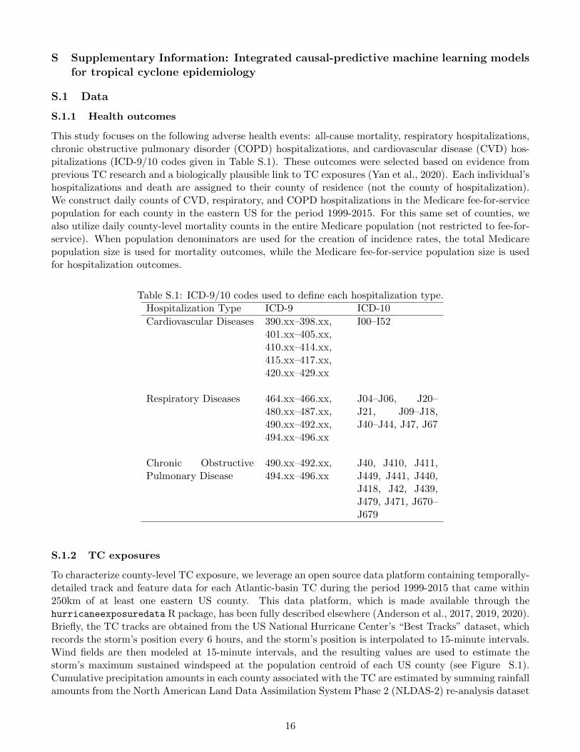
S Supplementary Information: Integrated causal-predictive machine learning modelsfor tropical cyclone epidemiology
S.1 Data
S.1.1 Health outcomes
This study focuses on the following adverse health events: all-cause mortality, respiratory hospitalizations,chronic obstructive pulmonary disorder (COPD) hospitalizations, and cardiovascular disease (CVD) hos-pitalizations (ICD-9/10 codes given in Table S.1). These outcomes were selected based on evidence fromprevious TC research and a biologically plausible link to TC exposures (Yan et al., 2020). Each individual’shospitalizations and death are assigned to their county of residence (not the county of hospitalization).We construct daily counts of CVD, respiratory, and COPD hospitalizations in the Medicare fee-for-servicepopulation for each county in the eastern US for the period 1999-2015. For this same set of counties, wealso utilize daily county-level mortality counts in the entire Medicare population (not restricted to fee-for-service). When population denominators are used for the creation of incidence rates, the total Medicarepopulation size is used for mortality outcomes, while the Medicare fee-for-service population size is usedfor hospitalization outcomes.
Table S.1: ICD-9/10 codes used to define each hospitalization type.Hospitalization Type ICD-9 ICD-10
Cardiovascular Diseases 390.xx–398.xx,401.xx–405.xx,410.xx–414.xx,415.xx–417.xx,420.xx–429.xx
I00–I52
Respiratory Diseases 464.xx–466.xx,480.xx–487.xx,490.xx–492.xx,494.xx–496.xx
J04–J06, J20–J21, J09–J18,J40–J44, J47, J67
Chronic ObstructivePulmonary Disease
490.xx–492.xx,494.xx–496.xx
J40, J410, J411,J449, J441, J440,J418, J42, J439,J479, J471, J670–J679
S.1.2 TC exposures
To characterize county-level TC exposure, we leverage an open source data platform containing temporally-detailed track and feature data for each Atlantic-basin TC during the period 1999-2015 that came within250km of at least one eastern US county. This data platform, which is made available through thehurricaneexposuredata R package, has been fully described elsewhere (Anderson et al., 2017, 2019, 2020).Briefly, the TC tracks are obtained from the US National Hurricane Center’s “Best Tracks” dataset, whichrecords the storm’s position every 6 hours, and the storm’s position is interpolated to 15-minute intervals.Wind fields are then modeled at 15-minute intervals, and the resulting values are used to estimate thestorm’s maximum sustained windspeed at the population centroid of each US county (see Figure S.1).Cumulative precipitation amounts in each county associated with the TC are estimated by summing rainfallamounts from the North American Land Data Assimilation System Phase 2 (NLDAS-2) re-analysis dataset
16

(Rui and Mocko, 2014) over a 4-day window beginning two days prior to the storm’s closest approach to thecounty (these precipitation data are currently available only for years 1999-2011). The county-level windand precipitation exposure metrics have undergone validation for use in epidemiologic studies (Andersonet al., 2020).
While the continuous windspeed and rainfall metrics are employed in the predictive component of themodel, for the causal inference component we must define a binary metric of TC exposure, which we referto as “treatment” for consistency with the causal inference literature. Counties exposed to the TC arereferred to as treated counties and those not exposed as control counties. Because previous epidemiologicresearch has suggested that TC windspeed is the feature most associated with acute health impacts (Yanet al., 2020), we use a maximum sustained windspeed threshold to classify counties as treated or control.Moreover, because TC windfields are large and relatively homogeneous over small areas, their use to defineTC exposure reduces within-county variation and the potential for exposure misclassification. We classifya county as treated for a given storm if it experienced sustained gale-force or higher sustained wind speeds(≥ 17.4 meters/second); otherwise, the county is classified as a control (Yan et al., 2020). This thresholdis consistent with the outer limit wind threshold used in the US National Hurricane Center’s wind radiiproduct for characterizing tropical cyclone size.
Figure S.1: Illustration of TC track and wind exposure measure for Hurricane Ike, 2008.
S.1.3 Exposure and health data linkage
Our analytic approach requires defining a study period for each TC, composed of a substantial time spanprior to the storm (used to establish baseline trends in health outcomes in treated and control counties) aswell as the period during and immediately after the storm (to estimate acute storm effects). For each TC,we define its study period as beginning 129 days prior to the TC’s first US approach and ending 11 daysafter. The TC’s first approach is the earliest date that the TC makes its closest approach to an exposedUS county/counties, which can be obtained from the hurricaneexposuredata package (Anderson et al.,2020). In practice, the approximately 18 weeks of outcome data prior to the TC exposure for each countyis aggregated into nine two-week counts of the outcome. Two-week cumulative counts are used because
17

narrower time intervals leads to small counts and instability in time series for many counties. We choose toemploy nine of these two-week counts because (1) this provides enough time points to reveal relationshipsin baseline trends in the health outcomes in treated vs. control counties while (2) the time series covers alimited enough period that relationships between the time trends in treated and control counties would beexpected to remain stable. The use of longer time series may introduce unnecessary noise into the modelsby capturing irrelevant long-term changes in relationships in baseline health across counties.
After designating each county in the study as treated or control for each TC as described above, weselect a set of analytic treated and control counties for a given TC as follows. Any county (treated orcontrol) is automatically excluded from the analytic set for a given TC if it has Medicare fee-for-servicepopulation size less than 100, or if it experiences 5 or fewer of any of the health events under studyduring the TC study period. Further, among the control counties, we select as analytic controls only thosethat fall within 150 miles of at least one treated county (distance computed between county centroids).Hereafter, when we reference the treated/control counties for a given TC, we are referring to the analytictreated/controls as defined here. We exclude TCs from the analysis if they have no valid treated counties,total sample size (treated + control counties) less than 20, or less than 5 control counties.
For each TC and each health outcome, we create a matrix of panel data, and these are central to thecausal inference component of our model. The panel data matrix is composed of rows corresponding toeach county in the analytic set for the given TC. Each row contains a time series of counts of the outcome inthat county, for each two-week interval during the TC study period. This results in 10 two-week intervals,i.e., 10 columns in the panel data matrix. We then define each time period for each county as a controlperiod or treatment period. For the control counties, all time periods represented in the panel data matrixare control periods. For treated counties, we consider the final two-week period, beginning 2 days beforeand ending 11 days after the TC’s first approach, to be the treatment period.
S.1.4 County and storm-specific features
Our predictive model will be used to capture the association between a TC’s health impacts and the TC’smeteorological features and the socioeconomic and demographic characteristics of the affected communities.To this end, for the predictive component of our model, we utilize the following TC features, which aredescribed in more detail by Anderson et al. (2020), for each TC-county pair (abbreviated variable name inparentheses): modeled maximum sustained wind speed at the population centroid of the county during theTC (vmax sust), duration of sustained wind speeds above 20 m/s at the population centroid of the countyduring the TC (sust dur), year the TC occurred (year), and total number of TC exposures experiencedby the county during 1999-2015 (exposure), which is a proxy for TC exposure propensity. For years 1999-2011, cumulative precipitation (precip) over a 4-day window, beginning two days prior to the TC’s closestapproach, is also available from the hurricaneexposuredata package. Because TC precipitation data arenot available for our full study period, we use it only for sensitivity analyses for the predictive models.
We also consider the following spatial, demographic, and socioeconomic features of the county: percentof residents in poverty (poverty), percent of residents self-identifying as White (white pct), percent of homesthat are owner-occupied (owner occupied), percent of residents age 65+ (age pct 65 plus), populationdensity (population density), median house value (median house value), percent of residents without ahigh school degree (no grad), a binary indicator of whether the county is located along the coastline (cc1),and the state the county is located in (state). These variables are extracted from US Census Bureauproducts. In particular we rely on the decennial census and American Community Survey (ACS). We alignthe demographic and socioeconomic features for each TC-county pair with the year of TC exposure. Foryears when census or ACS values are available, we use them directly, and in years not covered by the ACSor decennial census, we rely on interpolated values.
18
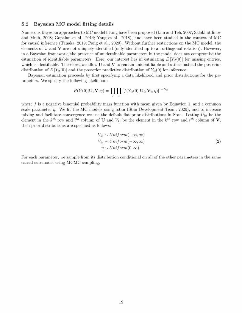
S.2 Bayesian MC model fitting details
Numerous Bayesian approaches to MC model fitting have been proposed (Lim and Teh, 2007; Salakhutdinovand Mnih, 2008; Gopalan et al., 2014; Yang et al., 2018), and have been studied in the context of MCfor causal inference (Tanaka, 2019; Pang et al., 2020). Without further restrictions on the MC model, theelements of U and V are not uniquely identified (only identified up to an orthogonal rotation). However,in a Bayesian framework, the presence of unidentifiable parameters in the model does not compromise theestimation of identifiable parameters. Here, our interest lies in estimating E [Yit(0)] for missing entries,which is identifiable. Therefore, we allow U and V to remain unidentifiable and utilize instead the posteriordistribution of E [Yit(0)] and the posterior predictive distribution of Yit(0) for inference.
Bayesian estimation proceeds by first specifying a data likelihood and prior distributions for the pa-rameters. We specify the following likelihood:
P (Y (0)|U,V, η) =∏i
∏t
[f(Yit(0)|Ui,Vt, η)]1−Dit
where f is a negative binomial probability mass function with mean given by Equation 1, and a commonscale parameter η. We fit the MC models using rstan (Stan Development Team, 2020), and to increasemixing and facilitate convergence we use the default flat prior distributions in Stan. Letting Uki be theelement in the kth row and ith column of U and Vkt be the element in the kth row and tth column of V,then prior distributions are specified as follows:
Uki ∼ Uniform(−∞,∞)
Vkt ∼ Uniform(−∞,∞)
η ∼ Uniform(0,∞)
(2)
For each parameter, we sample from its distribution conditional on all of the other parameters in the samecausal sub-model using MCMC sampling.
19

S.3 Causal identifying assumptions
In the most general setting, the potential outcomes for our panel data would be defined as Y(d), a matrixcontaining all outcomes when treatment statuses for all units at all time points are given by the matrix d.In this general case, each unit’s potential outcomes depend on the treatment status of all units at all timepoints. In order to define the potential outcomes more concisely as we have in the paper, we invoke theclassic Stable Unit Treatment Value Assumption used in causal inference (Rubin, 1980), which states that1) there is only one version of treatment and that 2) one unit’s outcome is unaffected by the treatmentstatus of other units. If SUTVA is met, then we can define a unit’s potential outcomes at time t as Yit(di),where di is a binary T -length vector of the treatment status of unit i at times 1, ..., T .
In order to define a unit’s potential outcomes at time t as a function of only its treatment statusat time t, as we have done in the main text, we are implicitly making the standard assumption thatfuture treatment cannot impact past outcomes and making an additional assumption about the impact oftreatment histories. That is, we assume that a unit’s full historic treatment status vector is a deterministicfunction of the unit’s time of initial treatment adoption, so a unit’s potential outcomes can be expressedas functions of only the unit’s time of initial treatment adoption, rather than functions of its full historictreatment status vector. The panel data construction described in the main text is designed to satisfy thisassumption, by requiring that treated units initiate treatment at some time T0 > 1 and remain treatedthrough time T . In general, we can allow for varying initiation times by unit, denoted by T0i. In this setting,the treatment assignment vector di is determined entirely by treatment initiation time T0i, such that we canwrite the observed treatment vector as di(T0i). Under this assumption, we can write Yit(di = 0) = Yit(0),since treatment history is fully determined for a unit that has not yet initiated treatment. For treatedunits, because Yit(di(T0i)) is observed when t ≥ T0i, it can be treated as a known quantity and simplifiedto Yit(1). Then for i ∈W, t ≥ T0i we can define the IEE as θi =
∑t≥T0
[Yit(1)− Yit(0)].We posit 4 additional assumptions that are needed to identify the causal effects of a TC using the
proposed matrix completion approach.
Assumption 1: Causal consistency. This assumption states that the observed outcome is equal to thepotential outcome under the observed treatment level, i.e.,
Yit(d) = Yit if Dit = d
Assumption 2: Latent ignorability. Let Yi(0) be the vector of outcomes under control for unit i andYi(0)obs be the observed elements of Yi(0). This assumption states that conditional on observed covariatesused in the causal model, Zi (if any are used), the latent variables, U′iV, and the observed outcomesunder control, Yi(0)obs, the treatment assignment is independent of the potential outcomes under control.This assumption is analogous to, but weaker than, the classic ignorability assumption required for causalinference, because it allows for unmeasured confounding to be captured either by observed variables, or bythe time-varying latent variable. Formally, this assumption is written as
T0i ⊥⊥ Yi(0) | Yi(0)obs,Zi,UTi V
Assumption 3: Approximation of unobservables. This assumption states that the matrix of unobservedfeatures impacting the outcomes over time can be approximated through a low-rank matrix factorization.Equivalently, this requires that the unobserved time-varying confounders can be captured by a smallnumber of latent factors, K, defined by the matrix factorization. This assumption is analogous to theassumption of correct model specification in standard regression models, but adapted to the context oflatent variable models. Formally, this assumption requires that, for each unit, there is a latent (possiblytime-varying) confounder of the treatment effect, Wi, that can be approximated by a low-rank matrix
20

factorization Wi = UTi V.
Assumption 4: Conditional exchangeability. Conditional on any observed covariates Z, and latentvariable W, elements of Y(0) are exchangeable. This assumption is needed in order to define the posteriorpredictive distribution used to estimate the missing values in Y(0).
Under these assumptions, Pang et al. (2020) show that the causal effects are identified by Bayesianmatrix completion models.
21
S.4 Bayesian modularization
Our modularized model can also be viewed as a complex Bayesian multiple imputation procedure. Causalinference in the potential outcomes framework is often treated as a missing data problem, i.e., the coun-terfactual outcomes are considered missing data that needs to be imputed. In our case, the TC-specificcausal inference models are used to impute counterfactual outcomes, and the resulting treatment effectsfrom all the TCs are passed into the predictive model. Although the causal and predictive models suggestincompatible distributions for the missing counterfactual outcomes, the use of incompatible imputationand analysis models has been well-studied. This approach, often referred to as a fully conditional modelspecification, incompatible Markov Chain Monte Carlo (MCMC), or multiple imputation with incongenialsources of input, has been shown to often perform better than fully Bayesian data augmentation withcomplex models (Meng, 1994; Rubin, 2003; Schafer, 2003; Van Buuren et al., 2006; Van Buuren, 2007; Kuoand Wang, 2018).
We introduce our modularization approach using this missing data perspective. Our goal is to illustratethe principles used to modularize the model by providing general forms of the modularized full conditionaldistributions of all parameters. For a given TC s, denote by Ys(0) the full set of potential outcomesunder control, composed of both the observed values Y obs
s (0) and the missing values Y miss (0). The causal
component of the model aims to estimate the Y miss (0). Denote the TC-specific causal parameters by φs
and denote the treatment indicators for each unit/time collectively as Ds (note that from the missing dataperspective, the treatment indicators can be viewed as missingness indicators). We assume throughoutthis section that Ys(1), the (observed) potential outcomes under treatment for the treated units at post-treatment times, are fixed and known quantities. Then the IEEs, θs, are assumed to be a deterministicfunction of the Y mis
s (0). In the predictive component of the model, let X denote the predictors and βdenote the predictive model parameters. (We again focus on a single outcome-specific model.)
Then the posterior distribution of the parameters and missing data can be expressed as
P
({Y miss (0)
}S
s=1, {φs}Ss=1 , β |
{Y obss (0)
}S
s=1, {Ds}Ss=1 , X
)Traditional Bayesian MCMC sampling algorithms successively sample from the full conditional poste-
rior distribution of each of the unknown parameters. For the missing data, we obtain the following fullconditional distribution
P
({Y miss (0)
}S
s=1|{Y obss (0)
}S
s=1, {Ds}Ss=1 , X, {φs}Ss=1 , β
)∝P
({Y obss (0)
}S
s=1,{Y miss (0)
}S
s=1, {Ds}Ss=1 , X | {φs}Ss=1 , β
)=P
({Ds}Ss=1 |
{Y obss (0)
}S
s=1,{Y miss (0)
}S
s=1, X, {φs}Ss=1 , β
)×
P
({Y obss (0)
}S
s=1, |
{Y miss (0)
}S
s=1, X, {φs}Ss=1 , β
)×
P
({Y miss (0)
}S
s=1| X, {φs}Ss=1 , β
)×
P(X | {φs}Ss=1 , β
)Then if we assume that {
Ds, Ymisss (0), Y obs
s (0)}⊥⊥{Ds′ , Y
misss′ (0), Y obs
s′ (0)}
s′ 6=s| φs
we obtain
S∏s=1
P(Ds | Y obs
s (0), Y miss (0), X, φs, β
)P(Y obss (0) | Y mis
s (0), X, φs, β)P(Y miss (0) | X,φs, β
)P(X | {φs}Ss=1 , β
)Then assuming the causal identifying assumptions hold, we have unconfoundedness conditional on the
causal model parameters, so that P(Ds | Y obs
s (0), Y miss (0), X, φs, β
)= P
(Ds | Y obs
s (0), X, φs, β), which
does not depend on Y miss (0) and thus drops out. P
(X | {φs}Ss=1 , β
)also does not depend on Y mis
s (0)
22
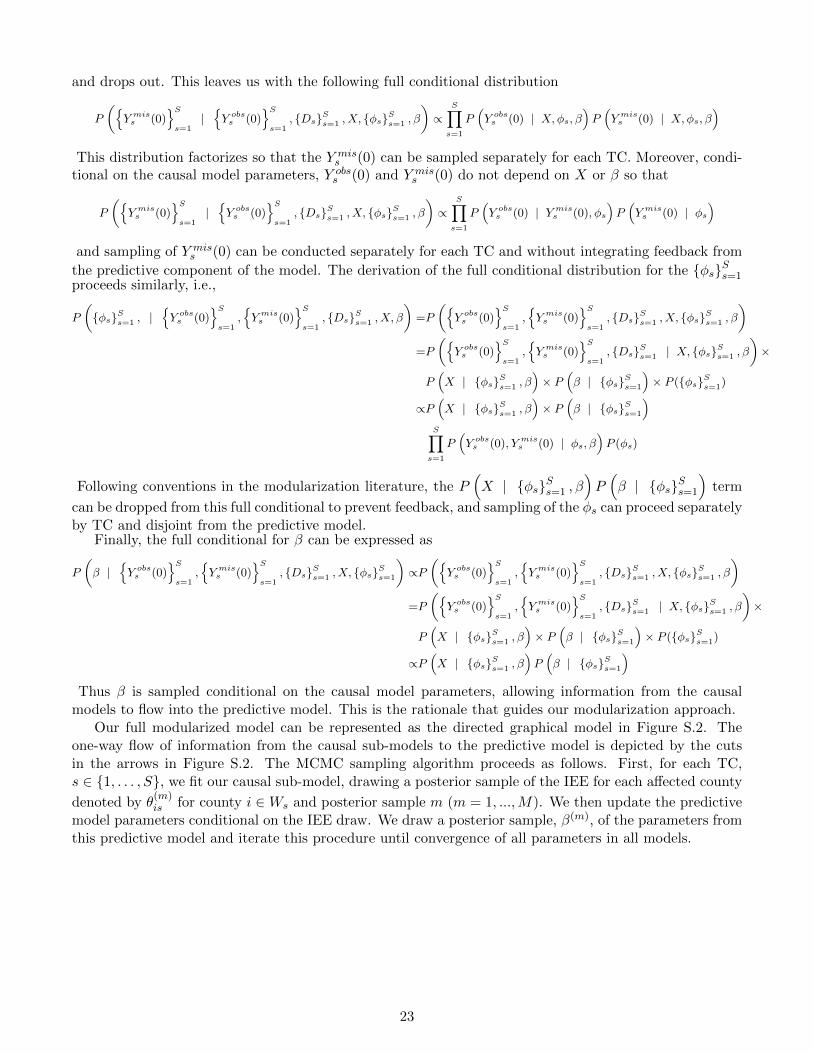
and drops out. This leaves us with the following full conditional distribution
P
({Y miss (0)
}S
s=1|{Y obss (0)
}S
s=1, {Ds}Ss=1 , X, {φs}Ss=1 , β
)∝
S∏s=1
P(Y obss (0) | X,φs, β
)P(Y miss (0) | X,φs, β
)This distribution factorizes so that the Y mis
s (0) can be sampled separately for each TC. Moreover, condi-tional on the causal model parameters, Y obs
s (0) and Y miss (0) do not depend on X or β so that
P
({Y miss (0)
}S
s=1|{Y obss (0)
}S
s=1, {Ds}Ss=1 , X, {φs}Ss=1 , β
)∝
S∏s=1
P(Y obss (0) | Y mis
s (0), φs
)P(Y miss (0) | φs
)and sampling of Y mis
s (0) can be conducted separately for each TC and without integrating feedback from
the predictive component of the model. The derivation of the full conditional distribution for the {φs}Ss=1proceeds similarly, i.e.,
P
({φs}Ss=1 , |
{Y obss (0)
}S
s=1,{Y miss (0)
}S
s=1, {Ds}Ss=1 , X, β
)=P
({Y obss (0)
}S
s=1,{Y miss (0)
}S
s=1, {Ds}Ss=1 , X, {φs}Ss=1 , β
)=P
({Y obss (0)
}S
s=1,{Y miss (0)
}S
s=1, {Ds}Ss=1 | X, {φs}Ss=1 , β
)×
P(X | {φs}Ss=1 , β
)× P
(β | {φs}Ss=1
)× P ({φs}Ss=1)
∝P(X | {φs}Ss=1 , β
)× P
(β | {φs}Ss=1
)S∏
s=1
P(Y obss (0), Y mis
s (0) | φs, β)P (φs)
Following conventions in the modularization literature, the P(X | {φs}Ss=1 , β
)P(β | {φs}Ss=1
)term
can be dropped from this full conditional to prevent feedback, and sampling of the φs can proceed separatelyby TC and disjoint from the predictive model.
Finally, the full conditional for β can be expressed as
P
(β |
{Y obss (0)
}S
s=1,{Y miss (0)
}S
s=1, {Ds}Ss=1 , X, {φs}Ss=1
)∝P
({Y obss (0)
}S
s=1,{Y miss (0)
}S
s=1, {Ds}Ss=1 , X, {φs}Ss=1 , β
)=P
({Y obss (0)
}S
s=1,{Y miss (0)
}S
s=1, {Ds}Ss=1 | X, {φs}Ss=1 , β
)×
P(X | {φs}Ss=1 , β
)× P
(β | {φs}Ss=1
)× P ({φs}Ss=1)
∝P(X | {φs}Ss=1 , β
)P(β | {φs}Ss=1
)Thus β is sampled conditional on the causal model parameters, allowing information from the causal
models to flow into the predictive model. This is the rationale that guides our modularization approach.Our full modularized model can be represented as the directed graphical model in Figure S.2. The
one-way flow of information from the causal sub-models to the predictive model is depicted by the cutsin the arrows in Figure S.2. The MCMC sampling algorithm proceeds as follows. First, for each TC,s ∈ {1, . . . , S}, we fit our causal sub-model, drawing a posterior sample of the IEE for each affected county
denoted by θ(m)is for county i ∈Ws and posterior sample m (m = 1, ...,M). We then update the predictive
model parameters conditional on the IEE draw. We draw a posterior sample, β(m), of the parameters fromthis predictive model and iterate this procedure until convergence of all parameters in all models.
23

!"($)
&
'
(
)"*+!,($)
!-($)
*.
*/
),
)-
⋮ ⋮Figure S.2: DAG for Bayesian modularization
24

S.5 Population displacement
The zipcode/county of residence recorded in Medicare claims data for each recipient is updated yearly andrepresents their place of residence at either the end of the specified year or early the following year (timingchanges slightly year-to-year). This implies that, if a person moves from county A to county B duringa given year, all their hospitalizations for that year will be assigned to county B. Because the Atlantichurricane season occurs primarily in the latter half of the year (June-November), use of the county ofresidence at year’s end for exposure classification and population denominator construction is generallyappropriate.
Yet, for a few severe storms that resulted in substantial long-term population displacement, suchas Hurricane Katrina (Deryugina and Molitor, 2018), some degree of exposure misclassification is likely.However, we would expect that the impact of any such exposure misclassification would be to bias IEEstowards the null. Consider a scenario in which county A is exposed to a TC and county B is a control forthat TC. Then, if a person living in county A at the time of exposure is hospitalized due to the TC, butis displaced to county B before the end of the year, their TC-attributable hospitalizations will be assignedto control county B. The resulting increase in adverse event rates in control counties should lead to anupward bias in the estimated Yit(0), t ≥ T0 and a corresponding downward bias in the IEE for the exposedcounties. In spite of this potential for underestimated IEEs, we estimate large adverse health impacts forHurricane Katrina. For most other TCs assessed by our study, we would expect that TC-related long-term displacement rates are low, based on previous work that found that, even for unusually strong TCs(Category 3 or greater at landfall), outward migration increases on average by only 6.85% in the yearfollowing the storms (Ouattara and Strobl, 2014).
25

S.6 Selection of K
We wish to select a K value that preserves approximately 70% of the variance in the panel data matrix forall TCs and all outcomes. 70% is chosen because it represents a compromise between retaining variabilitynecessary for accurate predictions, while not overfitting to the data. To explore the choice of K that bestsatisfies this criterion, we conduct exploratory principal component analyses (PCA) on the panel datamatrices. Specifically, we remove the final column of the panel data matrix for each TC and outcome(because it contains missing values which are not permitted in PCA), and we implement PCA on eachresulting matrix. The scree plots showing the percent of variance explained by each prinicipal component(for each panel data matrix) are shown in Figure S.3. On average across TCs, the first four principalcomponents explain 63% of the variance in mortality, 73% in respiratory hospitalizations, 70% in COPDhospitalizations, and 74% in CVD hospitalizations. Thus K = 4 appears to be a reasonable choice topreserve around 70% of the variability in the panel data matrices. Moreover, as demonstrated by Figure S.3,each principal component beyond the fourth generally explains less than 10% of the variance in the paneldata.
●
●
●
● ●
●●
●
●
●●
●●
●●
●●
●
●
●●
●● ●
●
●
●
●
●●
●
●
●●
●●
●
●
●● ●
●
● ●●
●
●
●
●
●●
●●
●
●
●
●●
●●
●●
●
●
●
●
●
●
●●
●●
●
●
● ●
●
●
●
●●
●
●
●●
●●
●● ●
●
●
●
●
●
● ●
●
●
●
●
●
●●
●
●●
●
●
●
●
●
●
●
●
●
●
●
●
●●
●●
● ●●
●
●
●●
●●
●● ●
●
●
●●
● ●
●
●
●
●
●
●
●●
●
●●
●
●
●
●●
●
●
●
●●
●
●
● ●●
●
●●
●
●
●●
●●
●●
●
●
●
●● ●
●
●
●●
●
●
●
●
●
●
● ●● ●
●
●
●
●
●
●
●
●
●
●
●
●
●
●
●●
●
●
●
●
●
●
●
● ●●
●
●
●●
●
●●
●
●
●
●
●
●●
●
●
●●
●
●
●●
●
●
●
●
●
●
●
●
●
●
●
●
● ●
●
●
●
●
●
●
●
●
● ●
●
●
●
●● ●
●●
●
●
●
●
●
●
●
●
● ●
●
●●
●
●
● ●●
●
●
●
●
●
●
●
●●
●
●
●
●● ●
● ●
●
●
●
●
●
●
●
●
●
●
●
●
●
●
●
●
●
● ●
●
●
●●
●
●●
●●
●
●
●●
●●
●●
● ●
●
●
●●
●
●●
● ●
●
●●
●
●
●
●
●●
●
●●
●
●●
●●
●
●
●
●
●●
●●
●
●
●●
●
●●
●
●
●●
●
●
●
●
●●
●●
●
●
●
●
●●
●●
●
●
●
●
●
●●
●
● ●
●
●
●●
● ●
●
●●
●
●
●
●●
●
● ●
● ●
●
●
●●
●
●
●●
●
●
●
●
●
●●
●●
●
●
●
●
● ●
●
●●
●
●
●
●
●●
●
● ●
●
0.0
0.1
0.2
0.3
0.4
1 2 3 4 5 6 7 8 9Component
% V
aria
nce
Exp
lain
ed
A
●
●
● ●
●● ●
●●
●
●
●
●● ●
●●
●
●
● ●
● ●●
● ● ●
●
●
●●
●
● ●●
●
●
●●
●
● ● ●● ●
●
●
●
● ●● ●
●●
●
●●
● ●●
●●
●
●
●
●● ●
●●
● ●
●
●
●
●●
●●
●●
●
●
●●
●●
●● ●
●
●
●●
● ●● ●
●
●
●
●
● ●
●
● ●●
●
●
●
●
● ●●
●
●
●
●
●
●●
●● ●
●
●
●
●
● ●●
● ●
●
●
●
●●
●
●
●●
●
●
●
●
●●
●●
●●
●
●
●●
●● ●
● ●
●
●● ●
●● ●
●●
●
●
●●
●
● ●
● ●
●
●
●●
● ●● ●
●
●
● ● ●● ●
● ●●
●
●
●
●
●●
●
●●
●
●
●●
●
● ●● ●
●
●●
●● ●
●● ●
●
●
●
●● ●
●●
●
●
●
●
●
●●
●●
●
●
●
●●
●●
●●
●
●
●
● ●
●
● ●●
●
●
●
●
●
●
●
●● ●
●
● ●●
●● ● ●
●
●
● ●
●
●●
● ●●
●
●
●●
●
● ●
● ●
●
●
●
●
●
● ● ● ●
●
●
●●
●● ●
●●
●
●
●
●
●●
●
●●
●
●
●●
●●
●
● ●
●
● ●● ●
●● ●
●
●
● ●
●●
●●
●
●
●
●
●
● ●●
●● ●
●
● ●
●●
●●
● ●
●
● ● ●●
●●
● ●
●
●
●●
●● ●
●●
●
● ●●
●● ● ● ●
●
●
●●
●
● ●● ●
●
● ●
●●
●
● ●●
●
●
●
●● ●
● ●
●
●
●
●● ● ●
● ●
●
●
●
●● ●
●
●
● ●
●
●●
●●
●● ●
●
●
●●
●●
● ●●
●
●
●
●
●
●●
● ●●
●
●
●●
●●
●● ●0.0
0.2
0.4
0.6
1 2 3 4 5 6 7 8 9Component
% V
aria
nce
Exp
lain
ed
B
●
●● ●
●
● ●●
●
●
●
●●
●
●●
●
●
●
●●
●
● ●● ●
●
●
●●
●
●● ●
●●
●
●
●●
●●
● ●●
●
●●
●
●●
●● ●
●
●●
●●
●● ●
●
●
●
●●
●
●
● ●
●
●
●
●
●
●●
● ● ●
●
●●
●
●
●●
●●
●
●
●
●●
● ●● ●
●
●
●
●
● ●
●●
●
●
●
●
●
●●
● ●
●
●
●
●
●●
●● ●
●
●
●
●●
●
●●
●
●
●
●●
●
●
● ●
●●
●
●
●●
●
● ●
●●
●
●
●
●
● ●●
● ●
●
● ●
● ●●
●
●●
●
●
●
●●
●
●
●
●
●
●
●●
●●
●●
●
●
● ●
● ●
● ●
●●
●
●
●
●●
●
●
●●
●
●
●●
●●
●●
●
●
●
● ●
● ●● ●
●
●
●
●
●●
● ● ●
●
●
●
●
●
●
● ●
●●
●
●
●
●
●●
●●
●
●
●
●
●●
●●
●
●
●
●
●●
●
●
● ●●
●
●●
● ●●
●●
●
●
●
●●
●
●●
●●
●
●
● ●●
●
●● ●
●
●
●
● ●
●●
● ●
●
●
●
●●
●● ●
●
●
●
●
●●
●
●●
●
●
●
●●
● ●●
●●
●
●
●●
● ●●
●●
●
●
●●
●● ●
●
●
●
●
●
● ●
●●
●●
●
●
●●
●
●●
● ●
●
●●
● ●● ●
● ●
●
●●
●●
●●
●
●
●
●●
● ●
●● ●
●
●
●●
●●
●●
● ●
●
●
●
●
● ●●
●●
●
●
● ●
● ●●
●●
●
●
●
● ●●
●●
●
●
●
●●
●● ●
●●
●
●
●●
●●
● ●●
●
●
●●
●
● ●●
●
●
●
●
●●
●●
● ●
●
●
●
●
●●
● ●●0.0
0.2
0.4
0.6
1 2 3 4 5 6 7 8 9Component
% V
aria
nce
Exp
lain
ed
C
●
●
●
●
●● ●
● ●
●
●
●● ●
●
●
● ●
●
●● ●
●
● ● ●●
●
●
●
●●
●● ●
●
●
●
●●
●● ●
●
●
●
●
●
● ●●
●●
●
●
●●
●●
●●
● ●
●
●
●
●
●● ●
●
●
●
●
●
●●
●
● ● ●
●
●
●
●
● ●
●
● ●
●
●
●
● ●
●
● ●●
●
●
●
●
●
●●
● ●
●
●●
●●
● ●
●●
●
●
●
●● ●
● ●
●
●
●
●
●
●●
● ●●
●
●
●
●●
●●
●●
●
●
●●
●● ●
●●
●
●● ●
●
●●
● ●
●
●
●
●●
●●
● ●
●
●
●
●
●
●●
●
●
●
●
●●
●
●●
●●
●
●
●● ●
●●
●●
●
●
●●
●
●
●●
●
●
●
●
●● ●
●●
●
●
●
●
●● ●
● ●●
●
●●
●● ●
● ● ●
●
●
●
●
●●
●
● ●
●
●
●●
● ●●
●●
●
●
● ●●
●●
● ●
●
●
●
●
●●
●● ●
●
●● ●
●
● ●●
●
●
●
●●
● ●●
●●
●
●●
●●
● ● ●●
●
●
●●
●
● ● ● ●
●
●
● ●
● ●●
● ●
●
●
●
●
●
●●
●●
●
●●
●●
●● ●
●
●
●●
● ● ●
●● ●
●
●
●●
●● ●
●●
●
●
●●
●● ●
● ●
●
●
●●
●●
● ●●
●
●●
●● ●
● ● ●
●
●●
●
●●
●● ●
●
●●
●●
●● ● ●
●
●
●
●●
● ●●
●
●
●●
●● ●
● ●●
●
●●
● ●
● ●● ●
●
●● ●
●●
● ●●
●
●
●●
●●
● ●
●
●
●
●● ●
● ● ●●
●
●●
●●
●● ●
●
●
●
●●
●
●
●
●●
●
●
●
●
●
● ● ● ●
0.0
0.2
0.4
0.6
1 2 3 4 5 6 7 8 9Component
% V
aria
nce
Exp
lain
ed
D
Figure S.3: Scree plots for PCA fit to the panel data matrix for each TC for mortality (A), respiratoryhospitalizations (B), COPD hospitalizations (C), and CVD hospitalizations (D).
26

S.7 Predictive model selection
Candidate predictive models are Bayesian additive regression trees (Chipman et al., 2010) (BART) andnumerous variants of a linear regression model. In the regression models, we always include a restrictedcubic spline on year to allow for flexible time trends in health effects of TCs. We consider regression modelswith (1) all additional predictors included as linear terms, (2) a restricted cubic spline on TC maximumsustained windspeed and all additional predictors included as linear terms, and (3) interactions betweenall predictors and a binary indicator of hurricane-speed winds (sustained windspeeds > 33m/s). We testeach predictive model candidate both with and without state included as a predictor.
To evaluate and compare predictive models, we fit them by plugging in the county-level excess rate pointestimates as the outcomes (without passing their full posterior distributions into the predictive model).Using five-fold cross-validation, we compare out-of-sample predictive performance of these models. Rootmean square error for each model is given in Table S.2. For most outcomes, we find similar predictiveperformance across models. Overall, we find the most consistently strong performance for the regressionmodels with splines on windspeed, excluding state. Thus, for the primary predictive sub-model, we selectthe Bayesian linear model with a spline on windspeed, excluding state as a predictor. For interpretability,we also provide results from a linear regression model without the windspeed spline.
Table S.2: Root mean square error from 5-fold cross-validation for each considered predictive model.Mortality Resp COPD CVD
Linear with state 90.15 64.24 41.82 96.99Linear without state 89.96 64.34 42.08 95.84
Spline with state 89.92 64.15 41.88 96.99Spline without state 89.59 64.25 42.14 95.83
Linear, hurricane stratified 92.15 64.57 42.41 96.04Spline, hurricane stratified 92.17 64.57 42.45 96.05
BART with state 90.85 64.28 41.53 95.85BART without state 101.36 64.26 41.97 96.07
27
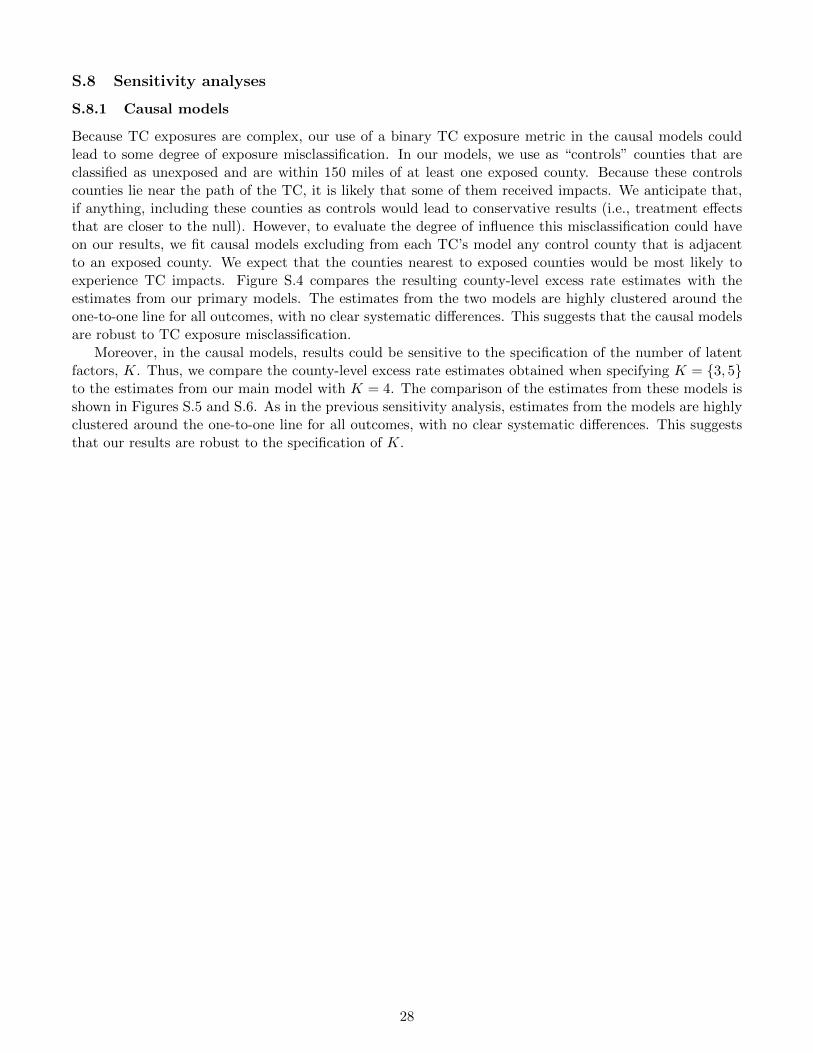
S.8 Sensitivity analyses
S.8.1 Causal models
Because TC exposures are complex, our use of a binary TC exposure metric in the causal models couldlead to some degree of exposure misclassification. In our models, we use as “controls” counties that areclassified as unexposed and are within 150 miles of at least one exposed county. Because these controlscounties lie near the path of the TC, it is likely that some of them received impacts. We anticipate that,if anything, including these counties as controls would lead to conservative results (i.e., treatment effectsthat are closer to the null). However, to evaluate the degree of influence this misclassification could haveon our results, we fit causal models excluding from each TC’s model any control county that is adjacentto an exposed county. We expect that the counties nearest to exposed counties would be most likely toexperience TC impacts. Figure S.4 compares the resulting county-level excess rate estimates with theestimates from our primary models. The estimates from the two models are highly clustered around theone-to-one line for all outcomes, with no clear systematic differences. This suggests that the causal modelsare robust to TC exposure misclassification.
Moreover, in the causal models, results could be sensitive to the specification of the number of latentfactors, K. Thus, we compare the county-level excess rate estimates obtained when specifying K = {3, 5}to the estimates from our main model with K = 4. The comparison of the estimates from these models isshown in Figures S.5 and S.6. As in the previous sensitivity analysis, estimates from the models are highlyclustered around the one-to-one line for all outcomes, with no clear systematic differences. This suggeststhat our results are robust to the specification of K.
28

●●●
●
●
●
●●
●
●
●●●●
●●●●
●●●●●
●●●●●
●●●●●●●●●●
●●●●●●●
●●●●●
●●
●●
●
●
●●●●●
● ●●●
●
●
●●●●●
●
●●●●●●●●●
●
●
●●●
●
●●●●●●●●●
●●●
●
●●
●●●●●●●●●●●●
●●●●●●●
●●●●●●●●●●
●●●●●
●
●●●●●●●●●●●
●●●
●●●
●●
●●●
●●●●●●
●●●●●●●
●●●
●●●●●●●●●●
●●●●●
●●●●●
●
●●●●
●
●●
●●●
●●
●●●●●●●
●●●●
●●●●●●●
●● ●●
●●
●●●●●●●●●
●
●●
●●●
●●●
●●
●●●●
●●●
●●●●
●●●●
●
●
●●●
●
●●
●●●●●●
●●●
●●●
●●
●●
●
●●●●
●
●●●●●●●
●●
●
●●●
●
●●●●●●●
●
●●●●
●
●●●●●●●●●●
●●●
●●●●●●●●
●●●●●●●●●●●●●●●
● ●
●●●
●●
●●●●●●
●
●●●●●
●●
●●
●●
●
●
●
●●●
●●
●
●●
●●●●
●●
●●
●●●●●●●●
●
●●●
●●
●
●
●●
●●●
●●
●
●●●●●
●●●●●
●
●●
●●
●
●●●
●
●●
●●●
●●
●
●●
●●●●
●●
●
●●●●
●
●●●●
●●●
●●●●
●●●●●
● ●●●●●
●
●●●●●
●●
●
●●●●
●●
●●●●●●●●●
●
●●●●●●●●●●●●●
●●●
●
●●●●
●
●●●●●●
●●●
●
●
●
●●
●●
●●●●●●
●
●●
●
●●●
●●●
●
●●
●●●●
●
●●
●●●●●●●●●●
●●●●●●●
●●
●●●●●●●●●●●
●●
●
●
●●●●
●●
●
●●●●●
●
●
●●●●●●
●
●
●●●
●
●
●
●●
●●●●
●●●●
●●●●●
●●
●●
●
●●●
●●●
●●
●●●●●●
●
●
●●●●
●●
●●●●●●●●●
●●●
●●
●●
●●●●●●●●●●●
●●●●
●●
●●
●●●●●●●
●●●●●●●●●●●●●●●
●●●●
●
●●●
●●●●
●●
●
●
●●●●●●
●●●●●●●●
● ●●●
●●●●●●
●●●●●● ●●●
●
●● ●●
●
●●
●●●●●
●●●●●●●●●
●
●
●
●●
●●
●●
●●●●●●● ●●●
●●
●●●●●●●●
●●●●●●●
●
●●●●●
●
●●
●●●
●●
●●
●
●
●
●●●●●●
●●●
●●●●●●●●
●●●●●
●●
●●
●●●
●
●●●
●
●
●●●
●●●●
●●
●●●
●●●
●●●●●
●
●●●
●
●
●●●● ●●
●
●●
●
●●●●●●●
●●●●●●
●●●●
●●●●●
●●●●
●
●●
●
●●●●
●●●●●●●●●
●
●●●●
●●
●
● ●●●
●●●●
●●
●●●●●●●●●●
●●●●●●●●●●●●●●●●●●●●●●●●●●●●●●●
●●
●●●●●
●●●●●●
●●
●●●
●●●
●●●●
●
●
●
●●●●●●●
●
●●●
●●●
●
●
●●
●●
●●
●
●●
●●
●
●
●●● ●●
●●
●●●●●
●●●
●●
●
●●●●●●
●
●
●●●
●● ●
●●● ●
●
●
●
●●●
●●●
●●●●●
●●
●●
●
●
●●
●●
●●
●
●●●●
●●
●●
●●●
●
●●
●
● ●●●
●●
●
●●●●●●
●
●
●
●
●●●●●● ●
●●
●●
●
●●●●●●
●●
●
●●●●●●
●● ●●
●●
●
●●●●●●●
●
●
●
●●●
●●●●●
●●●●
●●●●●●
●
● ●
●●
●
●●●●●●
●●●●●●●
●●
●●●●●●
●
●●●●●
●●●
●
●●●
●●
●●●●●
●●●
●●
●
●●●●
●
●●
●
●●●
●●●
●●
●
●
●●●● ●
●
●●●
●●●●●
●
●●●●●●●●●●
●
●
●●●
●●●●●
●●
●
●●●●
●●●●●
●
●●●●
●●●
●●●●●
●●
●●●●
●
●●●●●●●●●●●●
●
●●●●●
●●●●●
●●●●●●●●●●●●●●
●●
●●●●●●●●●●●●●●●●●●●●●●●●●●●●●●●●●●●●●●
●●●●●●●●●●●●●●●●
●●●●●●
●●●
●●●●●
●
●
●●●●
●
●
●●●
●●●●
● ●●●
●
●●
●●
●●●●●
●●●
●
●●●●
●●
●
●
●●●
●
●●
●●●●
●●●●●
●●
●●●
●●●
●●
●●
●
●●●●
●
●●
●
●●●●●●●
●●
●
●●
●●
●●●●●●●
●
●
●
●
●
●●●●
●
●●●●
●●
●
●
●●●●●●●●●●
●●
●
●●
●
●●
●
●●
●●●
●●
●●
●●●
●
●●
●●
●●●
●●
●●●
●●
●
●
●●●●●
●
●
●●●●●●●●
●●●●●●
●
●●●
●●
●
●
●●●●
●●●
●●●●●●●●●
●●●
●●
●
●●●
●●●●
●●
●●
●
●
●
●
●●●●●
●●●●
●
●
●●
●
●●
●
●
●
●●●
●
●●●● ●●
●●●●●
●
●●●
●●●●● ●
●●●●●●●●
●●
● ●●
●
●● ●●
●●
●
●
●●●
●
●
●
●●
●
●●
●●●●
●
●●●●●●●
●●
●
●
●
●●
●●●●●●
●●
●
●
●
●●●
●●●●
●
●●●
●
●
●
●●●
●●
●
●
●●
●
●●
●
●●●●●●●●●●●
●●●●●●
●●
●●
●●
●
●
●●●
●●● ●
●●●● ●
●●●●
●●●●
●●
●
●●●●●●
●●
●●
●
●●●●●●●
●
●●●●●●●●
●●
●●●●●●●
●● ●●●●●
●
●●●●●●
●●●●
●●
●●
●●
●●
●
●●●
●
●●●
●●
● ●●
●●
●●
●
●●
●
●●●●●●●
●●●●●●●●●
●●●
●●●●●
●●●●●●●●●●●●●●●●●●●
●●●●●
●
●●●●
●●●●●
●
●●●
●●●●●●
●●●●●
●●●●●●●
●●●●
●●●●●
●●●
●●●●●●●●●
●●●●●●●●
●●●●
●●●●●
●●●●●
●
●●●●●●●
●
●●●●0
1000
2000
0 1000 2000Main Model
Com
paris
on M
odel
MortalityA
●●●●●
●●●●● ●●●
●
●●●
●●●●●●●
●●●●●●●●●
●●
●●●●●
●●
●
●●
●
●
●●●
●●●
●●
●●
●●●
●●
●●
●
●●
●●
●●
●
●
●●●
●●●
●●
●
●●
●
●●●
●●●
●●●●●
●●●●
●
●●
●●
●
●●
●●
●●
●
●●●●●●●●●
●●●●
●●
●●
●
●●●
●
●●
●
●●●●●●
●●●
●●●
●
●●●
●●
●●●●●●●
●●●●●
●●●
● ●●●●
●●●●●●
●
●●
●
●●●●●●●●●
●
●
●
●●
●●
●
●●●
●
●
●●
●●●●●
●●
●●
●●●●●
●●●
●●●
●●●
●
●●●●●●●●●●
●
●
●●●●●●● ●●●●●●
●●
●●●●●
●●
●
●●
●
●
●
●
●●●
●●
●
●
●●●●●
●●
●●●
●
●
●●●●●●
●●●
●●●●
●●●●●●
●●
●●●●●●●
●●●
●●●●●●●●
●●
●●●
●●●●●●
●●
●
●●●●●●●●●●●●●●
●●●●●●
●●
●
●●●●
●●
●
●
●
● ●●●
●●
●●●
●
●●●
●●●
●
●●
●
●●
●●
●●●●
●
●●●●
●
●
●●
●
●●●●
● ●●●
●
●●●
●
●●●●
●●●●
●
●●●●
●
●
●
●
●●●
●●●
●
●
●
●
●●
●●●●●
●
●
●●●
●
●
●
●
●
●●
●●
●
●
●●●
●
●●
●●●
●
●●●●●●●●●●●
●●
●●●
●
●
●●
●●
●●●●●●●●●●
●●●●
●●●●●●
●
●●
●●●●●
●●
●●
●
●●
●●●
●●
●●●
●
●
●●
●●
●● ●●
●●●●●●●
●●●●
●
●●
●
●
●●●●
●●●●●●●●
●●●
●●●●●
●●●●●●●●●●●●●
●●●●●●
●●
●
●●
●●
●●
●
●●●
●●
●●●
●
●●●
●
●●●●●●●●●●
●
●
●●●
●●●●●●●●
●
●●●
●
●
●●●●●●
●
●
●●
●
●
●
●●
●●●●●
●●
●●●●●●●●●
●●●●●
●
●●●●●●●●●
●●●●●
●●●●●●●●●●●●●●●●
●
●●●●●
●●●
●●●
●
●●
●●
●
●●
● ●
●
●
●
●●
●
●●
●
●●
●
●
●●●●●●●
●●
●●
●●●●●●●●●
●●
● ●
●
●●●●
●
●●
●
●●
●●●●●
●
●
●●●
●●●
●
●●●● ●●
●●●●●●
●●●
●
●
●
●●●
●●●●●
●●●●●
●●
●●●
●
●●●
●●
●●●
●●●●●●●
●
●
●●●
●●
●●
●●●
●●
●
●
●
●
●●
●
●●
●
●
●
●
●●
● ●● ●
●● ●
●●
●●●●
●
●
●
●
●●●
●●
●●
●
●●●●●●●●
●
●●●
●
●●
●●●●●●
●
●
●●●●●●
●●●●●
●●●●●
●
●●
●
●●●●●
●●●●●●●
●●
●●●●●●
●
●●●●
●●
●●●●●●●●●●●●●●●●●●●
●●●●●●●●●●●●●●●●●
●●●●
●●●●●●●●
●
●●●●
●●●●
●
●●●●●●
●
●●
●
●●●●
●●●
●●●●●●
●●●●
●●●
●
●●
●
●
●
●●●●
●
●●●
●
●●
●●●
●●●
●
●●
● ●●●
●●●
●
●●
●●
●
●●
●
●
●
●●●●
●
●
●●●
●
●
●
●●●●
●
●
●
●●
●
●
●●●
●
●
●●●●●
●●●●
●●●
●●●
●
●●
●●●
●●
●
●
●●●
●
●●
●
●
●●
●●●●●
●●●●●●
●●
●●●●
●●●
●●
●●
●●●
●●
●
●●●
●
●●
●●
●
●●
●●
●●●●●●●●
●
●
●●
●
●●
●
●●
●
●●
●
●●● ●●
●
●
●●●
●
●●
●●
●
●●
●
●●●
●●
●
●●●●●●
●
●●
●
●●●
●
●●
●●●
●
●●●●
●
●
●
●● ●●
●●●
●
●
●
●●●●
●●●●●●●
●
●
●●●●●●●●
●●●●●●
●
●●●●●●●
●●●●●●●
●●
●●
●●●
●●
●●
●●●●●●●●●●●●●
●●
●
●●●●●●●●●●●●●●
●
●
●●●●
●●●●●●●●●●●●●●●
●
●●●●●●●●●●
●
●●●●●●●●●●
●●●●●●●●●●●●
●
●●●●●●
●●●●●●
●●●●●●●
●●●●●●●●●●●●●●●●●●●●●●●
●
●●●
●
●●●
●●●●
●
●●●●●
●
●
●●
●●●
●
●●
●
●
●●
●
●
●
●
●
●●
●
●●
●
●●●●●●●
●
●●●
●●●●●●
●●
●
●●
●●
●
●●
●
●●
●●
●●
●●●●●●●●
●●●
●●●●●●●
●●
●
●●
●●
●
●
●
●●●●●
●
●●●
●
●● ●
●
●●●●●●
●●
●
●●
●
●●
●
●●●
●
●
●
●
●
●
●●
●●●●
●
●●●
●
●
●
●●
●
●●
●
●●
●
●
●●
●
●●
●
●●●
●
●
●
●●●●
●
●
●
●●●
●
●●●
●
●
●
●
●●● ●●●
●●
●
●●●●
●●
●
●
●
●●
●
●●●●
●
●
●
●
●●●
●●
●●●●
●
●
●
●●
●
●
●●●
●●
●
●●
●●
●
●●
●●
●●●●●●● ●
●●
●●●●●●
●●●●●●●
●●●●●
●
●● ●●
●
●
●●●●
●
●●
●
●●
●●
●
●
●
●●
●●●●●●
●
●●●●●
●●●
●
●
●
●●
●
●●●
●
●●
●
●
●
●
●
● ● ●
●
●
●
●●
●
●
●●●●
●
●●●
●●
●
●●
●●
●●●●●●
●
●●●●
●●●
●
●●●●
●
●●
●
●●●●●●●
●
●
●●
●●●
●●●●
●
●
●
●
●●●●●
●●
●
●
●
●
●
●●
●●
●
●
●
●
●●
●
●
●●
●
●
●
●●●●●
●●
●●
●●●●●●●●●
●●
●
●
● ●●●
●
●
●●●
●
●●
●● ●
●●
●●
●●
●
●●●
●●●
●●
●●
●
●
●●●●●
●
●●
●●●●
●●●●●●●●●●
●●●●●●●●●●●●●●●●●●●●
●●●●●●
●●●●●●●
●●●
●●●●●●●●●
●●●●●●●●
●
●●●●
●
●●●
●
●●●
●●
●
●●●●●●●
●●
●●●●●●●●
●●●●●
●●
●
●
●●
●●
●●●●
●●●●●
●
●●●●
−1500
−1000
−500
0
500
−1500 −1000 −500 0 500Main Model
Com
paris
on M
odel
RespiratoryB
●
●●
●
●●
●●
●●●
●●
●●
●
●
●●●
●
●●●
●●
●
●●
●
●
●●●
●●●
●●●
●
●
●
●●●
●
●●
●
●●
●
●
●
●
●●●
●
●
●
●●
●
●
●
●
●
●●
●
●
●●●
●
●●●●●
●●
●
●
●●
●●
●●●●
●●
●●
●●
●
●
●
●●
●
●
●●●
●●
●
●●●●●
●●
●●
●
●
●●
●
●
●●●
●●
●
●
●●
●
●●●●
●●
●●●●●●
●
●●
●
●●●
●●
●●
●●
●●●●●●
●●
●
●●
●●●
●
●●●●
●
●●
●● ●
●
●●
●●●
●
●
●
●●
●
●
●
●●
●
●
●
●
●
●
●
●●●
●●
●
●
●●
●●●●●
●
●●
●●●
●
●
●
●●●●
●●●●●●
●
●
●
●●
●●
●
●●●●
●
●
●●
●
●
●
●
●●●
●
●●
●
●
●
●●
●
●
●
●
●
●
●
●
●●
●●
●
●●
●●
●
●
●●
●●
●●●
●
●
●
●
●●
●●●●
●
●●
●
●
●
●●
●
●
● ●●●
● ●●
●
● ●●
●
●
● ●
●●
●●●
●●
●
● ●
●
●●●●●
●●
●●
●
●●
●
●
●
●
●●
●●
●
●
●
●●●
●●●
●
●
●
●
●
●●
●
●
●
●
●
●
●
●●●
●
●
●
●
●
●
●
● ●
●
●●
●
●●
●
●●●●
●
●
●●
●●
●●
●
●
●●
●
●
●
●
●
●
●●●
●
●
● ●
●●
●●
●●
●
●●●●●
●
●● ●
●
●
●●●
●●
●
●
●●
●
● ●
●
●
●
●
●
●
● ●●
●
●
●
●
●
●
●
●
●
●●
●
●
●●●●
●
●●●
●●
●
●
●
●
●●●
●●
●●●●
●
●●
●●
●●●●●●●●
●
●●●
●●
●
●●
●●
●●
●
●
●
●●
●
●
●
●
●●●●
●
●
●●
●
●
●
●●
●
●●
●
●
●
●●
●
●●
●
●●●
●
● ●
●
●
●●●
●●●●
●●●
●
●
●●●
●●
●●
●
●●
●
●●●
●
●●
●
●●
●
●
●●
●
●●●● ●
●●
●●
●
●
●● ●
●●
●
●●
●
●
●●
●
●●●
●●
●
● ●●●●
●
●
●●●●●●
●●●
●
●
●
●
●●●
●
●●
●
●●
●●
●
●
●
●
●
●●
●
●
●●●●
●
●●
●
●●●
●●
●
●●
●●
●●
●
●
●●●●●
●●●
●●●
●
●●●●●●●●●●●
●
●●●●●
●
●●●●●
●●
●●
●
●●●
●
●●
●
●●
●
●
●
●
●●
●●
●●
●●●●
●
●●●●
●
●●
●
●
●●
●●●●●
●
●
●
●
●
●
● ●
● ●
●
●
●
●
●
●●
●●
●●●●
●
●
●
●
●
●●● ●
●
●
●
●●
●●●
●●●●
●
●
●
●●
●
●
●
●●
●●●
●●●●●●
●●●
●●
●●
●●
●●
● ●●
●●
●●●●●
●
●
●
●
●●●
●
●
●●
●
●●
●
●
●
●
●
●
●
●
● ●
●
●
●
●
●
●● ●
●
●
●
●●
●
●
●
●
●
●
●
●
●
●
●
●●
●
●●●
●
●
●
●●●
●
●●
●
●
●
●●
●
●
●
●●
●●
●●
●
●
●
●
●
●
●
●●
●●
●
●●●
●●
●●
●
●
●●
●●
●
●●●●
●●●
●
●●
●
●●●
●
●
●●●
●
●
●●
●
●●●●●● ●●●●●●
●
●
●●●
●●
●●●●●
●●●●●●●●
●
● ●●●
●●
●
●●
●●●
●
●
●●●
●
●
●
●
●
●
●●
●
●●
●
●
●
●
●●
●●
●
●
●
● ●●●
●
●
●●●●
●
●●
●
●
●●
●
●
●
●
●●
●
●●●●● ●
●●●
●●
●
●
●
●
●●
●
●
●
●
●●
●
●●
●●
●
●
●
●
●
●
●
●
●●●
●
●
●●●
●●
●
●●●
●●
●
●●●
●
●●
●
●
●
●
●●
●
●●
●
●●
●● ●
●
●●
●
●
●
●
●
●
● ●
●
●
●
●
●
●
● ●●
●●
●
●●
●●●●
●●●
● ●●
●●
●●
●●
●●
●
●
●
●
●
●●
●
●●●
●●
● ●
●●
●
●
●●
●
●
●●●●●●●●
●
●
●●
●
●
●●●
●
●●
●●
●
●
●●●
●
●●
●●
●●●
●
●
●
●●
●
●
●
●●●
●
●
●
●
● ●●
●●●●
●
●
●
●
●●●
●
●
●
●●
●
●●
●●
●
●
●●
●
●
●
●
●
●●
●
●●
●●●
●●●
●
●
●
●●
●●
●●●
●
●
●●●
●●
●
●●●
●
●●
●●
●
●●●●●●
●
●●
●
●●
●
●
●●
●●
●
●●
●
●●●
●●●●
●●
●
●
●
●●●●●
●●●●●
●
●
●
●
●
●
●
●● ●
●●●●●●●
●●
●●●●
●
●●●●●●
●●
●●
●
●
●●
●●●●
●●●
●●●●●●●●●
●●●
●
●●
●●●●
●
●●●●
●
●●●●
●
●
●●
●●●●
●
●●●●●●
●●●
●●●
●●●●
●
●
●●● ●
●
●
●
●
●
●
●●
●
●●
●●
●
●
●●
●
●
●
●●
●
●
●●
●
●
●
●
●
●
●●●●●
●●
●●
●
●
●
●
●●
●
●
●●
●●
●
●
●
●
●
●
●●●
●
●●
●●
●●
●
●
●●
●●
●●●
●● ●●●
●
●
●●●
●●
●●●
●
●●●
●
●●
●
●●
●●
●
●●
●●
●
●
●●
●●●
●●●
●
●
●
●●
●
●●
●
●●●
●●
●
●●●
● ●
●
●●
●
●
●
●
●
●
●
●
●●
●
●●
●
●
●●
●
●
●
●
●
●
●
●
●●
●●
●
●
●
●
●
●
●●
●
●
●
●
●●
●
●
●
●●
●
●
●●
●●
●
●
●●
●
●
● ●
●
●
●
●
●
●
●●
●
●
●
●
●
●
●
●
●●
●●
●●
●●
●
●
●
●●
●
●
●●
●
●
●
●
●
●
●
●
●
●●
●
●
●●
●●●●
●
●
●●
●●● ●●●
●
●●●●●● ●
●●
●●
●
●
●
●
●
●
●●●●
●
●●
●
●●
●
●●
●
●●
●
●●
●
●
●●●
●●●
●●●
●
●
●
●
●●
●●
●●●●
●
●
●
●
●
●
●
●
●●
●
●
●
●
●
●
●
●
●
●
●
●
●
●
●●
●
●
●
●
●●
●
●
●
●●● ●
●
●
●
● ●
●●
●
●
●
●●
●
●
●●
●
●●●
●●●
● ●●●
●
●
●●
●
●
●●●
●●
●
●
●●
●●
●
●
●
●
●
● ●●●●●
●●
●
●
●
●
●
●
●
●●●
●
●
●
●
●
●
●●
●
●●
●
●●
●●●●●●
●
●
●
●●
●
●
●
●
●
●
●
●
●●
●●
●● ●
●
●
●
●
●
●
●●
●
●●
●
●
●
●
●●●
●●●●
●
●
●
●
●
●●●
●● ●
●
●●
●●
●●●
●●
●●●●●
●●●●
●●●●●●
●●●
●●●
●● ●
●
●●
●●
●
●●
●●
●●●
●●●●●●●●
●●
●●
●
●●●
●
●
●●●
●
●●●
●●
●
●●● ●●●
●
●●●
●●●
●●●●
●
●●●
●
●
●
●
●
●
●
●
●
●
●
●
●●
●●●●
●
●● ●
●
−400
−200
0
200
−400 −200 0 200Main Model
Com
paris
on M
odel
COPDC
●●●●
●
●●
●
●
●
●
● ●
●
●
●
●
●●
●
●
●●●
●
●
●
●
●
●●
●●
●
●
●
●●
●
●●
●
●●
● ●
●●
●
●
●●
●
●●
●
●
●
●
● ●
●●
●
●
●
●
●
●●
●
●●
●●
●●●●
●
●
●
●●
●
●●
●
●
●
●
●●●●
●
●●
●
●
●●
●
●●
●
●●●
●
●●●
●●●
●●
●
●
●
●
●●
●
●●
●
●
●●●●●
●
●●●
●●●
●
●
●
●
●●
●● ●
●●●●
●
● ●●
●●
●
●
●
●
●●
●
●●
●● ●
●
●
●
●
●●●●●●
●●●
●
●●●
●
●●
●●
●●
●
●●
●
●
●
●●
●
●●
●●
●●
●●●
●
●
●
●●●
●
●
●
●●
●
●●●
●
●
●
●●
●●●●
●●●
●●
●
●
●
●●
●●
●
●
●
●
●
●
●
●●
●
●
●
●●
●
●●
●
●
●
●
●
●●
●
●●●
●
●
●
●
●
●●
●
●
●●
●
●
●
●
●●
●●●
●
●
●
●
●
●
● ●
●
●
●●
●●●
●●●
●
●
●
●
●
●
●●
●●
●
●
●
●●
●●
●●
●
●
●
●
●●●●●●●
●
●●●
●
●●●●
●●
●
●
●
●
●
●
●●●●
●●●●●
●●
●
●
●
●
●
●
●
●
●
●
●
●
●●
●
●
●
●
●
●
●
● ● ●
●
●
●
●
●
●
●
●
●●
●●●●
●
●
●
●
●
●
●●●
●
●
●
●
●
●
● ●●
●
●
●
●
●
●
●●●
●●
●
●
●
●
●●●
●
●
●
●
●
●●
●
●
●
●●
●
●
●
●
●
●
●
●
●
●
●●
●
●
●
●●
●
●
●●●●●
●
●
●
●
●●
●
●
●●●
●●●
●
●
●
●
●
●
●
●●
●
●●
●
●●
●●
●
●●
●
●●
●
●●●●
●●
●●
●
●●
●●
●
●
●
●●
●
●
●
●
●
●
●
●
●●
●
●
●
●●
●
●●●
●
●●
●
●
●
●
●●
●
●
●
●●
●
●
●●●
●●●
● ●
●●●
●●
●
●●●
●●
●
●●●
●
●
●
●
●
●
●
●
●●●●
●●●
●
●
●
●
●
●
●
●
●
●
●
● ●
●
●
●
●
●
●
●
●
●
●
●
●
●
●●
●
●
●
●●
●●
●●
●
●●
●●●●
●●
●●
●●
●
●
●
●
●
●
●
●
●
●
●
●
●
●
●
●
●
●●
●●
●
●
●
●
●●
●
●
●
●●●
●
●●
●
●●
●
●
●
●
●●
●
●
●
●
●
●●
●●●●
●
●●
●●
●●
●● ●●●●●
●
●●●●●
●●
●●
●●
●●
●
●
● ●●
●
●●
●
●●
●
●
●●
●●●●●●
●●●
●
●
●●
●●
●●
●●
●
●
●
●●
●●
●
●●●
●
●
●●
●
●
●
●
●
● ●●●
●●●
●
●●
●●●
●●
●
●
●
●
●
●
●
●
●
●●
●●●●
● ●●
●
●
●
●
●
●
●
●
●
●
●
●●
●
●●
●
●●
●
●
●
●
●
●
●
●●
●
●
●●
●
●
●
●●●
●●●
●●
●
●
●●● ●
●
●
●
●●
●
●●
●
●
● ●
●
●●
●●
●
●
●
●
● ●
●
●
●●
●
●
●
●
●
●
●
●
●
●
●●
●●
●
●●
●●
●
●●●
●●
●
●●
●
●●
●●
●
●
●
●
●
●●●
●
●●
●●
●●
●●●
●
●●
●
●
●
●
●
●
●●●●
●
●
● ●●
●●●
●
●●
●
●
●●
●●
●
●
●
●
●●●
●
●
●
●●●●●●●
●
●
●
●●●●●●●
●●●●●
●●
●●
●●●
●
●●
●●
●
●
●
●
●
●
●
●
●●
●
●
●
●●
●●●
●
●
●
●●●
●
●●
●
●
●●
●
●
●
●
●
●
●
●
●●
●
●
●
●
●
●
●
●●●●
●
●●
●
●●
●
●
●
●
●
●
●
●
●●
●●
●●
●●
●
●
●●
●
●●
●
●
●
●●●
●●
●●
●
●
●
●
●
●●
●
●
●●
●●
●●●
●
●
●
●
●●
●
●
●
●
●
●
●
●
●●●
●
●●
●●
●
●
●
●
●
●
●●
●
●●
●
●
●
●
●●
●●
●
●
●
●
●
●●
●
●
●
●
●
●
●●
●
●
●●●
●●
●
●
●●●●
●
●●●●
●
●●●
●
●
●
●
●
●
●
●
●
●●
●● ●●
●
●
●
●●
●●●
●
●● ●●
●
●
●
●●
●●
●
●●●
●
●●
●●
●
●
●
●●
●
●● ●●
●
●●
●
●●
●●
●●
●
●●
●●
●
●●
●
●
●●
●
●●
●
●●
●
●
●
●
●
●
●
●
●
●●
●
●●
●
●●
●
●●
●
●●●
●●
●●
●●
●
●
●●
●●
●
●●
●
●●●●●
●
●●
●●
●
●●●
●●
●
●
●
● ●●
●
●
●
●●
●
●
●●
●
●
●
●●●
●
●●
●●●
●
●
●
●
●
●
●●
●●●
●●
●●●●
●
●●●
●●
●●
●●
●●●●●●●
●
●●
●●
●
●●
●●●
●
●●●●
●
●
●●
●●●●●●●●●
●●●●●●
●●
●●●
●
●●
●●
●●
●●●
●●
●
●●
●●
●
●
●●●
●
●
●●●
●●
●●
●
●●
●●●●
●
●●
●
●
●
●●●
●
●●
●●
●
●●●
●
●
●●
●● ●
● ●●
●●
● ●
●
●
●
●●●
●●
●●●
●
●
●●
●
●
●
●
●
●
●
●●
●●
●
●
●
●
●●●
● ●
●
●
●
●
●
●
●●●
●
●
●●
●
● ●●
●●
●●●
●●
●
●
●
●
●●
●
●●
●
●●●
●●
●
●
●
●●●
●
●
●
●●
●
●● ●●
●
●
●●
●
●
●●
●
●
●●
●●
●●
●●
●●
●●●
●●●
●
●●
●
●●
●
●
●
●●
●●
●●
●
●●
●
●
●
●●
●
●● ●●
●●
●
●
●
●
●
●
●
●●
●●●
●
●
●
●
●●
●
●
●
●
●
●
●
●
●
●
●●●
●●
●●
●
●
●
●
●●
●●
●
●
● ●
●
●
●
●
●
●
●
●
●
●
●
●
●
●●
●
●
●
●
●
●
●●
●
●
●
●
● ●●●
●●
●
●●●●●
●●●
●
●●
●●●
●
●●
●
●
●
●
●●●
●● ●●●●
●
●
●
●
●●
●
●
●
●●
●
●
●
●
●
●
●
●
●
●
●
●●
●●●●●
●
●
●●
●
●●●
●
●
● ●
●
●●
●
●
●
●
●
●
●
●●
●●
●
●●●
●
●
●
●●
●
●
●
●●
●●
●●
●●
●
●
●
●●
●
●
●
●
●●
●●
●
●
●● ●
●
●
●
●
●
●
●●●
●
●
●●●●
●●
●●●
●
●
●
●
●
●
●
●●
●
●
●
●
●
●
●
●
●
●
● ●●
●●●
●
●
●
●●
●
●
●
●
●
●
●
●●
●
●
●
●
●●
●
●
●
●
●
●
●
●●
●
●●
●
●
●
●
●●
●●
●●
●
●
●
●
●
●● ●
●
●●●
●
●●●●●
●
●
●●●
●●
●
●●
●
●●
●●●
●●
●●
●
●●
●
●
●●
●●●●●●
●●●●
●●●
●
●●
●●
●●●●
●
●●
●●●
●●●●●
●●
●
●●
●
●
●●●
●
●
●
●
●●●●
●●
●●●●
●●
●
●
●
●
●
●●
●●
●
●
●
●●
●●●
●
●
●●
●
●
●●●
●
●●
● ●
●●
●●
●
●
●●●
●
●
●
●
●●●●
●●●
●
●
●
●
●
●
●
●●●●
−500
0
500
−500 0 500Main Model
Com
paris
on M
odel
CVDD
Figure S.4: County-level excess rate estimates from the main causal models compared to causal modelswith counties adjacent to TC-exposed counties removed.
29

●●●●
●
●●
●●
●
●●●●
●●●●
●●●●●
●●
●●
●
●●●●●●●●●
●
●
●●●●●●●
●●●
●●
●
●●●
●
●●●●●●
●●●
●
●
●●●
●●
●
●●●●
●●●●●
●
●
●●
●●
●●●●●●●●●
●●●
●
●●
●●●●●●●●●●●●
●●
●●●●●
●●●●●●●●●●●●●●●
●
●●●●●●●●●●●
●●●
●
●●●
●●●●●
●●●●●●
●●●●●●●
●●●
●●●●●●
●●●
●●●●●●●●
●●
●
●●●
●●
●●●●●
●●●●●
●●●●
●●●●
●●●●●●●
●●●●
●
●●●●●●●●●●●●●●●●
●●●
●●
●●
●●●●
●
●
●●
●●●●●
●
●●
●●●●●
●●●●●●●●●●●●
●
●
●●
●
●●
●●●
●●●●●●●
●●
●
●●
●●
●●●●●●
●●
●
●●●●●●
●●●●●●●●
●●●
●●
●●●●●
●●●●●●●●●●●
●●●●●
●
●
●●●●●
●●●●●●
●
●●●●●
●●
●●●●
●
●
●
●●●●
●●
●
●●
●●●●
●●
●●
●●●●
●●●
●
●●●
●●
●
●
●●●
●●
●
●●
●●●●●
●●
●●●
●
●●●●
●
●●●●
●●
●●● ●●
●
●●
●●●●●
●●
●●●
●● ●●
●●●●●
●●●●●●
●●
●
● ●●●●
●
●
●●●
●●●●
●
●●●●
●●
●●●●●●●●●
●
●●●●●
●●●●●●●●
●●●
●
●●●●
●
●●●●●●
●●●
●●
●
●●
●●●●
●●●●
●
●●
●●●
●
●●●
●
●●
●●●●
●
●
●
●●●●●●●●●●●
●●●●●●●
●●●●●●●●●●●●
●●●
●
●●●●
●●
●
●●●●●
●
●
●●●●●●
●
●
●●●
●
●
●
●●
●●●●
●●
●●●●●●●
●●
●●
●
●●●
●●●
●●
●●●●●●●
●
●●●●
●●
●●●●●●●●●
●●●
●●
●
●●●●●●●●●●●●
●●●●
●●●
●●
●●●●●●●●●●●●●●●●●●●●●
●●●
●
●
●●●
●●●●
●●
●
●
●
●●●●●
●●●●
●●●●●
●
●●●●●●
●●●●●●●●
●●●
●
●●
●
●●
●
●
●●●●
●●●●
●●●●●●●
●
●
●●●●●
●
●●●●●●●
●●
●
●●
●●●
●●●●●●●●●●●●
●●●●●●
●
●●
●●●
●●
●●
●
●●
●●●●●●
●●●
●●●
●●●●●●
●●●●
●●●
●
●●●
●
●●●
●
●
●●●●
●●●●
●●●
●●●
●
●●●●●
●
●●●
●
●
●●●●
●●
●
●●
●
●●●●●●
●●●●●●
●●●●●
●●●●●
●●●
●
●
●●
●
●●●●
●●●●●●●●●
●
●●●●●●
●● ●
●●●●
●●
●●
●●●●●●●
●●●
●●●●●●●●●●●●●●●●●●●●●●●
●●●●●●●●
●●
●●●●●
●●●●●●●●●●●
●●●
●●●
●●●●●
●
●●●●●●●●
●
●●●●●●
●●
●●
●●●
●
●
●●●●
●●●●
●●
●●●●●●●
●●●●
●●
●
●●●●●●
●
●
●
●●●●
●
●●● ●
●
●
●
●●●
●●
● ●●●●●
●●
●●
●
●●●
●●
● ●
●
●●●●
●●
●●
●●
●●
●●
●
●●
●●
●●●
●●●●●●
●
●
●
●
●●●●●●
●
● ●●●
●
●●
●●
●●
●
●●
●●
●●●●
●●●●
●●
●
● ●●●
●●●
●
●
●
●●●
●●●●●●●●
●
●
●●
●●●●
●●
●●
●
●●●
●
●●
●●●●●●●●●
●●●●●
●●
●●●●
●
●●●
●
●●●
●●
●●●●●
●
●
●●●
●●●●●
●●●
●●●●
●●
●
●
●●
●
●●●●
●●
●●●
●●●●●
●
●●●●●●●●●
●●●
●●●
●●●●
●●●
●
●●●●
●●
●●
●●
●●●●
●●●
●●●●●
●●
●●●●
●
●●●●●●●●●●●●
●
●
●●●●●●●●●●●●●●●●●●●●●●
●●●●●●●●●●●●●●●●●●●●●●●●●●●●●●●●●●●●●●●●●
●●●●●●●●●
●●●●●●●
●●●●●●
●●●
●●●●●●
●●●●●●
●
●●●
●●●●
●
●●●
●
●●●
●
●●●●●
●●●●
●●●●
●●●
●
●●●
●
●●
●●●●
●●●●●●●
●●●
●●●
●●
●●
●
●●●●
●
●●
●
●●●●●●●●●
●
●●
●●
●●●●●
●●●
●
●
●
●
●●●●
●
●●●●
●●
●
●
●●●●●●●●●●
●●
●
●●
●
●●
●
●●
●●●●●
●●
●●●
●
●
●●
●●●●
●●
●●●
●●●
●
●●
●●
●
●
●
●●●●
●●●●
●●●●●●
●
●●●●●
●
●
●●●●
●●●
●●●●●●●●
●●●●●
●●
●●
●●●●●
●●
●●
●
●
●
●
●●●●●●●
●●
●
●
●●
●
●●
●●
●●●
●●
●●
●● ●
●●
●●●●
●●● ● ●
●●●●
●●●●●●●●●●
●● ●
●
●
●
●●
●●●
●
●
●●●●
●
●
●
●
●
●●
●●●●
●
●●●●●●●
●●
●
●
●
●●
●●●●●●
●
●
●
●
●
●
●●
●●●●●
●●●
●●
●
●●●
●●
●
●
●●
●
●●
●
●●●●
●●●●●●●●●●●●
●●
●●●
●
●●
●●●●
●●
●●
●●
●●●
●●●●
●●●●
●●
●
●●●●●●
●●
●●
●
●●
●●●●●
●
●●●●●●●●
●●
●●●●●●●●
●●●
●●●●●●●●
●●●●●
●
●
●●●
●●
●●
●
●●●
●
●●
●●●● ●●
●●
●●
●
●●
●
●●●●●
●●
●●●●●●●●●●●
●●●●●●●●●●●●●●●●●●●●●●●●●●●
●●●
●
●●●●●●●●●●●
●●
●●●
●
●●●●●●●
●●●●●●●
●●●
●
●●●●●
●●●
●●●●●●●●●
●●●●●●●●
●●●
●●●●
●●●●●●●
●
●●●●●●
●
●●●●●0
1000
2000
0 1000 2000Main Model
Com
paris
on M
odel
MortalityA
●●
●●●●●●
●●
●
●●
●
●●●
●●● ●●
●●
●
●●●●● ●●●
●
●
●●●●●
●
●
●
●
●
●
●
●●
●
●●
●
●
●
●
●●●●
●
●
●●●
●●
●●
●●
●
●
●●
●
●●●
●
●●
●
●
●
●●
●
●
●●
●●●●
●
●●●●
●
●●
●●
●
●
●●
●
●●
●
●●●●
●
●●●●●●●
●
●●
●
●
●
●●●
●
●●
●
●●●●●●
●
●●
●
●●
●
●●●
●●
●●●●●●●
●●●
●●●●
●
●
●●●●
●
●●●●●●
●●
●
●●●●●
●●
●●
●
●
●
●●
●
●
●
●●●
●
●
●
●●
●●●●
●●
●●
●●●
●●
● ●●
●●●●
●●
●
●●●●●●●
●●●
●
●●
● ●●
●●● ●●●
●●
●●
●●●
●●●
●
●
●
●●
●
●
●● ●●●
●●
●
●
●●●
●
●
●●
●
●●
●
●●●●
●●●
●●
●
●
●●
●●
●●●●
●●
●
●●●●
●
●●●
●●●●●●●●●●
●
●
●●
●
●
●●●●
●●
●
●
●●●●●
●●●
●●●●●●
●●
●●●●
●
●
●
●●●
●
●●
●
●
●
●●●●
●●●
●●
●
●
●●
● ●●
●
●●
●
●●
●●●●
●●
●
●●●●
●
●
●
●
●
●●●●
●
●
●
●●
●●
●
●
●●
●●
●
●●●●
●●●
●
●
●
●
●
●●
●●
●●
●
●
●
●
●
●
●●●●●
●
●●
●●●
●
●● ●
●●
●●
●
●
●●●
●
●●
●●●
●
●●●●●●●●
●●●
●●
●
●●
●
●
●
●
●●
●●●
●●●●●
●●●●●●
●●●●●●
●
●
●
●●●●●
●●
●●
●
●●
●●●
●●
●●●
●
●
●●
●●
●
●
●●●●
●●
●●●
●
●●●
●
●●
●
●
●●●
●●●
●●●●
●●
●●●
●●●●●
●●●●●●●
●●●●●●
●●●●●
●
●●
●
●●
●●
●●
●
●●
●●●
●●●
●
●●●
●
●●●●●●
●●●●
●
●
●
●●
●●●
●●●●
●
●
●●●
●
●
●●
●●●●●
●
●●
●
●
●
●●
●
●●●●
●●
●●●
●●
●●●
●
●●●
●●
●
●●●●●●●
●●●●●●
●
●●
●●●●
●●●●●
●●●●●
●
●●●●●
●●●
●●●
●
●●
●●
●
●●
●
●
●
●
●●●
●●●
●●●●
●
●●●●●
●●
●
●
● ●●●●
●
●●●
●
●
●
●
●●
●●
●●
● ●
●●●
● ●●●●●
●●
●
●
●●●●●
●
●●●● ●●●●
●●●●
●●●
●
●
●
●
●●
●●●●●
●●●●●
●●
●●
●
●
●●
●●
●●●●●
●●●●●●
●
●
●
●●
●●
●
●
●●
●●
●
●
●●●
● ●
●
●●
●
●
●
●
●
●
● ●
●
●
●
●●
●
●
●●●●
●
●
●
●
●●●
●
●●●
●
●●●●
●●●
●
●
●●●
●
●●
●
●●●●●●
●
●
●
●●●
●●●●●
●●
●●
●●
●
●
●
●
●●●●
●
●●●●
●
●●
●●
●●
●●●
●
●
●●●●
●
●
●
●
●●●●
●●●
●●●●●●
●●●●
●●●
●●●●●●●●●●●●●●
●●
●
●●
●●●●●
●●
●
●●●●●●●●
●● ●
●
●●● ●
●●
● ●
●
●
●●●
●
●●
●
●●●●●
●
●●●
●
●●●
●
●●
●
●
●
●●●●
●
●●
● ●
●●
●●
● ●●●
●
●
●●
●
●●
●●●
●
●●
●●
●
●●
●
●
●
●
●●●
●
●
●●● ●
●
●●
●●
●
●
●
●
●●
●
●
●●●●
●
●●●●●
●●●
●●●●
●
●
●
●
●●
●●●
●
●
●
●
●●
●
●
●
●
●●
●
●
●●
●
●●
●●●● ●●●●●●●●
●●●
●●●
●
●●
●
●●
●●
●●
●
●
●
●
●
●
●
●
●
●
●
●●●●
●●●
●
●
●●
●
●●
●
●●
●
●●
●
●
●
● ●●●
●
●●●
●
●●
●
●
●
●●
●
●
●
●
●●●
●
●●●●●
●●
●●
●
●●●
●●
●●●
●
●●●
●●
●
●
●●●
●
● ●●
●
●
●
●●●●
●●●
●●●●●
●
●●●●●●
●●
●
●●●●●
●
●●●●
●●●●●●●●
●●
●●
●
●
●●●
●
●
●●
●●●
●●●
●●●●
●●●
●●
●
●●
●●●
●●
●●●●●●●
●
●
●●
●●
●
●●●
●●●●●
●●●●
●●
●
●●●●
●●●●●
●
●
●●●●●●●
●●●
●●
●●●●●●●●●●
●
●●
●●●●
●●●●
●
●●●●●●●
●●
●●
●●
●●●
●●●●●●●
●●●
●●●●●
●
●●●●
●●●
●●●
●
●
●
●
●●●
●
●
●
●●●●
●●
●
●
●
●●●
●
●●●
●
●
●
●●
●
●●●
●●
●●
●
●●●
●●●●●●
●●
●
●
●
●●
●
●●
●
●● ●
●
●●
●●●●●●●
●●
●
●●
●
●
●●
●●●
●●
●●
●
●
●
●
●
●
●●●●
● ●●●
●
●●
●
●
● ●● ●●●
●●
●
●●
●
●●
●
●●●
●
●
●
●
●
●
●●
●●●
●
●
●●
●
●
●
●
●●
●
●●
●
●●
●
●
●●
●
●
●
●
●●●
●
●
●
●
●●●
●●
●●
●●
●●
●
● ●
●
●●
●●
●●●
●
●●
●
●●●
●
●●
●
●
●
●
●
●
●●
●●
●
●
●
●
●●●
●●
●●
●●
●
●
●
●●
●
●
●
●●
●
●●
●●
●●
●
●
●
●●
●●●●●●●
●
●●
●●●●●●
●
●●●●●●
●●●
●●
●
●
●
●
●
●
●●●●
●●
●●
●
●●
●
●
●
●
●
●●
●●● ●
●●●●●
●●
●●●●
●
●●
●● ●
●
●●
●
●
●
●
●
●●
●
●●
●
●
●
●
●●
●
●
●●
●●
●
●●
●
●●
●
●●
●
●●●●
●●●
●
●●
●●
●●●
●
●
●●
●
●
●●
●
●●
●●●●●
●
●
●●
● ●
●
●●●●
●●
●
●
●●
●●●
●
●
●
●
●
●
●
●●
●●●
●
●
●
●
●
●
●
●
●●
●
●
●●
●●
●
●●
●
●●●●
●
●●●●
●
●
●
●
●
●
●●●
●
●
●
●
●
●
●
●
●
●
●●
●
●
●●
●●
●●
●
●●●
●
●
●
●
●
●
●●●●
●
●
●
●●
●●●
●●●●●●●●
●●
●●●
●●●●●
●●●●●●
●●●●●●
●●●●●
●●●●●●●
●●
●●
●●●●●●
●●●
●●
●●●●●●
●
●●●
●
●
●●●
●
●●●
●●
●
●●●●●●●
●●
●●●●
●●●●
●●
●●●
●
●●
●
●●
●●
●
●
●
●●●●●●●●●●●
−1000
−500
0
−1000 −500 0Main Model
Com
paris
on M
odel
RespiratoryB
●●●●●●●●●●●●●●●●●●●●●●●●●●●●●●●●●●●●●●●●●●●●●●●●●●●●●●●●●●●●●●●●●
●●
●●●●●●●●●●●●●●●●●●●●●●●●●●●●●●●●●●●
●●●●●●●●
●●●●●●●●●●●●●●●●●●●●●●●●●●●●●●●●●●●●●●●●●●●●
●●●●●●●●●●●●●●●●●●●●●●●●●●●●●●●●●●●●●●●●●●●●●●●●
●●●●
●
●●●●●●●●●●●●●●●●●●●●●●●●
●●
●
●●●●●●●●●●●●●●●●●
●●●●●
●●●●●● ●●●●●●●●●●●●●●
●●●
●●
●●●●●●
●●●●●●●●●●●●●●●●●●●●●●●●●●●●
●●●●●●●●●●●●●●●●●●●●●●●●●●●●●●●
●●●●●●●●●●●●●●●
●●●●●●●●●●●●●●●●
●●●●●●●●●
●●●●●●●●●●●●●●●●●●● ●●●●●●●●
● ●●●●●●●●●
●●●●●●●●●●●●●●●●●●●●●●●●●●●●●●●
●●
●●●●●●●●●
●●●●●●
●●●
●●●●●●●●●●●●●●●●●●●●●●●●●●●●●●●●●●●●●●●●●●●●●●●●●●●●●●●●●●●●●●●●●●●●
●●●●●●
●●●●●●
●●●●●●●●●●●●●●●●●●●●●●●●●●●
●●●●●●●●●●●●●●●●●●●●●●●●●●●●●●●●●●●●●●●●●●
●●●●●●●●●●●●●●●
●●●●●●●●●●●●●●●●●●●●●●●●●●●●●●●●●
●●●●●●●●●●●●●●●●●●●●●●●●●●●●●●●●●●●●●●●●●●●●●●●●●●●●●●●●●●●●●●●●●●●●●●●●●●●●●●●●●●●●●●●
●●●●●●●●●●●●●●●
●
●●●●●●●●
●
●●●●●●●●●●●
●
●●●●●
●●
●
●●●●●●●●●●●●●●●●●●●●●●●●●●●●●●●●●●●●●●●
●●●●●●●●●●●●●●●●●●●●●●●●●●●●●●●●●●●●●●●●●●●●●●●
●
●●●
●●●
●●●●●●●●●●●●●●●●●●●
●●●●●
●●●●●●●●●●●●●●●●●●●●●●●●●●●●●●●●●
●●●●●●●●●●●●●●●●●●●
●●●●●●●●●●●●●●●●●●●●●
●●●●●●●●●●●●●●●●●●●●●●●●●●●●●●●●●●●●●●●●●●●●●●●●●●●●●●●●●●●●●●●●●●
●●●●●●●●
●●●●●●●●●●●●●●●●●●●●
●●●●●●●●●●●●●●●●●●●●●●●●●●●●●●●
●●
●●●●
●●●●●●●
●●●●
●●●●●●●●●●●●●●●●●●
●●●●●
●
●●●
●●●●●●●●●●●●●●●●●●●●●●●●
●●●●●●●●●●●●●●●●●●●●●●●●●●●●●●●●●●●●●●●●●●●●●●●●●●●●●●●●●●●●●●●●
●●●
●●●●●●●●●●
●●●●●●●●●●●●●●●●●●●●●●●●●●●●●●●●●●●●●●●●●●
●●●●●●●●●●●●●●●●●●●●●●●●●●●●
●●●●●●●●●●●●●●●●●●●●●●●●●●●●
●●●●●●●●●●●●●●●●●●
●●●●●●●●●●●●●
●
●●●●●●●●●●●●●●●
●●●●●●●●●●●●●●●●●●●●●●●●●●●●●●●●●●●●●●●●●●●●●●●●●●●●●●●●●●●●●●●●●●●●●●●●●●●●●●●●●●●●●●●●●●●●●●●●●●●●●●●●●
●●●●
●●●●
●●●●
●●● ●●●●
●●●●●●
●●
●●●●●●●●●●●●●●●●●●
●●●●●●●●●●●
●●●●●●●●●●●●
●●●●●●●●●●●●●●●●●
●●●●●●●●●●●●●●●●●●●●●●●●●●●●●●●●●●●
●●
●
●●●
●●●●●●●●●
●●●●●●●
●●●●●●
●●●●●●●●●
●●●●●●●●●●●●●
●●●●●●●●●●●●●●●●●●●●●●●●●●●●●●●●●
●●
●●
●●●●●●●
●●●
●●●●●●●●●●
●●●●●
●
●●●●●●●●●●●●●●●●●●●●●●
●●●●●●●●●
●●●●●●●●●●●●
●●●
●●●●●●●●●●●●●●●●●●●●●●●●●●●
●●●●●●●●
●
●●●
●●●●●●●●
●
●●
●●
●●●
●●●
●●●
●●●●●
●●●
●●●●
●
●●●●●
●●●●●●
●●●●●●●●
●●●●●●●
●
●●●●●●●●●●●●●●●
●●●●●●●●●●●●
●●●●
●●●●●●●●●●●●
●●●●●●●●●●
●●●●●●●●●●●●●●●●●●●●●●●●
●●●●●●
●●●●●●●●●●●●●●●●
● ●●●●●●●●●●●●●
●●●
●●●●●●●●●●●●●●●●●●●●●●●●●●●●●●●●●●●●●●●●●●●●●●●●●●●●●●●●●●●●●●●●●●●
●●●●●●●●●●●●●●●
●●●●●●●●●●●●●●●●●●●●●●●●●●
●●●●●●●●●●●●●●●●●●
−5000
−4000
−3000
−2000
−1000
0
−5000 −4000 −3000 −2000 −1000 0Main Model
Com
paris
on M
odel
COPDC
●●●●
●
●●
●
●
●
●
● ●
●
●
●
●
●●
●
●●●
●
●
●
●
●
●
●
●●●
●
●
●
●●
●
●●
●
●●
●●
●●
●
●
●●
●
●●
●
●
●
●
●●
●●
●
●
●
●
●
●●●
●
●
●●●●
●●●
●
●
●●
●
●●
●
●
●
●
●●●●
●●●
●
●
●●
●
●●
●
●●●
●
●
●●
●●●
●
●
●
●●
●
● ●●
●●
●
●●
●●●●
●
●●●
●●●
●●
●
●
●
●
●● ●●●●
●
●
● ●●
●●
●
●●
●
●●
●
●●
●●
●
●●
●
●
●●●●●●
●
●
●
●
●●●
●
●
●
●●●●
●
●
●
●
●
●
●●
●
●●
●●●●
●●●●
●
●● ●
●●
●
●
●●
●
● ●●●
● ●
●●
●●●●
●●●
●●●
●
●
●●●●
●
●
●
●
●
●
●
●
●
●●
●
●
●
●
●●
●
●
●
●●
●
●
●
●●●
●
●
●
●
●
●
●●
●
●●
●●●
●
●
●
●
●●
●
●
●
●
●
●
●
●
●
●
●●
●●
●●
●
●
●
●●
●
●
●
●●
●●●●
●
●
●
●●
●
●
●
●
●
●
●●
●●
●●
●● ●
●●●
●● ●
●●●
●
●
●
●
●
●●●●
●
●●
●●
● ●●
●
●
● ●
●
●
● ●
● ●
●
●
●
●
●
●
●●●
●●
●●
●
●
●●
●
●●
●●
●● ●
●●
●
●
●
●
●
●●
●●●
●
●●
●
●
●●
●●●
●
●
●●
●
●●●●
●
●
●
●
●
●●
●
●
●
●
●
●
●
●
●
●●
●●
●
●
●
●●
●
●
●
●
●
●●
●
●
● ●●
●
●●
●●
●●
●
●
●
●
●●
●
●
●●●
●●●
●
●
●
●
●
●
●●
●
●
●●
●
●●
●●
●
●●
●
●
●●
●●●●
●●
●●
●●●
●●
●
●
●
●●
●
●
●●
●
●
●
●
●●
●
●
●
●
●
●
●●●●
●
●
●
●
●
●
●●
●
●
●
●●
●
●●●
●●●
●
●
●
●
●●●●
●●●
●
●●
●●●
●
●● ●●
●
●●●
●●●● ●●●
●
●
●
●
●
●
●
●
●
●●
● ●●
●
●
●
●
●
●●
●
●
●
●
●
●●
●
●
●
●●
●●
●
●
●
●●●
●●●●
●
●●
●●
●
●
●
●
●
●
●
●
●
●●●
●
●
●
●
●
●●●
●
●●
●
●
●●
●
●●
●
●●
●
●●
●
●●
●
●
●●
●●
●
●●
●●
●●
●
●●●
●
●●
●●
●
●
●●●●
●●●●
●●●●●
●●
●●
●●
●●
● ●
●●●
●
●●
●
●
●
●
●
●
●
●●●●●●
●●●
●●
●
●
●
●
●●
●●●
●
●●●
●●
●●
●●●●
●
●●
●
●
●●
●●
●● ●●●
●
●
●●
●●
●
●
●
●
●
● ●●
●
●
●●
●●● ●
●● ●●
●
●
●
●
●
●
●
●
●
●
●
●
●
●
●●
●
●
●
●
●
●
●
●
●
●
●●
●
●
●
●
●
●
●
●
●●●●
●●●
●
●
●
●●
●
●●
●
●●
●
●●
●
●
●
●
●
●●
●
●
●●
●
●
●
●
●
●
●●
●
●
●●
●
●
●●
●
●
●
●
●●
●
●●
●●
●
●●
●
●●
●●
●
●
●●
●●
●
●
●
●
●
●●●
●
●●
●
●
●●
●●●
●
●●
●
●
●
●
●●
●●
●●
●
●●
●
●
●●●
●
●●●
●
●●
●●
●
●
●
●
●●
●
●
●
●●●
●●●●●
●
●
●●●●●●●
●●●●●●
●●
●●●●●
●
●●
●●
●
●
●
●
●
●
●
●
●●
●
●
●●
●●
●
●
●●●
●
●
●
●
●●
●●
●
●
●
●
●●
●●●
●
●●
●
●●
●●●
●
●
●
●
●●●
●
●
●●
●
●● ●
●●
●
●
●●
●●
●
●●
●
●●●
●
●
●●
●●
●●
●
●
●●
●
●●
●●
●
●
●
●
●
●
●●●
●●
●●●
●
●
●
●
●
●
●●
●
●
●
●
●
●
●
●●●●
●
●●
●●
●
●
●
●
●
●
●●
●
●●
●
●
●
●●
●
●●●●
●
●
●
●●
●
●
●
●
●
●
●●
●
●
●●●
●
●
●●
●●●●
●
●●
●●
●
●●●
●
●
●
●●
●
●
●
●
●●
●
●●●
●
●
●
●●●●●
●
●● ●●
●
●
●
●
●
●
●
●
●●●●
●●
●●
●
●
●
●●
●
●●
●●
●
●●
●
●
●●
●
●
●
●
●●●●
●
●●●●●
●
●
●
●
●
●
●
●
●
●●
●●
●
●
●
●●
●●●
●
●
●●
●●
●●●
●
●●
●●
●
●
●
●
●
●
●●
●
●●
●
●●●●●
●
●●●
●
●
●●●
●●●●
●
●●●
●
●
●
●●
●
●
●
●
●
●
●
●●
●
●
●●●●●
●
●
●
●
●
●
●
●●●●●●
●●
●●
●
● ●●
●
●
●
●●
●
●●●●●●●
●
●●●●
●●
●●●
●●
●●●●●
●●●●●●●●●●●●●●●●●
●●
●
●●●
●
●●
●●●●
●●
●●●
●
●●
●●●●
●●●
●
●
●●●
●
●
●●
●●●
●●●
●
●
●●
●
●
●●
●●
●
●●
●
●
●
●●●
●
●
●●
●
●●
● ●●●●
●●
●
●
●
● ●●
●●●●●
●
● ●●
●
●
●
●
●
●
●
●●
●●
●
●
●
●
●●●
●●
●
●
●
●
●
●
●●●
●
●
●●
●
●●
●
●●
●●
●
●●
●
●
●
●
● ●
●
●
●
●
●●
●
●●
●
●
●
●●●
●
●
●●●
●
●● ●●
●
●
●●
●
●
●
●
●
●
●●
●●
●
●
●●
●●
●● ●●
●●
●
●
●●
●●
●
●
●
●●
●
●
●●
●
●●
●
●
●
●
●
●
●● ●●
●●
●
●
●
●
●
●
●
●●
●●
●
●
●
●
●
● ●●
●
●
●
●
●
●
●
●
●
●●●
●
●
●● ●
●
● ●
●
●●
●●
●
●●
●
●
●
●
●
●
●
●
●
●
●
●
●
●
●
●
●●
●
●● ●
●
●●
●
●
● ●●●
●●
●
●● ●●●●
●
●
●
●
●
●●● ●
●●
●
●
●●
●●●
●● ●●
●●
●●
●
●
●●
●
●
●
●
●
●
●
●
●
●
●
●
●
●
●
●
●●
●●●●●●
●
●●
●
●
●●
●
●
● ●
●
●●
●
●
●
●
●
●
●
●●
●●
●
●●●
●
●
●
●●
●
●
●
●●
●●
●●
●●
●
●
●
●
●
●
●
●
●
●●●
●
●
●
●●●
●●
●
●
●
●
●
●●●
●
●●●●
●
●
●●
●
●
●
●
●●
●
●●●
●
●
●
●
●
●
●
●
●
●
●●
●
●●●
●
●
●
●●●
●
●
●
●
●
●
●
●
●
●
●
●●●
●
●●●
●
●●
●●●●
●●
●
●
●
●●
●●
●●
●
●
●●
●
●
●●
●
●●
●
●
● ●
●●●
●●
●●
● ●●
●
●●
●
●
●
●●●
●●
●●●
●
●
●●●
●●●●
●●●●
●●●●●●
●
●●
●●
●●●●
●
●●
●●●
●●●●●
●●
●
●●
●●
●●●
●
●
●
●
●●
●●●●
●●●●●●●●
●
●●
●●
●
●
●
●
●
●●
●●●
●
●
●●
●
●●
●●
●
●●
●
●●
●●
●
●
●
●●●
●
●
●
●
●●●●●●
●
●
●
● ●
●●
●
●●●●
−500
0
500
−500 0 500Main Model
Com
paris
on M
odel
CVDD
Figure S.5: County-level excess rate estimates from the main causal models (K = 4) compared to causalmodels with K = 3.
30
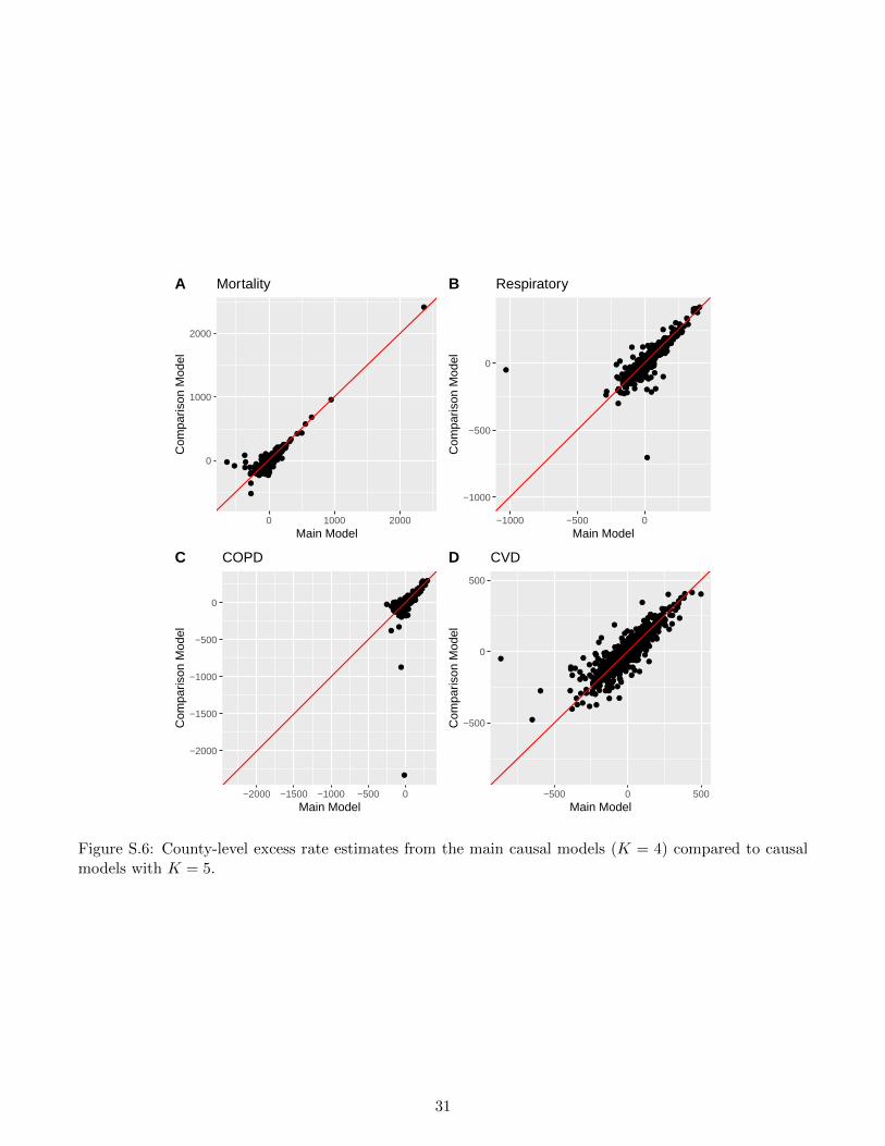
●●●
●●
●
●●
●
●
●●●●●●●
●
●●●●●
●
●●●
●
●●●●●●●●●
●
●●●●●●●
●●
●●●
●●
●●●
●
●●●
●●
●●●
●
●
●
●●●
●●
●
●●●●●●●●●
●●
●●●
●
●●●●●●●●●
●●●
●
●●●●
●●●●●●●●
●●●●●
●●●●
●●●●●●●●●●●●●●●
●
●●●●
●●●●●●●
●●
●
●
●●
●●
●●●
●●●●●●
●●●●●●●
●
●●●●
●●●●●●
●●●●●●
●●●●
●●
●
●●
●●
●
●●
●●●
●●●
●●
●●●●
●●●●
●●●●●●
●●●
●●
●
●●●●●●●●●●●●●●●●
●●●●●
●●
●●●●●
●●●
●●●●●
●
●●
●
●●●●●●
●●●●●
●●●●●
●
●
●●●●●●●
●
●●●●●●●●
●●
●●●
●●
●●●●●●
●
●●●●●●●
●●●●●●●●
●●●
●●●●●●●
●●●●●●●●●●●
●●●●
●
●
●
●●●●
●
●●●●●●
●
●
●●●●
●●
●●●●●
●
●
●●●●
●
●●
●●●●●●●
●●
●●●●●
●●●
●
●●●
●●
●
●
●●●
●●
●
●●
●
●●●●
●●
●●●
●
●●
●●
●
●●●●
●●●●● ●
●
●
●●
●●
●
●
●●●
●●●●●●
●
●●●●●●●
●●●●●●
●
● ●●●●
●
●
●●●●●●
●
●
●●
●●●●
●●●●●●●
●●
●●●●●●●●●●●●●●
●●●
●
●●●●
●
●
●●●●●
●●●
●
●●
●●
●●
●●●●●●
●
●●
●
●●●●●●
●
●●
●●●●
●
●
●●●●●●●●●●●●●●●●●●●●●●●●●●●
●●●●
●
●●
●
●●
●●●
●
●
●●●●●
●
●
●●●●●●●
●
●●●
●
●
●
●●●
●●●●
●●●
●●●●●
●●
●
●●
●●●
●●●
●●
●●●●●●●
●
●●●●
●●
●●●●●●●●●●●●
●
●
●●
●●●●●●●●●●●
●●●●
●●
●●
●●●●●●●●●●●●●●●●●●●●●
●●●●●
●
●●●
●●●●
●
●●
●
●
●●●●●
●●●●●●●●
●●
●
●●●●●●●
●●●●●● ●●●
●
●●
●●
●
●●
●●●●
●●●●●
●●●●
●
●
●
●●
●●●●●●●●●●●●
●●●
●●
●●●●●●●●●●●●
●●●●
●●
●●●
●
●●
●●●
●●●
●
●
●●
●●●●●●
●●
●
●
●●●●●●●
●●●●●
●●
●
●
●●●
●
●●●
●
●
●●●●●●●
●
●●●
●●●
●●●
●●●●
●●●
●
●
●●●● ●●
●
●●
●
●●●●●●●
●●●●●
●●●●●
●●●●●
●●●
●
●
●●
●
●●●●
●●●●●●●●●
●●●●●●●●
● ●●●
●●●●
●●
●●●●●●●●●
●●●●●●●●●
●●●●●●●●●●●●●●●●●●●●●●●
●●
●●●●
●●●●●●●●
●●
●●
●●●
●●●
●●●●●
●
●●●●●●●●
●
●●●●●
●
●
●●●
●●
●●
●
●●●
●
●●●●●●●●
●●●●●●●●●
●
●●
●●●●●●
●
●
●●
●●●
●
●●
● ●
●
●
●
●●●●
●●
●
●●●●
●●
●●
●
●●
●●●
●●
●
●●●●
●●●●
●●
●●
●●
●
●●
●●
●●
●
●●
●
●●●
●
●●
●●●●●
●● ●
●●●●
●
●●●●●●
●●
●
●●
●●●●
●
● ●●●●
●
●●●●●●●
●
●
●
●●
●●
●●●
●●
●●● ●●●
●●
●●
●
●
●●
●
●●
●●●●●●●●
●●●
●●
●
●●
●●●
●
●●●●●●●●
●
●●●●●
●●
●●
●●
●●
●● ●●●●●
●
●
●●
●●●
●● ●●●
●
●
●●●● ●●
●
●●●●●●●
●
●●●●●●●●●
●●●
●●●●●●●●●●
●
●●●●●
●●
●●
●
●●●●
●●●●●●●●
●
●●●
●●
●
●●●●●●●●●●●●
●
●
●●●●●●●●●●●●
●●●●●●●●●●
●●●●●●●●●
●●●●●●●●●●●●●●●●●●●●●●●●●●●
●●●●●
●●●●●●●●●
●●●●●●●
●●●●●●
●
●●●●
●●●
●
●●●●●●
●
●●●
●●●●
●●●
●
●
●●●
●
●●
●●●
●●●
●
●●●●●●●●
●●●
●
●●
●●
●●●●●●●
●●●●●
●●●
●●
●●
●
●●●
●●
●●
●
●●●●
●●●
●●●
●●
●●●●●●●
●●●
●
●
●
●
●●●●
●
●●●●
●●
●
●
●●●●●●
●●●●
●
●
●
●●
●
●●
●
●●
●●●●●
●●
●●●
●
●
●●
●●●●
●
●●
●●●●
●
●
●● ●●
●
●
●
●●●●●
●●●
●●●●●●
●●●
●●●
●
●
●●●●
●●●●●●●●●
●●
●●●
●●●●●●●●●●●
●●
●●●
●
●●
●●●●●
●●
●●
●
●●
●
●
●●●
●●●●●
●●
●●● ●● ●●
●●●
●
●●
●
●●
●●●
●●
●
●●●●●●
●
●● ●
●
●
●
●
●
●●●
●
●
●●●●
●
●
●●
●
●●
●●●●
●
●●●●●●●
●●
●
●
●
●
●●●●●●●
●●
●
●
●
●●●
●●●●
●
●●●
●
●●
●●●
●●●
●
●●
●
●●
●
●●●●●●
●●●●●●●●
●●
●●
●●●
●●
●
●●●●
●●
●
●
●●
●●●
●●●●
●●●
●
●●
●
●●●●●●
●●
●●
●
●
●
●●●●●
●
●●●●●●●
●●
●●
●●●●●●
●●●
●●●●●
●●●●●●
●●●●
●
●●●
●●
●●
●
●●●
●●●
●●●
●●●
●●
●●
●
●
●●
●●●●●●●
●●●●
●●●●●●●
●
●●●●●●●●●●●●●●●●●●●●●●●●●●●●●
●●●
●●●●●●●●●
●●●●
●●
●●●●●
●●●
●●●●●●●●●●
●●●●●
●●●
●●●●●●●●●●●●●●●●●●
●●●●
●●●
●
●●●●●
●
●●●●
●●●
●●●●●0
1000
2000
0 1000 2000Main Model
Com
paris
on M
odel
MortalityA
●●
●●●●●●●
●
●
●●
●
●●
●●●● ●●●●
●●●●●●●
●●
● ●
●●●
●
●●
●●
●●●
●
●●
●
●●●
●
●
●●
●●●
●
●
●●
●
●●
●●
●●
●
●
●●
●
●
●●
●
●
●
●
●
●
●●●
●
●●
●●●
●●
●
●●●
●
●●
●●
●
●
●●
●
●●
●
●●●●
●
●●●●
●●●●●
●●
●
●
●●●
●
●●
●
●●●●●
●
●
●●
●
●●
●
●●●
●●
●●●●●
●●●●●●●●
●●
●
●●●●
●●●
●●●●
●●
●
●●●●●●
●●●
●
●
●
●●
●
●
●
●●
●
●
●
●
●
●●●
●●
●
●
●●
●●●●●
● ●
●●●●
●
●●
●
●●●●●●●●●●
●
● ●● ●
●●
●●
●●●●
●●
●
●●●
●●●●
●
●
●●
●
●
●● ●
●●
●●
●
●
●●●
●
●
●●
●
●●
●
●●●●
●●●
●●
●
●
●●●
● ●●●●
●●
●
●●●●●
●●●
●●●●●●●●●●
●
●
●●●
●
●●●●●
●●
●
●●●●●
●●●
●●●●●●
●●●●●
●
●●
●
●●
●●●●
●
●
●
● ●●●
●●
●●
●
●
●
●●
● ●●
●
●
●
●
●●
●●
●●●●
●
●●●
●●
●
●
●
●
●●●●
●
●
●
●●
●●
●
●
●●●●
●●●●
●
●
●●●
●
●
●
●●
●●
● ●●
●
●
●
●
●
●
●●●●
●●
●
●●
●
●
●
●● ●
●
●
●
●
●
●
●●●
●
●●
●●
●
●
●●
●●●●●●
●●●
●●
●●●
●
●
●
●●
●●
●●●
●
●●●● ●●●●●
●●●●●●
●
●
●
●●●●● ●
●
●●
●
●●
●
●●
●
●
●
●●●
●
●●
●●
●
●●●●●
●●●●
●
●●●●
●
●●
●
●
●●●
●●●
●●●●
●●
●●●
●●●●●●●●●●●
●●●●
●
●●●●●●●
●●●
●
●●
●
●
●●
●
●●
●
●●●
●●
●
●●●
●
●●●●●●
●●●●
●
●
●
●●
●●●
●●
●●
●●
●●●
●
●
●●
●●●●●
●
●●
●
●
●
●●
●●●●
●●
●
●●●●
●●●
●●
●●
●
●●
●
●●●●●●●
●●
●●●●
●
●●
●●●●
●●●●●
●●●●●
●
●●●●●
●●
●
●●●
●
●
●●
●
●
●●
●
●
●
●
●●●●●●
●●●
●● ●
●
●●
●●
●●
●
● ●●
●●●
●
●●●
●
●●
● ●● ●
●●●
●
●
●●● ●●●●●●
●
●●
●●●●●
●
●●
●● ●
●●●●●●
●
●●●
●
●
●
●
●
●
●●●●●
●●●●
●●●
●
●
●
●
●●
●
●
●
●●●
●
●●●●●●
●
●
●
●
●
●
●
●
●
●●
●● ●
●
●
●●
●●
●
●
●
●
●
●
●
●●
● ●●
●
●● ●
●
●
●
●
●●
●
●
●
●
●●●
●
●
●●
●
●
●●●●
●●●
●
●●●
●
●●
●●●●●
●
●
●
●
●●●●●
●●●●●
●●
●●
●
●
●
●●
●●●●
●
●●●●●●●
●
●
●●●●●
●
●
●●●●
●
●
●●
●●●●
●●
●●●●●●●●●●●
●●●
●●●●
●●●●●●●●●●
●●
●
●●
●●●
●●●
●
●
●●●●●●●
●●
●
●
●
●●● ●
●
●
●
●●
●
●●●
●
●●
●
●●●●●
●●
●●
●
●●●
●
● ●
●
●
●
●●●●
●
●
●●●
●●●●
● ●●●
●
●
●
●●
●●
●●●
●
●●
●●
●
●
●
●
●
●
●●●●
●
●●
●●
●●
●●
●●
●●
●
●
●●
●
●
●●●●
●
●●●●●
●●●●
●●●
●
●●
●
●
●
●●●
●●
●
●
●● ●
●
●
●●
●
●
●
●●●
●● ●
●●
●
●●●●
●●●●
●●●
●
●●●
●●
●
●●
●●●●
●
●
●
●
●
●
●
●● ● ●
●●●●
●●●
●
●
●●
●
●●
●
●●
●
●●●
●●
●●●●
●
●
●●
●
●
●●
●●
●●
●
●
●
●● ●●
●
●●●●●
●
●●
●
●
●●●
●●
●●●
●
●●●
●●
●
●
●●
●
●
●
●●
●
●
●
●●●●
●●●
●●●●●●
●●●●●●●
●●
●●●●●
●
●●●●
●●●●●●●
●●
●●●
●
●
●●●
●
●
●●
●●●
●●●●●●●
●●●
●●
●
●●
●●●
●●
●●●●●●●
●
●
●●●
●
●
●●●●●●●●
●●
●●●●
●
●●●●
●●●●●
●
●
●●●
●●●●●●●●●
●●●●●●●●●●
●
●●
●●●●
●
●●●●
●●●
●●●●●
●●●●
●●●●●●●●●●●
●●●
●●●●
●
●
●●●
● ●
●
●
●
●●
●
●●●
●●●
●
●
●
●
●●●
●●
●
●
●●
●
●
●
●
●
●
●
●
●
●●
●
●
●
●●
●●
●
●
●●
●
●●●●
●
●
●●
●
●
●
●●
●●●
●
●● ●●
●●
●●●●●
●●●●
●
●
●●●●●
●●●
●
●
●
●
●●
●
●
●
● ●●●
●
●
●●●
●
●
●
●
●
●●●
●●●●
●
●
●●
●
●●
●
●●●
●
●
●
●
●
●
●●
●●●●
●
●
●●
●
●
●
●●
●
●●
●
●
●
●
●
●●
●
●●
●
●●●
●
●●
●●●●
●●
●
●●
●
●
●
●●
●●
●●
● ●
● ●●●
●●
●
●●●
●
●●
●
●
●
●
●
●
●●●●
●
●
●
●
●●
●
●●
●●
●●
●
●
●
●●
●
●
●
●●
●
●●
●
●
●
●
●
●
●
●●
●●●●
●●● ●
●●
●●●●●●
●
●●
●●●●●●●●
●
●
●
●
●
●
●
●
●●●
●●
●●
●
●●
●●
●●
●
●●●
●● ●●●●●●
●
●●●
●
●
●
●●
●●
●
●
●●
●
●●
●
●
●
●
●
●●
●
●
●
●
●●
●
●
●●
●●
●
●●
●
●●
●
●●
●
●●●●
●●●
●
●
●●
●
●●
●
●
●
●
●
●
●
●
●
●
●●
●●●
●●
●
●
●●
●
●●
●
●●●
●●
●
●
●
●
●●●
●
●
●
●
●
●
●
●
●
●●●
●
●
●●
●
●
●
●
●●
●●
●●
●●●
●●
●
●●●●
●
●●●●
●
●
●
●●
●●●●
●
●
●
●
●
●
●
●●
● ●
●
●
●
●●
●●
●●
●
●
●●
●
●
●
●
●
●
●●●
●●
●
●
●
●
●
●●
●●
●●●●●●●
●●●
●●
●●●●●
●●●●●●●●
●●●
●●●●●
●●●
●●●●●
●●●
●●● ●●●
●●●●●
●●●●●
●
●
●●●
●
●
●●●
●
●●●
●●
●
●●●●●●●
●●
●●●
●●●●●
●●
●●●
●
●●
●
●●
●●
●●
●●
●
●●
●●●●●
●●
−1000
−500
0
−1000 −500 0Main Model
Com
paris
on M
odel
RespiratoryB
●●●●●●●●●●●●●●●●●
●●●●●●●●
●●●●●●
●●●●●●●●●●●●
●●●●●●●●●●●●
●●●●
●●
●●●
●
●●
●●
●●●●●●●●●●●●●●●
●●
●●●●●●●●●●●●●●
●●
●
●●●●●●●●●
●●●●●●●●●●●●●●●
●●●●●●●
●●●●●●●●●●●●●●●●●●●
●●●●●●●●●●●●●●●●●●
●●●●●●●●●●●●
●●●●●●●●●●●●●●●●●●
●●●●
●
●
●●●●●●●●●●●●●●●●●●●●●●●●
●●
●
●●●●●●●●●●●●●●●●●●●●●●
●●●●●
●●
●●●●●●●
●●●
●●●●●
●●
●
●●
●●●●●●●●●●●
●●●●●●●
●●●●
●●●●●●●●●●
●●●●●●●●●●●●●●●●●●
●●
●●●
●●
●●●●●●
●●●●●●●●●●
●●●●●
●●
●●●●●●●●●●●●
●
●
●●
●●
●●
●
●
●
●●●●●●●
●●
●●●●
●●
●● ●● ●
●●●●●●●●
●●●●●●●●
●●●
●●●●
●●●
●●●
●
●●●
●
●●●●●●●●●●●●●●
●
●●●●●
●●●●●
●
●●●●●
●●
●
●●●●●
●
●●●●
●●●● ●●●●●●●●●●●●●●●●
●●●●●
●●●●●●●●●●●●●●●●●●●●●●●
●●●●●
●●●●●
●●●●●
●●●●●
●●
●●●
●●
●●●●●●
●●●●●
●●●
●●●●
●●●
●
●●●●●●●●●●●●
●●●●●●●
●●●●●●●●●●●●●●●●●●●●●●●●●●●●●●●●●●●●●●
●
●●●
●●●●●●●●●●●●
●●●●●●●●●●●●●●●●●
●
●●●
●●●●
●●
●●
●●●●●●●●●●●●●●●●●●●●●●●●●●●●●●●●●●●●●●●●●●●●●●●●●●●●●●●●●●●●●●●
●●●●●●●●●●
●●●●●●
●● ●●●●●●●●
●
●
●●●●●●●●
●
●●●●●●●●●●●
●
●●●●
●●●●
●●●
●
●●●●●●●
●● ●
●
●●●●●
●●
●●●●●●●●●●
●●●
●●
●●
●●●●●●●●●●●●●●●●
●●●●●●●●●●●●●●●●●●●
●●●●●●●●●
●●●
●
●●
●●
●●
●●●●●
●●●●●
●●●●●●
●●
●
●●●● ●●●●●
●●●●●
●●●●●●●●●●●●●●●●●●●●●●
●
●●●●●
●●●●●●●●●●●●●●
●
●●●●●●●●●●●●●●●●
●●●●
●
●●●●●●●
●●●●●●●●●●●●●●●●●●●●●●●●●●●●●●●●●●●●●●●●●●●●●●●●
●●●●●●●●
●
●●
● ●●●
●●●
●
●●●●●●●●●●●●●
●●●●●●
●●●●●●●
●●
●●●●●●●●●●●
●●●●●●●
●
●●●
●
●●
●●●
●
●●●●
●●●
●
●●
●●●●●●●●
●
●●●●
●●●●●
●●●●●●●●
●
●
●●●●●●●
●●
●●●
●●●
●●●●●●
●●●
●●●●
●●●●●●●
●●●●●●
●●●●●●●●●●●●●●
●●●●
●●●
●●●●●●●●
●●●
●●
●
●●●●●●●●●●
●
●●●
●
●●●●●●●●●
●
●●●●●●
●●●●●●●●●
●●●
●
●●●●●●
●●●●●●●●●●
●●●●●●●
●
●●●●
●●●●●●●●
●●
●●●
●●●●●●●●
●●●●●●
●●●●●●●●●●●●●●
●
●●●●●●●●
●●●●●●●●
●●●
●●●
●●●●●
●●●●●●●●●●●●●
●
●●●●●●●●●●●●●●
●●●●●●●●●●●●●●●●●●●●●●●●●●●●●●●●●
●●●●●●●●●●●●●●●●●●●●●●●
●●●●●●●●●●●●
●●●●●●●●●●●●●●●●●●●●●●●●●●●●●
●●
●●●●●●●
●●
●●
●●
●
●
●●●
●
●●●●
●
●●●●●●●
●
●
●●●●●●●●●●●●●●●●●●●
●●●●●
●●●●
●
●
●●●●●●●●
●●●
●●●●●●●●●●●●●●
●●●●
●●●●●
●●●●
●●●●●●
●●●●●●●●●●●●●●●●●
●●
●
●●
●
●●
●
●●●●●●●●●
●●●●●
●
●
●●●●●
●●●●
●●●●
●●●●
●●
●●●●●●
●●●●
●●●●●●
●●●●●
●●●
●●●●●
●●●●●●
●●●
●●●●
●
●
●
●
●●●
●●●●●
●●●●
●●●
●●
●●●
●●
●●●
●
●●●●
●●●●
●●●●
●●●●●●●●●●
●
●●●●●●●●●●●●●●●●●●●●
●●
●●●●
●●●●●●●●●●●
●●●
●●●●●●●●●●
●●●●●●●●●
●
●●
●●●●●●●
●●
●
●●
● ●
●●
●
●
●
●●
●
●●
●●
●●
●●
●●●
●
●
●●●
●●
●●●●●
●
●
●●●●●
●
●
●●●●
● ●
●
●
●●●●
●●●●●● ●
●●●
●
●●●●●●
●●●
●●●
●●
●●
●
●●●●●●●●
●●●
●
●●●●●●●●
●●●
●●●●●●●
●●●●●●●●●
●●
●●●●
●●●●
●
●
●●●●
●●●●●●
●●
●●●●● ●
●●
●●
●●●●●●●
●●
●●●●●●●
●●●●●●●●●●●●●●●●●●●●●●●●●●●●●●●●●●●●
●●●●●●●●
●●●●●●●●●●●●●●●●●
●●●●●
●●●●●
●●●●●●
●●●●●●●●●●●●●●●●●
●●●●●●●
●●
●●
●●●●●●●●●●● ●●●●●
−2000
−1500
−1000
−500
0
−2000 −1500 −1000 −500 0Main Model
Com
paris
on M
odel
COPDC
●●●
●
●
●●
●
●
● ●
● ●
●
●
●
●
●
●
●
●
●●
●
●
●
●
●
●
●●
●●
●
●
●
●●
●
●
●
●
●●
● ●●
●
●
●
●●
●● ●
●
●
●
●
●●
● ●
●
●
●
●
●
●
●●
●
●
●●
●●●●
●
●
●
●●
●
●●
●
●
●
●
●●●●
●
●●
●
●●●
●
●●
●
●●●
●
●●●
●●●
●●
●
●●
●
●●
●●●
●
●●
●●●●
●
●●●
●●●
●
●
●
●
●●
●● ●
●●●
●
●
●
●●
●●
●
●●
●
●
●
●
●
●
●
●
●
●●
●
●
●
●●
●●●●●
●●
●●●
●
●
●●●
●●
●
●●
●
●
●
●
●●
●
●
●●
●●
●●●
●
●
●
● ●
● ●
●
●
●●●●
●●
●●●
●●●●●●
●●
●●●●
●
●●
●●●
●
●
●
●
●
●
●
●
●
●
●●
●
●
●
●●
●
●
●● ●
●
●
●
●
●●
●
●
●
●
●
●●
●
●
●●
●●●
●
● ●
●●
●
●
●
●
●
●
●
●
●
●
●
●●
●●●●
●
●
●
●●
●
●
●
●●
●●●●
●
●●
●●
●
●
●
●
●
●
●
●●●●●
●
●
●
●●
●
●●●●●
●
●
●
●
●
●
●●●●
●
●●●
●
● ●●
● ●
●
●
●
●
●
●●
●
●
●
●
●
●
● ●
●●
●
●
●
●
●
●
●
●
●
●
●
●
●
●
●
●●●●
●
●
●
●
●
●●
●●
●
●
●
●
●
●
● ●●●
●
●
●●
●
●●●
●
●
●
●
●
●
●●
●
●
●
●
●
●
●●
●
●●
●
●
●
●●
●●
●
●
●
●
●
●●
●
●
●
●●
●
●●
●●●●
●
●
●
●
●
●
●
●
●●●
●●
●
●
●●
●
●
●
●●
●
●
●●
●
●●
●●
●
●●
●
●●
●
●●●●
●●
●●
●●●
●●
●
●
●
●●
●
●
●●
●
●
●
●
●●
●
●
●
●
●
●
●●●●●
●
●
●
●
●
●●
●
●
●
●
●
●
●●●●
●●
●
●
●
●●●
●●
●●●
●
●●
●●●
●
●●
●
●
●
●●●
●●
●●
●●●
●
●
●
●
●
●
●
●
●
●
●
● ●
●
●
●
●
●
●
●●
●
●
●
●
●
●●
●
●
●
●●
●●
●●
●●●
●●●●●●
●●
●●
●
●
●
●
●
●
●
●
●
●●
●
●
●
●●
●
●●
●
● ●
●
●
●
●●
●
●
●●
●●
●
●●
●
●
●
●
●
●●
●●
●
●
●
●●
●●
●
●●●
●
●●
●●
●
●
●●
●●●●
●●
●●●●●
●
●●●
●●
●●
●●
●●●
●
●●
●
●
●
●
●
●●
●
●●●●
●●
●
●●
●
●
●
●●
●
●●●
●
●
● ●●● ●●●●●●●
●●●●
●
●●
● ●●●
●
●●
●
●
●●
●●
●
●
●
● ●
●●
●
●
●
●
● ●●●●●
● ●●
●
●
●
●
●●
●
●
●
●
●
●
●
●
●●
●
●●
●
●
●
●
●●
●
●●
●
●●
●
●
●
●
●
●●
●
●●
●●
●
●
●●
● ●
●
●
●
●●
●
●
●
●
●
●
●●
●●
●
●
●●
●
●
●●
●
●●● ●
●
●
●
●
●
●●
●
●
●
●
●●●
● ●
●●
●
●●
●
●●
●●
●
●
●●
●●
●
●
●
●
●
●●●
●
●●
●
●
●●
●
●●
●
●●
●
●
●
●
●
●
●●
●
●●
● ●
●
●●●●
●●●
●
●
●●
●●
●
●
●
●
●
●
●
●
●
●●●●
●●●●
●
●
●●●●●●●●●●●●●
●●
●●●
●●●
●●●●
●
●
●
●
●
●
●
●
●●
●
●
●
●
●●
●
●
●
●
●
●
●
●●
●
●
●●
●
●
●
●
●●
●
●●
●
● ●
●
●
●
●●
●
●
●
●
●
●●●●
●
●●
●
●
●●
●●
●
●●
●
●
● ●
●●
●●●
●
●
●
●
●
●
● ●●
●
●
●
●●●●
●
●●
●
●
●
●
●
●
●●
●
●
●
●● ●●
●
●
●
●
●
●
●
●
●
●
●
●
●
●●
●
●
●
●●
●●
●
●
●
●
●
●
●●
●
●●●
●
●
●
●●
●●
●
●
●
●
●
●●
●
●
●
●
●
●
●
●
●
●
●●
●●
●
●●
●●●●
●
●●●●
●
●●
●
● ●
●
●●
●
●
●
●
●
●
●● ●
●
●
●
●
●●●●●
●
●●●
●
●
●
●
●
●
●●
●
●●●
●
●
●
●●
●
●
●
●
●
●
●●
●
●
●
●●
●
●
●●
●
●
●
●
●● ●●●
●●●●●
●
●●
●
●
●●
●
●
●●
●
●
●
●
●
●●
●●
●
●
●
●●
●●
●●●
●
●●
●●
●
●
●
●
●
●●
●●●●
●
●●●●●
●
●●●
●
●
●●●
●●●
●
●
●●●
●
●
●
●●
●
●
●●
●
●●
●●
●
●
●●●
●
●
●
●
●
●
●
●
●●●●●
●
●●
●●●
●
●
●
●
●●
●
●
●
●●●●●●●●
●
●●●●
●●
●
●●
●●
●●●●
●
●●●
●●●●●●● ●●●●●●●
●
●●●●
●
●
●●
●●●●
●●●●●
●
●●
●●
●
●
●●●●
●
●●●
●
●
●● ●●●
●●●●
●
●●
●
●
●●
●●
●
●●
●●
●●●
●
●
●
●
●
●
●
●
● ●●
●
●
● ●
●
●
●
●
●●
●●
●●●
●
●
●●
●
●
●
●
●
●
●
●●●
●
●
●
●
●
●●●
●●
● ●
●
●
●
●
●●
●
●
●
●●
●
●●
●
●●
●●●
●
●
●
●
●
●
●●
●
●
●
●
●●
●
●
●
●
●
●
●●●
●
●
●●
●
●
●
●
●● ●
●
●
●
●
●
●
●
●
●
●●
●●
●●
●
●
●●
●●
●●
●●
●
●●
●
●●
●
●
●
●●
●
●
●●
●
●●
●●
●
●
●
●
●
● ●●
●●
●
●
●
●
●●
●
●●
●●
●●
●
●
●
● ●●
●
●
●
●
●
●●
●●
●●●
●
●
●●
●
●
●
●
●●
●●
●
●
●
●
●
●
●
●● ●
●
●
●
●
●
●
●
●●●
●●
●
●
●
●●
●●
●
●
● ●
●
●●●
●●● ●●●●●
●
●
●
●
●●●
●
●
●●
●
●● ●●
●●
● ●●●●
●
●
●
●
●●●
●
●
●
●
●
●
●
●
●
●
●
●
●
●
●●●
●●●●●●
●
●●
●
●
●●●
●
●●●
●●
●
●
●
●
●
●
●
●●●●
●
●●●
●
●
●
●
●
●
●
●
●●
●●
●●
●●
●
●
●
●
●
●
●
●
●
●●●
●
●
●
●●●
●
●
●
●
●
●
●
●●
●
●●●●●
●
●
●●
●●
●
●
●●
●●●●
●
●
●
●
●
●●
●
●
●
●●
●
●●
●
●
●
●
●●
●
●
●
●
●
●
●
●
●
●
●
●
●●●●
●
●
●
●
●●
●
●
●●
●
●
●●
●
●●
● ●
●
●
●
●
●●
●
●
●●
●
●●●
●
●●●●●
●
●
●●●
●
●
●●●
●
●
●
●●
●
●●
●●
●●
●
●●●
●●●●
●●●
●
●●●
●●●
●
●●
●●
●●●
●
●●
●
● ●●
●●●●
●●
●●
●●
●●
●●●
●
●
●
●
●●
●●●●
●●●●
●●●●
●
●●
●●
●●
●
●
●
●●
●
●
●
●
●●●
●●
●
●●
●
●●
● ●
●●
●●
●
●●●●
●
●
●
●
●●●●
●●
●
●
●
● ●
●
●
●
●●●●
−500
0
500
−500 0 500Main Model
Com
paris
on M
odel
CVDD
Figure S.6: County-level excess rate estimates from the main causal models (K = 4) compared to causalmodels with K = 5.
31

S.8.2 Predictive model
TCs can bring extreme rainfall amounts and flooding, and we hypothesize that these exposures may causeincreases in some adverse health events. Currently, the hurricaneexposuredata package contains TCrainfall data only through the year 2011. Due to the missing precipitation data for later years, we do notinclude this variable in our main predictive models, but here, as an additional sensitivity analysis, we fitthe predictive models only using TCs in years 2011 and prior with precipitation as a predictor. As in theprimary models, we fit regression models excluding state indicators but including all other predictors, withrestricted cubic splines on windspeed and year. We also include a restricted cubic spline on county-levelcumulative TC precipitation, measured over a four-day window starting two days prior to the storm’sclosest approach to the county. The precipitation splines from the fully modularized models are shown inFigure S.7. After adjusting for all the other predictors, there appears to be weak or no effect of precipitationon any of the health outcomes evaluated here. Thus, the inference and predictions from our model areunlikely to be sensitive to the inclusion of precipitation information.
|| ||| || || || || | || || || ||| || | ||| || || | |||| || || || || | | || ||| || ||| |||| | || |||| || || | || | |||| ||| | ||| || | | || || | || || || || || ||| ||| |||| ||||| || ||| | || || ||||| | |||| ||| | || || ||| | || |||||| |||| |||| | || ||||| | | || ||||| || || | ||| || | || |||| | || | ||| ||| ||| || ||||| | || ||| ||||| ||||| | |||| | || || ||| || | | ||| || ||| ||| || ||| || || ||| || ||| ||| || || ||||| ||| ||| || || |||| || || ||||| || ||| ||| | || ||| || | | || ||| || | || || || || ||| | ||| || ||| || ||| ||| | || || ||| || || || |||| | || | ||| ||| || || ||| || || || || || ||| ||| ||| || ||| | || || || || || ||| | ||| || | |||||| || | | ||| ||||| ||| || | || || ||| || | ||| | || | ||| | |||| ||| | | ||| | ||| || | || || |||||| | || ||| | | ||| || || || | ||| ||| || | ||| | | |||| |||||| ||||| ||| | | |||||| ||| || | | | | || || || | |||| | ||||| | | ||| || ||| || |||| | || |||| || || ||| || | ||| || || || || | || || ||| | ||| ||| || || ||| | || | || || | || || ||| | | || || ||| || || ||| | |||| || || ||| || || | ||| | || || || || || ||| || |||| | | || || || || || || | || || | |||| ||| ||| | || |||| | || || |||| | | | |||| || || || | ||| | ||| ||||| || ||| ||| || |||||| || || || || | || ||| || |||| || || ||| ||| |||| ||| || | ||||| || | || || || || |||| || | | ||||| ||| || ||||| || | ||| | | || || | || | || ||| | ||| | || ||| | || ||| || || || || ||| || | || || || || || || | || | | || | | || || | || ||| || | ||| | | || || || | | |||| | | || || || ||| ||||| | | |||| | || | || || | | ||| ||| ||| ||| || || ||||| || | || | || || || ||| || ||| || ||| || || | || ||| | ||| | ||| | || || || | | ||| | | || ||| ||| | || || || | ||| | | || | | || || | | || || || || || ||| || | || || || | || ||||| |||| ||| || | || | ||| || || | ||| | | ||| || || || | || |||| || || | ||| || ||| || | |||||| || ||| || || || || || |||| ||| || || ||| | || ||| | || | || || || ||| | || | || | ||| ||| || | || || || ||||| |||| ||| || | | || || ||| || | |||| || ||| || || || || || || |||| || |||| | | || | || || || | ||| ||| || | || | || || ||| || | || ||| || || |||| || || || || || || || ||| || ||| || ||| | || || | || ||| || || ||| ||| || | ||| | || || || || | || || || || | || || |||| | || | |||| |||| ||||| | || ||| | |||| ||| ||| | ||| |||| ||||||| | | ||||| | | | || | || || | |||| ||| || || | | ||| || ||| | || || || ||| | || | | |||| | ||| | || ||| || || ||| | | ||| | || | || ||||| || | ||| | || | ||| || ||| || ||| | |||| || |||| || || | || | || | ||| ||||| || | | || | || | ||| | ||| || | || || || ||| || || ||| | ||| | || | || | || ||| ||| ||| || ||| ||| | | || ||| ||| || || || | ||| || | || ||| | ||| || || || || | || | ||| || ||| || || || | | ||| || || ||| | || | ||| || |||||| | ||| || | | || || || |||| | | || || | ||| | || || || || | || || || ||| | || | || || ||| || ||| ||| | | || || || | | | | || || || || || |||| || || || ||| || || |||| || || || | || || | || || || || || | || || ||| || ||| || || || || | | | ||| || || | || || || || | || || || | || || || || || | ||| || || |||| || || | || || || | ||| || || || | || || || |||| || || || || ||| || || || || |−40
0
40
80
0 100 200 300Cumulative Precipitation
Cha
nge
in M
orta
lity
A
|| ||| || || || || | || || || ||| || | ||| || || | |||| || || || || | | || ||| || ||| |||| | || |||| || || | || | |||| ||| | ||| || | | || || | || || || || || ||| ||| |||| ||||| || ||| | || || ||||| | |||| ||| | || || ||| | || |||||| |||| |||| | || ||||| | | || ||||| || || | ||| || | || |||| | || | ||| ||| ||| || ||||| | || ||| ||||| ||||| | |||| | || || ||| || | | ||| || ||| ||| || ||| || || ||| || ||| ||| || || ||||| ||| ||| || || |||| || || ||||| || ||| ||| | || ||| || | | || ||| || | || || || || ||| | ||| || ||| || ||| ||| | || || ||| || || || |||| | || | ||| ||| || || ||| || || || || || ||| ||| ||| || ||| | || || || || || ||| | ||| || | |||||| || | | ||| ||||| ||| || | || || ||| || | ||| | || | ||| | |||| ||| | | ||| | ||| || | || || |||||| | || ||| | | ||| || || || | ||| ||| || | ||| | | |||| |||||| ||||| ||| | | |||||| ||| || | | | | || || || | |||| | ||||| | | ||| || ||| || |||| | || |||| || || ||| || | ||| || || || || | || || ||| | ||| ||| || || ||| | || | || || | || || ||| | | || || ||| || || ||| | |||| || || ||| || || | ||| | || || || || || ||| || |||| | | || || || || || || | || || | |||| ||| ||| | || |||| | || || |||| | | | |||| || || || | ||| | ||| ||||| || ||| ||| || |||||| || || || || | || ||| || |||| || || ||| ||| |||| ||| || | ||||| || | || || || || |||| || | | ||||| ||| || ||||| || | ||| | | || || | || | || ||| | ||| | || ||| | || ||| || || || || ||| || | || || || || || || | || | | || | | || || | || ||| || | ||| | | || || || | | |||| | | || || || ||| ||||| | | |||| | || | || || | | ||| ||| ||| ||| || || ||||| || | || | || || || ||| || ||| || ||| || || | || ||| | ||| | ||| | || || || | | ||| | | || ||| ||| | || || || | ||| | | || | | || || | | || || || || || ||| || | || || || | || ||||| |||| ||| || | || | ||| || || | ||| | | ||| || || || | || |||| || || | ||| || ||| || | |||||| || ||| || || || || || |||| ||| || || ||| | || ||| | || | || || || ||| | || | || | ||| ||| || | || || || ||||| |||| ||| || | | || || ||| || | |||| || ||| || || || || || || |||| || |||| | | || | || || || | ||| ||| || | || | || || ||| || | || ||| || || |||| || || || || || || || ||| || ||| || ||| | || || | || ||| || || ||| ||| || | ||| | || || || || | || || || || | || || |||| | || | |||| |||| ||||| | || ||| | |||| ||| ||| | ||| |||| ||||||| | | ||||| | | | || | || || | |||| ||| || || | | ||| || ||| | || || || ||| | || | | |||| | ||| | || ||| || || ||| | | ||| | || | || ||||| || | ||| | || | ||| || ||| || ||| | |||| || |||| || || | || | || | ||| ||||| || | | || | || | ||| | ||| || | || || || ||| || || ||| | ||| | || | || | || ||| ||| ||| || ||| ||| | | || ||| ||| || || || | ||| || | || ||| | ||| || || || || | || | ||| || ||| || || || | | ||| || || ||| | || | ||| || |||||| | ||| || | | || || || |||| | | || || | ||| | || || || || | || || || ||| | || | || || ||| || ||| ||| | | || || || | | | | || || || || || |||| || || || ||| || || |||| || || || | || || | || || || || || | || || ||| || ||| || || || || | | | ||| || || | || || || || | || || || | || || || || || | ||| || || |||| || || | || || || | ||| || || || | || || || |||| || || || || ||| || || || || |−40
−20
0
20
40
60
0 100 200 300Cumulative Precipitation
Cha
nge
in R
espi
rato
ry
B
|| ||| || || || || | || || || ||| || | ||| || || | |||| || || || || | | || ||| || ||| |||| | || |||| || || | || | |||| ||| | ||| || | | || || | || || || || || ||| ||| |||| ||||| || ||| | || || ||||| | |||| ||| | || || ||| | || |||||| |||| |||| | || ||||| | | || ||||| || || | ||| || | || |||| | || | ||| ||| ||| || ||||| | || ||| ||||| ||||| | |||| | || || ||| || | | ||| || ||| ||| || ||| || || ||| || ||| ||| || || ||||| ||| ||| || || |||| || || ||||| || ||| ||| | || ||| || | | || ||| || | || || || || ||| | ||| || ||| || ||| ||| | || || ||| || || || |||| | || | ||| ||| || || ||| || || || || || ||| ||| ||| || ||| | || || || || || ||| | ||| || | |||||| || | | ||| ||||| ||| || | || || ||| || | ||| | || | ||| | |||| ||| | | ||| | ||| || | || || |||||| | || ||| | | ||| || || || | ||| ||| || | ||| | | |||| |||||| ||||| ||| | | |||||| ||| || | | | | || || || | |||| | ||||| | | ||| || ||| || |||| | || |||| || || ||| || | ||| || || || || | || || ||| | ||| ||| || || ||| | || | || || | || || ||| | | || || ||| || || ||| | |||| || || ||| || || | ||| | || || || || || ||| || |||| | | || || || || || || | || || | |||| ||| ||| | || |||| | || || |||| | | | |||| || || || | ||| | ||| ||||| || ||| ||| || |||||| || || || || | || ||| || |||| || || ||| ||| |||| ||| || | ||||| || | || || || || |||| || | | ||||| ||| || ||||| || | ||| | | || || | || | || ||| | ||| | || ||| | || ||| || || || || ||| || | || || || || || || | || | | || | | || || | || ||| || | ||| | | || || || | | |||| | | || || || ||| ||||| | | |||| | || | || || | | ||| ||| ||| ||| || || ||||| || | || | || || || ||| || ||| || ||| || || | || ||| | ||| | ||| | || || || | | ||| | | || ||| ||| | || || || | ||| | | || | | || || | | || || || || || ||| || | || || || | || ||||| |||| ||| || | || | ||| || || | ||| | | ||| || || || | || |||| || || | ||| || ||| || | |||||| || ||| || || || || || |||| ||| || || ||| | || ||| | || | || || || ||| | || | || | ||| ||| || | || || || ||||| |||| ||| || | | || || ||| || | |||| || ||| || || || || || || |||| || |||| | | || | || || || | ||| ||| || | || | || || ||| || | || ||| || || |||| || || || || || || || ||| || ||| || ||| | || || | || ||| || || ||| ||| || | ||| | || || || || | || || || || | || || |||| | || | |||| |||| ||||| | || ||| | |||| ||| ||| | ||| |||| ||||||| | | ||||| | | | || | || || | |||| ||| || || | | ||| || ||| | || || || ||| | || | | |||| | ||| | || ||| || || ||| | | ||| | || | || ||||| || | ||| | || | ||| || ||| || ||| | |||| || |||| || || | || | || | ||| ||||| || | | || | || | ||| | ||| || | || || || ||| || || ||| | ||| | || | || | || ||| ||| ||| || ||| ||| | | || ||| ||| || || || | ||| || | || ||| | ||| || || || || | || | ||| || ||| || || || | | ||| || || ||| | || | ||| || |||||| | ||| || | | || || || |||| | | || || | ||| | || || || || | || || || ||| | || | || || ||| || ||| ||| | | || || || | | | | || || || || || |||| || || || ||| || || |||| || || || | || || | || || || || || | || || ||| || ||| || || || || | | | ||| || || | || || || || | || || || | || || || || || | ||| || || |||| || || | || || || | ||| || || || | || || || |||| || || || || ||| || || || || |
−20
0
20
0 100 200 300Cumulative Precipitation
Cha
nge
in C
OP
D
C
|| ||| || || || || | || || || ||| || | ||| || || | |||| || || || || | | || ||| || ||| |||| | || |||| || || | || | |||| ||| | ||| || | | || || | || || || || || ||| ||| |||| ||||| || ||| | || || ||||| | |||| ||| | || || ||| | || |||||| |||| |||| | || ||||| | | || ||||| || || | ||| || | || |||| | || | ||| ||| ||| || ||||| | || ||| ||||| ||||| | |||| | || || ||| || | | ||| || ||| ||| || ||| || || ||| || ||| ||| || || ||||| ||| ||| || || |||| || || ||||| || ||| ||| | || ||| || | | || ||| || | || || || || ||| | ||| || ||| || ||| ||| | || || ||| || || || |||| | || | ||| ||| || || ||| || || || || || ||| ||| ||| || ||| | || || || || || ||| | ||| || | |||||| || | | ||| ||||| ||| || | || || ||| || | ||| | || | ||| | |||| ||| | | ||| | ||| || | || || |||||| | || ||| | | ||| || || || | ||| ||| || | ||| | | |||| |||||| ||||| ||| | | |||||| ||| || | | | | || || || | |||| | ||||| | | ||| || ||| || |||| | || |||| || || ||| || | ||| || || || || | || || ||| | ||| ||| || || ||| | || | || || | || || ||| | | || || ||| || || ||| | |||| || || ||| || || | ||| | || || || || || ||| || |||| | | || || || || || || | || || | |||| ||| ||| | || |||| | || || |||| | | | |||| || || || | ||| | ||| ||||| || ||| ||| || |||||| || || || || | || ||| || |||| || || ||| ||| |||| ||| || | ||||| || | || || || || |||| || | | ||||| ||| || ||||| || | ||| | | || || | || | || ||| | ||| | || ||| | || ||| || || || || ||| || | || || || || || || | || | | || | | || || | || ||| || | ||| | | || || || | | |||| | | || || || ||| ||||| | | |||| | || | || || | | ||| ||| ||| ||| || || ||||| || | || | || || || ||| || ||| || ||| || || | || ||| | ||| | ||| | || || || | | ||| | | || ||| ||| | || || || | ||| | | || | | || || | | |||| || || || ||| || | || || || | || ||||| |||| ||| || | || | ||| || || | ||| | | ||| || || || | || |||| || || | ||| || ||| || | |||||| || ||| || || || || || |||| ||| || || |||| || ||| | || | || || || ||| | || | || | ||| ||| || | || || || ||||| |||| ||| || | | || || ||| || | |||| || ||| || || || || || || |||| || |||| | | || | || || || | ||| ||| || | || | || || ||| || | || ||| || || |||| || || || || || || || ||| || ||| || ||| | || || | || ||| || || ||| ||| || | ||| | || || || || | || || || || | || || |||| ||| | |||| |||| ||||| | || ||| | |||| ||| ||| | ||| |||| ||||||| | | ||||| | | | || | || || | |||| ||| || || | | ||| || ||| | || || || ||| | || | | |||| | ||| | || ||| || || ||| | | ||| | || | || ||||| || | ||| | || | ||| || ||| || ||| | |||| || |||| || || | || | || | ||| ||||| || | | || | || | ||| | ||| || | || || || ||| || || ||| | ||| | || | || | || ||| ||| ||| || ||| ||| | | || ||| ||| || || || | ||| || | || ||| | ||| || || || || | || | ||| || ||| || || || | | ||| || || ||| | || | ||| || |||||| | ||| || | | || || || |||| | | || || | ||| | || || || || | || || || ||| | || | || || ||| || ||| ||| | | || || || | | | | || || || || || |||| || || || ||| || || |||| || || || | || || | || || || || || | || || ||| || ||| || || || || | | | ||| || || | || || || || | || || || | || || || || || | ||| || || |||| || || | || || || | ||| || || || | || || || |||| || || || || ||| || || || || |−100
−50
0
50
0 100 200 300Cumulative Precipitation
Cha
nge
in C
VD
D
Figure S.7: Relationship between cumulative precipitation and excess rate per 100,000 of mortality (A),respiratory hospitalizations (B), COPD hospitalizations (C), and CVD hospitalizations (D).
32

S.9 Additional tables and figures
Table S.3: Definition of estimands. s = {1, ..., S} indexes TCs and i ∈Ws indexes treated counties for TCs.Name Definition Formula
Individual excess events (IEE) County-level excess events at-tributable to a single TC s over thetreatment period
θsi =∑
t≥T0[Ysit(1)− Ysit(0)]
Individual excess rate County-level excess event rate (per100,000 population) attributable toa single TC s over the treatment pe-riod
θ∗si = 100000× (θsi/piT )
TC-specific excess events Cumulative excess events summedacross all counties impacted by asingle TC s
∑i∈Ws
θsi
TC-specific excess rate Excess event rate (per 100,000 pop-ulation) across all counties impactedby a single TC s
100000× (∑
i∈WspiT )−1
∑i∈Ws
θsi
Total excess events (TEE) Cumulative TC-attributable excessevents summed over all TCs andcounties in the study
TEE =∑S
s=1
∑i∈Ws
θsi
Average excess rate (AER) Average of the TC-attributable ex-cess rates across all county-level TCexposures in the study
AER = 1Ntotal
∑Ss=1
∑i∈Ws
θ∗si,
Ntotal =∑S
s=1 |Ws| is the total num-ber of county-level TC exposures inour analyses
33
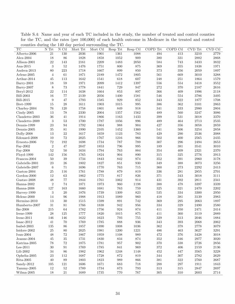
Table S.4: Name and year of each TC included in the study, the number of treated and control countiesfor the TC, and the rates (per 100,000) of each health outcome in Medicare in the treated and controlcounties during the 140 day period surrounding the TC.
TC N Trt N Ctl Mort Trt Mort Ctl Resp Trt Resp Ctl COPD Trt COPD Ctl CVD Trt CVD Ctl
Alberto-2006 21 130 2036 1901 1361 1088 494 413 3210 2779Alex-2004 18 86 1828 1858 1052 909 380 331 2882 2868Allison-2001 22 143 2161 2209 1483 2050 584 743 3433 3832Ana-2015 3 52 1476 1751 800 875 369 355 1838 1971Andrea-2013 80 223 1718 1667 899 850 373 356 2059 1897Arlene-2005 4 61 1871 2189 1472 1805 561 669 3010 3288Arthur-2014 45 113 1642 1541 618 607 248 251 1864 1579Barry-2001 18 59 1971 2099 1412 1397 556 554 3418 3552Barry-2007 8 73 1778 1841 729 947 272 370 2187 2616Beryl-2012 22 114 1638 1664 853 897 366 409 1996 2118Bill-2003 16 77 2139 2056 1400 1581 546 554 3786 3495Bill-2015 9 47 1793 1585 929 852 343 322 1877 1708Bret-1999 15 28 1611 1903 1015 995 386 362 3101 2863Charley-2004 76 120 1758 1801 849 918 341 333 2980 2804Cindy-2005 13 78 2330 2004 1357 1562 489 560 3247 3086Claudette-2003 36 41 1914 1866 1163 1433 399 531 3018 3370Claudette-2009 3 53 1700 1787 1056 996 489 464 2713 2535Dennis-1999 23 94 1792 1864 988 904 427 356 3058 2859Dennis-2005 35 81 1990 2105 1452 1360 541 506 3254 2858Dolly-2008 13 22 1617 1659 1123 783 429 290 2536 2088Edouard-2008 10 72 2025 1767 1216 966 502 400 2565 2435Ernesto-2006 72 192 1698 1734 787 789 307 296 2494 2653Fay-2002 2 47 2047 1853 796 995 189 381 3541 3010Fay-2008 52 50 1634 1794 763 884 354 409 2321 2370Floyd-1999 142 156 1765 1824 904 890 315 325 2776 2913Frances-2004 50 39 1734 1843 842 974 352 391 2960 3178Gabrielle-2001 23 26 1802 1827 851 930 349 388 3073 3256Gabrielle-2007 6 71 1696 1770 763 715 360 273 2292 2413Gaston-2004 25 116 1761 1788 879 819 336 281 2855 2701Gordon-2000 12 63 1862 1775 817 826 371 343 3018 3111Gustav-2008 48 77 1844 1761 1062 914 431 392 2811 2341Hanna-2002 2 74 1871 1973 960 1198 388 478 3397 3339Hanna-2008 127 163 1660 1681 763 759 325 321 2470 2202Harvey-1999 3 20 1876 1739 1309 823 535 334 3300 2950Helene-2000 14 96 1988 1913 1089 960 418 381 3139 2983Hermine-2010 13 30 1515 1599 891 742 369 295 2063 1897Humberto-2007 31 81 1766 1838 942 956 334 329 2490 2580Ike-2008 215 64 1782 1756 924 874 411 350 2471 2414Irene-1999 28 125 1777 1820 1015 875 411 360 3119 2889Irene-2011 146 146 1622 1623 793 755 329 313 2046 1884Isaac-2012 41 70 1769 1785 888 936 343 393 2068 2062Isabel-2003 135 86 1857 1890 1008 1036 362 378 2778 3079Isidore-2002 25 80 2025 1981 1200 1221 486 463 3627 3291Ivan-2004 48 72 1867 1959 1108 989 472 376 3428 3018Jeanne-2004 45 35 1731 1830 834 874 352 346 2977 3020Katrina-2005 78 72 1875 1781 957 902 370 338 2726 2856Lee-2011 30 91 1769 1785 841 969 372 406 2159 2136Lili-2002 34 86 1982 1962 1248 1148 452 447 3565 3228Ophelia-2005 23 112 1687 1728 872 819 344 307 2782 2629Rita-2005 40 89 1803 1823 989 866 381 322 2760 2687Sandy-2012 105 121 1606 1671 683 718 288 297 1911 1843Tammy-2005 12 52 1789 1734 873 793 313 315 2847 2697Wilma-2005 18 21 1689 1735 770 767 305 310 2603 2714
34

25°N
30°N
35°N
40°N
45°N
100°W 90°W 80°W 70°W
0
5
10
TCexposures
Figure S.8: Number of Atlantic Basin TC exposures included in our analyses (by county), 1999-2015.
Table S.5: Predictive model coefficient posterior means (95% CIs) from models with a natural cubic splineon sustained windspeed and year, not adjusted for state. Variable names with suffix s are components ofa restricted cubic spline basis for the variable.
Mortality Resp COPD CVD
(Intercept) -115.89 (-378.81, 107.09) 39.13 (-113.1, 198.02) 18.07 (-117.22, 137.78) -45.97 (-333.02, 243.32)vmax sust s1 4.34 (-7.09, 17.48) -0.97 (-8.93, 6.6) 0.43 (-5.6, 6.75) 2.38 (-11.82, 15.2)vmax sust s2 -92.36 (-248.23, 37.85) -6.37 (-97.13, 87.88) 7.56 (-69.23, 80.78) -41.31 (-194, 129.42)vmax sust s3 181.19 (-46.76, 449.3) 19.6 (-143.67, 180.82) -12.29 (-140.88, 124.59) 78.09 (-221.95, 345.87)poverty 35.26 (-149.01, 206.88) 114.78 (-22.65, 244.98) 20.54 (-79.69, 119.58) -121.81 (-375.06, 110.56)white pct 14.23 (-38.78, 64.42) -24.13 (-62.07, 12.89) -32.12 (-61.3, -4.57) 17.56 (-51.28, 89.96)owner occupied -16.78 (-115.76, 84.09) 17.94 (-60.87, 89.38) 38.48 (-20.04, 95.68) -91.02 (-239.35, 49.81)age pct 65 plus -165.94 (-486.81, 139.45) 7.66 (-241.24, 225.26) 36.44 (-141.45, 213.65) -95.8 (-514.39, 300.21)median age 1.26 (-2.29, 5.05) 0.02 (-2.27, 2.52) -0.49 (-2.4, 1.57) 1.72 (-2.57, 6.62)population density -0.58 (-7.57, 6.61) 0.02 (-5.34, 4.98) 0.82 (-3.13, 4.8) -0.97 (-9.88, 7.72)median house value 2.83 (-7.67, 12.33) 0.62 (-5.89, 7.82) -0.38 (-6.05, 5.11) -5.61 (-18.46, 7.29)no grad 14.72 (-137.05, 154.17) -62.79 (-167.04, 40.83) -25.48 (-106.23, 58.74) 36.94 (-143.44, 207.96)year s1 -1.78 (-17.02, 14.35) 6.97 (-4.91, 19.73) 6.64 (-2.85, 15.56) -2.08 (-23.65, 17.19)year s2 -2.92 (-21.43, 13.73) -11.03 (-24.57, 1.7) -8.55 (-18.28, 1.86) 4.73 (-16.43, 27.76)exposure 1.19 (-0.78, 3.25) -1.61 (-3.02, -0.17) -1.29 (-2.35, -0.24) 0.17 (-2.12, 2.84)sust dur 0.01 (-0.02, 0.05) 0.03 (0.01, 0.06) 0 (-0.02, 0.02) -0.01 (-0.05, 0.04)cc1 -2.37 (-16.09, 12.75) -1.24 (-11.75, 9.38) -2.17 (-9.82, 5.43) 8.19 (-9.89, 27.44)
35

●
●
●
●
●
●
●
●
●●
● ●
●
●
●
●
●
●
●
●
●
●
●●
−5e−04
0e+00
5e−04
Jean
ne−2
004
Iren
e−20
11F
loyd
−199
9C
laud
ette
−20
03H
umbe
rto−
2007
And
rea−
2013
Han
na−
2008
Ivan
−200
4C
harle
y−20
04Is
aac−
2012
Art
hur−
2014
Fra
nces
−200
4E
rnes
to−
2006
Ike−
2008
Iren
e−19
99Le
e−20
11S
andy
−201
2D
enni
s−20
05Is
abel
−200
3Fa
y−20
08Li
li−20
02G
usta
v−20
08R
ita−2
005
Kat
rina−
2005
Mor
talit
y
A
●
●
●
●
● ●
●
●
●
●●
●
●
●
●
●
●
●
●
●
●
●
●
●
−0.00025
0.00000
0.00025
0.00050
Lee−
2011
And
rea−
2013
Iren
e−19
99C
laud
ette
−20
03A
rthu
r−20
14H
anna
−20
08Ir
ene−
2011
Ern
esto
−20
06C
harle
y−20
04Fa
y−20
08Je
anne
−200
4F
loyd
−199
9Is
abel
−200
3Ik
e−20
08D
enni
s−20
05S
andy
−201
2F
ranc
es−2
004
Hum
bert
o−20
07Is
aac−
2012
Gus
tav−
2008
Lili−
2002
Kat
rina−
2005
Ivan
−200
4R
ita−2
005
Res
pira
tory
B
●
●
●
● ●●
●
●
●
●
●
●
●
●
●
●
●
●
●
●●
●
●●
−2e−04
0e+00
2e−04
4e−04
Lee−
2011
Art
hur−
2014
And
rea−
2013
Cla
udet
te−
2003
Iren
e−20
11E
rnes
to−
2006
Han
na−
2008
Fay−
2008
Iren
e−19
99D
enni
s−20
05H
umbe
rto−
2007
Flo
yd−1
999
Cha
rley−
2004
Isab
el−2
003
Jean
ne−2
004
Ike−
2008
San
dy−2
012
Fra
nces
−200
4Is
aac−
2012
Gus
tav−
2008
Rita
−200
5Li
li−20
02K
atrin
a−20
05Iv
an−2
004
CO
PD
C
●
●
●
●
●
●
●
●
●
●
●●
●
●
●
●
●
●
●
●
●
●●
●
−6e−04
−4e−04
−2e−04
0e+00
2e−04
4e−04Li
li−20
02D
enni
s−20
05Is
aac−
2012
Ivan
−200
4Ir
ene−
2011
Han
na−
2008
Flo
yd−1
999
Cla
udet
te−
2003
Hum
bert
o−20
07Je
anne
−200
4A
rthu
r−20
14C
harle
y−20
04G
usta
v−20
08E
rnes
to−
2006
Lee−
2011
San
dy−2
012
And
rea−
2013
Isab
el−2
003
Iren
e−19
99Ik
e−20
08Fa
y−20
08F
ranc
es−2
004
Kat
rina−
2005
Rita
−200
5
CV
D
D
Figure S.9: TC-specific excess rate estimates and 95% predictive intervals for mortality (A), respiratoryhospitalizations (B), COPD hospitalizations (C), and CVD hospitalizations (D) for TCs that impacted> 25 counties. The TC-specific excess rate is the rate of excess events across the total population impactedby the TC. Bolded TC labels indicate storm names that were subsequently retired– retirement occurs whena TC is so destructive that re-using the name is considered to be insensitive (National Hurricane Center,2020).
36

●
●
●
●
●
●
●
●
●
●
●●
●
●
●
●
●
●
●
●
●
●
●
●●●
●
●●
●
●
●
●●
●
●
● ●
●
●●●
●
●●
●●
●
●
●
●
●
●
●
●
●
●
●
●
●
●
●●●
●
●
●● ●
● ●
●
●
●
●
●
●●
●
●
●
●
●●
●
●
●
●
●
●
●●
●
●
●
●
●
●
●
●
●
●
●
●
●
●
●
●
●
●
●
●
●
●
●●
●
●
●
● ●
●
●
●
●
●
●
●
●
●
●
●
●
●
●
●
●●
●
●
●
●
●
●
●
●
●
●
●
●
●
●
●●
●
●
●
●
●
●
● ●
●
●
●
●
●
●
●
●
● ●
●●
●
●
●
●●
● ●
●
●
●
●
●
●
●●
●
●
●
●
●●
●
●
●
●
●
●
●●
●
●
●
●
●
●
●
●
●
●
●
●
●
●
● ●
●
●
●●
●
●
●
●
●
●●
●
●
●
●
●●●
●
●●
●
●
●
●
●
●
●
●
●
●
●
●
●
●●
●
●●
●
●
●
●
●●
●●
● ●
●
●
●
●●
●
●
●
●
●
●
●
●
●
●
●
●
●
●
●
●
●
●●
●
●
●
●
●
●
●
●
●●
●
●
●
●●
●
●
●●
●
●●
●
●●
●
●
●
●
●
●●
●
●
●
●
● ●
●
●
●
●
●●
●
●
●
●●●
●
●
●
●●
●
●
●
●
●
●
●
●
●
●
●
●
●
●
●●
●●●
●
●
●
●
●
●
●
●
●
●
●
●
●
●
●
●
●
●
●
●
●
●
●
●
●●
●
●
●
●
●
●
●
●●
●
●
●
●●
●
●
●
●
●
●●●
●
●
●
●
●
●
●
●
●
●
●
●
●
●
●
●
●
●
●
●
●
●
●
●
●●
●
●
●
●
●
●
●
●
●
●
●
●
● ●
●
●
●
●
●
●
●
●●
●
●●
●●
●●
●
●
●●
●●
●
●
●
●●
●
●●
●
●
●
●
●●
●
●
●
●
●
●
●
●●●
●
●
●
●
●
●
●
●
●
●
●●
●
●●●
●
●
●
● ●
●
●●
●●
●
●
●
●
●
●
●
●
●
●
●
●
●
●
●
●
●
●
●
●
●
●●
●●
●●
●
●
●
●●
● ●
●
●
●
●
●
●
●
●
●
●
●
●
●
●
●
●
●
●
●
●
●●
●
●
●
●
● ●
●
●
●
●
●
●
●
●
●
●
●
●
●
●
●
●
●
●
●
●
●
●
●
●
●●
●
●
●●
●
●
●
●
●
●
●
●
●●
●
●
●
●
●
●
●
●
●
●
●
●
●
●
●
●
●
●
●
●
●
●
●●
●
●
●
●
●
●
●
●
●
●
●
●
●
●
●
●
●
●
●
●
●
●●
●
●
●
●
●●
●
●
●
●●
●
●
●
●
●
●
●●
●
●
●●
●
●●●
●
●●
●●
●
●
●
●●
●
●
●
●
●
●
●
●
●
●
●
●
●
●
●
●
●
●
●
●
●
●
●
●
●●
●●●
●
●
●
●
●
●
●
●
●
●
●
●
●
●
●
●
●
●
●
●
●●●
●
●
●
●
●●
●
●
●
●
●
●
●●
●
●
●
●
●
●●
●
●
●
●
●
●●
●
●
●
●
●
●
●
●
●
●
●
●●
●
●
●●
●
●
●
●
●
●
●
●
● ●
●
●
●●
●
●
●●
●
●
●
●●
●
●
●
●
●
●
●
●●
●
● ●
●
●
● ●
●
●
●
●
●
●
●
●
●
●
●
●
●
● ●
●
●
●
●
●
●
●
●
●
●
●●
● ●●●
●
●
●
●
●
●
●
●
●
●
●
●
●
●
●
●●
●
●●
●
●
●
●
●
●
●
●
●
●
●
●
●
●
●
●
●
●●
●
●
●
●
●
●
●
●
●
●
●
●
●
●
●
●
●
●
●
●
●
●
●
●
●
●
●
●
●
●●
●
●
●●
●
●
●
●
●
●●
●
●
●
●
●●
●
●
●
●
●
●
●
●
●
●●
●
●
●●
●
●
●
●
●●
●
●
●
● ●
●●
●
●
●
●
●
●
●
●
●
●
●●
●
●
●
●
●
●
●
●
●
●
●
●
●
●
●
●
●
●
●
●
●
●●
●
●
●
●
●
●
●
●
●
●
●
●
●
●
●
●
●
●
●
●
●
●
●
●
●
●
●
●
●
●
●
●
●
●
●
●
●
●
●
●
●
●
●
●
●
●
●
●
●●
●
●●
●
●
●
●
●
●
●
●
●
●
●
●
●
●
●
●
●
●
●
●
●
●
●
●
●
●
●
●
●
●
●
●●
●
●
●●
●
●
●
●
●
●
●
●
●
●
●
●
●
●
●
●
●
●
●
●
●
●
●
●
●
●●
●
●
●
●
●
●
●
●
●
●
●
●
●
●
●
●
●
●●
●
●
●
●
●
●
●●●
●
●
●
●
●
●●
●
●
●
●
●
●
●
●
●
●
●
●●
●
●
●
●
●●
●
●
●
●
●
●
●
●
●
●
●
●
● ●
●
●●
●
●
●
●
●●
●
●
●
●
●
●
●
●●●
●●
●
●
●
●
●
●
●
●
●
●●
●
●
●
●
●
●
● ●●●
● ●
●
●
●
●
●
●
●
●
●
●
●
●
●
●
●
●●
●
●
●●
●
●
●
●
●
●
●
●
●
●
●
●
●
●
●
●
●
●
●●
●
●
●●
●
●●● ●
●
●
●
●
●
●●
●
●
●
●●
●
●
●
●
●
●
●
●
●●
●
●
●
●
●
●
●
●●
●●
●
●
●
●
●●
●
●
●●
●
●
●
●
●
●●
●
●
● ●●
●
●
●
●
●●
●
●
●●
●
●
●
●
●
●
●
●
●●
●
●●
●
●
●
●●
●●
●
●
●
●●
●●
●●
●
●
●● ●
●
●
●
●
●
●
●
● ●
●
●
●
●
●
●
●
●
●
●
●
●
●
●
●
●
●
●
●
●
●
●
●
●
●
●
●
●
●
●
●
●
●
●
●
●
●
●
● ●
●
●
●
●
●
●
●
●
●
●
●●
●
●
●
●
●
●
●●
●
●● ●
●
●
●
●
●
●
●
●
●
●
●
●
●
●●
●
●
●
●
●
●
●
●
●
●
●
●
●
●
●
●
●
●
●●
●
●
●
● ●
●
●
●
●
●●
●
●
●
●
●
●
●
●
●
●
●●
●
●
●
●
●
●
●
●
●
●
●●
●
●
●
●
●
●
●
●●
●
● ●
●
● ●●●
●
●
●
●
●
●●
●
●
●
●
●
●
●
●
●
●●
●
●
●
●
●
●
●
●
●●
●
●
●
●
●●
●
●
●
●
●
●
●
●
●
●
●
●
●
●
●
●
●● ●
●
●
●
●
●
● ●
●
●
●
●
●
●
●
●
●
●
●
●
●
●
●
●●
●
●
●● ●
●
●
●
●
●
●
●
●
●
●
●
●
●
●
●
●
●
●
●
●●
●●
●
●
●
●
●
●
●
●
●
●
●
●
●
●
●
●
●
●
●
●
●
●
●
●
●
●
●
●
●
●
●
●
●
●
●
●
●
●
●
●
●
●
●
●
●●
●
●●
●
●
●
●
●
●
●
●
●
●
●
−20
0
20
40
Flo
yd−1
999
Iren
e−20
11C
laud
ette
−20
03A
ndre
a−20
13Iv
an−2
004
Isaa
c−20
12Ik
e−20
08C
harle
y−20
04D
enni
s−20
05H
anna
−20
08Je
anne
−200
4H
umbe
rto−
2007
Art
hur−
2014
Iren
e−19
99G
usta
v−20
08Le
e−20
11F
ranc
es−2
004
Isab
el−2
003
Ern
esto
−20
06Li
li−20
02Fa
y−20
08K
atrin
a−20
05S
andy
−201
2R
ita−2
005
Mor
talit
y
A
●●
●
●
●
●
●
●
●
●
●
●
●●
●
●
●●
●●
●
●
●
●●
●
●
●
●
●
●
●
●
●
●
●
●
●
●
●●
●
●●
●
●
●
●
●
●
●
●
●
●
●
●
●
●
●
●
●
●
●
●
●
●
●
● ●●●
●
●
●
●●
●
●
●
●●
●
●
●
●
●
●
●
●●
●
●
●
●
●
●●
●
● ●
●●
●
●●
●
●
●
●
●
●
●
●
●
●
●
●
●
●
●
●
●
●
●
●
●
●●
●
●
●
●
●
●
●
●
●
●
●
●
●
●
●
●
●
●
●
●
●
●
●
●
●
●
●
●
●●
●
●
●
●
●
●
●
●
●●
●
●
●
●
●
●
●
●
●
●
●
●
●●
●
●
●
●
●
●
●
●
●
●
●
●
●
●
●
●
●
●
●
●
●●
●
●
●
●
●
● ●
●
●
●
●
●
●
●
●
●
●
●
●
●
●
●
●●
●
●●●●
●
●
●
●
●
●
●
●
●
●
● ●
●
●
●
●
●
●
●
●
●
●
●
●
●●
●
●
●●
●
●
●
● ●
●
●
●●
●
●
●
●
●
●
●
●
●
●
●
●
●
●●
●
●
●
●
●
●
●
●●
●
●
●
●●
●
●●
●●
●
●●
●
●
●
●
●
●
●
●
●
●
●
●
●
●●
●
●
●●
●●
●●
●
●
●
●
●
●
●●
●
●
●
●
●●
●
●
●
●
●
●
●
●
●
●
●
●
●
●
●●●
●
●
●
●
●
●
●
●
● ●
●
●
●●
●
●
●
●
●
●
●
●
●
●
●
●
●
●
●
●
●●●
●
●
●
●
●
●
●
●
●
●
●
●
●
●
●
●
●
●●
●
●
●
●
●
●
●
●
●
●
●
●
●●
●●
●
●
●
●
●
●
●
●
●
●
●
●●
●
●
●
●
●
●
●
●
●
●
●
●
●
●
●
●
●
●
●
●
●
●
●
● ●●●
●
●
●
●
●
●●
●
●
●●
●
●
●
●●
●
●
●
●
●
●
●●
●
●
●
●
●
●
●
●
●
●
●
●
●
●
●● ●
●
●
●●
●
●
●
●
●
●
●
●
●●
●
●
●●
●
●
●
●
●●
●
●
●
●
●
●
●
●
●
●
●●
●●
●
●
●
●
●
●
●
●●
●
●
●
●
●
●
●
●
●
●
●
●
●●
●
●
●
●●
●
●
●
●
●
●
● ●
● ●
●
●
●
●
●
●
●
●
●
●
●
●
●
●
●
●
●
●●
●
●
●
●
●
●●
●
●
●
●
●
●●
●●●
●
●
●
●
●
●
●
●
●
●
●●
●
●
●
●●
●●
●●
●
●
●
●●●
●
●
●
●
●
●
●
●
●
●
●
●
●
●
●
●
●
●●
●●
●
●
●
●●
●
●
●●
●
●
●
●
●
●
●
●
●
●
●
●
●
●
●
● ●
●
●
● ●
●
●●
●
●
●
●●
●
●
●●
●
●
●
●
●
●
●
●
●
●
●●
●
●
●
●
●
●
●
●●
●
●
●
● ●●
●
● ●●
●●
●●
●
●
●
●
●
●
●
●
●
●
●
● ●●
●
●
●
●
●
●
●
●
● ●
●
●
●
●
●
●
●
●
●
●
●
●
●
●
●
●
●
●
●
●
● ●
●
●
●
●
●●
●
●●
●
●
●
●
●
●
●●
●
●
●
●
●●
●
●
●
●●
● ●
●
●
●
●
●
●
●
●●●
● ●
●
●
●
●
●
●
●
●
●
●
●
●
●
●●
●●
●
●●
●
●
●
●
●
●
●●
●
●
●
●
●
●
●
●
●
●●
●
●
●
●
●
●
●
●
●
●
●
●
●
●●
●
●
●
●
●
●
●●
●
●
●
●
●
●
●
●
●
●
●
●
●
●●
●
●
●
●
●●
●
●
●
●
●
●●
●
●
●
●
●
●
●
●
●
●
●
●
●
●
●
●
●
●
●
●
●
●
●
●
●
●
●
●
●
●
●
●
●●
●
●
●
●
●
●●
● ●
●
●
●
●
●
●
●
●
●
●
●
●
●
●●
●
●
●
●●
●●
●
●
●
●
●
●
●●
●
●
●
●
●
●●
●
●
●●
●
●●
●
●
●
●
●
●
●
●
●
●
●●
●
●
●
●
●
●
●
●
●
●
●
●
●
●
●
●
●
●
●●
●
●
●
●
●
●
●
●
●
●
●
●●
●
●
●
●
●
●
●
●●
●
●
●
●
●
●
●
●
●
●
●
●
●●
● ●●
●
●
●
●
●
●
●
●
●
●
●
●
●●
●
●
●
●
●
●
●
●
●
●
●
●
●
●
●
●
●
●
●
●
●●
●
●●
●
●
●
●●
●
●
●
●
●
●
●
●
●
●
●
●
●
●
●
●
●
●
●
●
●●
●
●
●
●
●
●
●
●
●●
●
●
●
●
●● ●
●
●●
●●
●
●
●
●
●●
●
●
●
●
●
●●●
●
●
●
●
●
●
●
●●
●
●
●
●
●
●
●
●
●
●
●
●
●
●
●
●
●
●
●
●
●
●
●
●
●
●
●
●
●
●
●
●●●
●
●
●
●
●
●
●
●●
●
●
●
●
●
●
●
●
●
●
●
●
●
●●
●
●
●
●
●
●●
●
●
●
●
●
●
●
●
●
●
●
●
●
●
●●
●
●●
●
●
●
●
●●
●
●
●●
●
●
●
●
●●●
●
●
●
●
●
● ●
●
●● ●
●
●
●
●
●
●
●●
●
●
●
●
●
●
●
●
●
●
●●
●
●
●
●
●
●●
●
●
●
●
●
●●
●
●
●
●
●
●
●
●
●
●
● ●●
●
●
●
●
●
●
●
●
●●
●
●
●●
●
●
●
●
●
●
●
● ● ●
●
●
●
●
●
●
●
●● ●
●●
●
●
●
●
●
●
●
●●
●
●
●
●
●
●
●
●
●●
●
●●
●●
●
●
●
●
●
●
●
●
●
●
● ●●
●
●●
●
●
●
●
●
●
●
●
●
●
●
●
●
●
●
●
●
●
●
●
●
●
●
●
●
●
●
●
●
●
●
●
●
●
●
●
●
●
●
●
●
●
●
●
●
●●
● ●
●
●
●
●
●
●
●
●
●●
●
●
●
●
●
●
●
●
●
●
●
●
●
●
●
●
●
●
●
●●
●
●
●
●
●
●●
●●
●
●●
●
●
●
●
●
●
●●
●
●
●
●●
●●
●
●
●
●
●
●
●
●
●
●
●
●
●
●
●
●
●
●
●●
●
●
●
● ●●
●
●
●
●
●
●
●
●
●
●
●
●
●
●
●
●
●●
●
●
●
●
●
●
●
●
●●
●
●
●
●
●●
●
●
●
●
●
●
●
●
●
●
●
●
●
●
● ●
●
●
●
●
●
●
●
●
●
●
●
●
●
●
●
●
●
●
●
●
●
●●
●●
●
●
●
●
●
●
●
●
●
●
●
●
●
●
●
●
●
●
●
●
●
●
●
●
●
●
●
●
●●
●
●
●
●
●
●
●
●
●
●
●●
●●
●
●
●
●
●
●
●
●
●
●
●●
●
●
●
●
●●
●
●
●
●
●
●
●
●
●
●
●
●
●
●
●
●
●
●●
●
●
●
●
●
●
●●
−20
0
20
40
Iren
e−19
99A
ndre
a−20
13C
laud
ette
−20
03Ir
ene−
2011
Lee−
2011
Art
hur−
2014
Han
na−
2008
Cha
rley−
2004
Den
nis−
2005
Hum
bert
o−20
07E
rnes
to−
2006
Lili−
2002
Ike−
2008
Isab
el−2
003
Flo
yd−1
999
Isaa
c−20
12Fa
y−20
08F
ranc
es−2
004
Jean
ne−2
004
San
dy−2
012
Gus
tav−
2008
Ivan
−200
4K
atrin
a−20
05R
ita−2
005
Res
pira
tory
B
●
●
●
●
●●
●
●
●
●
●
●
●
●
●
●
●
●
●
●●
●
●
●
●
●
●
●
●●●
●
●
●●
●
●
●●
●●
●
●
●
●
●
●
●
●
●
●
●
●
●
●
●
●●
●
●
●●
●
●
●
●
●
●●
●
●
●
●
●
●
●
●
●
●
●
●●
●
●
●
●
●
●
●
●
●
●●●●
●
●
●
●●●
●
●
● ●●
●
●
●
●
●
●
●
●
●
●
●
●
●
●
●
●
●
●
●
●
●
●
●
●
●
●
●
●
●
●
●
●
●●
●
●
●
●
●
●
●
●
●
●
●
●
●
●
●
●
●
●
●
●
●●
●
●
●
●
●
●
●
●
●
●
●
●
●
●
●
●
●
●
●
●●
●
●
●
●●
●
● ●
●
●
●
●
●
●
●●
●
●●
●
●
●
●
●
●
●
●
●
●
● ●
●
●●
●
●
●
●
●
●
●●
●
●
●
●
●
●
●
●●
●
●
●
●
●
●
●
●
●
●
● ●●
●
●
●
● ●
●
●
●
●●
●
●
●
● ●
●
●
●
●
● ●
●
●
●
●
●
●
●
●
●
●
●
●
●
●
●
●
●
●
●
●
●●
●
●
●
●
●
●
●
●
●
●
●
●
●
●
●
●
●
●
●
●
●
●
●
● ●
●
●
●
●
●●
●
●
●●●
●
●
●
●
●
●
●
●
●
●
●●
●
●
●
●
●
●
●
●
●
●
●
●
●
●
●
●
●
●
●
● ●●
●●
● ●●
●●
●
●
●
●
●
●
●
●
●
●
●
●
●
●
●
●
●
●
●
●
●
●
●
●
●
●
●
●
●
●
●
●
●
●
●
●
●
●
●●
●
●
●
●
●●
●
●
●
●●
●
●
●●
●
●
●
●
●
●
●
●
●
●
●
●
●
●
●
●
●
●
●
●
●
●
●
●
●
●
●
●
●
●
●
●
●●
●
●
●
●●
●
●
●
●●●
●
● ●
●
●
●
●
●
●
●
●
●
●
●
●
●●
●
●
●
●
●
●
●
●●
●
●
●
●
●
●●
●
●
●
●
●
●
●
●
●
●
● ●●
●
●
●
●●
●
●
●● ●
●
● ●●
●
●
●
●
●
●
●
●
●●
●
●
●
●
●
●
●
●●●
●
●
●
●●
●
●
●
●
●
●
●
●
●
●
●
●
●
●
●
●
●
●
●
●●
●
●
●
●
●
●
●●
●
●
●
●
●
●
●
●
●
●
●
●
●
●●
●
●
●
●
●
●
●●
●
●●
●
●●
●
● ●
● ●
● ●
●
●
●
● ●
●
●
●
●
●●
●
●
●
●
●●
●
●
●
●
●
●
●
●
●
●
●
●
●
●
●
●●
●●
●
●
●
●
●
●
●
●
●
●
●
●
●
●
●
●
●
●
●
●
●
●
●
●●
●
●
●
●
●
●
●
●●●
●
●
●
●
●
●
●
●●●
●
●
●
●●●●
●
●
●
●●
●
●●
●
●
●●
●
●
●
●●
●
●
●
●
●
●
●●
●● ●
●
●●
●
●
●
●
●
●
●
● ●
●
●
● ●●
●
● ●
●
●
●●
●
●
●
●
●●
●
●
●
●
●
●
●
●
●
●
● ●●
●
●
●
●
●
●
●
●●
●
●
●
●●
●
●
●
●
●
●
●●●
●
●
●
●● ●
●
●
●
●●
●
●●
●
●
●
●
● ●
●
●
●
●
●
●
●
●●
●
●
●●
●
●●
●
●
●
●●
●
●●
●
●
●
●
●
●
●●
●
●
●
●●
●●
●●
●
●
●●●
●
●
●
●●
●●
●
●
●●
●
●●
●●
●●
●
●●
●
●
●
●
●
●●
●
●
●
●
●
●●
●
●●●
●
●
●
●
●
●
●
●
●
●
●●
●
●
●●
●
●
●●
●
●
●
●
●
●
●
●
●
●
●
●
●
●
●
●
●
●
●
●
●
●
●
●
●
●
●
●
●
●●
●
●
●
●
●
●
●●
●
●
●
●
●
●
●
●
●
●
●
●
●
●
●
●
●
●
●
●
●
●
●
●
●
●
●
●
●
●
●
●
●
●
●●● ●
●
●
●
●
●
●
●
●
●
●
●
●●
●
●
●
●
●
●
●
●
●
●
●● ●
●
●●
●
●
●●
●
●
●
●
●
●●
●
●●
●
●
●
● ●
●
●
● ●
●●
●
●
●
●
●
●
●●
●
●
●
●
●
●
●
●
●
●
●
●
●
●
●
●
●
●
●
●
●
●
●
●
●
●●
●
●
●
●●
●
●
●
●
●
●
●
●
●
●
●
● ●●
●
●
●
●
●
●●
●
●
●
●
●
●
●●●
●
●
●
●
●
●
●
●
●
●
● ●
●●
●●
●
● ●
●
●
●
●
●
●
●
●
●
●●
●
●
●
●
●
●
●
●
●
●●●● ●●
●
●
●
●●
●
●
●●
●
●
●●
●
●●
●
●
●
●
●
●
●
●
●
●
●
●
●
●
●●
●
●●●
●
●
●
●
●
●
●
●
●
●
●
●
●
●
● ●
●
●
●
●
●
●●
●
●
●
●
●
●
●
● ●
●
●● ●
●
●●
●
●
●
●●
●
●
●
●
●
●
●●
●
●
●
●●
●●
●
●
●
●●●●
●
●
●
●
●
●
●
●
●
●
●●
●●
●
●
●
●
●
●
●
●
●
●
●
●
●●●
●
●●
● ●●●
●●●
●
●
●
●
●
●● ●
●
●
●
●
●
●
●
●
●
●
●●
●
●
●
●
●
● ●●
●
●
●
●
●
●●
●
●
●
●●
●
●●
●
●
●
●
●
●
●●
●●●
●
●
●
●
●●
●
●
●
●
●●
●
●
●
●
●
●
●
●
●
●
●
●
●●
●
●
●
●
●
●
●
●
●
●
●
●
●
●
●
●
●
●
●
●
●
●
●
●
●● ●
●
●●
●
●
●
●
●
●
●
●
●
●●
●
●
●
●●
●
●
●
●
●
●
●
●
●
●
●
●
●
●
●
●
●●
●
●
●
●
●
●
●●
●
●
●
●
●
●
●
●
●
●
●●
●
● ●
●
●
●
●
●
●●
●
●
●
●
●
●
●
●
●
●
●
●
●
●
●
●
●
●
●
●
● ●
●
●
●
●
●
●
●
●
●
●
●
●●
●
●
●
●
●
●
●
●
●
●
●
●
●
●
●
●
●
●
●
●
●●
●
●
●
●
●
●
●
● ●●
● ●
●
●
●
●
●
●
●
●
●
●
●
●
●
●
●
●
●
●
●
●
●
●
●
●
●
●
●
●
●
●
●
●
●
●
●
● ●
●●
●
●
●
●
●
●
●
●
●
●
●
●
●
●
●
●
●
●
●
●
●
●
●
●
●
●
●
●
●
●
●
●
●
●
●
●
●
●
●
●
●
●
●
●
●
●
●
●
●
●
●
●
●
●
●
●
●
●
●
●●
●
●
●
●
●
●
●
●
●
●
●
●
●
●
●
●
●
●
●
●
●
●
●●
●
●
●
●
●
●
●
●
●
●
●
●
● ●
●
●
●
●
●
●
●●
● ●
●
●
●
●
●
●
●
●
●●
●●
●
●
●
●
●
●
●
●
●●
●
●
●●
●
●
●
●
●
●
●
●
●
●
●
−10
0
10
20
30
Lee−
2011
And
rea−
2013
Iren
e−20
11E
rnes
to−
2006
Art
hur−
2014
Hum
bert
o−20
07C
laud
ette
−20
03H
anna
−20
08C
harle
y−20
04D
enni
s−20
05Fa
y−20
08Ir
ene−
1999
Isaa
c−20
12Ik
e−20
08F
loyd
−199
9Is
abel
−200
3Li
li−20
02G
usta
v−20
08Je
anne
−200
4F
ranc
es−2
004
San
dy−2
012
Ivan
−200
4R
ita−2
005
Kat
rina−
2005
CO
PD
C
●
●
●
●
●●
●
●
●
●
●
●
●
●
●●
●
●
●
●
●●
●
●
●
●●
●
●
●
●
●●
●
●
●
● ●
●● ●●
●●
●●
●●
●
●
●
●
●
●
●
●
●
●
●
●
●
● ●
●
●
● ●●●● ●
●
●●
●●
●
●
●
●
●
●●
●
●
●
●
●
●
●
●
● ●
●●
●
●
●
●
●
●
●
●
●
●
●
●
●
●
●
●
●
●
●
●
● ●
●
●
●
●●
●
●
●
●
●
●
●
●
●
●
●
● ●
●
●
●
●
●
●
●
●
●
●
●
●
●
●
●
●
●
● ●
●
●
●
●
●
●
●●
●
●
●●
●
●
●
●
●
●
●
●
●
●
●
●
●
●
●
●
●
●●
●
●
●
●
●
●
●
●
●
●●
●
●
●●
●
●
●
●
●
●
●
●●
●
●
●
●
●
●
●
●
●
●
●
●
●
●
●
●
●
●
●
●
●
●
●
●
●
●
●
●
●●
●
●
●●
●
●
●
●
●
●
●
●
●
●
●
●
●●
●
●
●
●
●
●
●●
●
●
●
● ●
●●
●
●
●
●
●
●
●
●●
●
●
●
●
●
●
●
●
●
●
●
●
●
●
●
●
●●●
●●
●
●
●
●
●
●
●
●
●
●
●
●
●
●
●
● ●●
●●
●
●
●●
● ●
●
●
●
●
●●
●●
●
●
●
●
●
●
●
●
●
●
●
●
●
●
●
●
●
●
●
●
● ●
●
●
●
●
●
●●
●
●
●
●●
●
●
●
●
●
●
●
●●
●
●
●
●
●●
●
●
●
●
●
●
●
●
●●
●
●
●
●
●
●
●●
●
●
●
●
●
●
●
●
●
●
●
●
●
●
●
●
●
●
●
●
●
●
●
●
●
●
●●
●
●
●
●
●
●
●
●
●
●
●
●
●●
●
●
●
●
●
●
●
●
●
●●
●
●
●
●
●
●●
●
●●
●
●
●
●
●
●
● ●●
●●●
●●
●
●
●
●
● ●
●
●
●
●
●
●
●
●
●
●
●●
●
●
●
●
●●●
●
●
●●
●
●
●
●●●
●
●
●
●
●
●
●
●
●●
●
●●●
●
●
●
●
●
●
●
●
●
●
●●
●
●
●● ●
●
●●
●
●
●
●
●
●
●
●
●
●
●
●
●
●
●
●●
●
●
●
●
●
●
●
●
●
●
●
●
●
●●
●
●
●●
●●
●
●
●
● ●
●
●
●
●
●
●
●
●●
●
●
●
●
●
●
●
●
●
●
●
●
●●
●
●
●
●
●
●
●●
●
●
●
●
●
●●
●
●
●
●●
●
●
●
●
●
●
●
●
●
●
●
●
●●
●
●
●●
●
●
●
●
●
●
●
●
●
●
●
●
●●
●
●
●
●
●
●
●
●
●
●
●
●
●
●
●
●
●
●
●●
●
●
●
●●
●
●
●
●
●●
●
●
●
●
●
●
●
●
●●
●
●
●
●
●
●
●
●
●●
●
●
●
●
●
●
●
●
●●
●●
●
●●
●●
●
●
●
●
●
●
●
●
●
●
●●
●
●
●
●
●
●
●
●
●
●
●
●
●
●●
●
●
●●
●
●
●
●
●
●●
●
●
●
●
●
●
●
●
●
●
●
●
●●
●
●
●
●
●
●●
●
●●●
●●
●
●●
●
●
●
●
●
●
●
●
●
●
●
●●
●
●●
●
●●
●
●
●
●
●
●
●
●
●
●●●
●
●
●
●
●
●
●
●
●
●
●
●
●
●
●
●
●
●
●
●
●
●
●
●
●
●
●
●
●
●
●
●
●●
●
●
●●
●●
●
●●
●
●
●
●
●
●
●
●
●
●
●●
●
●●●●
●
●
●
●
●
●
●
●
●
●
●
●
●
●
●
●
●
●
●
●
●● ●
●
●
●
●●
●
●
●
●
●
●
●
●
●
●
●
●
●
●
●
●●
●
●
●
●
●
●
●
●
●
●
●
●
●
●
●
●●●
●
●
●●
●
●●
●
●●
●
●
●
●
●
●
●
●
●
●
●
●
●
●
●
●
●
●●●
●
●
●
●
●
●
●●
●
●
●
●
●
●
●
●
●
●
●
●
●
●
●
●
●
●
●
●
●
●
●
●
●
●
●
●
●
●
●
●●●
●
●
●
●
●
●
●
●
●
●
●
●
●
●
●
●
●
●
●●
●
●●
●
●
●
●
●
●
●●
●
●
●
●
●
●
●
●
●
●
●
●
●
●●●
●
●
●
●
●
●
●
●
●
●
●
●●
● ●
●
●
●
●
●●
●
●●
●
●
●
●
●●
●
●
●●
●
●
●
●
●
●
●
●
●
●
●
●
●●
●
●
●
●
●
●
●
●
●
●
●
●
●
●
●
●
●
●
●●
●
●●●
●
●
●
●
●
●
●
●
●
●
●
●●
●
●
●
●
●●
●
●
●
● ●●
●
●
●
●
●
●
●
●
●
●
●
●
●
●
●
●
●●
●
●●
●
●
●
●●
●
●
●
●
●
●
● ●
●
●
●
●
●
●
●
●
●●●
●
●
●
●
●
●
●
●●
●●
●
●
●
●
●
●
●
●
●●
●
●
●
●
●
●
●
●
●
●
●
●
●
●●
●●
●
●
●
●
●
●
●
●
●
●
●
●
●
●
●
●
●
●
●
●
●
●
●
●●
●
●
●
●●
●
●
●
●
●
●
●
●
●
●
●
●
●●●
●
●●
●
●
●
●●
●
●
●●
●
●
●
●
●
●
●
●
●
●
●●
●
●
●
●
●
●
●
●
●
●
●
●
●
●
●
●
●
●●
●
●
●●
●
●
●●●
●
●
●●
●
●
●
●
●
●
●
●
●
●
●
●
●
●
●
●
●
●
●
●
●
●
●
●
●●●
●
●
●
●
●
●
●
●
●
●
●
●
●
●
●
●
●
●
●
●●
●
●
●
●
●
●
●
●
●
●
●●
●
●●
●
●
●
●●
●
●
●
●
●
●
●
●
●
●
●
●
●
●
●
●
●
●
●
●
●●
●
●●
●
●
●
●●●
●
●
●
●
●●
●
●
●
●
●
●
●
●
●
●
●
●
●
●
●
●
●
●
●
●
●
●
●
●
●
●
●
●
●●
●●●
●●
●
●
●
●
●
●
●
●
●●
●●●
●
●
●●
●●
●
●●
● ●
●
●
●
●●
●
●●
●●
●
●●
●
●
● ●
●
●
●
●
●
●
●●
●
●
●
●●
●
●
●
●
●
●
●●
●
●
●
●●
●
●
●
●
●
●
●
●
●
●
●
●
●
●
●
●
●
●
●
●
●
●●
●
●
●
●
●
●
●
●
●
●
●
●
●
●
●
●●
●
●●
●
●
●
●
●
●
●
●
●
●
●
●
●
●
●
●
●
●
●
●
●
●
●
●
●
●
●
●
●
●●
●
●
●
●
●
●
●
●
●
●
●
●
●
●
●●
●
●
●
●
●
●
●
●
●
●
●
●
●●
●
●
●
●
●
●
●
●
●
●
●
●
●
●
●
●
●
●●
●
●
●
●
●
●
●
●
● ●
●
●
●
●●
●●
●
●
●
●
●
●●
●
●
●
●●
●
●
●
●
●
●
●
●
●
●
●
●
●
●
●
●
●
●
●●
●
●
●
−50
−25
0
25
50
Den
nis−
2005
Cla
udet
te−
2003
Lili−
2002
Iren
e−20
11Je
anne
−200
4E
rnes
to−
2006
Isaa
c−20
12F
loyd
−199
9C
harle
y−20
04G
usta
v−20
08A
rthu
r−20
14Le
e−20
11H
anna
−20
08Iv
an−2
004
San
dy−2
012
And
rea−
2013
Hum
bert
o−20
07K
atrin
a−20
05Is
abel
−200
3R
ita−2
005
Ike−
2008
Fay−
2008
Fra
nces
−200
4Ir
ene−
1999
CV
D
D
MaxSustainedWinds (m/s)
●
●
●
●
<20
[20,30)
[30,40)
40+
Figure S.10: County-level individual excess events (IEE) estimates for mortality (A), respiratory hospi-talizations (B), COPD hospitalizations (C), and CVD hospitalizations (D) for TCs that impacted > 25counties. The IEE is the estimated number of excess events in the county due to the TC. Distant outliersare cropped out for readability. Bolded TC labels indicate storm names that were subsequently retired– re-tirement occurs when a TC is so destructive that re-using the name is considered to be insensitive (NationalHurricane Center, 2020).
37
Table S.6: Predictive model coefficient posterior means (95% CIs) from models linear models (spline termonly on the year variable), not adjusted for state. Variable names with suffix s are components of arestricted cubic spline basis for the variable.
Morality Resp COPD CVD
(Intercept) -101.38 (-216.44, 8.75) -6.18 (-84.45, 74.71) 0.89 (-57.79, 60.08) -19.05 (-155.97, 118.74)vmax sust 3.21 (1.59, 5.09) 1.39 (0.16, 2.59) 1.36 (0.42, 2.28) 0.84 (-1.24, 3.08)sust dur -0.01 (-0.05, 0.02) 0.02 (0, 0.04) 0 (-0.01, 0.02) -0.01 (-0.05, 0.03)exposure 1.36 (-0.64, 3.3) -1.59 (-2.96, -0.27) -1.28 (-2.37, -0.2) 0.27 (-2.08, 2.76)poverty 48.39 (-135.71, 228.03) 118.2 (-15.32, 241.09) 22.36 (-82.63, 125.13) -116.76 (-366.75, 110.8)white pct 12.55 (-39.29, 64.74) -25.91 (-66.17, 10.07) -32.12 (-61.68, -3.08) 17.14 (-50.02, 88.44)owner occupied -4.82 (-110.78, 98.17) 21.51 (-50.72, 97.63) 38.45 (-16.56, 96.45) -90.14 (-233.67, 52.13)age pct 65 plus -123.03 (-446.07, 210.72) 27.06 (-207.2, 253.55) 44.02 (-133.55, 217.4) -91.54 (-519.72, 298.64)median age 0.78 (-2.99, 4.59) -0.19 (-2.63, 2.31) -0.53 (-2.54, 1.49) 1.68 (-2.75, 6.38)population density -1.1 (-7.94, 5.71) -0.36 (-5.12, 5.01) 0.75 (-2.95, 4.46) -1.22 (-10.09, 7.51)median house value 3.64 (-6.72, 13.2) 0.84 (-6.38, 7.94) -0.19 (-5.42, 5.52) -5.52 (-18.1, 7.11)no grad 19.87 (-126.09, 162.17) -57.28 (-163.61, 47.03) -26.03 (-108.24, 52.87) 37.35 (-136.49, 216.22)year s1 -0.85 (-17.39, 15.05) 7.34 (-3.76, 18.99) 6.72 (-3.06, 15.65) -1.08 (-21.94, 19.25)year s2 -3.84 (-21.69, 15.86) -11.46 (-24.17, 1.48) -8.8 (-18.86, 1.73) 3.62 (-20.64, 27.44)cc1 -1.23 (-16.32, 13.4) -1.05 (-11.84, 9.45) -2.47 (-10.36, 5.16) 8.5 (-9.28, 27)
38

●
●
●
●
●●●
●●
●
● ●● ● ● ●●
●
●
●
●
●●●
●●
●
● ●● ●● ●●
−500
−250
0
250
(Inte
rcep
t)
age_
pct_
65_p
lus cc1
expo
sure
med
ian_a
ge
med
ian_h
ouse
_valu
e
no_g
rad
owne
r_oc
cupie
d
popu
lation
_den
sity
pove
rty
sust_
dur
vmax
_sus
t_s1
vmax
_sus
t_s2
vmax
_sus
t_s3
white_
pct
year
_s1
year
_s2
Mor
talit
y
A
●
● ● ●●●
●
●
●
●
● ●●
●
●●
●
●
●●
●
●●
●
●
●● ● ●●
●
●●
●
−200
−100
0
100
200
(Inte
rcep
t)
age_
pct_
65_p
lus cc1
expo
sure
med
ian_a
ge
med
ian_h
ouse
_valu
e
no_g
rad
owne
r_oc
cupie
d
popu
lation
_den
sity
pove
rty
sust_
dur
vmax
_sus
t_s1
vmax
_sus
t_s2
vmax
_sus
t_s3
white_
pct
year
_s1
year
_s2R
espi
rato
ry
B
●● ● ●●●
●
●
●●
● ●●
●
●
●●
●● ●
●●●
●
●
●●
● ●●
●
●
●●
−100
0
100
200
(Inte
rcep
t)
age_
pct_
65_p
lus cc1
expo
sure
med
ian_a
ge
med
ian_h
ouse
_valu
e
no_g
rad
owne
r_oc
cupie
d
popu
lation
_den
sity
pove
rty
sust_
dur
vmax
_sus
t_s1
vmax
_sus
t_s2
vmax
_sus
t_s3
white_
pct
year
_s1
year
_s2
CO
PD
C
● ●●
●
●●
●
●
●
● ● ●●● ● ●●
●
●
●
●
●●
●
●
●●
● ●●
●● ●●
−400
−200
0
200
400
(Inte
rcep
t)
age_
pct_
65_p
lus cc1
expo
sure
med
ian_a
ge
med
ian_h
ouse
_valu
e
no_g
rad
owne
r_oc
cupie
d
popu
lation
_den
sity
pove
rty
sust_
dur
vmax
_sus
t_s1
vmax
_sus
t_s2
vmax
_sus
t_s3
white_
pct
year
_s1
year
_s2
CV
D
D
Figure S.11: Point estimates and 95% CIs from predictive models for each outcome that do propagateuncertainty from the causal models (red) and do not propagate uncertainty (blue).
39
Supplemental references
Anderson, B., A. Schumacher, W. Crosson, M. Al-Hamdan, M. Yan, J. Ferreri, Z. Chen, S. Quiring, andS. Guikema (2017). hurricaneexposuredata: Data Characterizing Exposure to Hurricanes in United StatesCounties. R package version 0.0.2.
Anderson, B., M. Yan, J. Ferreri, W. Crosson, M. Al-Hamdan, A. Schumacher, and D. Eddelbuettel (2019).hurricaneexposure: Explore and Map County-Level Hurricane Exposure in the United States. R packageversion 0.1.0.
Anderson, G. B., J. Ferreri, M. Al-Hamdan, W. Crosson, A. Schumacher, S. Guikema, S. Quiring, D. Ed-delbuettel, M. Yan, and R. D. Peng (2020). Assessing United States county-level exposure for researchon tropical cyclones and human health. In press, Environmental Health Perspectives.
Chipman, H. A., E. I. George, R. E. McCulloch, et al. (2010). Bart: Bayesian additive regression trees.The Annals of Applied Statistics 4 (1), 266–298.
Deryugina, T. and D. Molitor (2018). Does when you die depend on where you live? evidence fromhurricane katrina. Technical report, National Bureau of Economic Research.
Gopalan, P. K., L. Charlin, and D. Blei (2014). Content-based recommendations with Poisson factorization.In Advances in Neural Information Processing Systems, pp. 3176–3184.
Kuo, K.-L. and Y. J. Wang (2018). Simulating conditionally specified models. Journal of MultivariateAnalysis 167, 171–180.
Lim, Y. J. and Y. W. Teh (2007). Variational Bayesian approach to movie rating prediction. In Proceedingsof KDD cup and workshop, Volume 7, pp. 15–21. Citeseer.
Meng, X.-L. (1994). Multiple-imputation inferences with uncongenial sources of input. Statistical Science,538–558.
National Hurricane Center (2020 (accessed October 14, 2020)). Tropical Cyclone Naming History andRetired Names.
Ouattara, B. and E. Strobl (2014). Hurricane strikes and local migration in us coastal counties. EconomicsLetters 124 (1), 17–20.
Pang, X., L. Liu, and Y. Xu (2020). A Bayesian alternative to synthetic control for comparative casestudies. Available at SSRN .
Rubin, D. B. (1980). Randomization analysis of experimental data: The fisher randomization test comment.Journal of the American Statistical Association 75 (371), 591–593.
Rubin, D. B. (2003). Nested multiple imputation of nmes via partially incompatible mcmc. StatisticaNeerlandica 57 (1), 3–18.
Rui, H. and D. Mocko (2014). Readme Document for North America Land Data Assimilation SystemPhase 2 (NLDAS-2) Products. Greenbelt, Maryland .
Salakhutdinov, R. and A. Mnih (2008). Bayesian probabilistic matrix factorization using Markov chainMonte Carlo. In Proceedings of the 25th international conference on Machine learning, pp. 880–887.
Schafer, J. L. (2003). Multiple imputation in multivariate problems when the imputation and analysismodels differ. Statistica Neerlandica 57 (1), 19–35.
Stan Development Team (2020). RStan: the R interface to Stan. R package version 2.19.3.
40
Tanaka, M. (2019). Bayesian matrix completion approach to causal inference with panel data. arXivpreprint arXiv:1911.01287 .
Van Buuren, S. (2007). Multiple imputation of discrete and continuous data by fully conditional specifica-tion. Statistical methods in medical research 16 (3), 219–242.
Van Buuren, S., J. P. Brand, C. G. Groothuis-Oudshoorn, and D. B. Rubin (2006). Fully conditionalspecification in multivariate imputation. Journal of statistical computation and simulation 76 (12), 1049–1064.
Yan, M., A. Wilson, F. Dominici, Y. Wang, M. Al-Hamdan, W. Crosson, A. Schumacher, S. Guikema,S. Magzamen, J. L. Peel, R. D. Peng, and G. B. Anderson (2020). Tropical cyclone exposures and risksof emergency Medicare hospital admission for cardiorespiratory diseases in 175 urban United Statescounties, 1999–2010. In press, Epidemiology .
Yang, L., J. Fang, H. Duan, H. Li, and B. Zeng (2018). Fast low-rank Bayesian matrix completion withhierarchical Gaussian prior models. IEEE Transactions on Signal Processing 66 (11), 2804–2817.
41