Profitability Measures and Competition Law

Paul A. Grout♦ and Anna Zalewska♣

Economists and antitrust authorities recognize that firms with market power often raise prices above competitive levels and thus earn monopolistic profits that exceed the competitive cost of capital. In both the U.S. and Europe, this recognition has led antitrust authorities (and courts) to consider profitability evidence when determining whether a firm has market power. In Europe, unlike the U.S., profitability data has sometimes been used to demonstrate that a firm has “abused” its market power by charging too high a price. This chapter outlines various measures of profitability and considers what role they can play in competition law. We argue that by using appropriate definitions of asset value it is possible to identify whether a firm earns more than the absolute minimum needed to cover cost and compensate for risk, i.e., whether profitability measures such as the internal rate of return and the accounting rate of return are above the competitive cost of capital. However, we also show that it can be quite difficult to obtain accurate measures of profitability, making it hard to assess the quantity of the “excessive” return. Despite such problems, we argue that the measurement of profit has a role to play in competition law but that the analysis is far more of an art form and far less of a simple benchmark comparison.

♦ Centre for Market and Public Organisation and Department of Economics, University of Bristol, UK; phone: 00 44 117 928 8426, email: p.a.grout@bristol.ac.uk. ♣ School of Management, University of Bath, UK; phone: 00 44 1225 384354, email: a.zalewska@bath.ac.uk.

1. Introduction

This chapter focuses on the measurement of profitability for the application of

competition law. Given that most shareholders would probably place long run profit maximization as a, if not the, primary aim for management, and that a primary payoff of “abusing” monopoly power is higher profit, the role of profitability measures in competition law may appear at first consideration to be relatively non-controversial and straightforward. However, this is far from the case. There are, for example, major differences in the role given to profitability measures in different jurisdictions. Despite the critical role of profit as a driver of corporate behavior, profitability measures play a limited role in the general application of competition law in most jurisdictions, e.g., the U.S. The U.K. is a rare counter example. Furthermore, there are very strong differences in attitudes amongst academics and practitioners. In particular, the use of accounting data has been and still is extremely controversial. Fisher and McGowan’s (1983) seminal paper stating that “there is no way in which one can look at accounting rates of return and infer anything about economic profitability” unleashed a wave of responses that led Fisher (1984) to conclude that “you would think that John McGowan and I had defaced a national monument”.1 Finally, there are surprising differences in the treatment of profitability between sectors within jurisdictions.2

As indicated, the contribution that profitability measures can make to

competition cases differs significantly between the U.S. and EU Competition authorities do not condemn exploitative excessive prices in the U.S. Fox (1986) points out that U.S. law “rests on the principle that price should be controlled by free market unless Congress has in effect determined that the market cannot work and has established a regulatory commission”.3 In the absence of condemnation of excessive prices excessive profitability cannot be an abuse. Consequently, in the U.S. the role of profitability measurement is primarily to demonstrate that a firm has market power.4 In contrast, excessive pricing is an abuse in its own right in EU law.5 The case law states ‘it is advisable therefore to ascertain whether the dominant undertaking has made use of the opportunities arising out of its dominant position in such a way to

1 Franklin M. Fisher, and John J. McGowan, On the Misuse of Accounting Rate of Return to Inter Monopoly Profits, 73 Am. Econ. Rev. 82-97 (1983); Franklin M. Fisher, The Misuse of Accounting Rates of Return: Reply, 74 Am. Econ. Rev. 509-517 (1984). 2 For example, a small number of companies, typically within utility sectors, face very limited competition. These companies commonly face additional sector specific regulation and their stock market risk responds rapidly to changes in this regulation (see, for example, Paul A. Grout and Anna Zalewska, The Impact of Regulation on Market Risk, 80 Journal of Fin. Econ. 149-184 (2006). In most jurisdictions profitability measures are at the core of sector specific regulation yet play a limited role in general competition law. 3 In addition to Eleanor M. Fox, Monopolization and Dominance in the United States and the European Community: Efficiency, Opportunity, and Fairness, 61 Notre Dame Law Rev. 981-1020 (1986); also see Barry E. Hawk, The American (Anti-trust) Revolution: Lessons for the EEC?, 9 European Comp. Law Rev. 53-87 (1988), and Thomas E. Kauper, Whither Article 86? Observation on Excessive Prices and Refusal to Deal, in B. Hawk (ed.) Fordham Corp. Law Inst. 651-686 (1990). 4 Examples include Eastman Kodak Co v Image Technical Servs., Inc., 504 US 451 (1992), and Borden, Inc. v FTC, 674 F 2d 498, 512 (1982). 5 See Massimo Motta and Alexandre de Streel, Exploitative and Exclusionary Prices in EU Law, in Claus-Dieter Ehlermann and Isabela Atanasiu (eds) What Is an Abuse of a Dominant Position?, Oxford, Hart (2006) for a good discussion of excessive pricing in EU law.

2

reap trading benefits which it would not have reaped if there had been normal and sufficiently effective competition’ and ‘in this case charging a price which is excessive because it has no reasonable relation to the economic value of the product would be an abuse’.6 In some European jurisdictions, notably the U.K., it is standard to use profitability as a component in the identification of abuse and it is common for the Competition Commission (CC) to present rates of profitability (see Section 4).7 However, under EU law there are few cases of pure excessive pricing and it is abusive actions that competition authorities tend to be concerned with. The European Commission has made this clear at certain times: “however, the Commission in its decision making practice does not normally control or condemn high prices as such. Rather it examines the behaviour of the dominant company designed to preserve its dominance, usually directed against competitors or new entrants who would normally bring about effective competition and the price level associated with it.”8

In the United Brands case, that provides the EU definition the excessive pricing, the Commission found that the price of bananas charged to wholesalers was excessive. The most extreme case of differences was between Ireland and Denmark where the price charged was 138% higher in the latter than the former. However, the Court did not uphold the Commission’s decision (i.e., that United Brands had charged unfair prices) on the grounds that the Commission failed to produce “adequate legal proof”. In an earlier General Motors case, the Court again accepted that no abuse had been committed even though General Motors sold documentation that was ‘cheap to produce’ at a ‘high price’.9 A successful “excessive pricing” case is British Leyland v the Commission.10 However, this case emphasises a point we make in the chapter, i.e., that excessive pricing is hard to prove, since the case explicitly involved “excessive and discriminatory” pricing. The excessive and discriminatory pricing was viewed by the Court as part of a policy of maintaining price differentials and so it is difficult to argue that the core abuse is one of excessive pricing per se.

In this paper we outline various measures of profitability and consider what

role they can play in competition law.11 Our view is basically that they can provide a good answer to the wrong question and a much less good answer to the question we really want answered. This is the core of the problem. That is, a suitably calculated internal rate of return (IRR, often called the economic rate of return) and accounting rate of return (ARR, often also called return on capital employed) have a precise and intimate relationship with the cost of capital and net present value (NPV). Loosely, if IRR and/or (the suitably calculated) ARR are above the cost of capital then the net present value is positive and the firm is earning an “excess return,” i.e. earning more than the absolute minimum needed to cover cost and compensate for risk. But we argue that knowing that a firm is earning, say, half a percent more than the cost of capital is not really much help in almost all competition law cases (although predatory 6 United Brands 27/76 (1978) ECR 207. 7 Examples include Monopoly and Mergers Commission, Contraceptive Sheaths, Cm 2529 (1994) and Competition Appeals Tribunal Napp Pharmaceuticals Holdings Ltd v the Director General of Fair Trading 1000/1/1/01, final judgement (2002) 8 XXIV Report on Competition Policy (Commission 1994). 9 Case 26/75, General Motors v. Commission [1975] ECR 1376, [1976] 1 CMLR 95. 10 Case 226/84, British Leyland v. EC Commission [1986] ECR 3263, [1987] 1 CMLR 185. 11 The chapter focuses on profitability measures and their problems for competition law purposes. We do not consider econometric studies of profitability, such as revenue and cost data, or profit-concentration ratios.

3

pricing may be the exception). As the Chairman of the U.K.’s CC put it “there is no per se reason why profits in excess of the cost of capital represent anything other than the effective working of a competitive market.”12

Whether profitability is used to identify monopoly power or to indicate

abusive behavior what we normally are interested in is whether the return is “excessive” in some sense, where excessive implies well above the cost of capital. The more relevant question is succinctly put again in a U.K. context: “profit levels which consistently and substantially lie above the cost of capital can be considered excessive.”13 Unfortunately, it is here that measures of profitability run into trouble. It is easy to show that shifting cash flows around can preserve NPV but shift IRR and ARR, sometimes quite dramatically, making it hard to measure the prime objective, namely the quantity of excessive return. Furthermore, this problem is likely to be far more prevalent today than in the past given the growth in outsourcing since outsourcing has exactly this type of effect on cash flows. The chapter contains several examples that elucidate this point.

Therefore, the real concern is the distinction between excess returns and excessive return, and whether we can answer the questions: can we identify what “excessive” means in a numerical sense, and given this, are the measures of profitability sufficiently useful to be of use in competition law? Our answers to the two questions are yes and yes; but just barely. We argue that, at the end of the day, profitability measures are useful in a competition law context but the analysis is far more of an art form and far less of a simple statistical procedure.

The outline of the remainder of the chapter is as follows. Section 2 introduces the basic concepts, and explains the relationship between them. Section 3 discusses the problem of benchmarks, and the difference between excess and excessive returns. Section 4, using a series of examples, highlights the problems associated with measuring excessive returns. Section 5 provides empirical evidence of profitability data used in competition cases from the U.K., and Section 6 gives overall conclusions.

2. Measures of Profitability and Excess Return

2.1 Measures of profitability

Net present value Shareholder and investor wealth is defined by the net present value (NPV) of

all future cash flows discounted at the appropriate risk adjusted cost of capital. The cost of capital is the rate of return that is needed to compensate investors for the risk of an investment. The riskier the investment then the higher is the cost of capital necessary to compensate investors for holding that risk. The NPV of a project at time t is

12 Sir Derek Morris, Dominant Firm Behaviour under UK Competition Law, paper presented to the Fordham Law Institute Thirtieth Annual Conference on International Antitrust Law and Policy (2003). 13 Office of Telecommunications Regulation, Effective Competition Review of the UK Mobile Industry, (February 2001) (italics added by the authors).

4

∑ ∑+= +=

−− +−

+=

N

tn

N

tntn

ntn

nt

CRNPV1 1

,)1()1( ρρ (1)

where is the revenue generated at time t, denotes any cash outflow (e.g., cost, or new investment acquired) at time t, and ρ is the cost of capital. The value of an investment depends on its ability to increase the wealth of investors and, therefore, the ultimate value of an investment is given by the net present value. Although this is the fundamental basis to rank investments the present value of an investment does not always provide a practical measure of profitability. The present value cannot be assessed easily without discounting the whole life of the investment and it does not provide a percentage measure to compare to the cost of capital, so it is hard to make a judgment because of scale.

tR tC

Measures that provide percentage returns and can be applied to truncated

periods have been developed in economics and accounting over the years. The primary measures we are concerned with here are:

Internal (or economic) rate of return The internal rate of return (IRR) is the discount rate that gives a net present

value of zero when applied to a series of cash flows. That is

∑ ∑= =

=+

−+

N

n

N

nn

nn

n

IRRC

IRRR

1 10

)1()1(. (2)

Accounting rate of return The accounting rate of return (ARR) for a period is typically defined as the

earnings of an investment during the period divided by the capital employed in the investment at that time. Following the notation above the earnings at time t can be expressed as

),()( 1−−+− tttt AACR where is the value of assets at time t and therefore tA 1−− tt AA is the change in the value of assets between t and t - 1. Put another way, this is earnings before interest and taxation (EBIT). The ARR is therefore

.)()(

1

1

−

−−+−=

t

ttttt A

AACRARR (3)

A particular concern is how to update the asset value over time (see

Subsection 2.2). The most common asset values that are used as a base for capital employed use either historic prices, historic prices updated by capital price series, replacement cost or values based on deprival value (that is, how much the firm loses if deprived of assets).14

14 The implication is that there are many definitions of ARR depending on the definition of asset value employed. Different sections of this chapter (notably Subsection 2.2 and Section 4) use different approaches to asset value and we identify which asset values are used at these points.

5

Return on Turnover or Sales (ROS) A company’s profitability may be measured by return on sales when it is

difficult to measure assets in a business. ROS is defined as earnings after depreciation but before interest and tax divided by turnover of the business in the period. This measure has limited theoretical foundation and we will not discuss it in any detail.

2.2 The cost of capital, profitability measures and excess returns

The IRR is generally thought of as the correct measure of the rate of return because of the relationship between the cost of capital, the IRR and the NPV of a project. For clarity we define NPV* as the present value calculated at various discount rates and distinguish it from NPV, which is calculated solely at the cost of capital. If the project is a “borrowing” project (NPV* is a decreasing function of the discount rate) and the IRR is greater than the cost of capital, then the NPV of the project is positive. Moreover, if such a project has a positive NPV, its cost of capital will be less than the IRR. It follows that if we know that the IRR is greater than the cost of capital, the project must be making an excess return. Figure 1 is the standard diagram used to show this relationship.

Cost of capital

NPV*

Discount rate IRR

NPV NPV*

Figure 1. IRR in relation to the cost of capital.

The relationship between NPV* and IRR can sometimes be more complex because the IRR may not be unique. For example, if in Figure 1 the NPV*/discount rate relationship eventually starts to rise as the discount rate increases there may be two IRRs, i.e., two points where the line cuts the horizontal axis and NPV* is equal to zero. This can arise if substantial costs are paid at the end of the project life (such as decommissioning costs). It is then not obvious which IRR is the right one, and, in consequence, how it is related to the cost of capital. However, these potential problems are not too common and the IRR is an extremely popular profitability measure. For example, Graham and Harvey (2001) state that more that three quarters

6

of American and Canadian firms use IRR when making decisions on projects’ potential profitability.15

In contrast to the IRR, the ARR has many critics. Part of the reason is that the

ARR is sensitive to the definition of profit and assets and can be misleading in many situations.16 However, the view that the ARR is misleading and that IRR is the “true” measure of profitability is unfair providing the ARR is calculated in a particular way. In this case the ARR has a similar relationship with the cost of capital and NPV as the IRR. Suitably calculated, the ARR and the IRR are closely related, and the ARR can be seen as a simpler way of calculating IRR. Indeed, about 30% of American and Canadian firms rely on the accounting rate of return as a measure of project profitability17 and some competition authorities routinely look at ARR although, in general, they do not adopt the definitions that are necessary to bring a clear relationship between the ARR, the cost of capital and the NPV.

As indicated, in special circumstances there is a close relationship between the ARR and cost of capital, ρ. In particular, if assets are defined by the deprival value, then if the ARR is greater than the cost of capital, the net present value of the assets will be greater than the replacement cost.18 The Appendix provides a simple intuition for this result. Furthermore, since both IRR and ARR (defined using deprival value) can identify excess returns, it is not surprising that there can be a close relationship between them. For example, we can rewrite equation (3) as

.11

t

tttt ARR

ACRA+

+−=−

Now, if the ARR is constant and we set 00 == NAA , recursive substitution of on the right hand side leads us to:

tA

.)1()1(

011∑∑== +

−+

=N

nn

nN

nn

n

ARRC

ARRR (4)

The ARR in Equation (4) is now identical to the IRR in Equation (2). Generally, the ARR will not be constant but there is still a close relationship. It can then be shown that the IRR is a weighted average of the ARRs, although the weights themselves depend on the IRR.19

15 John R. Graham, and Campbell R. Harvey, The Theory and Practice of Corporate Finance: Evidence from the Field, 60 Journal of Fin. Econ. 187-243 (2001). 16 See Michael F. van Breda, The Misuse of Accounting Rates of Return: Comment, 74 Am. Econ. Rev. 507-508 (1984), Ira Horowitz, The Misuse of Accounting Rates of Return: Comment, 74 Am. Econ. Rev. 492-493 (1984), William F. Long, and David J. Ravenscraft, The Misuse of Accounting Rates of Return: Comment, Am. Econ. Rev. 494-500 (1984), Stephen Martin, The Misuse of Accounting Rates of Return: Comment, 74 Am. Econ. Rev. 501-506 (1984). 17 Graham and Harvey (2001). 18 Note, in this subsection we use an “idealised” ARR since asset values are defined by deprival values (often also referred to as Hotelling Valuations; see Harold Hotelling, A General Mathematical Theory of Depreciation, 20 Journal of the Am. Stat. Assoc. 340-353 (1925)). 19 See, for example, Jeremy Edwards, John Kay and Colin Mayer, The Economic Analysis of Accounting Profitability, (1987) Oxford: Clarendon Press, and references therein.

7

Clearly, in theory, IRR and ARR can be used to assess whether a company is earning an excess return or not. The problem is whether this is useful in a competition law context. If a company is being investigated for predatory pricing then it may be helpful to be able to identify that the company’s profits are above the cost of capital rather than below. However, for most potential abuses of a monopoly position, e.g., bundling, excessive pricing, margin squeezes, etc., the concern is that the firm is earning excessive profits and so knowing that firm’s profitability rate is above the cost of capital may be insufficient to convey any practical information. 3. An appropriate benchmark

3.1 Competitive Returns

As indicated in Subsection 2.1 there will be a return to shareholders that is the absolute minimum expected return that can compensate investors for the relevant risks of the business. This is measured by the cost of capital. The shareholders will be indifferent between an investment by their company that earns this return and leaving their money in a bank. An investment that fails to earn a return, appropriately measured, equal to the cost of capital will result in shareholders being worse off. It is useful to start by addressing, at a simple theoretical level, the relationship between the cost of capital and the return to firms in a market. This is the purpose of this sub-section.

Returns are pushed down towards the cost of capital in an industry through the competitive process. Economic theory suggests that the returns on capital will be equal to the cost of capital if the firm operates in a perfectly competitive market, i.e., when there are no market imperfections. A perfectly competitive market is one where: • there is an extremely large number of sellers, all producing homogeneous products • there is an extremely large number of buyers • consumers have perfect information about products, prices and market conditions • resources can flow freely from one area of economic activity to another • there are no barriers to entry • firms can lend and borrow in perfect capital markets • there are no barriers to exit This perfectly competitive construct is designed to provide an extreme theoretical model of how equilibrium arises in a frictionless market with an infinite number of small firms. This is useful for understanding generic responses in markets, but it is clear that these conditions are not met in any industry. This degree of “perfection” is generally, if not universally, absent, i.e., some imperfections are always present. These imperfections may well manifest themselves in returns on capital above the cost of capital, but this does not imply that these markets are not well functioning in any meaningful sense. A simple indication of the divergence between perfect competition and the general idea of what is acceptable in a market can be seen by looking at the U.S. Department of Justice’s Merger Guidelines. The Guidelines use the Herfindahl-Hirschman index (HHI), which attaches a value of zero to a perfectly competitive industry as described above. HHI’s below 1000 are characterized as

8

“unconcentrated” and “are unlikely to have adverse competitive effects and ordinarily require no further analysis.” The Guidelines define between 1000 and 1800 as being “moderately concentrated” and believe post-merger is “unlikely” to have adverse consequences if the change in HHI is less than 100. However, if the change is greater than 100 the Department of Justice might intervene if the HHI is in this 1000-1800 range (although they have done this only on rare occasions). If the HHI is above 1800, the Guidelines use a 50 point change in the HHI. It is clear from this summary that an HHI that is not consistent with perfect competition is not in itself a cause for concern.

3.2 Conceptual issues

As indicated in the introduction, evidence of “high” profitability can be used in several ways in competition law (to assess whether a firm has market power, as additional evidence that a company or group of companies may be engaging in an illegal strategy (say cartelization, exclusion, bundling, etc.) or, in the extreme, as evidence that a company is pricing so highly that it can be considered to be abuse. In any of these cases it is unlikely that one can look at a return in excess of the cost of capital and view this as excessive profitability. There is a conceptual issue of what is considered appropriate as a base for a finding of illegality or an indication of market power.

When using measures of profitability to assess whether prices are excessive it is critical to take account of how they are constructed and, hence, what they are measuring. As shown in the previous section, whether assets are measured in historical values, in terms of replacement cost, or deprival value affects the interpretation of a relationship between ARR and the cost of capital. The impact of an investment on shareholder wealth has to be measured over the whole life of the investment. Profitability measures rarely do this, indeed this evidence is generally not available, and so the profitability measure assesses profitability during a period of time. The relationship between profitability in segments and the true return on investments is complex. This is particularly the case when industries are in decline, i.e., are losing their customer base. Obviously, a good measure takes account of these problems as much as possible but inevitably it is not possible to resolve these issues entirely. Here we briefly consider some particularly important problems.

When addressing the relationship between the cost of capital and profitability measures it is imperative to recognize how a standard cost of capital is derived and what precise question it answers. Capital asset pricing model (CAPM) estimates of the cost of capital are typically derived from stock market returns and identify the return on an investment in share ownership. It is not derived from returns on physical assets and it is important to draw the distinction between, on the one hand, physical and financial assets and, on the other, the broad set of assets in the business that shareholders hold by way of share ownership. It is the return on the latter that the CAPM cost of capital applies to. If the full set of assets in the business is greater than the physical and financial assets then the equilibrium required rate of return on physical and financial assets will be above the CAPM derived cost of capital. The broader set of assets includes some that are obvious, such as “brand” and related intangibles, but at times is more complex. For example, companies do not learn how to do things most efficiently without cost and effort. As time goes on the company

9

learns how to do things more cheaply and this investment through “learning by doing” will need reward in the future to justify the effort. Income forgone while learning cheaper ways to do something deserves a reward as any other investment. In general, it is far more likely that assets that deserve reward will be missed in an accounting treatment than assets will be included that have no value.

A wedge between the cost of capital and investment returns can also arise because of a general phenomenon known as real options. This issue has received enormous attention in recent years.20 Investing today moves a project closer to yielding its expected return but closes down the option to not invest. Flexibility frequently has value and so the additional return from starting the investment today instead of tomorrow has to be big enough to offset the cost of giving up the option. The required return to undertake an investment today rather than wait depends on the amount and type of uncertainty. There are certain types of uncertainty that have no option value. For example, suppose that a company is unsure how long it will take to develop a workable model of a product. Until the company invests in the R&D it will never know the answer. So waiting will not reveal any more value since the uncertainty is only resolved once the project is underway. Similarly, if the demand for a product is uncertain and takes on a different independent value in each period, then the investment return from tomorrow onwards looked at from tomorrow will look exactly like the return to the investment today onwards viewed from today. Again, delaying has no value. Other uncertainties tend not to be like this. Decisions made by major customers, competitors, governments, etc., are likely to affect a company’s future returns for many periods. So waiting can have value. How much option value there is depends on the amount of uncertainty. The more uncertainty there is then the more attractive it is to wait. The return required to invest in physical assets may therefore be higher than the return necessary to be persuaded to buy a share that can be sold at any time. This drives a wedge between the CAPM cost of capital and the required rate of return on physical capital at any particular time. In no sense can this higher return be considered as an abuse of a dominant or monopoly position. It is the natural consequence of a competitive process.

An additional problem arises since the cost of capital itself is not identified with precision. Of course, if one is looking for the best estimate, then it is the mean estimate that is required. But in competition law we are often concerned with a different problem, that of showing that some profitability measure is higher than an acceptable limit. In this case, in addition to worrying about the errors in measuring the rate of profitability, it is necessary to identify a margin for error in the cost of capital estimates. The cost of capital is commonly derived using the CAPM. The CAPM shows that the cost of capital for a company has two components, a risk free rate of return plus a risk premium that represents the additional return required to compensate for the asset specific risk. This risk premium is given by the common market risk premium times a coefficient (beta) that reflects the systematic risk of the company. The two most important errors in a CAPM estimate are probably those related to beta and the market risk premium. A typical example of a standard error for a beta estimate 20 See Avinash K. Dixit, and Robert S. Pindyck, Investment Under Uncertainty (1994), for a thorough discussion. For an excellent non-technical introduction see Avinash K. Dixit, and Robert S. Pindyck, The Options Approach to Capital Investment, Harvard Business Rev. May Issue (1995) and Robert S. Pindyck, Sunk Costs and Real Options in Antitrust, NBER Working Paper No 11430 (2005) for a discussion of real options in the context of antitrust.

10

might be in the order of 0.15. This means that if the estimated beta is unity, then one can have 95% confidence that the true figure lies in an interval that has an upper bound of approximately 1.3 and a lower bound of 0.7. Errors surrounding the market (equity) risk premium are larger. For example, the arithmetic mean of the annual market risk premium in Europe is around 6.7%, and the standard error is approximately 21.4%. If one wants to identify a range so that one is 95% confident that the true five-year average equity risk premium will lie within the range, then the upper bound of the range has to be 25.4%. Assuming errors are symmetric, failure to provide a wedge between what is considered excessive and the cost of capital to allow for estimation error in the cost of capital could result in companies being found guilty or having market power when in fact none of them have an ARR or IRR greater than the true cost of capital.

These arguments above suggest that there are fundamental theoretical and measurement reasons why there should be “clear water” between a notion of excessive profitability and the cost of capital, and hence that a test that shows only that profitability is above the cost of capital is not particularly helpful even if assets are defined in an idealized way. If earning the cost of capital is the minimum consistent with non-exit, then there ought to be a grey area before pricing signifies monopoly power or becomes illegal, so even in a world of perfect measurement, knowing that profitability is above the cost of capital is not that informative. 4. Can we Measure Excessive Profitability?

As suggested above, some economists have questioned the use of profit data as evidence that firms have market power. Generally, these criticisms have focused on problems with the ARR, the inability to measure either assets properly or the appropriate benchmark (e.g. in the pharmaceutical industry failing to take account of the products that failed to make it to market). Here we will consider three examples that illustrate the problems one faces when attempting to use profitability data to assess whether a firm has market power even when these criticisms have been taken into account. These examples focus mostly on the IRR for two reasons. One is that the ARR has been subjected to severe criticism and so its weaknesses, when not appropriately calculated, are well known. Second, if appropriately calculated the ARR will be the same as the IRR. This means that the ARR performs the task we require well only if the IRR itself does the job. The first example outlines the traditional ARR estimate of profitability alongside the IRR. The remaining two examples concentrate on the IRR alone. We then discuss what the problem is and what can be done.

Example 1: IRR, ARR and outsourcing In this example we show that a series of different arrangements with an

outsourced third party will deliver different rates of profitability, even though the NPV and, hence, the quantity the shareholders take from the market is constant throughout all of the different financial arrangements.

Suppose a company invests $1m today to buy a piece of capital (that decays after one year). One year after purchase the capital provides an output that can be sold at an (uncertain) price, which gives an average expected revenue of $1.09m. That is, the business opportunity has expected cash flow of -$1m today and +$1.09m in one

11

year’s time. For simplicity, assume that the appropriate risk adjusted annual cost of capital for the revenues is 8%.

In this simple example the shareholders wealth is marginally positive since the risk adjusted present value of the revenue stream is slightly above the initial outlay. The annualized IRR of this simple project is 9% and the ARR is also 9%. The IRR and ARR show that shareholders earn a “small” excess return, i.e., 9% minus 8% giving an excess return of 1%. This type of investment is particularly simple and reminiscent of typical investment models given in introductory textbooks.

Now we will make the example just a little more complex. Suppose that output and the prices charged remain identical to the initial setting, i.e., $1.09m with the same risk. The only difference is that now, instead of paying $1m for the capital, the company only purchases one third of the capital at the start of the project and enters into an outsourcing agreement with a third party. The agreement is that the third party will be paid a guaranteed price of $680,134 in six months time and deliver to the company six months after that the same output that the company would have made with the other two thirds of the capital. This will be combined with the company’s own output and then the company will sell it on the market. Assume further, for simplicity, that the instantaneous risk free rate is 4%.

Note that depositing $666,666 in the bank today yields exactly $680,134 in six months so the company has to put $666,666 to one side initially to be able to meet the payment to the third party after six months. It follows that shareholders are totally indifferent between the initial investment case (i.e., pay $1m now and receive $1.09 expected return in one year) and the new alternative (i.e., pay $333,333 for certain now, $680,134 for certain after six months and receive $1.09m expected revenue in one year).

The pricing policy and shareholder returns are identical for the two alternatives. That is, the shareholders are taking no more or less out of the market in the outsourcing situation that they are in the initial case. The only difference between the two cases is in the profile of the cash flows. However, the IRR and ARR figures differ significantly. For the second alternative the IRR is 11.5% and the ARR is 22.9%. If the company faces a series of similar type of projects, i.e., pay one third today, two thirds after six months and receive the return at the end of the year) then it would make sense for the company to tell management to seek at least an IRR of 11.5% or an ARR of 22.9% on its investments. This is not an indication that shareholders are now taking more out of the market. Indeed, it is clear that anything less than an IRR of 11.5% or an ARR of 22.9% will actually make shareholders worse off than in the initial situation.

Table 1 provides an array of such outsourcing alternatives, each row representing a different period for payment. The sole difference between these alternatives is the date that the payment (equivalent to $666,666 at time zero) must be paid to the third party; the first being paid immediately and the last paid twelve months later. They all have a different IRR and ARR.

In every single one of these cases the shareholders receive the same present value but the level of excess return appears very different. Indeed, in the case of the

12

IRR the profitability is doubled, or to put it another way, the abnormal return is ten times larger. We should add that there is nothing irregular about this example. Indeed, it is deliberately chosen to be the most basic and straightforward investment problem. There is one thing about this model that makes IRR perform badly. This is that money is being moved about at different risk levels. The next example avoids this and looks at a simple renting example.

Table 1 Second payment date IRR % ARR % Immediate payment 9.0 27.0 One month 9.3 26.3 Two months 9.6 25.7 Three months 10.0 25.0 Four months 10.4 24.3 Five months 10.9 23.6 Six months 11.5 22.9 Seven months 12.2 22.3 Eight months 13.0 21.6 Nine months 14.0 20.9 Ten months 15.3 20.2 Eleven months 16.8 19.5 Twelve months 18.8 18.8

Example 2: A rental case An interesting feature of this example is that it is very close to a real world

competition law case although certain elements have been changed for this presentation. The example consists of a company that rents out its equipment. Supplying a customer has an upfront cost for the company to buy and deliver the equipment to the customer and then a small ongoing cost. Consumers are bound for one year to the rental agreement and then can terminate with one month’s notice. Equipment once returned tends to be scrapped. Customers that terminate after one year are unprofitable and those that rent for two years are marginally profitable. However, few terminate so soon and the company has a significant number of customers who rent the same item for many years.

Using the IRR as the measure of profitability the company would earn 93.5% on a customer that retains the item for 15 years (a possible but unlikely scenario). However, if instead the company outsourced its rental collection for this customer and all money collected were invested in an asset of similar risk to the rental revenues, i.e., at the cost of capital, and paid to the company at the point of termination, then the

13

company’s IRR would be 21.8%. Both of these alternatives, i.e., outsourcing and no outsourcing, have the same present value for the company.

Table 2 gives the equivalent of the outsourced and non-outsourced examples for different contract lengths. This shows a point that is relatively general. The profitability measure for a contract that has a small present value does not change much between the outsourcing and non-outsourcing example. However, as the present value rises we find that the measure of profitability becomes far more sensitive to the alternative ways of operating in the market. The problem is that we are trying to estimate how much the company’s profitability is above the cost of capital and we are particularly interested in measuring this when there is a significant difference between the two. But this is exactly the case when the profitability measures are least reliable. The reason for this problem will be clear after the final short example. Table 2 Contract life “Outsourced” IRR “Non-outsourced” IRR 2 14.1% 15.2% 3 27.3% 61.5% 4 30.0% 79.4% 5 29.9% 86.9% 7 28.0% 91.9% 10 25.1% 93.3% 15 21.8% 93.5%

Example 3: Measures of profitability are extremely sensitive to errors in the measure of costs

In this example a firm sets up a business that has very slowly declining costs and constant risky revenues. Costs start at a level of $100m per annum and decline at 1% a year. The appropriate risk adjusted cost of capital for costs and revenues is 10%. Therefore, the present value of all costs to be employed in the business is (approx.) $909m. The company produces an output that has to be priced. If price is set to produce a constant revenue flow of $90.9m per annum, then the return on the capital employed is 10% (i.e., $90.9m/$909m). If one calculates an IRR on these cash flows, then the IRR is also 10%. To summarize, we have a return on the present value of costs of 10% and an IRR of 10%.

Now imagine that someone wishes to assess the business but believes that costs instead start at $93m declining at 1%, and not $100m declining at 1% as before. Costs are now thought to be $7m lower than before, a drop of 7% from the original view (i.e., costs are thought to be 93% of what they were originally). If we calculate the IRR we find it has risen to 43%. That is, if one uses the IRR as a measure of profitability this suggests that a minor change in the capital employed, with no change in any other figures, leads to more than a four-fold increase in profitability. As one can see, the IRR is very sensitive to small errors in the calculation of costs.

14

Why are the measures of profitability so unreliable? It is helpful initially to deal with the ARR figures in the first example. The

reason that the ARR is not equal to 9% throughout is because a standard ARR framework focuses on a stock of wealth tied up as capital, which earns a risky return (in the form of a positive flow of cash minus the amount of the asset value that is lost in the period, i.e., depreciation). The very simple example of $1m invested and $1.09m returning at the end of the period fits this simple picture. The capital employed is $1m and the “profit” is $1.09 minus depreciation, i.e., $0.09 return at the end. The slightly more complex outsourcing versions of our example do not fit the simple picture because the company enters into contracts that constrain money and the flow of goods between periods (one can think of it as the company bearing risk that is not measured in the ARR approach). The contracts are analogous to capital commitments, but do not get measured in that way. The capital employed is $0.33m and “profit” is $1.09 minus depreciation of $0.33m minus payments to a third party. Hence, the ARR appears far too high.

There are many real world examples of these problems. The simple example we consider here captures standard outsourcing arrangements. Another obvious example is labor costs. It is common in economics to talk about human capital, i.e., the capital tied up in people skills, but it is not normal to recognize the capital component when dealing with company/employee relations. The company employee relationship looks somewhat like the contract that we have in our simple example. If a company hires a worker then the company commits to make a salary payment and to take the employees output. These arrangements cannot be switched off-and-on overnight both for legal and practical reasons. So they will affect the “equilibrium” ARR since the company bears real risk that is not measured in the ARR. This suggests that differences in employee legislation between countries should imply different ARR figures for otherwise similarly placed companies. This problem is essentially one of not measuring assets properly and in some way, is less fundamental than the problem that besets the IRR in all three examples.

The IRR does not suffer from the measurement of capital problem because it is based on cash flows and so is able to sidestep this problem. However, other problems arise with the IRR, and the reason that the IRR is not equal to 9% in Example 1 is rather more complex. One important problem is referred to as the reinvestment rate assumption. Different projects or businesses have different cash flows over time. We need to know how much we can save by doing business in one way rather than another, particularly if the main difference is that the former is able to delay an investment relative to the latter. The answer is, of course, given by how much this money can earn while it is waiting to be spent. However, the IRR does not make this assumption. Instead, the calculation has a single interest rate, the IRR number, and the approach assumes that any money moved through time is either borrowed at, or is earning, that rate of return. So if a project has an IRR of 20% it is equivalent to assuming that the project is able to move money about at a 20% rate of interest. This is clearly an implausible assumption since money will be moved about at the risk-adjusted rate of interest. As Copeland and Weston point out: “ … the NPV (net present value) rule is making the correct reinvestment rate assumption. On the other hand, the IRR rule assumes that investors can reinvest their money at the IRR for each

15

project”.21 This so-called reinvestment rate assumption provides an explanation why the IRR can take on large values even in cases where there is little or no profit.

Thus the problem with the IRR arises, in part, because of an incorrect assumption about the real rate that money can earn. The simple intuition tells us when the IRR is likely to be misleading and when it may be useful. If the IRR of a project is close to the cost of capital, i.e., if the project is returning little more than one could get in an equivalent risk adjusted bank account, then the IRR number is likely to be a more reliable number. This is one of the reasons that profitability measures are useful in sector specific regulation and goes someway to explain the differences in its use between jurisdictions mentioned in the introduction. What the IRR does not do is allow one to look at a number that is well above the cost of capital and infer that the difference between the two is a good measure of the level of profitability. As one moves further away from the minimum benchmark then the figures become more variable and hence potentially “misleading”.

Consequently, when looking at measures of profitability it is dangerous to simply calculate one number and take this as the measure of profitability. It may tell you that a company earns an excess return (i.e., above the cost of capital) but it may provide a very misleading picture as to whether the company is earning an excessive return. The difference may, for example, be the consequence of the particular way that the company does business. If one calculates an ARR then, as we have seen in Section 2 and Section 3, it is necessary to look carefully at how assets are valued and address the consequences of different measures of value. Even if one uses deprival value, one may have an ARR figure that is equivalent to an IRR, which as we have seen can be very sensitive to changes in business arrangements. Therefore, it is necessary to address what alternative arrangements would be possible and what impact these would have on the IRR. For example, for a given truncated period, the IRR can generally be minimized by moving revenues back and bringing investments and costs forward (while retaining constant present value). This provides at least one IRR that is informative for competition policy since it cannot be further manipulated.

5. Empirical evidence Sections 2 and 3 argue that any useful notion of excessive profitability for

competition law must be well in excess of the cost of capital. At what point is profitability helpful in indicating market power or potential abuse? If we wish to find empirical evidence then the U.K. CC (formerly the Monopolies and Mergers Commission) is particularly relevant in the present context.22 As indicated in the introduction, the UK competition authorities have been more concerned with measuring profitability than any jurisdiction. This point is made in published OFT papers “The UK seems to be one of the few jurisdictions where the usefulness of profitability assessment has been explicitly recognized, and where it is regularly applied in investigations.”23 Furthermore, the CC cases are investigated in great detail; reports of several hundred pages are not unknown and a final report in the public domain will typically be over 100 pages. The profitability figures that are 21 Thomas E. Copeland, and J. Fred Weston, Financial Theory and Corporate Policy (1998). 22 We use the terminology CC to refer both to the UK Competition Commission and the Monopolies and Mergers Commission. 23 Office of Fair Trading, Assessing Profitability in Competition Policy Analysis (July 2003).

16

quoted are the result of careful analysis by teams of CC accountants. These are designed to give as good a reflection as possible of the true profitability. In particular, the figures normally relate to the part of the business that is under investigation, which is not usually the case with publicly available data.

For the evidence in this paper we use the results of all monopoly situations investigated by the CC, where ARR figures are reported, from 1973 until the introduction of the new 1998 Competition Act (which came into force in 2000). The cases in the dataset cover many potential abuses such as price discrimination, predatory pricing, exclusive distribution, etc. A subset of these cases are concerned explicitly with excessive (or so called monopoly) pricing and we present results for these separately. Being designated a monopoly pricing case does not imply that there are no other concerns of abuse within the same case but merely that the level of pricing was explicitly one of the primary concerns.

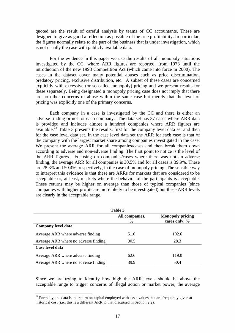
Each company in a case is investigated by the CC and there is either an adverse finding or not for each company. The data set has 37 cases where ARR data is provided and includes almost a hundred companies where ARR figures are available.24 Table 3 presents the results, first for the company level data set and then for the case level data set. In the case level data set the ARR for each case is that of the company with the largest market share among companies investigated in the case. We present the average ARR for all companies/cases and then break them down according to adverse and non-adverse finding. The first point to notice is the level of the ARR figures. Focusing on companies/cases where there was not an adverse finding, the average ARR for all companies is 30.5% and for all cases is 39.9%. These are 28.3% and 50.4%, respectively, in the case of monopoly pricing. The sensible way to interpret this evidence is that these are ARRs for markets that are considered to be acceptable or, at least, markets where the behavior of the participants is acceptable. These returns may be higher on average than those of typical companies (since companies with higher profits are more likely to be investigated) but these ARR levels are clearly in the acceptable range.

Table 3

All companies, %

Monopoly pricing cases only, %

Company level data

Average ARR where adverse finding 51.0 102.6 Average ARR where no adverse finding 30.5 28.3 Case level data

Average ARR where adverse finding 62.6 119.0 Average ARR where no adverse finding 39.9 50.4 Since we are trying to identify how high the ARR levels should be above the acceptable range to trigger concerns of illegal action or market power, the average

24 Formally, the data is the return on capital employed with asset values that are frequently given at historical cost (i.e., this is a different ARR to that discussed in Section 2.2).

17

ARRs for adverse findings and the difference between the adverse and non-adverse findings is also relevant. These differences range from 20.5% at the lowest (all companies, company level data set) to 74.3% at the highest (all companies, monopoly pricing cases, company level data set).

Summarizing, this evidence suggests that the difference between an ARR for a market without any adverse activity and those where the CC have decided to make an adverse finding is around 20% generally, and over 70% where the abuse has involved monopoly pricing. These are additions to what the CC perceives as acceptable ARRs, which themselves are in the order of 20% plus. This evidence provides strong confirmation of the general point made in this chapter, namely, that profitability measures need to be extremely high before they can be taken as reliable evidence of excessive pricing. 6. Summary and Conclusion

Section 2 of the paper has shown that in theory both IRR and ARR can be used to identify whether a company is earning an excess return. Although in the context of the ARR the necessary adjustments to asset values are not usually made, at least in theory, the ARR is able to identify excess returns and will be exactly equal to the IRR in some cases.

However, Section 3 of the paper highlights problems that arise when identifying a meaningful benchmark and argues that, for competition law purposes, profitability measures normally need to identify excessive profitability not excess profit. The inability to measure all assets and contract risks properly and the role of real options suggests that the difference between the cost of capital and an “excessive” level of profitability is likely to be significant. Furthermore, standard errors surrounding the estimation of the cost of capital contribute to this difference. Evidence from the U.K., one of the few jurisdictions to assess profitability systematically, suggests that the difference between a reasonable ARR for a market without any adverse activity and a market where the CC have decided to make an adverse finding may be around 20% generally and over 50% where the abuse has involved monopoly pricing.

Section 4 then shows that the IRR and ARR are less well equipped to calculate the extent of excessive profitability than excess returns. Examples are given that show that IRRs can change significantly as business practices change even when they do not impact on present value, and hence have no effect on how much is being taken out of the market.

We conclude that it is dangerous to simply calculate one number and take this as the measure of profitability. A single number may tell you that a company earns an excess return (i.e., above the cost of capital) but may provide a very misleading picture as to whether the company is earning an excessive return or not. The profitability figure may be the consequence of the particular way that the company does business and small changes to practices may change the outcome significantly. It is necessary to address what alternative arrangements would be possible and what

18

impact these would have on the IRR. For this reason significant judgment is needed to use profitability measures in competition law cases. In addition, profitability can only be one input into a more comprehensive analysis. Profitability measures are useful in competition law but the analysis is far more of an art form and far less of a statistical procedure than, say, deriving the cost of capital. Anyone who has estimated cost of capital figures for competition law cases will immediately realize how much judgment is therefore required to bring insight to whether profits are excessive or not. References: Michael F. van Breda, The Misuse of Accounting Rates of Return: Comment, 74 Am. Econ. Rev. 507-508 (1984). Thomas E. Copeland, and J. Fred Weston, Financial Theory and Corporate Policy (1998). Avinash K. Dixit, and Robert S. Pindyck, Investment Under Uncertainty (1994). Avinash K. Dixit, and Robert S. Pindyck, The Options Approach to Capital Investment, Harvard Business Rev. May Issue (1995). Jeremy Edwards, John Kay and Colin Mayer, The Economic Analysis of Accounting Profitability, (1987) Oxford: Clarendon Press. European Commission XXIV Report on Competition Policy (1994). European Commission, Case 26/75, General Motors v. Commission [1975] ECR 1376, [1976] 1 CMLR 95. European Commission Case 226/84, British Leyland v. EC Commission [1986] ECR 3263, [1987] 1 CMLR 185 European Court of Justice, Case 27/76 United Brands v. Commission [1978] ECR 207, [1978] 1 CMLR 429 Franklin M. Fisher, The Misuse of Accounting Rates of Return: Reply, 74 Am. Econ. Rev. 509-517 (1984). Franklin M. Fisher, Market Power, (2006 - this volume). Franklin M. Fisher, and John J. McGowan, On the Misuse of Accounting Rate of Return to Inter Monopoly Profits, 73 Am. Econ. Rev. 82-97 (1983). Eleanor M. Fox, Monopolization and Dominance in the United States and the European Community: Efficiency, Opportunity, and Fairness, 61 Notre Dame Law Rev. 981-1020 (1986). John R. Graham, and Campbell R. Harvey, The Theory and Practice of Corporate Finance: Evidence from the Field, 60 Journal of Fin. Econ. 187-243 (2001).

19

Paul A. Grout and Anna Zalewska, The Impact of Regulation on Market Risk, 80 Journal of Fin. Econ. 149-184 (2006). Ira Horowitz, The Misuse of Accounting Rates of Return: Comment, 74 Am. Econ. Rev. 492-493 (1984). Harold Hotelling, A General Mathematical Theory of Depreciation, 20 Journal of the Am. Stat. Assoc. 340-353 (1925). Barry E. Hawk, The American (Anti-trust) Revolution: Lessons for the EEC?, 9 European Comp. Law Rev. 53-87 (1988). Thomas E. Kauper, Whither Article 86? Observation on Excessive Prices and Refusal to Deal, in B. Hawk (ed) Fordham Corp. Law Inst. 651-686 (1990). William F. Long, and David J. Ravenscraft, The Misuse of Accounting Rates of Return: Comment, Am. Econ. Rev. 494-500 (1984). Stephen Martin, The Misuse of Accounting Rates of Return: Comment, 74 Am. Econ. Rev. 501-506 (1984). Sir Derek Morris, Dominant Firm Behaviour under UK Competition Law, paper presented to the Fordham Law Institute Thirtieth Annual Conference on International Antitrust Law and Policy (2003). Massimo Motta and Alexandre de Streel, Exploitative and Exclusionary Prices in EU Law, in Claus-Dieter Ehlermann and Isabela Atanasiu (eds) What Is an Abuse of a Dominant Position?, Oxford, Hart (2006). Office of Fair Trading, Assessing Profitability in Competition Policy Analysis, (July 2003). Office of Telecommunications Regulation, Effective Competition Review of the UK Mobile Industry, (February 2001). Robert S. Pindyck, Sunk Costs and Real Options in Antitrust, NBER Working Paper No 11430 (2005). Richard Whish, Competition Law (Butterworths: 4th Edition 2001)

20

Appendix

This appendix provides an illustration of the relationship between ARR, the cost of capital and net present value in a simple setting. The definition of the deprival value of an asset is:

⎪⎪

⎩

⎪⎪

⎨

⎧

⎪⎩

⎪⎨⎧

(NRV)ValueRealizableNet

(NPV)ValuePresentNetofmaximumthe

(RC)CosttReplacemen

ofminimumtheisvalueDeprival

The net present value can be defined as

.111 ρρ +

++−

=−ttt

tNPVCR

NPV (A1)

We now make a simplifying assumption that in equilibrium net realizable value cannot be more than replacement cost or net present value (the justification for the assumption being that it would in this case make sense to realize the value of the asset rather than hold on to it). Given this assumption we can rewrite Equation (3), using (A1), as:

,11 111 ρ

ρρ +

−+

+−

=− −−−t

ttt

ttARRAANPVANPV (A2)

where and are the deprival value of assets at time t - 1 and t respectively. 1−tA tA First, consider the case when . It is clear from Equation (A2) that if the ARR is greater than the cost of capital (i.e.,

tt ANPV >ρ>tARR ), then the right hand side of

Equation (A2) is positive which means that , i.e., . 11 −− > tt ANPV 11 −− > tt RCNPV The alternative case is if tt ANPV ≤ . Given the definition of deprival value and the simplifying assumption it follows that tt ANPV = . Again, if ARR is greater than the cost of capital then , i.e., . 11 −− > tt ANPV 11 −− > tt RCNPV Therefore, if assets are defined by deprival value it follows that if the ARR is greater than the cost of capital, then the NPV of the assets is greater than their replacement cost, i.e., there is an excess return.25

25 The ARR has been calculated over a segment, hence we talk of NPV being greater than replacement cost rather than NPV being positive. At will be zero when we consider a segment at the start of a project. In this case, we talk of NPV being positive making the discussion equivalent to the previous results for IRR.

21