Embed Size (px)
Citation preview

Epid 766 D. Zhang
EPID 766: Analysis of Longitudinal Datafrom Epidemiologic Studies
Daowen Zhang
http://www4.stat.ncsu.edu/∼dzhang2
Graduate Summer Session in Epidemiology Slide 1

TABLE OF CONTENTS Epid 766, D. Zhang
Contents
1 Review and introduction to longitudinal studies 5
1.1 Review of 3 study designs . . . . . . . . . . . . . . . . . . . 5
1.2 Introduction to longitudinal studies . . . . . . . . . . . . . . 11
1.3 Data examples . . . . . . . . . . . . . . . . . . . . . . . . . 12
1.4 Features of longitudinal data . . . . . . . . . . . . . . . . . 22
1.5 Why longitudinal studies? . . . . . . . . . . . . . . . . . . . 24
1.6 Challenges in analyzing longitudinal data . . . . . . . . . . . 27
1.7 Methods for analyzing longitudinal data . . . . . . . . . . . 32
1.8 Two-stage method for analyzing longitudinal data . . . . . . 33
1.9 Analyzing Framingham data using two-stage method . . . . 35
2 Linear mixed models for normal longitudinal data 50
2.1 What is a linear mixed (effects) model? . . . . . . . . . . . 51
2.2 Estimation and inference for linear mixed models . . . . . . 68
2.3 How to choose random effects and the error structure? . . . 70
Graduate Summer Session in Epidemiology Slide 2
TABLE OF CONTENTS Epid 766, D. Zhang
2.4 Analyze Framingham data using linear mixed models . . . . 71
2.5 GEE for linear mixed models . . . . . . . . . . . . . . . . . 1072.6 Missing data issues . . . . . . . . . . . . . . . . . . . . . . 111
3 Modeling and design issues 116
3.1 How to handle baseline response? . . . . . . . . . . . . . . . 117
3.2 Do we model previous responses as covariates? . . . . . . . 119
3.3 Modeling outcome vs. modeling the change of outcome . . . 121
3.4 Design a longitudinal study: Sample size estimation . . . . . 131
4 Modeling discrete longitudinal data 138
4.1 Generalized estimating equations (GEEs) for continuous anddiscrete longitudinal data . . . . . . . . . . . . . . . . . . . 139
4.1.1 Why GEEs? . . . . . . . . . . . . . . . . . . . . . . 139
4.1.2 Key features of GEEs for analyzing longitudinal data 143
4.1.3 Some popular GEE Models . . . . . . . . . . . . . . 145
4.1.4 Some basics of GEEs . . . . . . . . . . . . . . . . . 1474.1.5 Interpretation of regression coefficients in a GEE Model153
Graduate Summer Session in Epidemiology Slide 3

TABLE OF CONTENTS Epid 766, D. Zhang
4.1.6 Analyze Infectious disease data using GEE . . . . . . 155
4.1.7 Analyze epileptic seizure count data using GEE . . . 162
4.2 Generalized linear mixed models (GLMMs) . . . . . . . . . . 172
4.2.1 Model specification and implementation . . . . . . . 172
4.3 Analyze infectious disease data using a GLMM . . . . . . . . 183
4.4 Analyze epileptic count data using a GLMM . . . . . . . . . 194
5 Summary: what we covered 205
Graduate Summer Session in Epidemiology Slide 4

CHAPTER 1 Epid 766, D. Zhang
1 Review and introduction to longitudinal
studies
• Review of 3 study designs
• Introduction to longitudinal (panel) studies
• Data examples
• Features of longitudinal data
• Why longitudinal studies
• Challenges in analyzing longitudinal data
• Methods for analyzing longitudinal data: two-stage, linear mixed
model, GEE, transition models
• Two-stage method for analyzing longitudinal data
• Analyzing Framingham data using two-stage method
Graduate Summer Session in Epidemiology Slide 5

CHAPTER 1 Epid 766, D. Zhang
1.1 Review of 3 study designs
1. Cross-sectional study:
• Information on the disease status (Y ) and the exposure status (X)
is obtained from a random sample at one time point. A snap
shot of population.
• A single observation of each variable of interest is measured from
each subject: (Yi, Xi) (i = 1, ..., n). Regression such as logistic
regression (if Yi is binary) can be used to assess the association
between Y and X:
log
(P[Yi = 1|Xi]
1− P[Yi = 1|Xi]
)= β0 + β1Xi
β1 = log
(P[Y = 1|X = 1]/(1− P[Y = 1|X = 1])
P[Y = 1|X = 0]/(1− P[Y = 1|X = 0])
)β1 = log odds-ratio between exposure population (X = 1) and non
exposure population (X = 0). β1 > 0 =⇒ the exposure population
has a higher probability of getting the disease.Graduate Summer Session in Epidemiology Slide 6
CHAPTER 1 Epid 766, D. Zhang
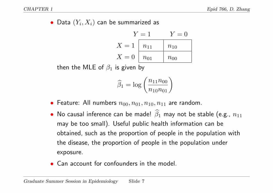
• Data (Yi, Xi) can be summarized as
Y = 1 Y = 0
X = 1 n11 n10
X = 0 n01 n00
then the MLE of β1 is given by
β1 = log
(n11n00n10n01
)• Feature: All numbers n00, n01, n10, n11 are random.
• No causal inference can be made! β1 may not be stable (e.g., n11
may be too small). Useful public health information can be
obtained, such as the proportion of people in the population with
the disease, the proportion of people in the population under
exposure.
• Can account for confounders in the model.
Graduate Summer Session in Epidemiology Slide 7

CHAPTER 1 Epid 766, D. Zhang
2. Prospective cohort study (follow-up study):
• A cohort with known exposure status (X) is followed over time to
obtain their disease status (Y ).
• A single observation of (Y ) may be observed (e.g., survival study)
or multiple observations of (Y ) may be observed (longitudinal
study).
• Stronger evidence for causal inference. Causal inference can be
made if X is assigned randomly (if X is a treatment indicator in
the case of clinical trials).
• When single binary (0/1) Y is obtained, we have
D D
E n11 n10 n1+
E n01 n00 n0+
Here, n1+ and n0+ are fixed (sample sizes for the exposure and
non-exposure groups).
Graduate Summer Session in Epidemiology Slide 8

CHAPTER 1 Epid 766, D. Zhang
3. Retrospective (case-control) study:
• A sample with known disease status (D) is drawn and their
exposure history (E) is ascertained. Data can be summarized as
D D
E n11 n10
E n01 n00
n+1 n+0
where the margins n+1 and n+0 are fixed numbers.
• Assuming no bias in obtaining history information on E, association
between E and D can be estimated.
n11 ∼ Bin(n+1, P [E|D]), n10 ∼ Bin(n+0, P [E|D]).
Odds ratio: estimate from this study
θ =n11n00n10n01
Graduate Summer Session in Epidemiology Slide 9

CHAPTER 1 Epid 766, D. Zhang
estimates the following quantity
θ =P [E|D]/(1− P [E|D])
P [E|D]/(1− P [E|D])=P [D|E]/(1− P [D|E])
P [D|E]/(1− P [D|E]).
• If disease is rare, i.e., P [D|E] ≈ 0, P [D|E] ≈ 0, relative risk of
disease can be approximately obtained:
θ ≈ P [D|E]
P [D|E]= relative risk.
More efficient than prospective cohort study in this case.
• Problem: recall bias! (it is difficult to ascertain exposure history
E.)
Graduate Summer Session in Epidemiology Slide 10
CHAPTER 1 Epid 766, D. Zhang
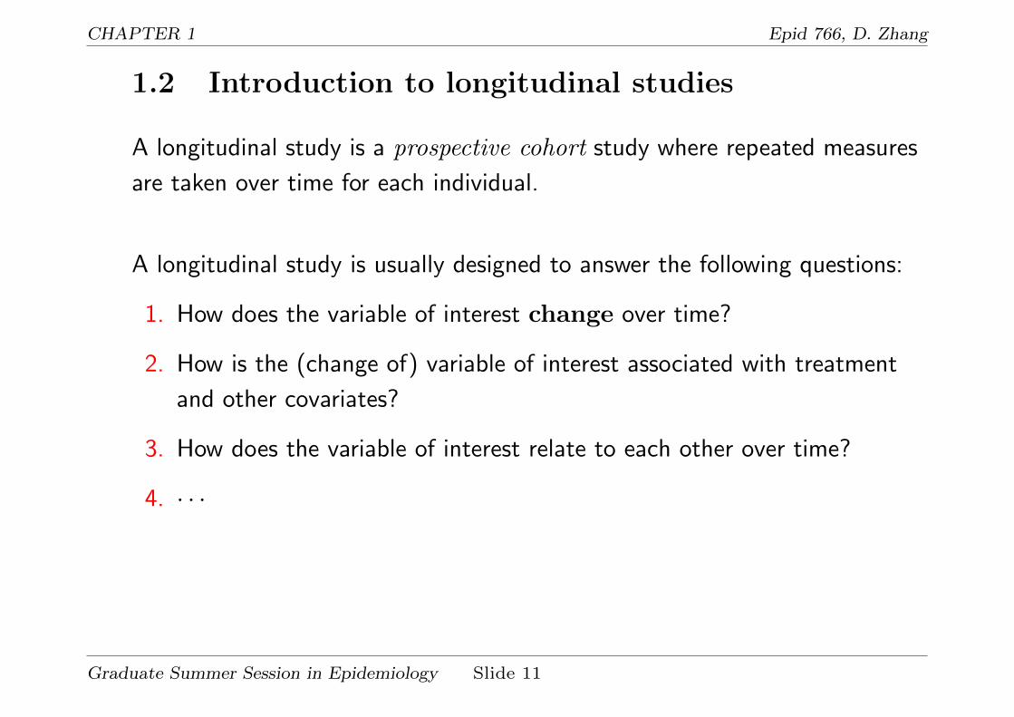
1.2 Introduction to longitudinal studies
A longitudinal study is a prospective cohort study where repeated measures
are taken over time for each individual.
A longitudinal study is usually designed to answer the following questions:
1. How does the variable of interest change over time?
2. How is the (change of) variable of interest associated with treatment
and other covariates?
3. How does the variable of interest relate to each other over time?
4. · · ·
Graduate Summer Session in Epidemiology Slide 11
CHAPTER 1 Epid 766, D. Zhang
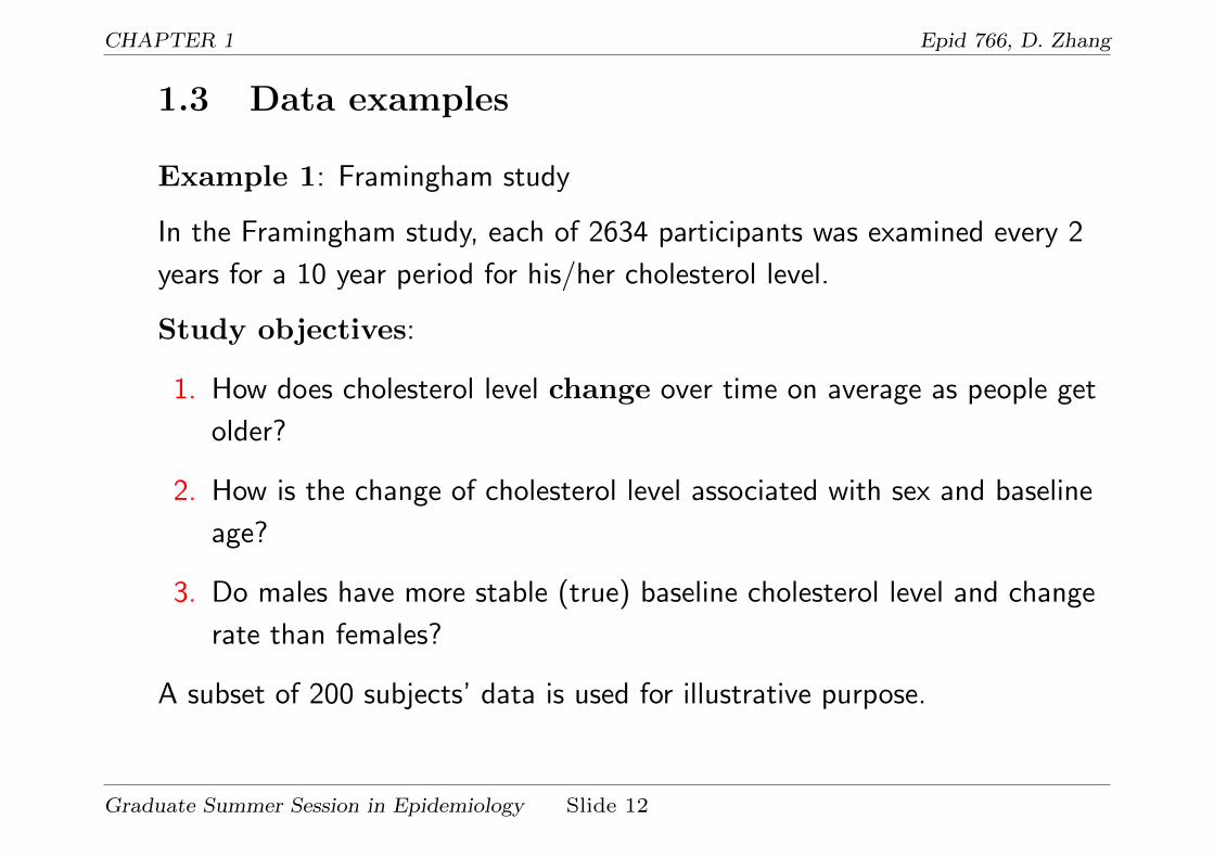
1.3 Data examples
Example 1: Framingham study
In the Framingham study, each of 2634 participants was examined every 2
years for a 10 year period for his/her cholesterol level.
Study objectives:
1. How does cholesterol level change over time on average as people get
older?
2. How is the change of cholesterol level associated with sex and baseline
age?
3. Do males have more stable (true) baseline cholesterol level and change
rate than females?
A subset of 200 subjects’ data is used for illustrative purpose.
Graduate Summer Session in Epidemiology Slide 12

CHAPTER 1 Epid 766, D. Zhang
A glimpse of the raw data
newid id cholst sex age time
1 1244 175 1 32 0
1 1244 198 1 32 2
1 1244 205 1 32 4
1 1244 228 1 32 6
1 1244 214 1 32 8
1 1244 214 1 32 10
2 835 299 0 34 0
2 835 328 0 34 4
2 835 374 0 34 6
2 835 362 0 34 8
2 835 370 0 34 10
3 176 250 0 41 0
3 176 277 0 41 2
3 176 265 0 41 4
3 176 254 0 41 6
3 176 263 0 41 8
3 176 268 0 41 10
4 901 243 0 44 0
4 901 211 0 44 2
4 901 204 0 44 4
4 901 196 0 44 6
4 901 246 0 44 8
Graduate Summer Session in Epidemiology Slide 13

CHAPTER 1 Epid 766, D. Zhang
Cholesterol level over time for a subset of 200 subjects from
Framingham study
Graduate Summer Session in Epidemiology Slide 14

CHAPTER 1 Epid 766, D. Zhang
What we observed from this data set:
1. Cholesterol levels increase (linearly) over time for most individuals.
2. Each subject has his/her own trajectory line with a possibly different
intercept and slope, implying two sources of variations: within and
between subject variations.
3. Each subject has on average 5 observations (as opposed to one
observation per subject for a cross-sectional study)
4. The data is not balanced. Some individuals have missing observations
(e.g., subject 2’s Cholesterol is missing at time = 2)
5. The inference is NOT limited to these 200 individuals. Instead, the
inference is for the target population and each subject is viewed as a
random person drawn from the target population.
Graduate Summer Session in Epidemiology Slide 15
CHAPTER 1 Epid 766, D. Zhang
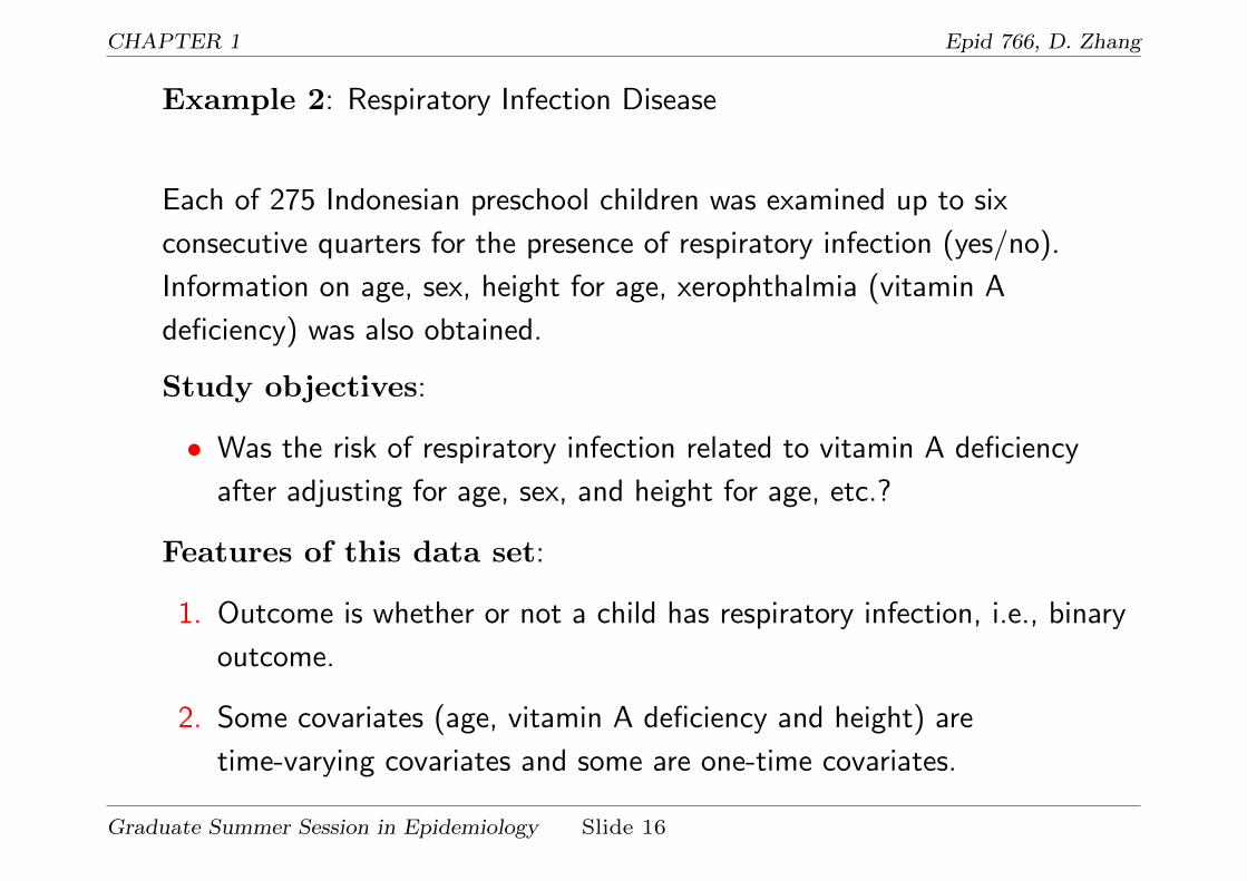
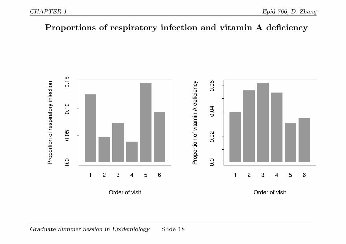
Example 2: Respiratory Infection Disease
Each of 275 Indonesian preschool children was examined up to six
consecutive quarters for the presence of respiratory infection (yes/no).
Information on age, sex, height for age, xerophthalmia (vitamin A
deficiency) was also obtained.
Study objectives:
• Was the risk of respiratory infection related to vitamin A deficiency
after adjusting for age, sex, and height for age, etc.?
Features of this data set:
1. Outcome is whether or not a child has respiratory infection, i.e., binary
outcome.
2. Some covariates (age, vitamin A deficiency and height) are
time-varying covariates and some are one-time covariates.
Graduate Summer Session in Epidemiology Slide 16

CHAPTER 1 Epid 766, D. Zhang
A glimpse of the infection data
Print the first 20 observations 1
Obs id infect xero sex visit season
1 121013 0 0 0 1 2
2 121013 0 0 0 2 3
3 121013 0 0 0 3 4
4 121013 0 0 0 4 1
5 121013 1 0 0 5 2
6 121013 0 0 0 6 3
7 121113 0 0 1 1 2
8 121113 0 0 1 2 3
9 121113 0 0 1 3 4
10 121113 0 0 1 4 1
11 121113 1 0 1 5 2
12 121113 0 0 1 6 3
13 121114 0 0 0 1 2
14 121114 0 0 0 2 3
15 121114 0 0 0 3 4
16 121114 1 0 0 4 1
17 121114 1 0 0 5 2
18 121114 0 0 0 6 3
19 121140 0 0 1 1 2
20 121140 0 1 1 2 3
Graduate Summer Session in Epidemiology Slide 17
CHAPTER 1 Epid 766, D. Zhang
Proportions of respiratory infection and vitamin A deficiency
Graduate Summer Session in Epidemiology Slide 18

CHAPTER 1 Epid 766, D. Zhang
Example 3: Epileptic seizure counts from the progabide trial
In the progabide trial, 59 epileptics were randomly assigned to receive the
anti-epileptic treatment (progabide) or placebo. The number of seizure
counts was recorded in 4 consecutive 2-week intervals. Age and baseline
seizure counts (in an eight week period prior to the treatment assignment)
were also recorded.
Study objectives:
• Does the treatment work?
• What is the treatment effect adjusting for available covariates?
Features of this data set:
1. Outcome is count data, implying a Poisson regression.
2. Baseline seizure counts were for 8 weeks, as opposed to 2 weeks for
other seizure counts.
3. Randomization may be taken into account in the data analysis.
Graduate Summer Session in Epidemiology Slide 19

CHAPTER 1 Epid 766, D. Zhang
A glimpse of the seizure data
Print the first 20 observations 1
Obs id seize trt visit interval age
1 101 76 1 0 8 18
2 101 11 1 1 2 18
3 101 14 1 2 2 18
4 101 9 1 3 2 18
5 101 8 1 4 2 18
6 102 38 1 0 8 32
7 102 8 1 1 2 32
8 102 7 1 2 2 32
9 102 9 1 3 2 32
10 102 4 1 4 2 32
11 103 19 1 0 8 20
12 103 0 1 1 2 20
13 103 4 1 2 2 20
14 103 3 1 3 2 20
15 103 0 1 4 2 20
16 104 11 0 0 8 31
17 104 5 0 1 2 31
18 104 3 0 2 2 31
19 104 3 0 3 2 31
20 104 3 0 4 2 31
Graduate Summer Session in Epidemiology Slide 20

CHAPTER 1 Epid 766, D. Zhang
Epileptic seizure counts from the progabide trial
Graduate Summer Session in Epidemiology Slide 21

CHAPTER 1 Epid 766, D. Zhang
1.4 Features of longitudinal data
Common features of all examples:
• Each subject has multiple time-ordered observations of response.
• Responses from the same subjects may be “more alike” than others.
• Inference is NOT in study subjects, but in population from which they
are from.
• # of subjects >> # of observations/subject
• Source of variations – between and within subject variations.
Difference in the examples:
• Different types of responses (continuous, binary, count).
• Objectives depend on the type of study – “mean” behavior, etc.
Graduate Summer Session in Epidemiology Slide 22

CHAPTER 1 Epid 766, D. Zhang
Comparison of data structures:
Classical study Longitudinal study
Subject Data Subject Data Time
1 x1 1 x11, x12, ..., x15 t11, t12, ..., t15
y1 y11, y12, ..., y15 t11, t12, ..., t15
2 x2 2 x21, x22, ..., x25 t21, t22, ..., t25
y2 y21, y22, ..., y25 t21, t22, ..., t25
For simplicity, we consider one covariate case.
Graduate Summer Session in Epidemiology Slide 23

CHAPTER 1 Epid 766, D. Zhang
1.5 Why longitudinal studies?
1. A longitudinal study allows us to study the change of the variable of
interest over time, either at population level or individual level.
2. A longitudinal study enables us to separately estimate the
cross-sectional effect (e.g., cohort effect) and the longitudinal effect
(e.g., aging effect):
Given yij , ageij (j = 1, 2, · · · , ni, j = 1 is the baseline). In a
cross-sectional study, ni = 1 and we are forced to fit the following
model
yi1 = β0 + βCagei1 + εi1.
That is, βC is the cross-sectional effect of age.
With longitudinal data (ni > 1), we can entertain the model
yij = β0 + βCagei1 + βL(ageij − agei1) + εij .
Graduate Summer Session in Epidemiology Slide 24

CHAPTER 1 Epid 766, D. Zhang
Then
yi1 = β0 + βCagei1 + εi1 (let j = 1),
yij − yi1 = βL(ageij − agei1) + εij − εi1.
That is, βL is the longitudinal effect of age and in general βL 6= βC .
3. A longitudinal study is more powerful to detect an association of
interest compared to a cross-sectional study, =⇒ more efficient, less
sample size (number of subjects).
4. A longitudinal study allows us to study the within-subject and
between-subject variations.
Suppose b ∼ (µ, σ2b ) is the blood pressure for a patient population.
However, what we observe is Y = b+ ε, where ε ∼ (0, σ2ε) is the
measurement error.
• σ2ε = within-subject variation
• σ2b = between-subject variation
Graduate Summer Session in Epidemiology Slide 25

CHAPTER 1 Epid 766, D. Zhang
If we have only one observation Yi for each subject from a sample of n
patients, then we can’t separate σ2ε and σ2
b . Although we can use data
Y1, Y2, ..., Yn to make inference on µ, we can’t make any inference on
σ2b .
However, if we have repeated (or longitudinal) measurements Yij of
blood pressure for each subjects, then
Yij = bi + εij .
Now, it is possible to make inference about all quantities µ, σ2b and σ2
ε .
5. A longitudinal study provides more evidence for possible causal
interpretation.
Graduate Summer Session in Epidemiology Slide 26

CHAPTER 1 Epid 766, D. Zhang
1.6 Challenges in analyzing longitudinal data
Key assumptions in a classical regression model: There is only
one observation of response per subject, =⇒ responses are independent to
each other. For example, when y = cholesterol level,
yi = β0 + β1sexi + β2agei + εi.
However, the observations from the same subject in a longitudinal study
tend to be more similar to each other than those observations from other
subjects, =⇒ responses (from the same subjects) are not independent any
more. Although, the observations from different subjects are still
independent.
What happens if we treat observations as independent (i.e.,
ignore the correlation)?
1. In general, the estimation of the associations (regression coefficients)
of the outcome and covariates is valid.
Graduate Summer Session in Epidemiology Slide 27
CHAPTER 1 Epid 766, D. Zhang
2. However, the variability measures (e.g, the SEs from a classical
regression analysis) are not right: sometimes smaller, sometimes bigger
than the true variability.
3. Therefore, the inference is not valid (too significant than it should be if
the SE is too small).
Sources of variation and correlation in longitudinal data:
1. Between-subject variation: For the blood pressure example, if each
subject’s blood pressures were measured within a relatively short time,
then the following model may be a reasonable one:
yij = bi + εij ,
where bi is the true blood pressure of subject i with variance σ2b , εij is
the independent (random) measurement error with variance σ2ε ,
independent of bi.
Graduate Summer Session in Epidemiology Slide 28

CHAPTER 1 Epid 766, D. Zhang
For j 6= k,
corr(yij , yik) =cov(yij , yik)√
var(yij)var(yik)
=σ2b
σ2b + σ2
ε
.
Therefore, if the between-subject variation σ2b 6= 0, then data from the
same subjects are correlated.
Graduate Summer Session in Epidemiology Slide 29

CHAPTER 1 Epid 766, D. Zhang
The blood pressure example
Graduate Summer Session in Epidemiology Slide 30
CHAPTER 1 Epid 766, D. Zhang
2. Serial correlation: If the time intervals between blood pressure
measurements are relatively large so it may not be reasonable to
assume a constant blood pressure for each subject:
yij = bi + Ui(tij) + εij ,
where bi = true long-term blood pressure, Ui(tij) =a stochastic
process (like a time series) due to biological fluctuation of blood
pressure, εij is the independent (random) measurement error. Here the
correlation is caused by both bi and Ui(tij).
3. In a typical longitudinal study for human where # of
observations/subject is small to moderate, there may not be enough
information for the serial correlation and most correlation can be
accounted for by (possibly complicated) between-subject variation.
Graduate Summer Session in Epidemiology Slide 31

CHAPTER 1 Epid 766, D. Zhang
1.7 Methods for analyzing longitudinal data
1. Two-stage: summarize each subject’s outcome and regress the
summary statistics on one-time covariates. Especially useful for
continuous longitudinal data. However, this method is getting
out-dated since the mixed model approach can do the same thing even
better.
2. Mixed (effects) model approach: model fixed effects and random
effects; use random effects to model correlation.
3. Generalized estimating equation (GEE) approach: model the
dependence of marginal mean on covariates. Correlation is not a main
interest. Particularly good for discrete data.
4. Transition models: use history as covariates. Good for prediction of
future response using history.
Graduate Summer Session in Epidemiology Slide 32

CHAPTER 1 Epid 766, D. Zhang
1.8 Two-stage method for analyzing longitudinal
data
• Outcome (usually continuous): yi1, ..., yinimeasured at ti1, ..., tini
;
one-time covariates: xi1, ..., xip.
• Two-stage analysis is conducted as follows:
1. Stage 1: Get summary statistics from subject i’s data: yi1, ..., yini .
For example, use mean yi = (yi1 + · · ·+ yini)/ni or fit a linear
regression for each subject:
yij = bi0 + bi1tij + εij ,
and get estimates bi0, bi1 of bi0 and bi1. Here we assume that
subject i’s true response at time tij is given by
bi0 + bi1tij ,
a straight line. Suppose t = 0 is the baseline, then bi0 is subject i’s
true response at baseline and bi1 is subject i’s change rate of the
Graduate Summer Session in Epidemiology Slide 33

CHAPTER 1 Epid 766, D. Zhang
true response (not y). The error term εij can be regarded as
measurement error.
2. Stage 2: Treat the summary statistics as new responses and regress
the summary statistics on one-time covariates. For example, after
we got bi0 and bi1, we can calculate the means of bi0 and bi1 and
the standard errors of those means, compare bi0, bi0 among
genders, or do the following regressions
bi0 = α0 + α1xi1 + · · ·+ αpxip + ei0
bi1 = β0 + β1xi1 + · · ·+ βpxip + ei1.
Here, αk is the effect of xk on the true baseline response (not y),
βk is the effect of xk on the change rate of of the true response.
Graduate Summer Session in Epidemiology Slide 34
CHAPTER 1 Epid 766, D. Zhang
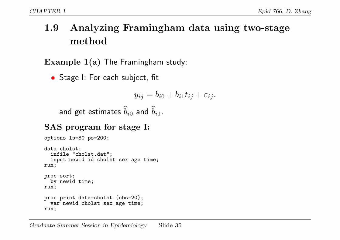
1.9 Analyzing Framingham data using two-stage
method
Example 1(a) The Framingham study:
• Stage I: For each subject, fit
yij = bi0 + bi1tij + εij .
and get estimates bi0 and bi1.
SAS program for stage I:options ls=80 ps=200;
data cholst;infile "cholst.dat";input newid id cholst sex age time;
run;
proc sort;by newid time;
run;
proc print data=cholst (obs=20);var newid cholst sex age time;
run;
Graduate Summer Session in Epidemiology Slide 35

CHAPTER 1 Epid 766, D. Zhang
title "First stage in two-stage analysis";proc reg outest=out noprint;
model cholst = time;by newid;
run;
data out; set out;b0hat = intercept;b1hat = time;keep newid b0hat b1hat;
run;
data main; merge cholst out;by newid;if first.newid=1;
run;
title "Summary statistics for intercepts and slopes";proc means mean stderr var t probt;
var b0hat b1hat;run;
title "Correlation between intercepts and slopes";proc corr;var b0hat b1hat;
run;
Graduate Summer Session in Epidemiology Slide 36
CHAPTER 1 Epid 766, D. Zhang
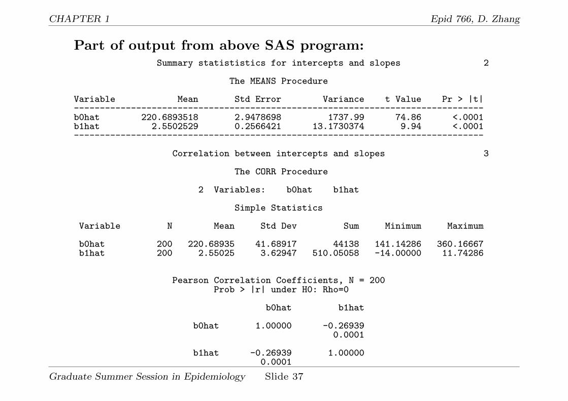
Part of output from above SAS program:Summary statististics for intercepts and slopes 2
The MEANS Procedure
Variable Mean Std Error Variance t Value Pr > |t|-------------------------------------------------------------------------------b0hat 220.6893518 2.9478698 1737.99 74.86 <.0001b1hat 2.5502529 0.2566421 13.1730374 9.94 <.0001-------------------------------------------------------------------------------
Correlation between intercepts and slopes 3
The CORR Procedure
2 Variables: b0hat b1hat
Simple Statistics
Variable N Mean Std Dev Sum Minimum Maximum
b0hat 200 220.68935 41.68917 44138 141.14286 360.16667b1hat 200 2.55025 3.62947 510.05058 -14.00000 11.74286
Pearson Correlation Coefficients, N = 200Prob > |r| under H0: Rho=0
b0hat b1hat
b0hat 1.00000 -0.269390.0001
b1hat -0.26939 1.000000.0001
Graduate Summer Session in Epidemiology Slide 37

CHAPTER 1 Epid 766, D. Zhang
Summary statistics from stage 1:
Parameter mean SE t P [T ≥ |t|]
b0 221 3 75 < .0001
b1 2.55 0.257 10 < .0001 corr(b0, b1) = −0.27
S2b0
= 1738, S2b1
= 13.2.
Note:
1. Similar to the blood pressure example, we can use the sample means of
b0 and b1 to estimate the means of b0 and b1. Hence we can use
sample mean of b1 (2.55) and its SE (0.257) to answer the first
objective of this study.
2. However, since var(bi0) and var(bi1) contain variability due to
estimating the true baseline response bi0 and change rate bi1 for
individual i, so
var(bi0) > var(bi0), var(bi1) > var(bi1).
Graduate Summer Session in Epidemiology Slide 38

CHAPTER 1 Epid 766, D. Zhang
Sample variances S2b0
and S2b1
are unbiased estimates of var(bi0) and
var(bi1) and would overestimate var(bi0) and var(bi1).
3. Similarly,
corr(b0, b1) 6= corr(b0, b1).
Therefore, corr(b0, b1) = −0.27 cannot be used to estimate the
correlation between the true baseline response b0 and true change rate
b1.
4. We will use mixed model approach to address the above issues later.
Graduate Summer Session in Epidemiology Slide 39

CHAPTER 1 Epid 766, D. Zhang
• Stage II:
1. Try to compare E(b0) and E(b1) between males and females.
2. Try to compare var(b0) and var(b1) between males and females.
3. Try to examine the effects of age and sex on b0 using
b0 = α0 + α1sex + α2age + e0.
Technically, we should use b0 instead of b0. However, b0 is an
unbiased estimate of b0 (and b0 is not observable), so using b0 is
valid.
4. Try to examine the effects of age and sex on b1 using
b1 = β0 + β1sex + β2age + e1.
Similar to the above argument, using b1 here is valid.
Graduate Summer Session in Epidemiology Slide 40

CHAPTER 1 Epid 766, D. Zhang
SAS program for stage II:
title "Test equality of mean and variance of intercepts and slopes between sexes";proc ttest;
class sex;var b0hat b1hat;
run;
title "Regression to look at the association between intercept and sex, age";proc reg data=main;
model b0hat = sex age;run;
title "Regression to look at the association between slope and sex, age";proc reg data=main;
model b1hat = sex age;run;
Graduate Summer Session in Epidemiology Slide 41

CHAPTER 1 Epid 766, D. Zhang
Part of output from above SAS program:
Test equality of mean and variance of intercepts and slopes between sexes 4
The TTEST Procedure
Variable: b0hat
sex N Mean Std Dev Std Err Minimum Maximum
0 97 224.0 40.2259 4.0843 146.3 348.11 103 217.6 42.9885 4.2358 141.1 360.2Diff (1-2) 6.3629 41.6719 5.8960
sex Method Mean 95% CL Mean Std Dev 95% CL Std Dev
0 224.0 215.9 232.1 40.2259 35.2522 46.84651 217.6 209.2 226.0 42.9885 37.8123 49.8197Diff (1-2) Pooled 6.3629 -5.2640 17.9898 41.6719 37.9405 46.2237Diff (1-2) Satterthwaite 6.3629 -5.2408 17.9666
Method Variances DF t Value Pr > |t|
Pooled Equal 198 1.08 0.2818Satterthwaite Unequal 197.99 1.08 0.2809
Equality of Variances
Method Num DF Den DF F Value Pr > F
Folded F 102 96 1.14 0.5117
Graduate Summer Session in Epidemiology Slide 42
CHAPTER 1 Epid 766, D. Zhang
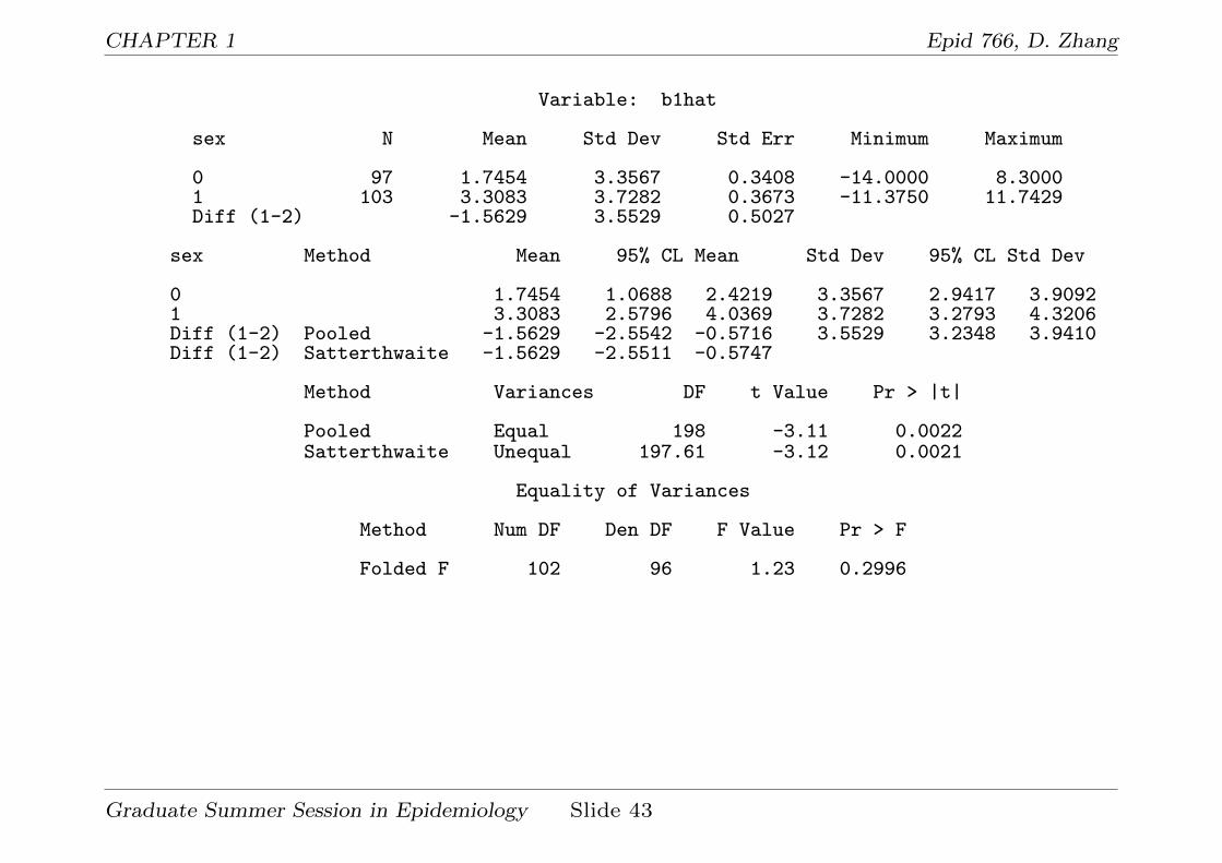
Variable: b1hat
sex N Mean Std Dev Std Err Minimum Maximum
0 97 1.7454 3.3567 0.3408 -14.0000 8.30001 103 3.3083 3.7282 0.3673 -11.3750 11.7429Diff (1-2) -1.5629 3.5529 0.5027
sex Method Mean 95% CL Mean Std Dev 95% CL Std Dev
0 1.7454 1.0688 2.4219 3.3567 2.9417 3.90921 3.3083 2.5796 4.0369 3.7282 3.2793 4.3206Diff (1-2) Pooled -1.5629 -2.5542 -0.5716 3.5529 3.2348 3.9410Diff (1-2) Satterthwaite -1.5629 -2.5511 -0.5747
Method Variances DF t Value Pr > |t|
Pooled Equal 198 -3.11 0.0022Satterthwaite Unequal 197.61 -3.12 0.0021
Equality of Variances
Method Num DF Den DF F Value Pr > F
Folded F 102 96 1.23 0.2996
Graduate Summer Session in Epidemiology Slide 43

CHAPTER 1 Epid 766, D. Zhang
Regression to look at the association between intercept and sex, age 5
The REG ProcedureModel: MODEL1
Dependent Variable: b0hat
Analysis of Variance
Sum of MeanSource DF Squares Square F Value Pr > F
Model 2 53715 26857 18.11 <.0001Error 197 292145 1482.96718Corrected Total 199 345859
Root MSE 38.50931 R-Square 0.1553Dependent Mean 220.68935 Adj R-Sq 0.1467Coeff Var 17.44956
Parameter Estimates
Parameter StandardVariable DF Estimate Error t Value Pr > |t|
Intercept 1 138.21793 15.04083 9.19 <.0001sex 1 -9.75053 5.47862 -1.78 0.0767age 1 2.05576 0.34820 5.90 <.0001
Graduate Summer Session in Epidemiology Slide 44
CHAPTER 1 Epid 766, D. Zhang
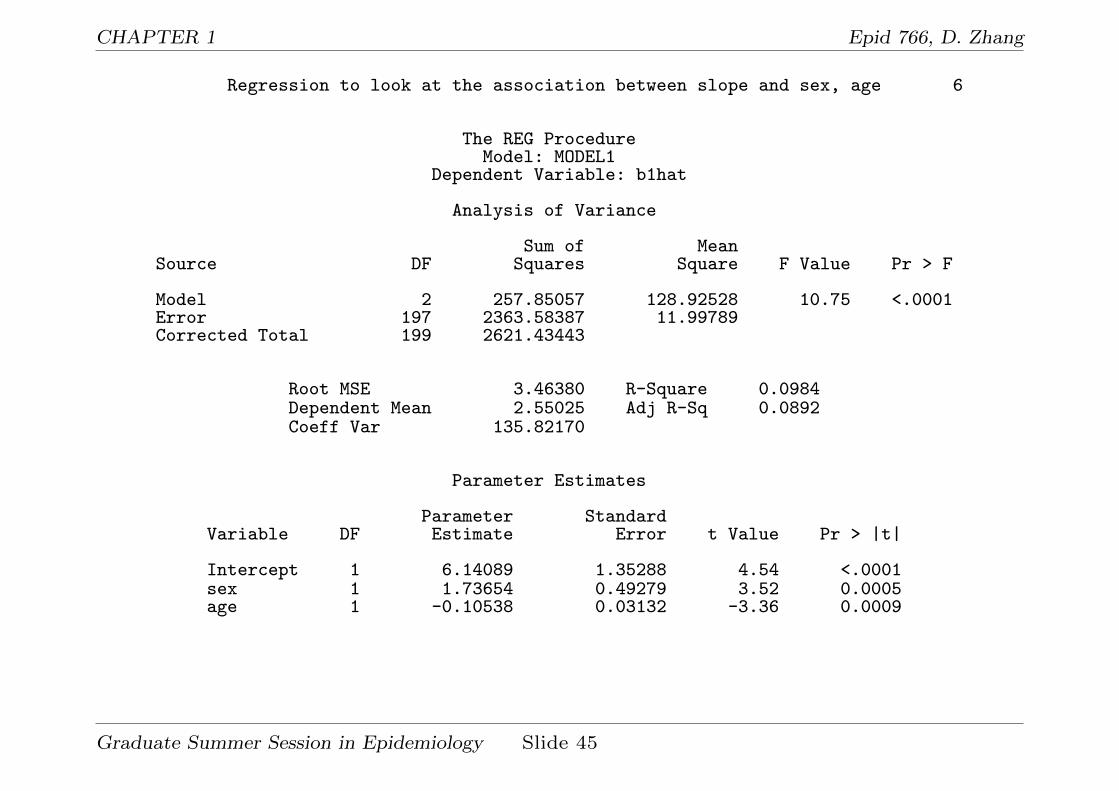
Regression to look at the association between slope and sex, age 6
The REG ProcedureModel: MODEL1
Dependent Variable: b1hat
Analysis of Variance
Sum of MeanSource DF Squares Square F Value Pr > F
Model 2 257.85057 128.92528 10.75 <.0001Error 197 2363.58387 11.99789Corrected Total 199 2621.43443
Root MSE 3.46380 R-Square 0.0984Dependent Mean 2.55025 Adj R-Sq 0.0892Coeff Var 135.82170
Parameter Estimates
Parameter StandardVariable DF Estimate Error t Value Pr > |t|
Intercept 1 6.14089 1.35288 4.54 <.0001sex 1 1.73654 0.49279 3.52 0.0005age 1 -0.10538 0.03132 -3.36 0.0009
Graduate Summer Session in Epidemiology Slide 45
CHAPTER 1 Epid 766, D. Zhang
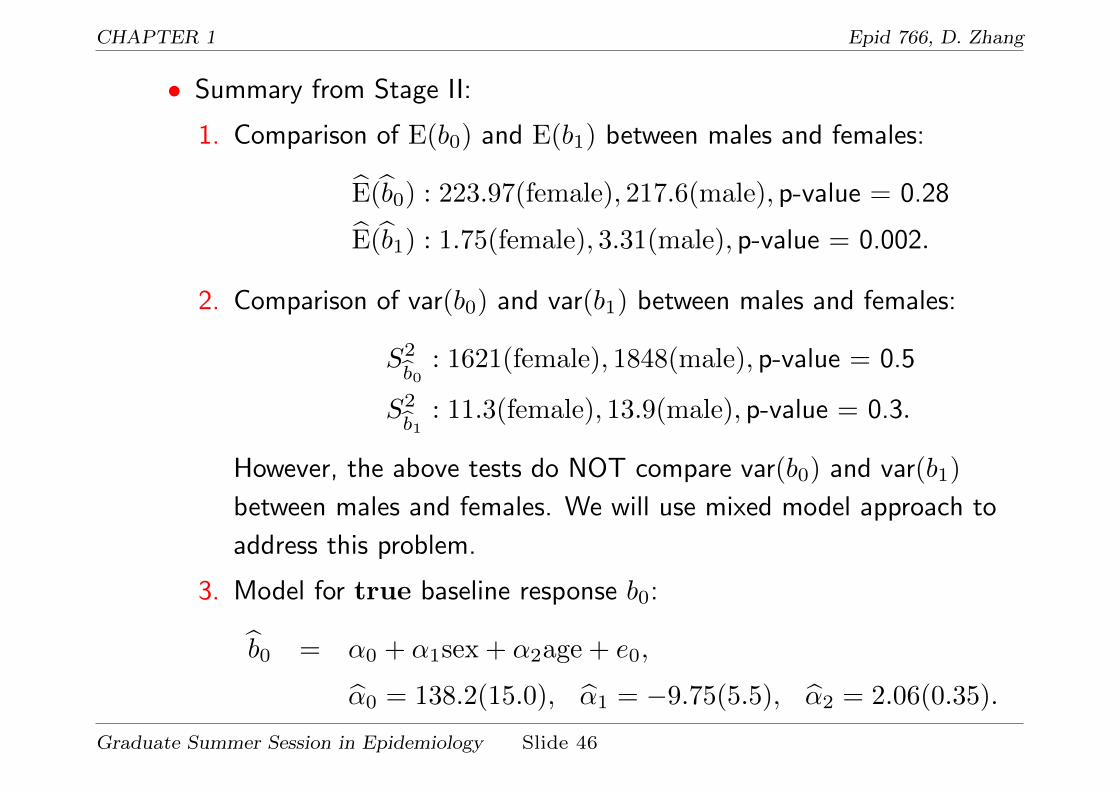
• Summary from Stage II:
1. Comparison of E(b0) and E(b1) between males and females:
E(b0) : 223.97(female), 217.6(male), p-value = 0.28
E(b1) : 1.75(female), 3.31(male), p-value = 0.002.
2. Comparison of var(b0) and var(b1) between males and females:
S2b0
: 1621(female), 1848(male), p-value = 0.5
S2b1
: 11.3(female), 13.9(male), p-value = 0.3.
However, the above tests do NOT compare var(b0) and var(b1)
between males and females. We will use mixed model approach to
address this problem.
3. Model for true baseline response b0:
b0 = α0 + α1sex + α2age + e0,
α0 = 138.2(15.0), α1 = −9.75(5.5), α2 = 2.06(0.35).
Graduate Summer Session in Epidemiology Slide 46

CHAPTER 1 Epid 766, D. Zhang
After adjusting for sex, one year increase in age corresponds to 2
unit increase in baseline cholesterol level. After adjusting for
baseline age, on average males’ baseline cholesterol level is about
10 units less than females’.
4. Model for change rate of the true response b1:
b1 = β0 + β1sex + β2age + e1,
β0 = 6.14(1.35), β1 = 1.74(0.5), β2 = −0.11(0.03).
After adjusting for sex, one year increase in age corresponds to 0.11
less in cholesterol level change rate. After adjusting for baseline age,
males’ cholesterol level change rate is 1.74 greater than females’.
Graduate Summer Session in Epidemiology Slide 47
CHAPTER 1 Epid 766, D. Zhang
Some remarks on two-stage analysis:
1. The first stage model should be reasonably good for the second stage
analysis to be valid and make sense.
2. Two-stage analysis can only be used when the covariates considered
are one-time covariates (fixed over time).
3. Summary statistics of a time-varying covariates cannot be used in the
second stage analysis because of error in variable issue.
4. When the covariates considered are time-varying covariates, two-stage
analysis is not appropriate. Mixed effects modeling or GEE approach
can be used.
5. Two-stage analysis can be applied to discrete response (binary or count
data). However, mixed effect modeling or GEE approach can be more
flexible.
6. Although two-stage approach can be used to make inference on the
quantities of interest, it is less efficient compared to the mixed model
Graduate Summer Session in Epidemiology Slide 48

CHAPTER 1 Epid 766, D. Zhang
approach. Therefore, mixed model approach should be used whenever
possible.
Graduate Summer Session in Epidemiology Slide 49

CHAPTER 2 Epid 766, D. Zhang
2 Linear mixed models for normal
longitudinal data
• What is a linear mixed model?
1. Random intercept model
2. Random intercept and slope model
3. Other error structures
4. General mixed models
• Estimation and inference
• Choose a variance matrix of the data
• Analyze Framingham data using linear mixed models
• GEE for mixed models, missing data issue
Graduate Summer Session in Epidemiology Slide 50
CHAPTER 2 Epid 766, D. Zhang
2.1 What is a linear mixed (effects) model?
A linear mixed model is an extension of a linear regression model to model
longitudinal (correlated) data. It contains fixed effects and random effects
where random effects are subject-specific and are used to model
between-subject variation and the correlation induced by this variation.
What are fixed effects? Fixed effects are the covariate effects that are
fixed across subjects in the study sample. These effects are the ones of our
particular interest. E.g., the regression coefficients in usual regression
models are fixed effects:
y = α+ xβ + ε.
What are random effects? Random effects are the covariate effects
that vary among subjects. So these effects are subject-specific and hence
are random (unobservable) since each subject is a random subject drawn
from a population.
Graduate Summer Session in Epidemiology Slide 51

CHAPTER 2 Epid 766, D. Zhang
I. Random intercept only model:
Data from m subjects:
Subject Outcome Time Random
intercept
1 y11, y12, ..., y1n1 t11, t12, ..., t1n1 b1
2 y21, y22, ..., y2n2t21, t22, ..., t2n2
b2
· · ·i yi1, yi2, ..., yini ti1, ti2, ..., tini bi
· · ·m ym1, ym2, ..., ymnm
tm1, tm2, ..., tmnmbm
Other covariates: xij2, ..., xijp, i = 1, ...,m, j = 1, ..., ni.
A random intercept model assumes:
yij = β0 + β1tij + β2xij2 + · · ·+ βpxijp + bi + εij .
Graduate Summer Session in Epidemiology Slide 52

CHAPTER 2 Epid 766, D. Zhang
Random intercept model:
yij = β0 + β1tij + β2xij2 + · · ·+ βpxijp + bi + εij
where β’s are fixed effects of interest, bi ∼ N(0, σ2b ) are random effects,
εij ∼ N(0, σ2ε) are independent (measurement)errors.
Interpretation of the model components:
1. From model,
E[yij ] = β0 + β1tij + β2xij2 + · · ·+ βpxijp.
2. βk: Average increase in y associated with one unit increase in xk, the
kth covariate, while others are held fixed.
3. β0 + β1tij + β2xij2 + · · ·+ βpxijp + bi = true response for subject i at
tij .
4. β0 + bi is the intercept for subject i =⇒ bi = deviation of intercept of
subject i from population intercept β0.
Graduate Summer Session in Epidemiology Slide 53

CHAPTER 2 Epid 766, D. Zhang
5. σ2b = between-subject variance, σ2
ε = within-subject variance.
6. Total variance of y: Var(yij) = σ2b + σ2
ε , constant over time.
7. Correlation between yij and yij′ :
corr(yij , yij′) =σ2b
σ2b + σ2
ε
= ρ
8. Correlation is constant and positive.
Graduate Summer Session in Epidemiology Slide 54

CHAPTER 2 Epid 766, D. Zhang
Why treat bi as random
1. Treating bi as random enables us to make inference for the whole
population from which the sample was drawn. Treating bi as fixed
would only allow us to make inference for the study sample.
2. Usually ni is small for longitudinal studies. Therefore, as the number
of total data points gets larger, the number of bi (which is m, the
number of subjects) gets large proportionally. In this case, the standard
properties (such as consistency) of the parameter estimates may not
still hold if bi is treated as fixed.
Graduate Summer Session in Epidemiology Slide 55

CHAPTER 2 Epid 766, D. Zhang
When no x, random intercept only model reduces to
yij = β0 + β1tij + bi + εij .
Graduate Summer Session in Epidemiology Slide 56

CHAPTER 2 Epid 766, D. Zhang
II. Random intercept and slope model:
Data from m subjects:
Subject Outcome Time Random Random
intercept slope
1 y11, ..., y1n1 t11, ..., t1n1 b10 b11
2 y21, ..., y2n2t21, ..., t2n2
b20 b21
· · ·i yi1, ..., yini ti1, ..., tini bi0 bi1
· · ·m ym1, ..., ymnm
tm1, ..., tmnmbm0 bm1
Other covariates: xij2, ..., xijp, i = 1, ...,m, j = 1, ..., ni.
A random intercept and slope model assumes:
yij = β0 + β1tij + β2xij2 + · · ·+ βpxijp + bi0 + bi1tij + εij .
Graduate Summer Session in Epidemiology Slide 57

CHAPTER 2 Epid 766, D. Zhang
Random intercept and slope model:
yij = β0 + β1tij + β2xij2 + · · ·+ βpxijp + bi0 + bi1tij + εij ,
βk the same as before, random effects bi0, bi1 are assumed to have a
bivariate normal distribution bi0
bi1
∼ N 0
0
, σ00 σ01
σ01 σ11
.
Usually, no constraint is imposed on σij ; εij ∼ N(0, σ2ε).
Interpretation of the model components:
1. Mean structure is the same as before:
E[yij ] = β0 + β1tij + β2xij2 + · · ·+ βpxijp.
2. βk: Average increase in y associated with one unit increase in xk, the
kth covariate, while others are held fixed.
3. β0 + β1tij + β2xij2 + · · ·+ βpxijp + bi0 + bi1tij = true response for
Graduate Summer Session in Epidemiology Slide 58

CHAPTER 2 Epid 766, D. Zhang
subject i at tij .
4. β0 + bi = the intercept for subject i =⇒ bi0 = deviation of intercept of
subject i from population intercept β0
5. β1 + bi1 = the slope for subject i =⇒ bi1 = deviation of slope of
subject i from population slope β1
6. V ar(bi0 + bi1tij) = σ00 + 2tijσ01 + t2ijσ11 = between-subject variance
(varying over time).
7. σ2ε = within-subject variance.
8. Total variance of y: Var(yij) = σ00 + 2tijσ01 + t2ijσ11 + σ2ε , not a
constant over time.
9. Correlation between yij and yij′ : not a constant over time.
Graduate Summer Session in Epidemiology Slide 59

CHAPTER 2 Epid 766, D. Zhang
When no x, random intercept and slope model reduces to
yij = β0 + β1tij + bi0 + bi1tij + εij .
Graduate Summer Session in Epidemiology Slide 60
CHAPTER 2 Epid 766, D. Zhang
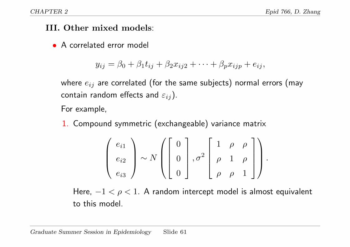
III. Other mixed models:
• A correlated error model
yij = β0 + β1tij + β2xij2 + · · ·+ βpxijp + eij ,
where eij are correlated (for the same subjects) normal errors (may
contain random effects and εij).
For example,
1. Compound symmetric (exchangeable) variance matrixei1
ei2
ei3
∼ N
0
0
0
, σ2
1 ρ ρ
ρ 1 ρ
ρ ρ 1
.
Here, −1 < ρ < 1. A random intercept model is almost equivalent
to this model.
Graduate Summer Session in Epidemiology Slide 61

CHAPTER 2 Epid 766, D. Zhang
2. AR(1) variance matrixei1
ei2
ei3
∼ N
0
0
0
, σ2
1 ρ ρ2
ρ 1 ρ
ρ2 ρ 1
.
Here, −1 < ρ < 1. It assumes that the error (ei1, ei2, ei3)T is an
autoregressive process with order 1. This structure is more
appropriate if y is measured at equally spaced time points.
3. Spatial power variance matrixei1
ei2
ei3
∼ N
0
0
0
, σ2
1 ρ|t2−t1| ρ|t3−t1|
ρ|t2−t1| 1 ρ|t3−t2|
ρ|t3−t1| ρ|t3−t2| 1
.
Here, 0 < ρ < 1. This error structure reduces to AR(1) when y is
measured at equally spaced time points. This structure is
appropriate if y is measured at unequally spaced time points.
Graduate Summer Session in Epidemiology Slide 62
CHAPTER 2 Epid 766, D. Zhang
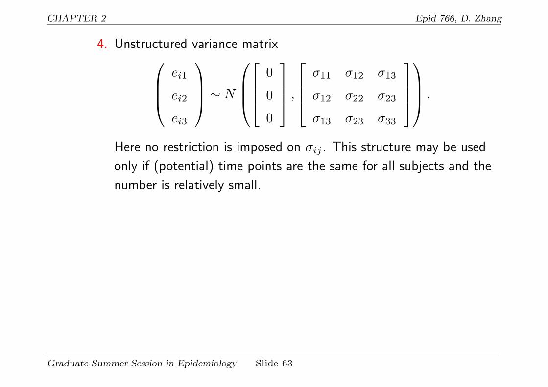
4. Unstructured variance matrixei1
ei2
ei3
∼ N
0
0
0
,σ11 σ12 σ13
σ12 σ22 σ23
σ13 σ23 σ33
.
Here no restriction is imposed on σij . This structure may be used
only if (potential) time points are the same for all subjects and the
number is relatively small.
Graduate Summer Session in Epidemiology Slide 63

CHAPTER 2 Epid 766, D. Zhang
IV. General linear mixed models
General model 1: fixed effects + random effects + pure measurement
error:
For example,
yij = β0 + β1tij + β2xij + bi0 + bi1tij + εij ,
where εij is the pure measurement error (has an independent error
structure with a constant variance).
Software to implement the above model: Proc Mixed in SAS:
Proc Mixed data= method=;class id;model y = t x / s; /* specify t x for fixed effects */random intercept t / subject=id type=un; /* specify the covariance matrix */
/* for random effects */repeated / subject=id type=vc; /* specify the variance structure for error */
run;
vc = variance component (idependent error)
Graduate Summer Session in Epidemiology Slide 64

CHAPTER 2 Epid 766, D. Zhang
General model 2: fixed effects + random effects + stochastic process
For example,
yij = β0 + β1tij + β2xij + bi0 + bi1tij + Ui(tij),
where Ui(t) is a stochastic process with AR(1), a spatial power variance
structure, or other variance structure.
Software to implement the above model: Proc Mixed in SAS:
Proc Mixed data= method=;class id;model y = t x / s; /* specify t x for fixed effects */random intercept t / subject=id type=un; /* specify the covariance matrix */
/* for random effects */repeated / subject=id type=sp(pow)(t); /* specify the variance structure for error */
run;
If the time points are equally spaced, we can use type=ar(1) in therepeated statement for AR(1) variance structure for Ui(t):
repeated cat_t / subject=id type=ar(1); /* cat_t is class t */
Graduate Summer Session in Epidemiology Slide 65
CHAPTER 2 Epid 766, D. Zhang
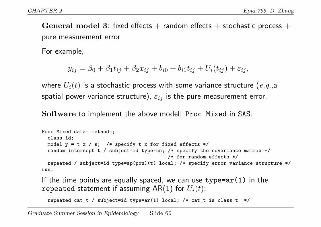
General model 3: fixed effects + random effects + stochastic process +
pure measurement error
For example,
yij = β0 + β1tij + β2xij + bi0 + bi1tij + Ui(tij) + εij ,
where Ui(t) is a stochastic process with some variance structure (e.g.,a
spatial power variance structure), εij is the pure measurement error.
Software to implement the above model: Proc Mixed in SAS:
Proc Mixed data= method=;class id;model y = t x / s; /* specify t x for fixed effects */random intercept t / subject=id type=un; /* specify the covariance matrix */
/* for random effects */repeated / subject=id type=sp(pow)(t) local; /* specify error variance structure */
run;
If the time points are equally spaced, we can use type=ar(1) in therepeated statement if assuming AR(1) for Ui(t):
repeated cat_t / subject=id type=ar(1) local; /* cat_t is class t */
Graduate Summer Session in Epidemiology Slide 66

CHAPTER 2 Epid 766, D. Zhang
General model 4: fixed effects + un-structured error
For example,
yij = β0 + β1tij + β2xij + eij ,
where eij is the error with un-structured variance matrix
Software to implement the above model: Proc Mixed in SAS:
Proc Mixed data= method=;class id;model y = t x / s; /* specify t x for fixed effects */repeated cat_t / subject=id type=un; /* specify error variance structure */
run;
Note that no “random” statement can be used in the above model. When
the number of different time points is big, there will be too many
parameters to estimate.
Graduate Summer Session in Epidemiology Slide 67

CHAPTER 2 Epid 766, D. Zhang
2.2 Estimation and inference for linear mixed
models
Let θ consist of all parms in random effects (e.g., bi0, bi1) and errors (εij).
We want to make inference on β and θ. There are two approaches:
1. Maximum likelihood:
`(β, θ; y) = logL(β, θ; y).
Maximize `(β, θ; y) jointly w.r.t. β and θ to get their MLEs.
2. Restricted maximum likelihood (REML):
(a) Get REML estimate of θ from a REML likelihood `REML(θ; y)
(take into account the estimation of β). Leads to less biased
θREML. For example, in a linear regression model
σ2REML =
Residual Sum of Squares
n− p− 1.
(b) Estimate β by maximizing `(β, θREML; y).Graduate Summer Session in Epidemiology Slide 68

CHAPTER 2 Epid 766, D. Zhang
Hypothesis Testing
• After we fit a linear mixed model such as
yij = β0 + β1tij + β2xij2 + · · ·+ βpxijp + bi0 + bi1tij + εij ,
SAS will output a test for each βk, including the estimate, SE, p-value
(for testing H0 : βk = 0), etc.
• If we want to test a contrast between βk, we can use estimate
statement in Proc Mixed. Then SAS will output the estimate, SE for
the contrast and the p-value for testing the contrast is zero. See
Programs 2 and 3 for Framingham data.
Graduate Summer Session in Epidemiology Slide 69
CHAPTER 2 Epid 766, D. Zhang
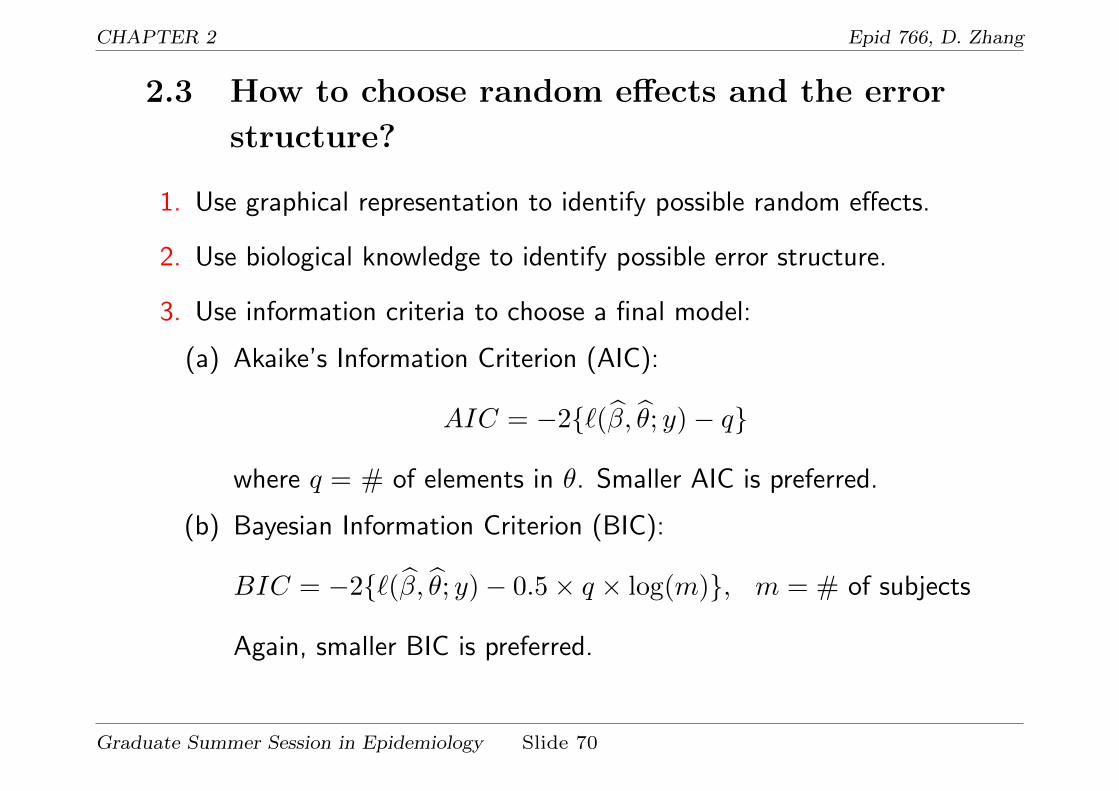
2.3 How to choose random effects and the error
structure?
1. Use graphical representation to identify possible random effects.
2. Use biological knowledge to identify possible error structure.
3. Use information criteria to choose a final model:
(a) Akaike’s Information Criterion (AIC):
AIC = −2{`(β, θ; y)− q}
where q = # of elements in θ. Smaller AIC is preferred.
(b) Bayesian Information Criterion (BIC):
BIC = −2{`(β, θ; y)− 0.5× q × log(m)}, m = # of subjects
Again, smaller BIC is preferred.
Graduate Summer Session in Epidemiology Slide 70

CHAPTER 2 Epid 766, D. Zhang
2.4 Analyze Framingham data using linear mixed
models
• Model to address objective 1: How does cholesterol level change
over time on average as people get older?
? Consider the following basic model suggested by the data:
yij = b∗i0 + b∗i1tij + εij (2.1)
where yij is the jth cholesterol level measurement from subject i,
tij is year from the beginning of the study (or baseline) and b∗i0, b∗i1
are random variables distributed as b∗i0
b∗i1
∼ N β0
β1
, σ00 σ01
σ01 σ11
,
and εij are independent errors distributed as N(0, σ2ε).
Graduate Summer Session in Epidemiology Slide 71

CHAPTER 2 Epid 766, D. Zhang
? Model (2.1) assumes that
1. The true cholesterol level for each individual changes linearly
over time with a different intercept and slope, which are both
random (since the individual is a random subject drawn from the
population).
2. Since t = 0 is the baseline, so b∗i0 can be viewed as the true but
unobserved cholesterol level for subject i at the baseline, and b∗i1can be viewed as the change rate of the true cholesterol level for
subject i.
3. β0 is the population average of the true baseline cholesterol
level of all individuals in the population, β1 is the population
average change rate of true cholesterol level and it tells us how
cholesterol level changes on average as people get older. So β1 is
the longitudinal effect or aging effect on cholesterol level.
4. σ00 is the variance of the true baseline cholesterol level b∗i0; σ11is the variance of the change rate b∗i1 of the true cholesterol level;
and σ01 is the covariance between true baseline cholesterol level
Graduate Summer Session in Epidemiology Slide 72

CHAPTER 2 Epid 766, D. Zhang
b∗i0 and the change rate b∗i1 of true cholesterol level.
? The random variables b∗i0 and b∗i1 can be re-written as
b∗i0 = β0 + bi0, b∗i1 = β1 + bi1,
where bi0, bi1 have the following distribution: bi0
bi1
∼ N 0
0
, σ00 σ01
σ01 σ11
.
? Model (2.1) then can be re-expressed as
yij = β0 + β1tij + bi0 + bi1tij + εij . (2.2)
Therefore, β0, β1 are fixed effects and bi0, bi1 are random effects.
Graduate Summer Session in Epidemiology Slide 73

CHAPTER 2 Epid 766, D. Zhang
? The following is the SAS program for fitting model (2.1):
title "Framingham data: mixed model without covariates";proc mixed data=cholst;
class newid;model cholst = time / s;random intercept time / type=un subject=newid g;repeated / type=vc subject=newid;
run;
The following is the output from the above program:
Framingham data: mixed model without covariates 1
The Mixed Procedure
Model Information
Data Set WORK.CHOLSTDependent Variable cholstCovariance Structures Unstructured, Variance
ComponentsSubject Effects newid, newidEstimation Method REMLResidual Variance Method ParameterFixed Effects SE Method Model-BasedDegrees of Freedom Method Containment
Graduate Summer Session in Epidemiology Slide 74

CHAPTER 2 Epid 766, D. Zhang
Class Level Information
Class Levels Values
newid 200 1 2 3 4 5 6 7 8 9 10 11 12 1314 ...
Dimensions
Covariance Parameters 4Columns in X 2Columns in Z Per Subject 2Subjects 200Max Obs Per Subject 6Observations Used 1044Observations Not Used 0Total Observations 1044
Iteration History
Iteration Evaluations -2 Res Log Like Criterion
0 1 10899.754336051 2 9960.12567386 0.000001202 1 9960.12082968 0.00000000
Convergence criteria met.
Graduate Summer Session in Epidemiology Slide 75

CHAPTER 2 Epid 766, D. Zhang
The Mixed Procedure
Estimated G Matrix
Row Effect newid Col1 Col2
1 Intercept 1 1467.30 -2.22592 time 1 -2.2259 3.8409
Covariance Parameter Estimates
Cov Parm Subject Estimate
UN(1,1) newid 1467.30UN(2,1) newid -2.2259UN(2,2) newid 3.8409Residual newid 434.11
Fit Statistics
-2 Res Log Likelihood 9960.1AIC (smaller is better) 9968.1AICC (smaller is better) 9968.2BIC (smaller is better) 9981.3
Null Model Likelihood Ratio Test
DF Chi-Square Pr > ChiSq
3 939.63 <.0001
Graduate Summer Session in Epidemiology Slide 76

CHAPTER 2 Epid 766, D. Zhang
Solution for Fixed Effects
StandardEffect Estimate Error DF t Value Pr > |t|
Intercept 220.57 2.9305 199 75.26 <.0001time 2.8170 0.2408 191 11.70 <.0001
Type 3 Tests of Fixed Effects
Num DenEffect DF DF F Value Pr > F
time 1 191 136.83 <.0001
From this output, we see that:
1. σ00 = 1467, as compared to var(b0) = 1738 from the two-stage
approach.
2. σ11 = 3.84, as compared to var(b1) = 13.2 from the two-stage
approach.
3. corr(b∗i0, b∗i1) = corr(bi0, bi1) = −2.2259/
√1467× 3.84 = −0.03,
as compared to corr(b0, b1) = −0.27 from the two-stage approach.
4. The estimated mean of true baseline cholesterol level is
β0 = 220.57 with SE=2.93, as compared to the sample mean
Graduate Summer Session in Epidemiology Slide 77
CHAPTER 2 Epid 766, D. Zhang
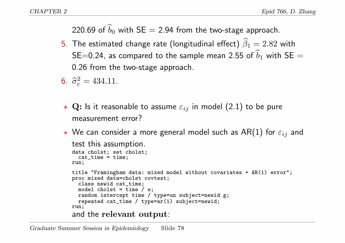
220.69 of b0 with SE = 2.94 from the two-stage approach.
5. The estimated change rate (longitudinal effect) β1 = 2.82 with
SE=0.24, as compared to the sample mean 2.55 of b1 with SE =
0.26 from the two-stage approach.
6. σ2ε = 434.11.
? Q: Is it reasonable to assume εij in model (2.1) to be pure
measurement error?
? We can consider a more general model such as AR(1) for εij and
test this assumption.data cholst; set cholst;
cat_time = time;run;
title "Framingham data: mixed model without covariates + AR(1) error";proc mixed data=cholst covtest;
class newid cat_time;model cholst = time / s;random intercept time / type=un subject=newid g;repeated cat_time / type=ar(1) subject=newid;
run;
and the relevant output:
Graduate Summer Session in Epidemiology Slide 78
CHAPTER 2 Epid 766, D. Zhang
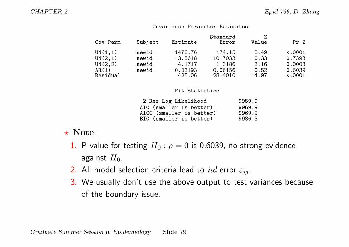
Covariance Parameter Estimates
Standard ZCov Parm Subject Estimate Error Value Pr Z
UN(1,1) newid 1478.76 174.15 8.49 <.0001UN(2,1) newid -3.5618 10.7033 -0.33 0.7393UN(2,2) newid 4.1717 1.3186 3.16 0.0008AR(1) newid -0.03193 0.06156 -0.52 0.6039Residual 425.06 28.4010 14.97 <.0001
Fit Statistics
-2 Res Log Likelihood 9959.9AIC (smaller is better) 9969.9AICC (smaller is better) 9969.9BIC (smaller is better) 9986.3
? Note:
1. P-value for testing H0 : ρ = 0 is 0.6039, no strong evidence
against H0.
2. All model selection criteria lead to iid error εij .
3. We usually don’t use the above output to test variances because
of the boundary issue.
Graduate Summer Session in Epidemiology Slide 79
CHAPTER 2 Epid 766, D. Zhang
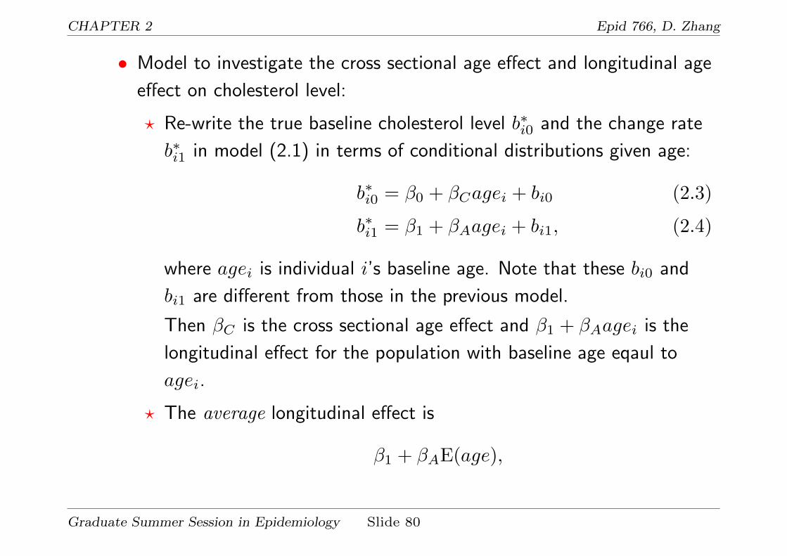
• Model to investigate the cross sectional age effect and longitudinal age
effect on cholesterol level:
? Re-write the true baseline cholesterol level b∗i0 and the change rate
b∗i1 in model (2.1) in terms of conditional distributions given age:
b∗i0 = β0 + βCagei + bi0 (2.3)
b∗i1 = β1 + βAagei + bi1, (2.4)
where agei is individual i’s baseline age. Note that these bi0 and
bi1 are different from those in the previous model.
Then βC is the cross sectional age effect and β1 + βAagei is the
longitudinal effect for the population with baseline age eqaul to
agei.
? The average longitudinal effect is
β1 + βAE(age),
Graduate Summer Session in Epidemiology Slide 80

CHAPTER 2 Epid 766, D. Zhang
which can be estimated by
β1 + βAage,
where age is the sample average of age.
? Suggest that we can center age and use the centered age (denoted
by cent agei = agei − age) in (2.3). Then β1 is the average
longitudinal effect
? We are interested in testing H0 : βC = β1.
? Assume the usual distribution for (bi0, bi1): bi0
bi1
∼ N 0
0
, σ00 σ01
σ01 σ11
.
Here both σ00 and σ11 are the remaining variances in b∗i0 and b∗i1after baseline age effect has been taken into account. So they
should be smaller than those corresponding values in model (2.1).
Graduate Summer Session in Epidemiology Slide 81
CHAPTER 2 Epid 766, D. Zhang
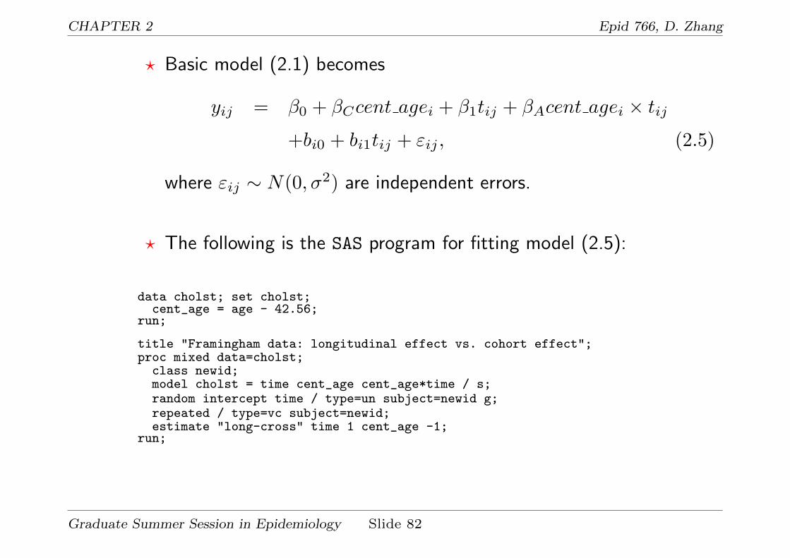
? Basic model (2.1) becomes
yij = β0 + βCcent agei + β1tij + βAcent agei × tij+bi0 + bi1tij + εij , (2.5)
where εij ∼ N(0, σ2) are independent errors.
? The following is the SAS program for fitting model (2.5):
data cholst; set cholst;cent_age = age - 42.56;
run;
title "Framingham data: longitudinal effect vs. cohort effect";proc mixed data=cholst;
class newid;model cholst = time cent_age cent_age*time / s;random intercept time / type=un subject=newid g;repeated / type=vc subject=newid;estimate "long-cross" time 1 cent_age -1;
run;
Graduate Summer Session in Epidemiology Slide 82

CHAPTER 2 Epid 766, D. Zhang
? The relevant output of the above SAS program is
Iteration History
Iteration Evaluations -2 Res Log Like Criterion
0 1 10826.015763001 2 9929.74817925 0.000005162 1 9929.72729664 0.00000000
Convergence criteria met.
Estimated G Matrix
Row Effect newid Col1 Col2
1 Intercept 1 1226.69 9.78292 time 1 9.7829 3.2598
Covariance Parameter Estimates
Cov Parm Subject Estimate
UN(1,1) newid 1226.69UN(2,1) newid 9.7829UN(2,2) newid 3.2598Residual newid 434.15
Fit Statistics
-2 Res Log Likelihood 9929.7AIC (smaller is better) 9937.7
Graduate Summer Session in Epidemiology Slide 83
CHAPTER 2 Epid 766, D. Zhang
AICC (smaller is better) 9937.8BIC (smaller is better) 9950.9
Null Model Likelihood Ratio Test
DF Chi-Square Pr > ChiSq
3 896.29 <.0001
Solution for Fixed Effects
StandardEffect Estimate Error DF t Value Pr > |t|
Intercept 220.57 2.7172 198 81.18 <.0001time 2.8157 0.2343 190 12.02 <.0001cent_age 1.9861 0.3455 652 5.75 <.0001time*cent_age -0.1024 0.02930 652 -3.50 0.0005
Type 3 Tests of Fixed Effects
Num DenEffect DF DF F Value Pr > F
time 1 190 144.42 <.0001cent_age 1 652 33.05 <.0001time*cent_age 1 652 12.22 0.0005
Estimates
StandardLabel Estimate Error DF t Value Pr > |t|
long-cross 0.8296 0.4174 652 1.99 0.0473
Graduate Summer Session in Epidemiology Slide 84
CHAPTER 2 Epid 766, D. Zhang
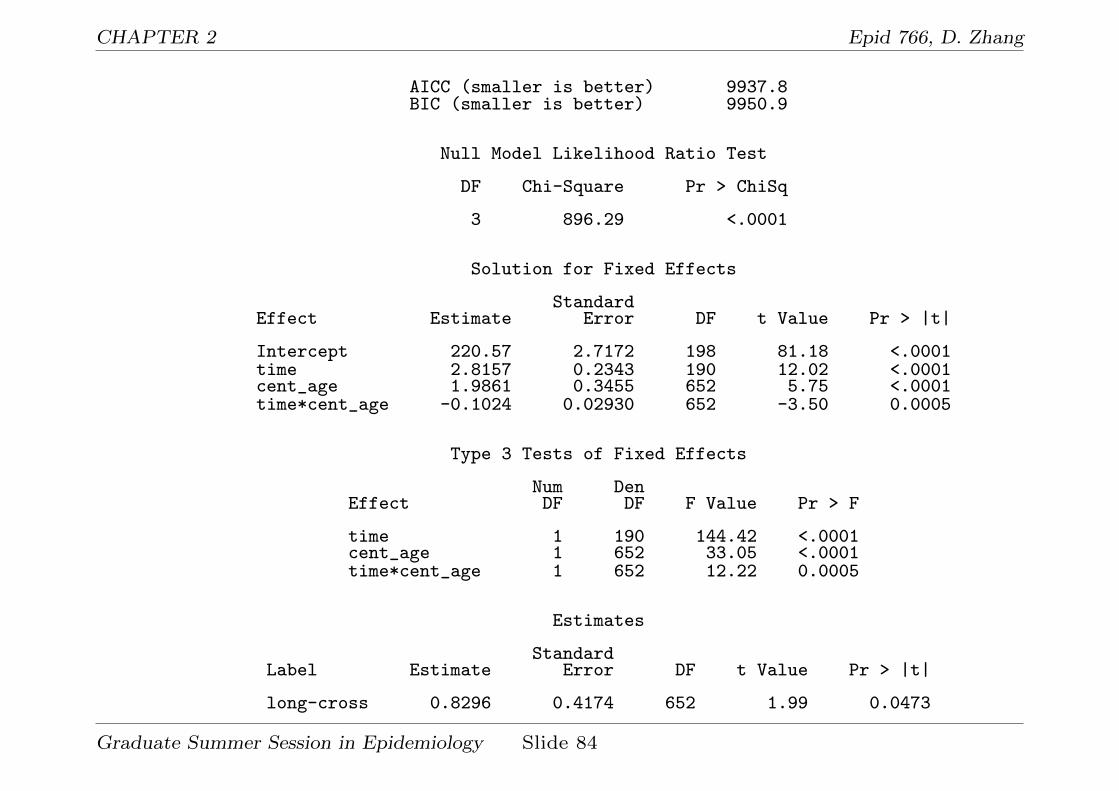
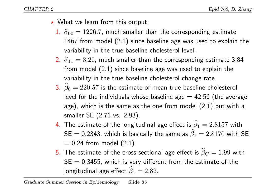
? What we learn from this output:
1. σ00 = 1226.7, much smaller than the corresponding estimate
1467 from model (2.1) since baseline age was used to explain the
variability in the true baseline cholesterol level.
2. σ11 = 3.26, much smaller than the corresponding estimate 3.84
from model (2.1) since baseline age was used to explain the
variability in the true baseline cholesterol change rate.
3. β0 = 220.57 is the estimate of mean true baseline cholesterol
level for the individuals whose baseline age = 42.56 (the average
age), which is the same as the one from model (2.1) but with a
smaller SE (2.71 vs. 2.93).
4. The estimate of the longitudinal age effect is β1 = 2.8157 with
SE = 0.2343, which is basically the same as β1 = 2.8170 with SE
= 0.24 from model (2.1).
5. The estimate of the cross sectional age effect is βC = 1.99 with
SE = 0.3455, which is very different from the estimate of the
longitudinal age effect β1 = 2.82.
Graduate Summer Session in Epidemiology Slide 85

CHAPTER 2 Epid 766, D. Zhang
6. The P-value for testing H0 : βL = βC is 0.0473, significant at
level 0.05!
7. σ2ε = 434.15 is basically the same as the corresponding estimate
from model (2.1), which is 434.11.
8. Similarly, we can test iid εij by considering correlated errors such
as AR(1) for εij and test to see if ρ = 0.
Graduate Summer Session in Epidemiology Slide 86
CHAPTER 2 Epid 766, D. Zhang
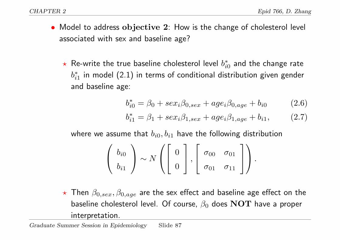
• Model to address objective 2: How is the change of cholesterol level
associated with sex and baseline age?
? Re-write the true baseline cholesterol level b∗i0 and the change rate
b∗i1 in model (2.1) in terms of conditional distribution given gender
and baseline age:
b∗i0 = β0 + sexiβ0,sex + ageiβ0,age + bi0 (2.6)
b∗i1 = β1 + sexiβ1,sex + ageiβ1,age + bi1, (2.7)
where we assume that bi0, bi1 have the following distribution bi0
bi1
∼ N 0
0
, σ00 σ01
σ01 σ11
.
? Then β0,sex, β0,age are the sex effect and baseline age effect on the
baseline cholesterol level. Of course, β0 does NOT have a proper
interpretation.Graduate Summer Session in Epidemiology Slide 87

CHAPTER 2 Epid 766, D. Zhang
? Similarly, β1,sex, β1,age are the sex effect and baseline age effect on
the change rate of the true cholesterol level, and β1 does NOT
have a proper interpretation.
? Substituting the above expressions into model (2.1), we got
yij = β0 + sexiβ0,sex + ageiβ0,age + β1tij
+sexitijβ1,sex + ageitijβ1,age + bi0 + bi1tij + εij . (2.8)
? Suppose we also want to test whether or not the change rates
between 30 years old males and 40 years old females are the same
using the above model.
? From model (2.7), the (average) change rate of 30 years old males
is
β1 + 1× β1,sex + 30× β1,age = β1 + β1,sex + 30β1,age.
Graduate Summer Session in Epidemiology Slide 88
CHAPTER 2 Epid 766, D. Zhang
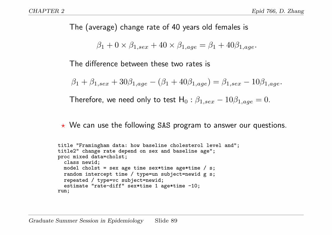
The (average) change rate of 40 years old females is
β1 + 0× β1,sex + 40× β1,age = β1 + 40β1,age.
The difference between these two rates is
β1 + β1,sex + 30β1,age − (β1 + 40β1,age) = β1,sex − 10β1,age.
Therefore, we need only to test H0 : β1,sex − 10β1,age = 0.
? We can use the following SAS program to answer our questions.
title "Framingham data: how baseline cholesterol level and";title2" change rate depend on sex and baseline age";proc mixed data=cholst;
class newid;model cholst = sex age time sex*time age*time / s;random intercept time / type=un subject=newid g s;repeated / type=vc subject=newid;estimate "rate-diff" sex*time 1 age*time -10;
run;
Graduate Summer Session in Epidemiology Slide 89

CHAPTER 2 Epid 766, D. Zhang
? Part of the relevant output from above program is
Framingham data: how baseline cholesterol level and 1change rate depend on sex and baseline age
Iteration History
Iteration Evaluations -2 Res Log Like Criterion
0 1 10813.995871541 2 9907.89014721 0.000006552 1 9907.86364103 0.00000000
Convergence criteria met.
Estimated G Matrix
Row Effect newid Col1 Col2
1 Intercept 1 1209.89 13.55022 time 1 13.5502 2.5211
Covariance Parameter Estimates
Cov Parm Subject Estimate
UN(1,1) newid 1209.89UN(2,1) newid 13.5502UN(2,2) newid 2.5211Residual newid 434.15
Graduate Summer Session in Epidemiology Slide 90
CHAPTER 2 Epid 766, D. Zhang
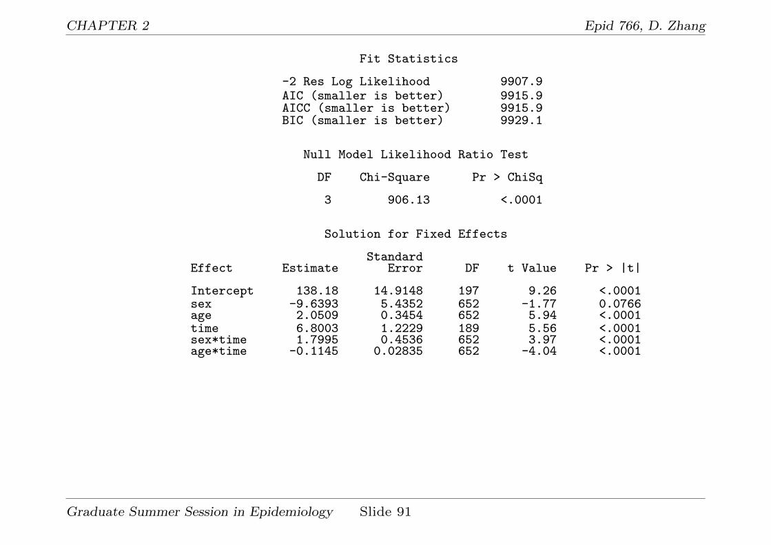
Fit Statistics
-2 Res Log Likelihood 9907.9AIC (smaller is better) 9915.9AICC (smaller is better) 9915.9BIC (smaller is better) 9929.1
Null Model Likelihood Ratio Test
DF Chi-Square Pr > ChiSq
3 906.13 <.0001
Solution for Fixed Effects
StandardEffect Estimate Error DF t Value Pr > |t|
Intercept 138.18 14.9148 197 9.26 <.0001sex -9.6393 5.4352 652 -1.77 0.0766age 2.0509 0.3454 652 5.94 <.0001time 6.8003 1.2229 189 5.56 <.0001sex*time 1.7995 0.4536 652 3.97 <.0001age*time -0.1145 0.02835 652 -4.04 <.0001
Graduate Summer Session in Epidemiology Slide 91

CHAPTER 2 Epid 766, D. Zhang
Solution for Random Effects
Std ErrEffect newid Estimate Pred DF t Value Pr > |t|
Intercept 2 100.50 11.5761 651 8.68 <.0001time 2 2.7414 1.2643 651 2.17 0.0305Intercept 74 46.9844 11.0096 651 4.27 <.0001time 74 1.3579 1.2525 651 1.08 0.2787Intercept 171 -51.5764 11.3046 651 -4.56 <.0001time 171 -0.6812 1.2583 651 -0.54 0.5885
Estimates
StandardLabel Estimate Error DF t Value Pr > |t|
rate-diff 2.9441 0.5606 651 5.25 <.0001
Graduate Summer Session in Epidemiology Slide 92

CHAPTER 2 Epid 766, D. Zhang
? What we learn from this output:
1. β0,sex = −9.64 (SE = 5.43), so after adjusting for baseline age,
males’ baseline cholesterol level is about 10 units less than
females’.
2. β0,age = 2.05 (SE = 0.35), so after adjusting for gender, one
year older people’s baseline cholesterol level is about 2 units
higher than that of one year younger people.
3. β1,sex = 1.80 (SE = 0.45), so after adjusting for baseline age,
males’ change rate is 1.80 (cholesterol unit/year) greater that
females’ change rate. Similar estimate from 2-stage analysis is
1.74 (SE=0.49).
4. β1,age = −0.11 (SE = 0.028), so after adjusting for sex, one year
older people’s change rate is 0.11 less than one year younger
people’s change rate. Similar estimate from 2-stage analysis is
-0.11 (SE=0.031).
5. The change rate difference of interest is 2.94 (SE = 0.56).
Significantly different!
Graduate Summer Session in Epidemiology Slide 93

CHAPTER 2 Epid 766, D. Zhang
6. σ00 = 1210, which is smaller than the corresponding estimate
from model (2.5) since we use both age and gender to explain
the variability in baseline true cholesterol level.
7. σ11 = 2.52, which is smaller than the corresponding estimate
from model (2.5) since we use both age and gender to explain
the variability in the cholesterol level change rate.
8. σ2ε = 434.15, basically the same as its estimates from models
(2.1) and (2.5).
9. Similarly, we can test iid εij by considering correlated errors such
as AR(1).
? Note: The models (2.6) and (2.7) for b∗i0 and b∗i1 are basically the
same as the second stage models in the two stage analysis for the
Framingham data.
? Compare results from this model to the results from the two-stage
analysis:
Graduate Summer Session in Epidemiology Slide 94

CHAPTER 2 Epid 766, D. Zhang
(a) Effect on baseline cholesterol level:
Model (2.8) : β0 = 138.18(SE = 14.9),
β0,sex = −9.64(SE = 5.43), β0,age = 2.05(SE = 0.35)
Two-stage : α0 = 138.2(SE = 15.0),
α1 = −9.75(SE = 5.48), α2 = 2.06(SE = 0.35).
(b) Effect on change rate of cholesterol level:
Model (2.8) : β1 = 6.80(SE = 1.22),
β1,sex = 1.80(SE = 0.45), β1,age = −0.11(SE = 0.03).
Two-stage : β0 = 6.14(SE = 1.35),
β1 = 1.74(SE = 0.49), β2 = −0.11(SE = 0.03).
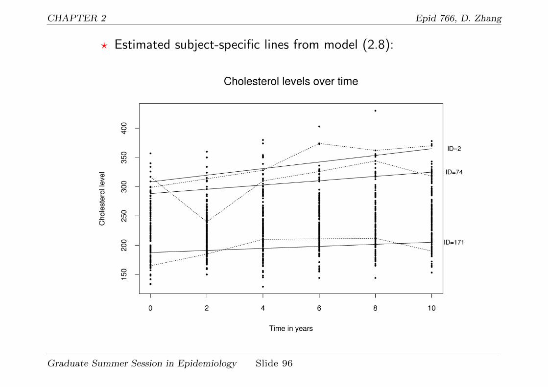
? We can also estimate the individual random effects and estimate
their trajectory lines.
Graduate Summer Session in Epidemiology Slide 95
CHAPTER 2 Epid 766, D. Zhang
? Estimated subject-specific lines from model (2.8):
Graduate Summer Session in Epidemiology Slide 96

CHAPTER 2 Epid 766, D. Zhang
• Model to address Objective 3: Do males have more stable (true)
baseline cholesterol level and change rate than females?
? From model (2.1), assume b∗i0, b∗i1 have different distributions for
males and females:
Males:
b∗i0
b∗i1
∼ N µm0
µm1
, σm00 σm01
σm01 σm11
Females:
b∗i0
b∗i1
∼ N µf0
µf1
, σf00 σf01
σf01 σf11
(2.9)
? We would like to test H0 : σm00 = σf00, σm01 = σf01, σm11 = σf11
(i.e., the above two variance-covariance matrices are the same).
Graduate Summer Session in Epidemiology Slide 97

CHAPTER 2 Epid 766, D. Zhang
? The SAS program and its output for fitting above model are as
follows:data cholst; set cholst;
gender=sex;run;
title "Framingham data: do males have more stable (true) baseline";title2 "cholesterol level and change rate than females?";proc mixed data=cholst;
class newid gender;model cholst = sex time sex*time / s;random intercept time / type=un subject=newid group=gender g;repeated / type=vc subject=newid;
run;
Framingham data: do males have more stable (true) baseline 1cholesterol level and change rate than females?
The Mixed Procedure
Iteration History
Iteration Evaluations -2 Res Log Like Criterion
0 1 10889.094795291 3 9939.57691271 0.000003172 1 9939.56399905 0.00000000
The Mixed Procedure
Convergence criteria met.
Graduate Summer Session in Epidemiology Slide 98

CHAPTER 2 Epid 766, D. Zhang
Estimated G Matrix
Row Effect newid gender Col1 Col2 Col3 Col4
1 Intercept 1 0 1402.47 -4.70152 time 1 0 -4.7015 1.82793 Intercept 1 1 1532.81 3.61194 time 1 1 3.6119 4.7970
Covariance Parameter Estimates
Cov Parm Subject Group Estimate
UN(1,1) newid gender 0 1402.47UN(2,1) newid gender 0 -4.7015UN(2,2) newid gender 0 1.8279UN(1,1) newid gender 1 1532.81UN(2,1) newid gender 1 3.6119UN(2,2) newid gender 1 4.7970Residual newid 433.71
Fit Statistics
-2 Res Log Likelihood 9939.6AIC (smaller is better) 9953.6AICC (smaller is better) 9953.7BIC (smaller is better) 9976.7
Graduate Summer Session in Epidemiology Slide 99
CHAPTER 2 Epid 766, D. Zhang
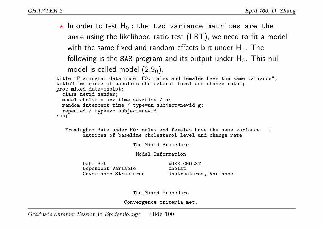
? In order to test H0 : the two variance matrices are the
same using the likelihood ratio test (LRT), we need to fit a model
with the same fixed and random effects but under H0. The
following is the SAS program and its output under H0. This null
model is called model (2.90).title "Framingham data under H0: males and females have the same variance";title2 "matrices of baseline cholesterol level and change rate";proc mixed data=cholst;
class newid gender;model cholst = sex time sex*time / s;random intercept time / type=un subject=newid g;repeated / type=vc subject=newid;
run;
Framingham data under H0: males and females have the same variance 1matrices of baseline cholesterol level and change rate
The Mixed Procedure
Model Information
Data Set WORK.CHOLSTDependent Variable cholstCovariance Structures Unstructured, Variance
The Mixed Procedure
Convergence criteria met.
Graduate Summer Session in Epidemiology Slide 100

CHAPTER 2 Epid 766, D. Zhang
Estimated G Matrix
Row Effect newid Col1 Col2
1 Intercept 1 1465.85 -0.25162 time 1 -0.2516 3.2618
Covariance Parameter Estimates
Cov Parm Subject Estimate
UN(1,1) newid 1465.85UN(2,1) newid -0.2516UN(2,2) newid 3.2618Residual newid 434.17
Fit Statistics
-2 Res Log Likelihood 9943.0AIC (smaller is better) 9951.0AICC (smaller is better) 9951.1BIC (smaller is better) 9964.2
? The difference of -2 residual log likelihood is 9943 - 9939.6
= 3.4 (between models (2.9) and (2.90)) and the P-value =
P [χ23 ≥ 3.4] = 0.33.
Graduate Summer Session in Epidemiology Slide 101
CHAPTER 2 Epid 766, D. Zhang
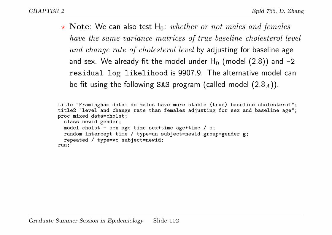
? Note: We can also test H0: whether or not males and females
have the same variance matrices of true baseline cholesterol level
and change rate of cholesterol level by adjusting for baseline age
and sex. We already fit the model under H0 (model (2.8)) and -2
residual log likelihood is 9907.9. The alternative model can
be fit using the following SAS program (called model (2.8A)).
title "Framingham data: do males have more stable (true) baseline cholesterol";title2 "level and change rate than females adjusting for sex and baseline age";proc mixed data=cholst;
class newid gender;model cholst = sex age time sex*time age*time / s;random intercept time / type=un subject=newid group=gender g;repeated / type=vc subject=newid;
run;
Graduate Summer Session in Epidemiology Slide 102
CHAPTER 2 Epid 766, D. Zhang
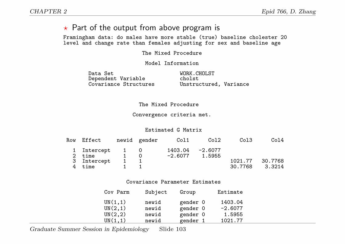
? Part of the output from above program isFramingham data: do males have more stable (true) baseline cholester 20level and change rate than females adjusting for sex and baseline age
The Mixed Procedure
Model Information
Data Set WORK.CHOLSTDependent Variable cholstCovariance Structures Unstructured, Variance
The Mixed Procedure
Convergence criteria met.
Estimated G Matrix
Row Effect newid gender Col1 Col2 Col3 Col4
1 Intercept 1 0 1403.04 -2.60772 time 1 0 -2.6077 1.59553 Intercept 1 1 1021.77 30.77684 time 1 1 30.7768 3.3214
Covariance Parameter Estimates
Cov Parm Subject Group Estimate
UN(1,1) newid gender 0 1403.04UN(2,1) newid gender 0 -2.6077UN(2,2) newid gender 0 1.5955UN(1,1) newid gender 1 1021.77
Graduate Summer Session in Epidemiology Slide 103

CHAPTER 2 Epid 766, D. Zhang
UN(2,1) newid gender 1 30.7768UN(2,2) newid gender 1 3.3214Residual newid 434.93
Fit Statistics
-2 Res Log Likelihood 9901.6AIC (smaller is better) 9915.6AICC (smaller is better) 9915.7BIC (smaller is better) 9938.7
? The -2 residual log likelihood is 9901.6 so difference is
9907.9-9901.6 = 6.3. The P-value = P [χ23 ≥ 6.3] = 0.09, more
evidence against H0.
Graduate Summer Session in Epidemiology Slide 104

CHAPTER 2 Epid 766, D. Zhang
Comparison of fit statistics among models
Model AIC BIC
Model (2.1) 9968.1 9981.3
Model (2.5) 9937. 9950.9
Model (2.8) 9915.9 9929.1
Model (2.9) 9953.6 9976.7
Model (2.90) 9951.0 9964.2
Model (2.8A) 9915.6 9938.7
Graduate Summer Session in Epidemiology Slide 105

CHAPTER 2 Epid 766, D. Zhang
• Note:
1. The choice of model, especially the fixed effects terms, depends on
the questions we need to answer. However, we can use AIC or BIC
to determine the random effects and the error structure.
2. If we want a model with the most prediction power, we can
consider a complicated model with AIC or BIC as a guide for model
selection.
3. It seems that model (2.8) is the winner among the above models if
we are looking for a model with the most predictive power.
Graduate Summer Session in Epidemiology Slide 106
CHAPTER 2 Epid 766, D. Zhang
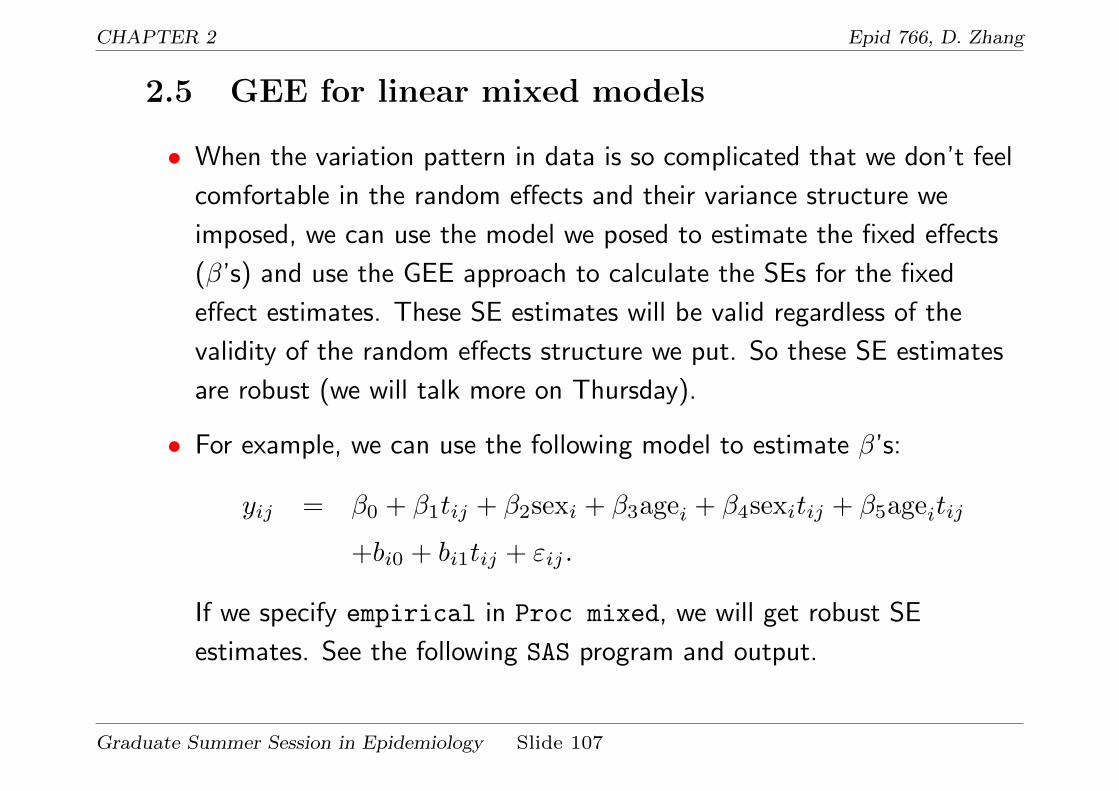
2.5 GEE for linear mixed models
• When the variation pattern in data is so complicated that we don’t feel
comfortable in the random effects and their variance structure we
imposed, we can use the model we posed to estimate the fixed effects
(β’s) and use the GEE approach to calculate the SEs for the fixed
effect estimates. These SE estimates will be valid regardless of the
validity of the random effects structure we put. So these SE estimates
are robust (we will talk more on Thursday).
• For example, we can use the following model to estimate β’s:
yij = β0 + β1tij + β2sexi + β3agei + β4sexitij + β5ageitij
+bi0 + bi1tij + εij .
If we specify empirical in Proc mixed, we will get robust SE
estimates. See the following SAS program and output.
Graduate Summer Session in Epidemiology Slide 107

CHAPTER 2 Epid 766, D. Zhang
title "Using GEE to fit Framingham data";proc mixed data=cholst empirical;
class newid;model cholst = time sex age sex*time age*time / s;random intercept time / type=un subject=newid;repeated / type=vc subject=newid;
run;
Output of the above program
Using GEE to fit Framingham data 24
The Mixed Procedure
Model Information
Data Set WORK.CHOLSTDependent Variable cholstCovariance Structures Unstructured, Variance
ComponentsSubject Effects newid, newidEstimation Method REMLResidual Variance Method ParameterFixed Effects SE Method EmpiricalDegrees of Freedom Method Containment
Iteration History
Iteration Evaluations -2 Res Log Like Criterion
0 1 10813.995871541 2 9907.89014721 0.000006552 1 9907.86364103 0.00000000
Convergence criteria met.
Graduate Summer Session in Epidemiology Slide 108

CHAPTER 2 Epid 766, D. Zhang
The Mixed Procedure
Covariance Parameter Estimates
Cov Parm Subject Estimate
UN(1,1) newid 1209.89UN(2,1) newid 13.5502UN(2,2) newid 2.5211Residual newid 434.15
Fit Statistics
-2 Res Log Likelihood 9907.9AIC (smaller is better) 9915.9AICC (smaller is better) 9915.9BIC (smaller is better) 9929.1
Null Model Likelihood Ratio Test
DF Chi-Square Pr > ChiSq
3 906.13 <.0001
Solution for Fixed Effects
StandardEffect Estimate Error DF t Value Pr > |t|
Intercept 138.18 15.4017 197 8.97 <.0001sex -9.6393 5.4588 651 -1.77 0.0779age 2.0509 0.3749 651 5.47 <.0001time 6.8003 1.2188 190 5.58 <.0001time*sex 1.7995 0.4524 651 3.98 <.0001time*age -0.1145 0.02868 651 -3.99 <.0001
Graduate Summer Session in Epidemiology Slide 109

CHAPTER 2 Epid 766, D. Zhang
What we observed:
1. Fixed effects estimates and variance-covariance parameter estimates
are exactly the same as those from model (2.8).
2. The SEs for the fixed effects estimates are different from those from
model (2.8). However, they are very close, indicating model (2.8) has
a reasonably good fit to the data and we don’t have to use the GEE
approach.
Graduate Summer Session in Epidemiology Slide 110
CHAPTER 2 Epid 766, D. Zhang
2.6 Missing data issues
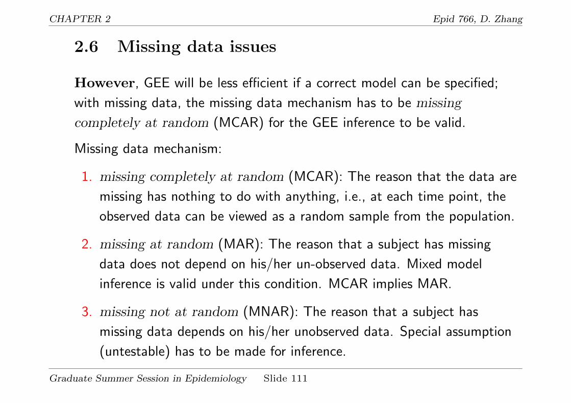
However, GEE will be less efficient if a correct model can be specified;
with missing data, the missing data mechanism has to be missing
completely at random (MCAR) for the GEE inference to be valid.
Missing data mechanism:
1. missing completely at random (MCAR): The reason that the data are
missing has nothing to do with anything, i.e., at each time point, the
observed data can be viewed as a random sample from the population.
2. missing at random (MAR): The reason that a subject has missing
data does not depend on his/her un-observed data. Mixed model
inference is valid under this condition. MCAR implies MAR.
3. missing not at random (MNAR): The reason that a subject has
missing data depends on his/her unobserved data. Special assumption
(untestable) has to be made for inference.
Graduate Summer Session in Epidemiology Slide 111

CHAPTER 2 Epid 766, D. Zhang
Ways to assess MCAR
1. Suppose the missing data pattern (for y) looks like
Time points
1 2 3
?
? ?
and assume x (such as age) is a completely observed variable.
2. Compare x for the two groups with observed y and missing y at times
2 and 3 (using, say, two-sample t-test). A significant difference
indicates the violation of MCAR. Otherwise, you may feel comfortable
about the MCAR assumption.
Remark: MAR cannot be tested.
Graduate Summer Session in Epidemiology Slide 112
CHAPTER 2 Epid 766, D. Zhang
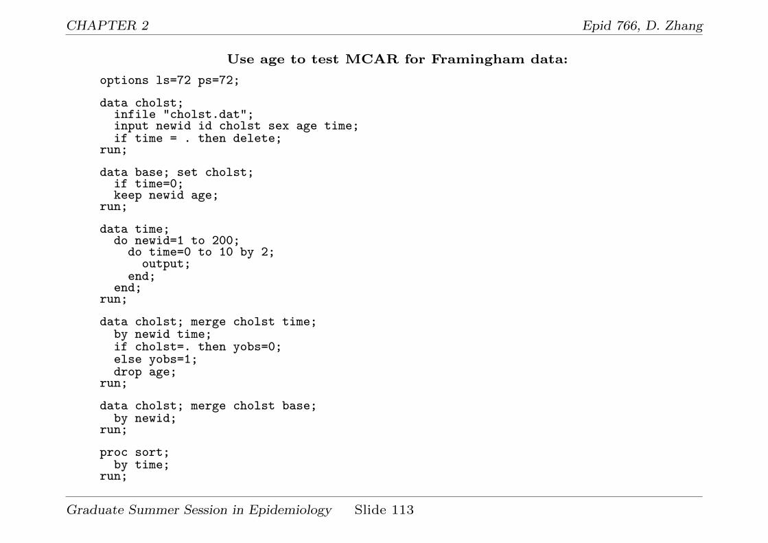
Use age to test MCAR for Framingham data:
options ls=72 ps=72;
data cholst;infile "cholst.dat";input newid id cholst sex age time;if time = . then delete;
run;
data base; set cholst;if time=0;keep newid age;
run;
data time;do newid=1 to 200;
do time=0 to 10 by 2;output;
end;end;
run;
data cholst; merge cholst time;by newid time;if cholst=. then yobs=0;else yobs=1;drop age;
run;
data cholst; merge cholst base;by newid;
run;
proc sort;by time;
run;
Graduate Summer Session in Epidemiology Slide 113

CHAPTER 2 Epid 766, D. Zhang
title "Test equality of age between missing and non-missing groups";proc ttest;
var age;class yobs;by time;
run;
SAS output:
Test equality of age between missing and non-missing groups 1
-------------------------------- time=2 --------------------------------
The TTEST Procedure
T-Tests
Variable Method Variances DF t Value Pr > |t|
age Pooled Equal 198 0.35 0.7298age Satterthwaite Unequal 29.6 0.35 0.7325
-------------------------------- time=4 --------------------------------
The TTEST Procedure
T-Tests
Variable Method Variances DF t Value Pr > |t|
age Pooled Equal 198 -0.23 0.8172age Satterthwaite Unequal 39.5 -0.22 0.8304
Graduate Summer Session in Epidemiology Slide 114

CHAPTER 2 Epid 766, D. Zhang
-------------------------------- time=6 ---------------------------------
T-Tests
Variable Method Variances DF t Value Pr > |t|
age Pooled Equal 198 1.43 0.1536age Satterthwaite Unequal 40.3 1.37 0.1774
-------------------------------- time=8 --------------------------------
T-Tests
Variable Method Variances DF t Value Pr > |t|
age Pooled Equal 198 0.47 0.6418age Satterthwaite Unequal 47 0.50 0.6179
------------------------------- time=10 --------------------------------
T-Tests
Variable Method Variances DF t Value Pr > |t|
age Pooled Equal 198 0.24 0.8071age Satterthwaite Unequal 63.3 0.27 0.7879
Graduate Summer Session in Epidemiology Slide 115
CHAPTER 3 Epid 766, D. Zhang
3 Modeling and design issues
• How to handle baseline response?
• Do we model previous responses as covariates?
• Modeling response vs. modeling the change of response
• A simulation study comparing modeling response to modeling its
change
• Design a longitudinal study. Sample size calculation
1. Comparing time-averaged means
2. Comparing slopes
Graduate Summer Session in Epidemiology Slide 116

CHAPTER 3 Epid 766, D. Zhang
3.1 How to handle baseline response?
• Model baseline outcome as part of the response. For example,
yij = β0 + β1xij + εij , i = 1, ...,m, j = 1, 2, ..., ni, (3.1)
where the errors εij include random effects and other errors, and hence
are correlated. For example, εij = bi + εij for a random intercept
model.
• Model baseline outcome as a covariate. For example,
yij = β0 + β1xij + β2yi1 + eij , i = 1, ...,m, j = 2, ..., ni. (3.2)
Comments:
1. There are some subtle difference between these two models. The
regression parameters β0, β1 and the variance components have
different interpretation and hence we will get different estimates from
two models. β1 in model (3.1) is the overall effect of x on y, while β1
Graduate Summer Session in Epidemiology Slide 117

CHAPTER 3 Epid 766, D. Zhang
in model (3.2) is the adjusted covariate effect of x on y adjusting for
baseline response.
2. Model (3.2) is more convenient for prediction. Although one can also
get a prediction model similar to model (3.2) by conditioning on the
baseline response from model (3.1).
3. When baseline response yi1 is used as a covariate, it CANNOT be
re-used in the outcome variable. For model (3.2), index j goes from 2
to ni. Because of this, the estimates from model (3.1) may be more
efficient.
4. It is obvious that in the presence of missing data, the subjects with
baseline measurements only will be deleted from the analysis if model
(3.2) is used. In the case where missingness depends on the baseline
measurements, inference using model (3.2) will be invalid. However,
model (3.1) will still give valid inference. We will see a simulation
study later.
Graduate Summer Session in Epidemiology Slide 118
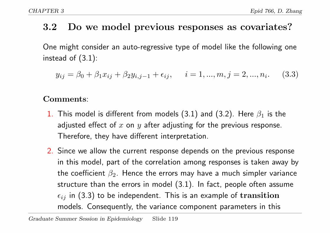
CHAPTER 3 Epid 766, D. Zhang
3.2 Do we model previous responses as covariates?
One might consider an auto-regressive type of model like the following one
instead of (3.1):
yij = β0 + β1xij + β2yi,j−1 + εij , i = 1, ...,m, j = 2, ..., ni. (3.3)
Comments:
1. This model is different from models (3.1) and (3.2). Here β1 is the
adjusted effect of x on y after adjusting for the previous response.
Therefore, they have different interpretation.
2. Since we allow the current response depends on the previous response
in this model, part of the correlation among responses is taken away by
the coefficient β2. Hence the errors may have a much simpler variance
structure than the errors in model (3.1). In fact, people often assume
εij in (3.3) to be independent. This is an example of transition
models. Consequently, the variance component parameters in this
Graduate Summer Session in Epidemiology Slide 119

CHAPTER 3 Epid 766, D. Zhang
model are different and have different interpretation from those in
model (3.1).
3. We can obtain a similar model to this one if we assume the errors in
model (3.1) have an AR(1) variance structure.
4. Similar to model (3.2), this model is more convenient for prediction.
5. Similar to model (3.2), subjects with baseline measurements only will
be deleted from the analysis. If missingness of subsequent
measurements depends on the baseline measurements, this model will
give invalid inference on the parameters of interest.
Graduate Summer Session in Epidemiology Slide 120

CHAPTER 3 Epid 766, D. Zhang
3.3 Modeling outcome vs. modeling the change of
outcome
Define change from baseline:
Dij = yij − yi1, i = 1, ...,m, j = 2, ..., ni
and consider model
Dij = β0 + β1xij + εij , i = 1, ...,m, j = 2, ..., ni. (3.4)
Comments:
1. This model emphasizes the effect of x on the change (from baseline
value) of outcome. Therefore, β1 has different interpretation than the
β1’s in previous models.
2. Since we are modeling the difference, part of the correlation in the
responses due to among individual variation is removed. Therefore, the
errors in this model will have a simpler variance structure than model
Graduate Summer Session in Epidemiology Slide 121

CHAPTER 3 Epid 766, D. Zhang
(3.1), and the parameters in the variance structures have different
interpretation.
3. Baseline outcome yi1 can be used as a covariate.
4. It cannot model how x affects the overall mean of outcome.
5. Similar to models (3.2) and (3.3), subjects with baseline measurements
only will be deleted from the analysis, and if missingness depends on
the baseline measurements, the inference will be invalid.
6. Which model to use depends on the scientific questions we want to
address.
Graduate Summer Session in Epidemiology Slide 122
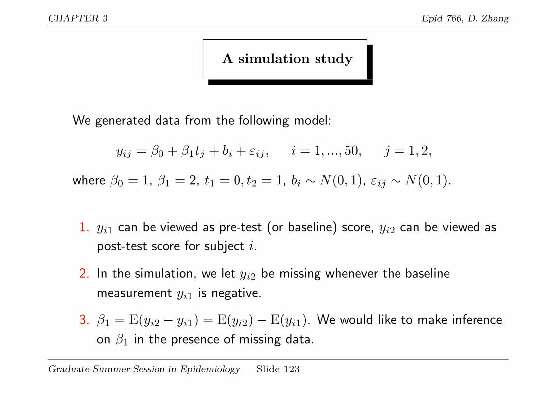
CHAPTER 3 Epid 766, D. Zhang
A simulation study
We generated data from the following model:
yij = β0 + β1tj + bi + εij , i = 1, ..., 50, j = 1, 2,
where β0 = 1, β1 = 2, t1 = 0, t2 = 1, bi ∼ N(0, 1), εij ∼ N(0, 1).
1. yi1 can be viewed as pre-test (or baseline) score, yi2 can be viewed as
post-test score for subject i.
2. In the simulation, we let yi2 be missing whenever the baseline
measurement yi1 is negative.
3. β1 = E(yi2 − yi1) = E(yi2)− E(yi1). We would like to make inference
on β1 in the presence of missing data.
Graduate Summer Session in Epidemiology Slide 123
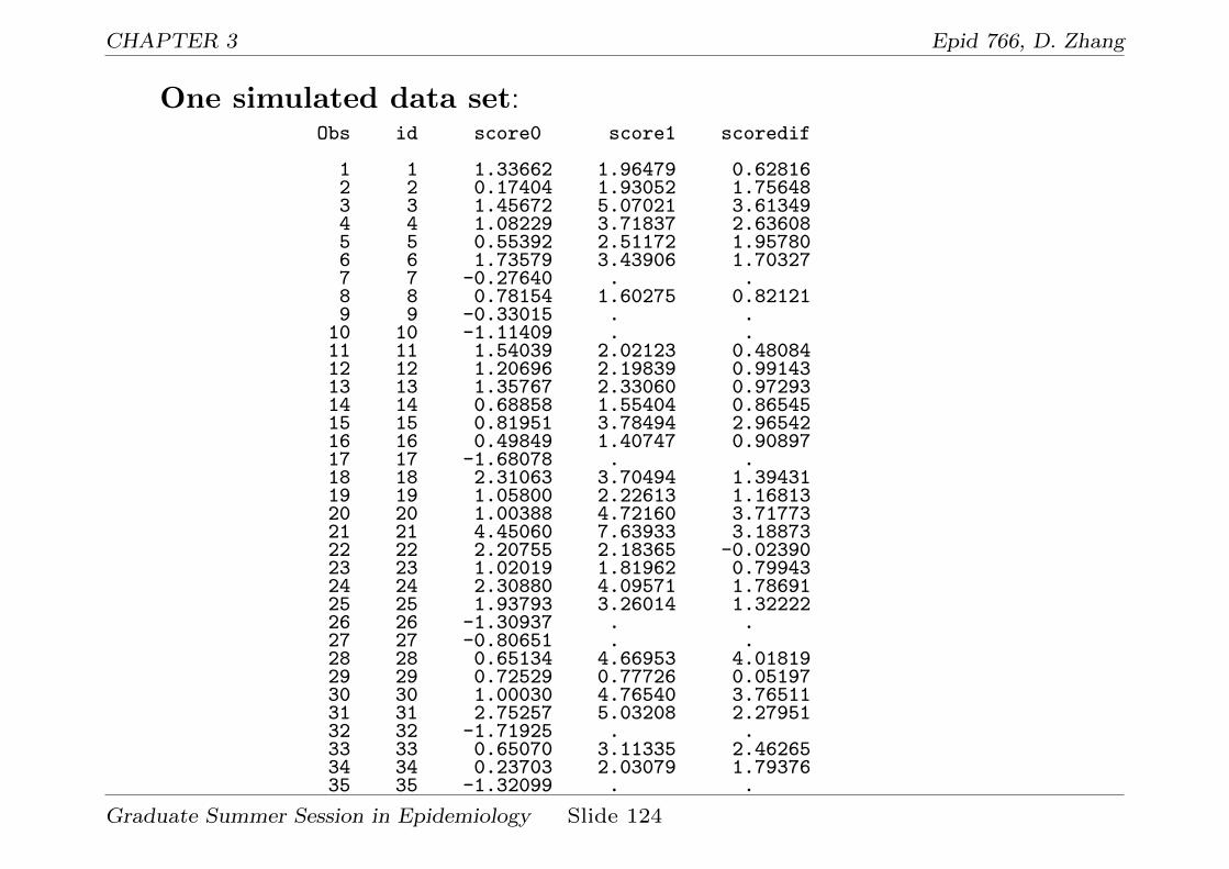
CHAPTER 3 Epid 766, D. Zhang
One simulated data set:Obs id score0 score1 scoredif
1 1 1.33662 1.96479 0.628162 2 0.17404 1.93052 1.756483 3 1.45672 5.07021 3.613494 4 1.08229 3.71837 2.636085 5 0.55392 2.51172 1.957806 6 1.73579 3.43906 1.703277 7 -0.27640 . .8 8 0.78154 1.60275 0.821219 9 -0.33015 . .
10 10 -1.11409 . .11 11 1.54039 2.02123 0.4808412 12 1.20696 2.19839 0.9914313 13 1.35767 2.33060 0.9729314 14 0.68858 1.55404 0.8654515 15 0.81951 3.78494 2.9654216 16 0.49849 1.40747 0.9089717 17 -1.68078 . .18 18 2.31063 3.70494 1.3943119 19 1.05800 2.22613 1.1681320 20 1.00388 4.72160 3.7177321 21 4.45060 7.63933 3.1887322 22 2.20755 2.18365 -0.0239023 23 1.02019 1.81962 0.7994324 24 2.30880 4.09571 1.7869125 25 1.93793 3.26014 1.3222226 26 -1.30937 . .27 27 -0.80651 . .28 28 0.65134 4.66953 4.0181929 29 0.72529 0.77726 0.0519730 30 1.00030 4.76540 3.7651131 31 2.75257 5.03208 2.2795132 32 -1.71925 . .33 33 0.65070 3.11335 2.4626534 34 0.23703 2.03079 1.7937635 35 -1.32099 . .
Graduate Summer Session in Epidemiology Slide 124
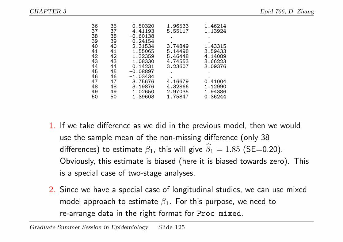
CHAPTER 3 Epid 766, D. Zhang
36 36 0.50320 1.96533 1.4621437 37 4.41193 5.55117 1.1392438 38 -0.60138 . .39 39 -0.24154 . .40 40 2.31534 3.74849 1.4331541 41 1.55065 5.14498 3.5943342 42 1.32359 5.46448 4.1408943 43 1.08330 4.74553 3.6622344 44 0.14231 3.23607 3.0937645 45 -0.08897 . .46 46 -1.03434 . .47 47 3.75676 4.16679 0.4100448 48 3.19876 4.32866 1.1299049 49 1.02650 2.97035 1.9438650 50 1.39603 1.75847 0.36244
1. If we take difference as we did in the previous model, then we would
use the sample mean of the non-missing difference (only 38
differences) to estimate β1, this will give β1 = 1.85 (SE=0.20).
Obviously, this estimate is biased (here it is biased towards zero). This
is a special case of two-stage analyses.
2. Since we have a special case of longitudinal studies, we can use mixed
model approach to estimate β1. For this purpose, we need to
re-arrange data in the right format for Proc mixed.
Graduate Summer Session in Epidemiology Slide 125

CHAPTER 3 Epid 766, D. Zhang
3. The data for the first 10 subjects are given below:Obs id score time
1 1 1.33662 02 1 1.96479 13 2 0.17404 04 2 1.93052 15 3 1.45672 06 3 5.07021 17 4 1.08229 08 4 3.71837 19 5 0.55392 0
10 5 2.51172 111 6 1.73579 012 6 3.43906 113 7 -0.27640 014 7 . 115 8 0.78154 016 8 1.60275 117 9 -0.33015 018 9 . 119 10 -1.11409 020 10 . 1
4. We use the following SAS program for estimating β1proc mixed data=maindat;
class id;model score = time / s;random int / subject=id type=vc;repeated / subject=id type=vc;
run;
Graduate Summer Session in Epidemiology Slide 126

CHAPTER 3 Epid 766, D. Zhang
5. Part of the output from the above SAS program:The Mixed Procedure
Model Information
Data Set WORK.MAINDATDependent Variable scoreCovariance Structure Variance ComponentsSubject Effects id, idEstimation Method REMLResidual Variance Method ParameterFixed Effects SE Method Model-BasedDegrees of Freedom Method Containment
Class Level Information
Class Levels Values
id 50 1 2 ..
Dimensions
Covariance Parameters 2Columns in X 2Columns in Z Per Subject 1Subjects 50Max Obs Per Subject 2Observations Used 88Observations Not Used 12Total Observations 100
Convergence criteria met.
Covariance Parameter Estimates
Graduate Summer Session in Epidemiology Slide 127

CHAPTER 3 Epid 766, D. Zhang
Cov Parm Subject Estimate
Intercept id 1.4573Residual id 0.7828
Fit Statistics
-2 Res Log Likelihood 300.6AIC (smaller is better) 304.6AICC (smaller is better) 304.8BIC (smaller is better) 308.4
The SAS System 5
The Mixed Procedure
Solution for Fixed Effects
StandardEffect Estimate Error DF t Value Pr > |t|
Intercept 0.9146 0.2117 49 4.32 <.0001time 2.0503 0.1987 37 10.32 <.0001
Type 3 Tests of Fixed Effects
Num DenEffect DF DF F Value Pr > F
time 1 37 106.50 <.0001
Graduate Summer Session in Epidemiology Slide 128

CHAPTER 3 Epid 766, D. Zhang
• The following table gives the simulation results comparing the
longitudinal approach modeling all responses simultaneously and the
two-stage approach modeling the difference based on 1000 simulation
runs:
Method Mean SE SD Cov. prob.
Longitudinal approach 2.002 0.222 0.257 0.91
Two-stage approach 1.712 0.214 0.217 0.72
where Mean is the sample mean of 1000 β1’s from both approaches; SE
is the sample mean of 1000 estimated SEs of β1; SD is the sample
standard deviation of 1000 β1’s; Cov. prob. is the empirical coverage
probability of 95% CI of β1.
Graduate Summer Session in Epidemiology Slide 129

CHAPTER 3 Epid 766, D. Zhang
What we see from this table:
1. The estimate β1 using longitudinal approach by modeling all responses
simultaneously is unbiased; however, if we take difference of the
responses (here we are forced to delete all subjects with missing
measurements), the estimate β1 is biased.
2. Although the estimate β1 from the two-stage approach has slightly
smaller SE or SD, since the estimate itself is biased, the coverage
probability of the 95% CI of β1 is too low, making invalid inference on
β1. However, the coverage probability of the 95% CI of β1 from the
longitudinal approach is almost right at the nominal level (0.95).
3. With mixed model approach, we can estimate other quantities.
Graduate Summer Session in Epidemiology Slide 130

CHAPTER 3 Epid 766, D. Zhang
3.4 Design a longitudinal study: Sample size
estimation
Recall that in the classical setting, sample size estimation is posed as a
hypothesis testing problem such as the following one
H0 : µ1 = µ2 vs HA : µ1 6= µ2.
Assume y1k, ..., ymk ∼ N(µk, σ2), k = 1, 2. Given significance level α,
power γ, and the difference ∆ = (µ1 − µ2)/σ we wish to detect, the
required total sample size (number of subjects) in each group should be
m = 2
[zα/2 + z1−γ
∆
]2.
Graduate Summer Session in Epidemiology Slide 131
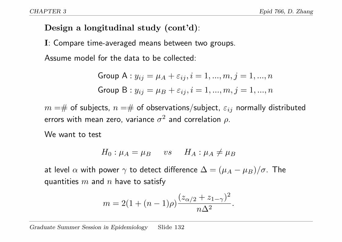
CHAPTER 3 Epid 766, D. Zhang
Design a longitudinal study (cont’d):
I: Compare time-averaged means between two groups.
Assume model for the data to be collected:
Group A : yij = µA + εij , i = 1, ...,m, j = 1, ..., n
Group B : yij = µB + εij , i = 1, ...,m, j = 1, ..., n
m =# of subjects, n =# of observations/subject, εij normally distributed
errors with mean zero, variance σ2 and correlation ρ.
We want to test
H0 : µA = µB vs HA : µA 6= µB
at level α with power γ to detect difference ∆ = (µA − µB)/σ. The
quantities m and n have to satisfy
m = 2(1 + (n− 1)ρ)(zα/2 + z1−γ)2
n∆2.
Graduate Summer Session in Epidemiology Slide 132

CHAPTER 3 Epid 766, D. Zhang
Comments:
1. When n = 1, the study reduces to a cross-sectional study and the
sample size formula reduces to the classical one.
2. When ρ = 0 (responses are independent), the required sample size is
1/n of that for classical study.
3. When ρ = 1, required sample size is the same as that of the classical
study.
4. For fixed n, smaller ρ gives smaller sample size.
5. If correlation is high, use more subjects and less obs/subject; if
correlation is low, use less subjects and more obs/subject.
6. The sample size formula depends on information on σ2 and ρ.
7. One can choose a combination of m and n to meet one’s specific
needs.
8. The above formula is for two-sided test.
Graduate Summer Session in Epidemiology Slide 133

CHAPTER 3 Epid 766, D. Zhang
• An example: If n = 3, α = 0.05, γ = 0.8, then the number of subjects
(m) per group is
m = 2(1 + 2ρ)(1.96 + 0.84)2
3∆2
∆
ρ 0.1 0.2 0.3 0.4 0.5 0.6 0.7 0.8
0.2 733 184 82 46 30 21 15 12
0.3 838 210 94 53 34 24 18 14
0.4 942 236 105 59 38 27 20 15
0.5 1047 262 117 66 42 30 22 17
0.6 1152 288 128 72 47 32 24 18
0.7 1256 314 140 79 51 35 26 20
0.8 1361 341 152 86 55 38 28 22
Graduate Summer Session in Epidemiology Slide 134

CHAPTER 3 Epid 766, D. Zhang
Design a longitudinal study (cont’d):
II: Compare slopes between two groups.
Model for the data to be collected:
Group A : yij = β0A + β1Atj + εij , i = 1, ...,m, j = 1, ..., n
Group B : yij = β0B + β1Btj + εij , i = 1, ...,m, j = 1, ..., n
m =# of subjects, n =# of observations/subject, εij are normal errors
with mean zero, variance σ2 and correlation ρ.
We are interested in testing
H0 : β1A = β1B vs HA : β1A 6= β1B
at level α with power γ to detect difference ∆ = (β1A − β1B)/σ. The
quantities m and n have to satisfy
m =2(1− ρ)(zα/2 + z1−γ)2
n∆2s2t, s2t =
∑nj=1(tj − t)2
n.
Graduate Summer Session in Epidemiology Slide 135

CHAPTER 3 Epid 766, D. Zhang
Comments:
1. For fixed time points tj , larger ρ gives smaller sample size m.
2. If ρ = 1, one subject from each group is enough.
3. ρ = 0 will require maximum sample size m.
4. If correlation is low, use more subjects and less obs/subject; if
correlation is high, use less subjects and more obs/subject.
5. The sample size formula depends on information on σ2 and ρ and the
placement of time points tj ’s.
6. One can choose a combination of m and n to meet one’s specific
needs.
7. The above formula is for two-sided test.
Graduate Summer Session in Epidemiology Slide 136

CHAPTER 3 Epid 766, D. Zhang
• An example: If n = 3, α = 0.05, γ = 0.8, t = (0, 2, 5) so s2t = 4.222,
then the number of subjects (m) per group is
m =2(1− ρ)(1.96 + 0.84)2
3× 4.222∆2
∆
ρ 0.02 0.03 0.04 0.05 0.06 0.07 0.08 0.09 0.10
0.2 2479 1102 620 397 276 203 155 123 100
0.3 2169 964 543 348 241 178 136 108 87
0.4 1859 827 465 298 207 152 117 92 75
0.5 1550 689 388 248 173 127 97 77 62
0.6 1240 551 310 199 138 102 78 62 50
0.7 930 414 233 149 104 76 59 46 38
0.8 620 276 155 100 69 51 39 31 25
Graduate Summer Session in Epidemiology Slide 137

CHAPTER 4 Epid 766, D. Zhang
4 Modeling discrete longitudinal data
• Generalized estimating equations (GEEs)
1. Why GEEs?
2. Key features of GEEs
3. Some popular GEE models
4. Some basics of GEEs
5. Interpretation of GEEs
6. Analyze infectious disease data using GEE
7. Analyze epileptic data using GEE
• Generalized linear mixed models (GLMMs)
1. Model specification & implementation
2. Analyze infectious disease data using a GLMM
3. Analyze epileptic data using a GLMM
Graduate Summer Session in Epidemiology Slide 138

CHAPTER 4 Epid 766, D. Zhang
4.1 Generalized estimating equations (GEEs) for
continuous and discrete longitudinal data
4.1.1 Why GEEs?
• Recall that a linear mixed model for longitudinal data may take the
form:
yij = β0 + β1tij + β2xij2 + · · ·+ βpxijp + bi0 + bi1tij + εij .
• Key features:
1. Outcome yij is continuous and normally distributed.
2. Correlation in outcome observations from the same individuals is
directly modeled using random effects (e.g., random intercept and
slope).
• However,
1. in many biomedical studies, the outcome variables are discrete (not
Graduate Summer Session in Epidemiology Slide 139

CHAPTER 4 Epid 766, D. Zhang
continuous). For example, the outcome is binary (yes/no) in
Indonesian children study, and the outcome is count in the Epileptic
clinical trial.
2. sometimes, we are mainly interested in the covariate effects, not in
correlation among the outcome observations from the same subject.
A partial reason is that it is much harder to know how the discrete
observations are correlated to each other over time than continuous
outcomes.
3. we might also want to model the correlation in a natural way jointly
with the estimation of covariate effects of interest.
Graduate Summer Session in Epidemiology Slide 140

CHAPTER 4 Epid 766, D. Zhang
What is wrong with the classical regression approach such as
the logistic regression for binary outcomes?
• Classical logistic regression model:
yi ∼ Binomial(1, πi(xi)), yi = 1/0, πi(xi) = E[yi|xi]
logit{πi(xi)} = log
{πi(xi)
1− πi(xi)
}= β0 + β1xi1 + · · ·+ βpxip.
• Key features:
1. Each subject contributes only one binary observation.
2. It is reasonable to assume that the outcomes from different subjects
are independent.
• However, in a longitudinal study,
1. Each subject has multiple binary (1/0) responses over time.
2. The subjects with higher probability to get disease will tend to have
more 1’s, resulting a correlation.
3. Even though a classical regression by ignoring correlation will giveGraduate Summer Session in Epidemiology Slide 141
CHAPTER 4 Epid 766, D. Zhang
us correct and meaningful regression coefficient estimates, their SEs
are often too small, resulting invalid inference.
4. The correlation has to be taken into account for valid inference (to
get correct standard errors of the regression coefficient estimates).
• Generalized estimating equations (GEEs) is an approach that
allows us to make valid inference by implicitly taken into account the
correlation.
Graduate Summer Session in Epidemiology Slide 142

CHAPTER 4 Epid 766, D. Zhang
4.1.2 Key features of GEEs for analyzing longitudinal data
1. We only need to correctly specify how the mean of the outcome
variable is related to the covariates of interest. For example, for the
infection disease study,
yij ∼ Binomial{1, πij(xij)}logit{πij(xij)} = β0 + β1Xeroij + β2sinvij + β3agei
+β4timeij + β5sexi + β6heightij ,
πij(xij) = P [yij = 1|xij ] = E(yij |xij) is the population
probability of respiratory infection for the population defined by the
specific covariate values (i.e., xij).
2. The correlation among the observations from the same subject over
time is not the major interest and is treated as nuisance.
3. We can specify a correlation structure. The validity of the inference
does not depend on the whether or not the specification of the
Graduate Summer Session in Epidemiology Slide 143

CHAPTER 4 Epid 766, D. Zhang
correlation structure is correct. GEE will give us a robust inference on
the regression coefficients, which is valid regardless whether or not the
correlation structure we specified is right.
4. GEE calculates correct SEs for the regression coefficient estimates
using sandwich estimates that will take into account the possibility
that the correlation structure is misspecified.
5. The regression coefficients in GEE have a population-average
interpretation.
6. A fundamental assumption on missing data is that missing data
mechanism has to be MCAR, while a likelihood-based approach only
requires MAR. The GEE approach will also be less efficient than a
likelihood-based approach if the likelihood can be correctly specified.
Graduate Summer Session in Epidemiology Slide 144

CHAPTER 4 Epid 766, D. Zhang
4.1.3 Some popular GEE Models
• Continuous (Normal):
µ(x) = β0 + β1x1 + · · ·+ βpxp
where µ(x) = E(y|x) is the mean of outcome variable at
x = (x1, ..., xp), such as mean of cholesterol level.
• Proportion (Binomial, Binary):
logit{π(x)} = β0 + β1x1 + · · ·+ βpxp
π(x) = P [y = 1|x] = E(y|x) such as disease risk.
logit(π) = log{π/(1− π)} is the logit link function. Other link
functions are possible.
Graduate Summer Session in Epidemiology Slide 145
CHAPTER 4 Epid 766, D. Zhang
• Count or rate (Poisson-type)
log{λ(x)} = β0 + β1x1 + · · ·+ βpxp
λ(x) is the rate (e.g. λ(x) is the incidence rate of a disease) for the
count data (number of events) y over a (time, space) region T such
that
y|x ∼ Poisson{λ(x)T}
Here log(.) link is used. Other link functions are possible.
Note: For count data, we have to be concerned about the possible
over-dispersion in the data. That is
var(y|x) > E(y|x).
One way to model this phenomenon is to use an over-dispersion
parameter φ and model the variance-mean relationship as follows:
var(y|x) = φE(y|x).
Graduate Summer Session in Epidemiology Slide 146

CHAPTER 4 Epid 766, D. Zhang
4.1.4 Some basics of GEEs
• Data: yij , i = 1, ...,m, j = 1, ..., ni with mean
µij = E(yij |xij).
Denote
yi =
yi1
yi2...
yini
, µi =
µi1
µi2...
µini
.
• Suppose we correctly specify the mean structure for data yij :
g(µij) = β0 + x1ijβ1 + ...+ xpijβp,
where g(µ) is the link function such as the logit function for binary
response and the log link for count data.
Graduate Summer Session in Epidemiology Slide 147

CHAPTER 4 Epid 766, D. Zhang
• A GEE solves the following generalized estimating equation for β
(Liang and Zeger, 1986):
Sβ(α, β) =m∑i=1
(∂µi∂β
)TV −1i (yi − µi) = 0, (4.1)
where Vi is some matrix (intended to specify for var(yi|xi)) and α is
the possible parameters in the correlation structure.
• The above estimating equation is unbiased no matter what matrix Vi
we use as long as the mean structure is right. That is
E[Sβ(α, β)] = 0.
• Under some regularity conditions, the solution β from the GEE
equation (4.1) has asymptotic distribution
βa∼ N(β,Σ),
Graduate Summer Session in Epidemiology Slide 148

CHAPTER 4 Epid 766, D. Zhang
where
Σ = I−10 I1I−10
I0 =
m∑i=1
DTi V−1i Di
I1 =
m∑i=1
DTi V−1i var(yi|xi)V −1i Di
=m∑i=1
DTi V−1i (yi − µi(β))(yi − µi(β))TV −1i Di
Σ is called the empirical, robust or sandwich variance estimate.
• If Vi is correctly specified, then I1 ≈ I0 and Σ ≈ I−10 (model based).
In this case, β is the most efficient estimate. Otherwise, Σ 6= I−10 .
Graduate Summer Session in Epidemiology Slide 149

CHAPTER 4 Epid 766, D. Zhang
• Vi, the working variance matrix for yi (at xi), can be decomposed as
Vi = A1/2i RiA
1/2i ,
where
Ai =
var(yi1|xi1) 0 · · · 0
0 var(yi2|xi2) · · · 0...
......
...
0 · · · 0 var(yini|xini
)
,
and Ri is the correlation structure.
• We may try to specify Ri so that it is close to the “true”. This Ri is
called the working correlation matrix and may be mis-specified.
Graduate Summer Session in Epidemiology Slide 150
CHAPTER 4 Epid 766, D. Zhang
• Some working correlation structures
1. Independent: Ri(α) = Ini×ni . No α needs to be estimated.
2. Exchangeable (compound symmetric):
Ri =
1 α · · · α
α 1 · · · α...
......
...
α α · · · 1
Let eij = yij − µij . Since E(eijeik) = φα (at true β), =⇒
α =1
(N∗ − p− 1)φ
m∑i=1
∑j<k
eijeik,
where N∗ =∑mi=1 ni(ni − 1)/2 (total # of pairs), φ is usually
estimated using the Pearson χ2.
Graduate Summer Session in Epidemiology Slide 151

CHAPTER 4 Epid 766, D. Zhang
3. AR(1):
Ri =
1 α · · · αni−1
α 1 · · · αni−2
......
......
αni−1 αni−2 · · · 1
Since E(eijei,j+1) = φα (at true β), =⇒
α =1
(N∗∗ − p− 1)φ
m∑i=1
ni−1∑j=1
eijei,j+1,
where N∗∗ =∑mi=1(ni − 1) (total # of adjacent pairs).
4. Many more can be found in SAS.
• Software: Proc Genmod in SAS
Graduate Summer Session in Epidemiology Slide 152

CHAPTER 4 Epid 766, D. Zhang
4.1.5 Interpretation of regression coefficients in a GEE Model
• A classical logistic model: y = indicator of lung cancer ∼ Bin(1, π)
logit(π) = β0 + β1XE + β2XC
where
XE =
1 exposure = yes
0 exposure = noXC =
1 confounder = yes
0 confounder = no
For example, XE = smoking (yes/no), XC = Age (> 50 vs. ≤ 50).
Then
β1 = age-adjusted log(OR) (≈ log(RR)) of lung cancer comparing the
population of smokers and the population of non-smokers.
Graduate Summer Session in Epidemiology Slide 153
CHAPTER 4 Epid 766, D. Zhang
• In general, βk in a logistic regression can be interpreted as
βk = log(OR) of disease under consideration for two populations with
covariate values xk + 1 and xk while other covariates are held fixed.
• The regression coefficients in a GEE logistic model have the same
population-averaged interpretation as those in a classical logistic
model.
• GEE combines information from a sample of subjects to estimate these
population-averaged estimates. These will be contrasted with
subject-specific regression coefficients later.
Graduate Summer Session in Epidemiology Slide 154

CHAPTER 4 Epid 766, D. Zhang
4.1.6 Analyze Infectious disease data using GEE
• Data:
? 275 Indonesian preschool children.
? Each was followed over 6 consecutive quarters.
? Outcome = respiratory infection (yes/no)
? Covariates: Xero (xerophthalmia (yes/no)), season, age, sex, height
(height for age)
• GEE logistic model: yij(1/0) = infection indicator ∼ Bin(1, πij),
logit(πij) = β0 + β1Xeroij + β2sinvij + β3agei
+β4timeij + β5sexi + β6heightij
See the SAS program indon gee.sas and its output indon gee.lst
for details.
Graduate Summer Session in Epidemiology Slide 155

CHAPTER 4 Epid 766, D. Zhang
SAS program: indon gee.sas
options ls=72 ps=72;
/*------------------------------------------------------*//* *//* Proc Genmod to fit population average (marginal) *//* model using GEE approach for the Indonesia children *//* infection disease data *//* *//*------------------------------------------------------*/
data indon;infile "indon.dat";input id infect intercept age xero cosv sinv sex height stuntedvisit baseage season visitsq;time = age-baseage;/* sinv = sin(season*8*atan(1)/4); */
run;
data indon; set indon;nobs=_n_;
run;
title "Print the first 20 observations";proc print data=indon (obs=20);
var id infect xero sex visit season;run;
title "Model 1: Use exchangeable working correlation";proc genmod descending;class id;model infect = xero sinv baseage time sex height
/ dist=bin link=logit;repeated subject=id / type=exch corrw;
run;
Graduate Summer Session in Epidemiology Slide 156

CHAPTER 4 Epid 766, D. Zhang
SAS first uses indep. corr to obtain reg parm est:
Analysis Of Initial Parameter Estimates
Standard Wald 95% Chi-Parameter DF Estimate Error Confidence Limits Square Pr > ChiSq
Intercept 1 -2.4708 0.2122 -2.8867 -2.0549 135.59 <.0001xero 1 0.6661 0.4343 -0.1852 1.5174 2.35 0.1251sinv 1 -0.0640 0.1517 -0.3613 0.2333 0.18 0.6730baseage 1 -0.0335 0.0064 -0.0461 -0.0209 27.22 <.0001time 1 0.0000 0.0200 -0.0392 0.0392 0.00 0.9999sex 1 -0.3841 0.2188 -0.8129 0.0448 3.08 0.0792height 1 -0.0476 0.0207 -0.0882 -0.0070 5.29 0.0215
Actual SAS output from the above program:
Model 1: Use exchangeable working correlation 2
The GENMOD Procedure
Model Information
Data Set WORK.INDONDistribution BinomialLink Function LogitDependent Variable infect
Number of Observations Read 1200Number of Observations Used 1200Number of Events 107Number of Trials 1200
Graduate Summer Session in Epidemiology Slide 157

CHAPTER 4 Epid 766, D. Zhang
Class Level Information
Class Levels Values
id 275 121013 121113 121114 121140 121215 121315 121316121413 121414 121514 121616 121617 121713 121813121913 122013 122113 122114 122170 122214 122315124150 124160 125140 127130 128130 129130 129140131015 131016 131116 131140 131215 131216 131315131417 ...
Response Profile
Ordered TotalValue infect Frequency
1 1 1072 0 1093
PROC GENMOD is modeling the probability that infect=’1’.
Parameter Information
Parameter Effect
Prm1 InterceptPrm2 xeroPrm3 seasonPrm4 baseagePrm5 timePrm6 sexPrm7 height
Algorithm converged.
Graduate Summer Session in Epidemiology Slide 158

CHAPTER 4 Epid 766, D. Zhang
GEE Model Information
Correlation Structure ExchangeableSubject Effect id (275 levels)Number of Clusters 275Correlation Matrix Dimension 6Maximum Cluster Size 6Minimum Cluster Size 1
Algorithm converged.
Working Correlation Matrix
Col1 Col2 Col3 Col4 Col5 Col6
Row1 1.0000 0.0460 0.0460 0.0460 0.0460 0.0460Row2 0.0460 1.0000 0.0460 0.0460 0.0460 0.0460Row3 0.0460 0.0460 1.0000 0.0460 0.0460 0.0460Row4 0.0460 0.0460 0.0460 1.0000 0.0460 0.0460Row5 0.0460 0.0460 0.0460 0.0460 1.0000 0.0460Row6 0.0460 0.0460 0.0460 0.0460 0.0460 1.0000
Exchangeable WorkingCorrelation
Correlation 0.0459822403
GEE Fit Criteria
QIC 700.6732QICu 699.4715
Graduate Summer Session in Epidemiology Slide 159

CHAPTER 4 Epid 766, D. Zhang
Analysis Of GEE Parameter EstimatesEmpirical Standard Error Estimates
Standard 95% ConfidenceParameter Estimate Error Limits Z Pr > |Z|
Intercept -2.4592 0.2250 -2.9002 -2.0181 -10.93 <.0001xero 0.5529 0.4479 -0.3249 1.4308 1.23 0.2170sinv -0.0575 0.1146 -0.2822 0.1672 -0.50 0.6158baseage -0.0339 0.0062 -0.0460 -0.0218 -5.50 <.0001time 0.0010 0.0210 -0.0401 0.0421 0.05 0.9614sex -0.4000 0.2374 -0.8654 0.0653 -1.68 0.0920height -0.0509 0.0262 -0.1024 0.0005 -1.94 0.0524
Graduate Summer Session in Epidemiology Slide 160

CHAPTER 4 Epid 766, D. Zhang
Some remarks:
• Proc Genmod in SAS fits the model using independence correlation
structure to get initial parameter estimate and get the estimate of
over-dispersion parameter (SAS does not output the initial estimates
now). We should read the output under “Analysis Of GEE
Parameter Estimates”, which is valid even if the correlation
structure we specified (it is exchangeable here) may not be true.
• Given other characteristics, the odds-ratio of getting respiratory
infection between two populations with or without Vitamin A
deficiency is estimated to be e0.5529 = 1.74. If respiratory infection
could be viewed as a rare disease, kids with Vitamin A deficiency would
be 74% more likely to develop respiratory infection. However,
p-value=0.2170 indicates that there is no significant difference in
infection risk for these two populations.
Graduate Summer Session in Epidemiology Slide 161

CHAPTER 4 Epid 766, D. Zhang
4.1.7 Analyze epileptic seizure count data using GEE
• Data:
? 59 patients, 28 in control group, 31 in treatment (progabide) group.
? 5 seizure counts (including baseline) were obtained.
? Covariates: treatment (covariate of interest), age.
• GEE Poisson model: yij =seizure counts obtained at the jth
(j = 1, 2, ..., 5) time point for patient i, yij ∼ over-dispersed
Poisson(µij), µij = E(yij) = tijλij , where tij is the length of time
from which the seizure count yij was observed, λij is hence the rate to
have a seizure. First consider model
log(λij) = β0 + β1I(j > 1) + β2trti + β3trtiI(j > 1)
log(µij) = log(tij) + β0 + β1I(j > 1) + β2trti + β3trtiI(j > 1)
Note that log(tij) is often called an offset.
Graduate Summer Session in Epidemiology Slide 162

CHAPTER 4 Epid 766, D. Zhang
• Interpretation of β’s:
log of seizure rate λ
Group Before RAND (j = 1) After RAND (j > 1)
Control (trt=0) β0 β0 + β1
Treatment (trt=1) β0 + β2 β0 + β1 + β2 + β3
Therefore, β1 = time and placebo effect, β2 = difference in seizure
rates at baseline between two groups, β3 = treatment effect of interest
(accounting for time & placebo effect).
If randomization is taken into account (β2 = 0), we can consider the
following model
log(µij) = log(tij) + β0 + β1I(j > 1) + β2trtiI(j > 1)
• See the SAS program seize gee.sas and its output seize gee.lst
for details.
Graduate Summer Session in Epidemiology Slide 163

CHAPTER 4 Epid 766, D. Zhang
First part of seize gee.sas
options ls=80 ps=1000 nodate;
/*------------------------------------------------------*//* *//* Proc Genmod to fit population average (marginal) *//* model using GEE approach for the epileptic seizure *//* count data *//* *//*------------------------------------------------------*/
data seizure;infile "seize.dat";input id seize visit trt age;nobs=_n_;interval = 2;if visit=0 then interval=8;logtime = log(interval);assign = (visit>0);
run;
title "Model 1: overall effect of the treatment";proc genmod data=seizure;
class id;model seize = assign trt assign*trt
/ dist=poisson link=log offset=logtime;repeated subject=id / type=exch corrw;
run;
Graduate Summer Session in Epidemiology Slide 164

CHAPTER 4 Epid 766, D. Zhang
SAS first uses indep corr to get reg. coeff est.
Analysis Of Initial Parameter Estimates
Standard Wald 95% Chi-Parameter DF Estimate Error Confidence Limits Square Pr > ChiSq
Intercept 1 1.3476 0.0341 1.2809 1.4144 1565.44 <.0001assign 1 0.1108 0.0469 0.0189 0.2027 5.58 0.0181trt 1 0.0265 0.0467 -0.0650 0.1180 0.32 0.5702assign*trt 1 -0.1037 0.0651 -0.2312 0.0238 2.54 0.1110
Actual SAS output from the above program:
Model 1: overall effct of the treatment 1
The GENMOD Procedure
Model Information
Data Set WORK.SEIZUREDistribution PoissonLink Function LogDependent Variable seizeOffset Variable logtime
Number of Observations Read 295Number of Observations Used 295
Class Level Information
Class Levels Values
id 59 101 102 103 104 106 107 108 110 111 112 113 114116 117 118 121 122 123 124 126 128 129 130 135
Graduate Summer Session in Epidemiology Slide 165

CHAPTER 4 Epid 766, D. Zhang
137 139 141 143 145 147 201 202 203 204 205 206207 208 209 210 211 213 214 215 217 218 219 220221 222 225 226 227 228 230 232 234 236 238
Parameter Information
Parameter Effect
Prm1 InterceptPrm2 assignPrm3 trtPrm4 assign*trt
Algorithm converged.
GEE Model Information
Correlation Structure ExchangeableSubject Effect id (59 levels)Number of Clusters 59Correlation Matrix Dimension 5Maximum Cluster Size 5Minimum Cluster Size 5
Algorithm converged.
Working Correlation Matrix
Col1 Col2 Col3 Col4 Col5
Row1 1.0000 0.7716 0.7716 0.7716 0.7716Row2 0.7716 1.0000 0.7716 0.7716 0.7716Row3 0.7716 0.7716 1.0000 0.7716 0.7716Row4 0.7716 0.7716 0.7716 1.0000 0.7716Row5 0.7716 0.7716 0.7716 0.7716 1.0000
Graduate Summer Session in Epidemiology Slide 166

CHAPTER 4 Epid 766, D. Zhang
Exchangeable WorkingCorrelation
Correlation 0.7715879669
GEE Fit Criteria
QIC -659.5869QICu -668.6570
Analysis Of GEE Parameter EstimatesEmpirical Standard Error Estimates
Standard 95% ConfidenceParameter Estimate Error Limits Z Pr > |Z|
Intercept 1.3476 0.1574 1.0392 1.6560 8.56 <.0001assign 0.1108 0.1161 -0.1168 0.3383 0.95 0.3399trt 0.0265 0.2219 -0.4083 0.4613 0.12 0.9049assign*trt -0.1037 0.2136 -0.5223 0.3150 -0.49 0.6274
Graduate Summer Session in Epidemiology Slide 167

CHAPTER 4 Epid 766, D. Zhang
Second part of seize gee.sas
title "Model 2: take randomization into account";proc genmod data=seizure;
class id;model seize = assign assign*trt
/ dist=poisson link=log offset=logtime scale=pearson aggregate=nobs;repeated subject=id / type=exch corrw;
run;
Output from the above program:
Model 2: take randomization into account 2
Algorithm converged.
Working Correlation Matrix
Col1 Col2 Col3 Col4 Col5
Row1 1.0000 0.7750 0.7750 0.7750 0.7750Row2 0.7750 1.0000 0.7750 0.7750 0.7750Row3 0.7750 0.7750 1.0000 0.7750 0.7750Row4 0.7750 0.7750 0.7750 1.0000 0.7750Row5 0.7750 0.7750 0.7750 0.7750 1.0000
Exchangeable WorkingCorrelation
Correlation 0.7749556223
GEE Fit Criteria
QIC -667.9355QICu -672.7671
Graduate Summer Session in Epidemiology Slide 168

CHAPTER 4 Epid 766, D. Zhang
Analysis Of GEE Parameter EstimatesEmpirical Standard Error Estimates
Standard 95% ConfidenceParameter Estimate Error Limits Z Pr > |Z|
Intercept 1.3616 0.1111 1.1438 1.5794 12.25 <.0001assign 0.1173 0.1283 -0.1341 0.3688 0.91 0.3604assign*trt -0.1170 0.2076 -0.5240 0.2900 -0.56 0.5731
Graduate Summer Session in Epidemiology Slide 169

CHAPTER 4 Epid 766, D. Zhang
A program to adjust for age
title "Model 3: adjusting for other covariates (age)";proc genmod data=seizure;
class id;model seize = assign trt assign*trt age
/ dist=poisson link=log offset=logtime scale=pearson;repeated subject=id / type=exch corrw;
run;
Output of the program to adjust for all covariates
Model 3: adjusting for other covariates 3
Algorithm converged.
Working Correlation Matrix
Col1 Col2 Col3 Col4 Col5
Row1 1.0000 0.7620 0.7620 0.7620 0.7620Row2 0.7620 1.0000 0.7620 0.7620 0.7620Row3 0.7620 0.7620 1.0000 0.7620 0.7620Row4 0.7620 0.7620 0.7620 1.0000 0.7620Row5 0.7620 0.7620 0.7620 0.7620 1.0000
Exchangeable WorkingCorrelation
Correlation 0.7620401547
GEE Fit Criteria
QIC -686.4053QICu -697.2349
Graduate Summer Session in Epidemiology Slide 170

CHAPTER 4 Epid 766, D. Zhang
Analysis Of GEE Parameter EstimatesEmpirical Standard Error Estimates
Standard 95% ConfidenceParameter Estimate Error Limits Z Pr > |Z|
Intercept 2.2601 0.4330 1.4113 3.1088 5.22 <.0001assign 0.1108 0.1161 -0.1168 0.3383 0.95 0.3399trt -0.0175 0.2141 -0.4371 0.4020 -0.08 0.9348assign*trt -0.1037 0.2136 -0.5223 0.3150 -0.49 0.6274age -0.0321 0.0147 -0.0610 -0.0032 -2.17 0.0296
Graduate Summer Session in Epidemiology Slide 171

CHAPTER 4 Epid 766, D. Zhang
4.2 Generalized linear mixed models (GLMMs)
4.2.1 Model specification and implementation
• Generalized linear mixed models (GLMMs) are an extension of
1. linear mixed models (continuous ⇒ discrete)
2. logistic (Poisson) models (independent discrete data ⇒discrete longitudinal data)
• Consider a special linear mixed model:
yij = β0 + β1xij1 + · · ·+ βpxijp + bi + εij ,
where bi ∼ N(0, σ2b ) and εij
iid∼ N(0, σ2ε).
Let µbij = E[yij |bi]. Then the above model is equivalent to
yij |bi, xiind∼ N(µbij , σ
2ε),
µbij = β0 + β1xij1 + · · ·+ βpxijp + bi.(4.2)
Graduate Summer Session in Epidemiology Slide 172

CHAPTER 4 Epid 766, D. Zhang
• Extend above model (4.2) to logistic model for longitudinal binary
data:
yij |bi, xiind∼ Binomial{1, πbij(xi)},
logit{πbij(xi)} = log
{πbij(xi)
1−πbij(xi)
}= β0 + β1xij1 + · · ·+ βpxijp + bi
bi ∼ N(0, σ2b ),
(4.3)
where bi are the (normal) subject-specific random effects. This is a
special GLMM (logistic-normal).
• Remarks:
1. In this model the correlation is modeled through random effects bi.
A subject with higher bi will have higher disease probability πbij (if
other covariate values are kept the same).
2. Random effects bi vary from subject to subject and are assumed to
be independent. Hence the data {yij} from the same individuals
Graduate Summer Session in Epidemiology Slide 173
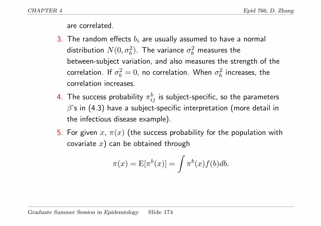
CHAPTER 4 Epid 766, D. Zhang
are correlated.
3. The random effects bi are usually assumed to have a normal
distribution N(0, σ2b ). The variance σ2
b measures the
between-subject variation, and also measures the strength of the
correlation. If σ2b = 0, no correlation. When σ2
b increases, the
correlation increases.
4. The success probability πbij is subject-specific, so the parameters
β’s in (4.3) have a subject-specific interpretation (more detail in
the infectious disease example).
5. For given x, π(x) (the success probability for the population with
covariate x) can be obtained through
π(x) = E[πb(x)] =
∫πb(x)f(b)db.
Graduate Summer Session in Epidemiology Slide 174

CHAPTER 4 Epid 766, D. Zhang
6. Even though πb(x) has a logistic form in model (4.3), π(x) does
NOT have a logistic form. In particular:
logit{π(x)} 6= β0 + β1x1 + · · ·+ βpxp.
7. However, approximately we have
logit{π(x)} ≈ (1+0.346σ2b )−1/2× (β0 +β1x1 + · · ·+βpxp). (4.4)
That is, (1 + 0.346σ2b )−1/2βk has a population-level interpretation
in terms of log odds-ratio.
Graduate Summer Session in Epidemiology Slide 175

CHAPTER 4 Epid 766, D. Zhang
• Extend above model (4.2) to log-linear model for longitudinal Poisson
(count) data:
yij |biind∼ Poisson(µbij = Tijλ
bij),
log(λbij) = β0 + β1xij1 + · · ·+ βpxijp + bi
log(µbij) = log(Tij) + β0 + β1xij1 + · · ·+ βpxijp + bi
bi ∼ N(0, σ2b ),
(4.5)
where bi are the (normal) subject-specific random effects. This is a
special GLMM (Poisson-normal).
• Remarks:
1. In this model, the correlation is modeled through random effects bi.
A subject with higher bi will have larger rate λbij (if other covariate
values are kept the same), and tend to have larger responses.
2. Random effects bi vary from subject to subject and are assumed to
be independent. Hence the data {yij} from the same individuals
are correlated.Graduate Summer Session in Epidemiology Slide 176

CHAPTER 4 Epid 766, D. Zhang
3. The random effects bi are usually assumed to have a normal
distribution N(0, σ2b ). The variance σ2
b measures the
between-subject variation, and also measures the strength of the
correlation. If σ2b = 0, no correlation. When σ2
b increases, the
correlation increases.
4. The event rate λbij is subject-specific, so the parameters β’s in (4.5)
have a subject-specific interpretation (more detail in the Epileptic
seizure count example).
5. There still may be overdispersion for yij |bi. That is
var(yij |bi) > E(yij |bi). So we may take the over-dispersion into
account by assuming
var(yij |bi) = φE(yij |bi).
Note: This φ is different from the φ in GEE.
Graduate Summer Session in Epidemiology Slide 177

CHAPTER 4 Epid 766, D. Zhang
? One way to account for overdispersion is to use statement
random residual in Proc Glimmix.
? The other way is to assume yij |bi has the following log
quasi-likelihood function:
`q(yij , µbij) =
yij(logµbij − log yij)− (µbij − yij)φ
− 1
2log φ.
? Or to assume yij |bi has a generalized Poisson distribution:
f(yij |bi) =(1− ξ)µbij{(1− ξ)µbij + ξyij}yij−1e−(1−ξ)µ
bij−ξyij
yij !.
In this case,
E(yij |bi) = µbij , var(yij |bi) = µbij/(1− ξ)2,
so over-dispersion parameter is 1/(1− ξ)2.
Graduate Summer Session in Epidemiology Slide 178

CHAPTER 4 Epid 766, D. Zhang
6. For given x, the population event rate λ(x) (the event rate for the
population with covariate x) can be obtained through
λ(x) = E[λb(x)]
= E[eβ0+β1x1+···+βpxp+b
]= eβ0+β1x1+···+βpxpE(eb)
= eβ0+β1x1+···+βpxpeσ2b/2
= eσ2b/2+β0+β1x1+···+βpxp
= eβ0+β1x1+···+βpxp
=⇒
log{λ(x)} = β0 + β1x1 + · · ·+ βpxp, (4.6)
therefore, the regression coefficients β’s (except β0) in model (4.5)
also have population average interpretation.
Graduate Summer Session in Epidemiology Slide 179

CHAPTER 4 Epid 766, D. Zhang
• For a liner mixed model like the following
yij = βTxij + bi0 + εij ,
where εijiid∼ N(0, σ2
ε ), we have
E(yij |bi) = βTxij + bi0 and E(yij) = βTxij .
So the β’s (except the intercept β0) always have population-averaged
interpretation as well as subject-specific interpretation.
Graduate Summer Session in Epidemiology Slide 180

CHAPTER 4 Epid 766, D. Zhang
• Why GLMMs?
1. We are interested in how the outcome variable is related to the
independent variables (covariates).
2. We are also interested in how individuals’ data vary from subject to
subject (between-subject variation). This can be modeled through
the use of random effects. The random effects have a natural
interpretation.
3. A GLMM is a likelihood-based model. So it requires much less
strong assumption for missing data mechanism. Only MAR
mechanism is required for a GLMM to make valid inference,
compared to MCAR for GEE approach.
4. The regression coefficients have a subject-specific interpretation,
and for some special GLMMs we can still (approximately) make
population level inference.
Graduate Summer Session in Epidemiology Slide 181

CHAPTER 4 Epid 766, D. Zhang
• Implementation: Proc Glimmix for GLMMs in SAS where
approximate integration is used for approximate or exact maximum
quasi-likelihood/likelihood estimation. Or Proc Nlmixed (non-linear
mixed model) in SAS where numerical integration is used for maximum
likelihood estimation.
Graduate Summer Session in Epidemiology Slide 182
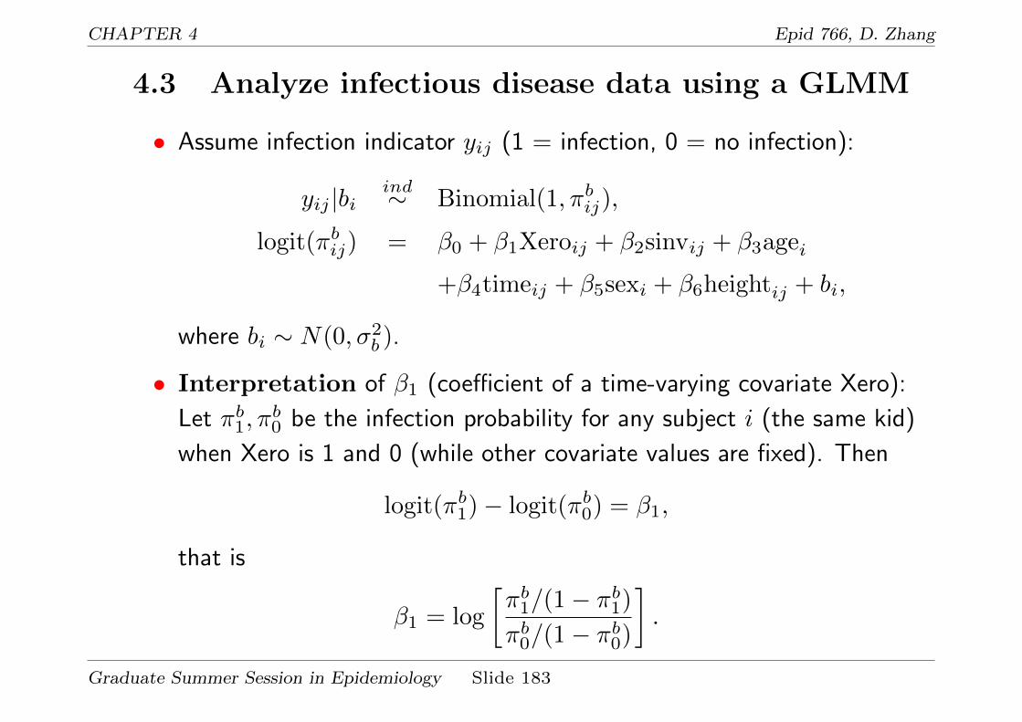
CHAPTER 4 Epid 766, D. Zhang
4.3 Analyze infectious disease data using a GLMM
• Assume infection indicator yij (1 = infection, 0 = no infection):
yij |biind∼ Binomial(1, πbij),
logit(πbij) = β0 + β1Xeroij + β2sinvij + β3agei
+β4timeij + β5sexi + β6heightij + bi,
where bi ∼ N(0, σ2b ).
• Interpretation of β1 (coefficient of a time-varying covariate Xero):
Let πb1, πb0 be the infection probability for any subject i (the same kid)
when Xero is 1 and 0 (while other covariate values are fixed). Then
logit(πb1)− logit(πb0) = β1,
that is
β1 = log
[πb1/(1− πb1)
πb0/(1− πb0)
].
Graduate Summer Session in Epidemiology Slide 183

CHAPTER 4 Epid 766, D. Zhang
That is, β1 is the log odds-ratio of getting respiratory infection if a
subject becomes Vitamin A deficiency (from Vitamin A sufficiency).
Similar interpretation holds for continuous time-varying covariates.
• Interpretation of β5 (coefficient of a one-time covariate sex): Let
πbi1 be the infection probability for subject i who is a boy and πbj0 be
the infection probability for subject j who is a girl. Assume they have
the same covariate values (except sex). Then
logit(πbi1 )− logit(πbj0 ) = β5 + (bi − bj).
If bi ≈ bj , then
logit(πbi1 )− logit(πbj0 ) ≈ β5,
β5 ≈ log
[πbi1 /(1− π
bi1 )
πbj0 /(1− π
bj0 )
].
That is, β5 is the log odds-ratio of getting respiratory infection
comparing a boy and a girl who are similar in other subject
characteristics except gender. Similar interpretation holds forGraduate Summer Session in Epidemiology Slide 184

CHAPTER 4 Epid 766, D. Zhang
continuous one-time covariates.
See the SAS program indon mix.sas and its output indon mix.lst
for details.
Graduate Summer Session in Epidemiology Slide 185

CHAPTER 4 Epid 766, D. Zhang
• Remark 1: As indicated by (4.4), (1 + 0.346σ2b )−1/2β have
population log odds-ratio interpretation:
logit(πij) ≈ (1 + 0.346σ2b )−1/2βTxij
= βTxij ,
where β = (1 + 0.346σ2b )−1/2β. Therefore, β has population-average
interpretation. That is, we can use β to compare two populations.
Graduate Summer Session in Epidemiology Slide 186

CHAPTER 4 Epid 766, D. Zhang
SAS program indon mix.sas
options ls=80 ps=1000 nodate;
/*------------------------------------------------------*//* *//* Proc Glimmix to fit subject-specific (random effect) *//* model for the Indonesian children infection disease *//* data *//* *//*------------------------------------------------------*/
data indon;infile "indon.dat";input id infect intercep age xero cosv sinv sex height stuntedvisit baseage season visitsq;time = age - baseage;
run;
title "Random intercept model for infection disease data";proc glimmix data=indon method=quad;
class id;model infect = xero sinv age time sex height / dist=bin link=logit s;random int / subject=id type=vc;
run;
Graduate Summer Session in Epidemiology Slide 187

CHAPTER 4 Epid 766, D. Zhang
SAS output indon mix.lst
Random intercept model for infection disease data 1
The GLIMMIX Procedure
Model Information
Data Set WORK.INDONResponse Variable infectResponse Distribution BinomialLink Function LogitVariance Function DefaultVariance Matrix Blocked By idEstimation Technique Maximum LikelihoodLikelihood Approximation Gauss-Hermite QuadratureDegrees of Freedom Method Containment
Class Level Information
Class Levels Values
id 275 121013 121113 121114 121140 121215 121315121316 ...
Number of Observations Read 1200Number of Observations Used 1200
Graduate Summer Session in Epidemiology Slide 188

CHAPTER 4 Epid 766, D. Zhang
Dimensions
G-side Cov. Parameters 1Columns in X 7Columns in Z per Subject 1Subjects (Blocks in V) 275Max Obs per Subject 6
Optimization Information
Optimization Technique Dual Quasi-NewtonParameters in Optimization 8Lower Boundaries 1Upper Boundaries 0Fixed Effects Not ProfiledStarting From GLM estimatesQuadrature Points 9
Graduate Summer Session in Epidemiology Slide 189
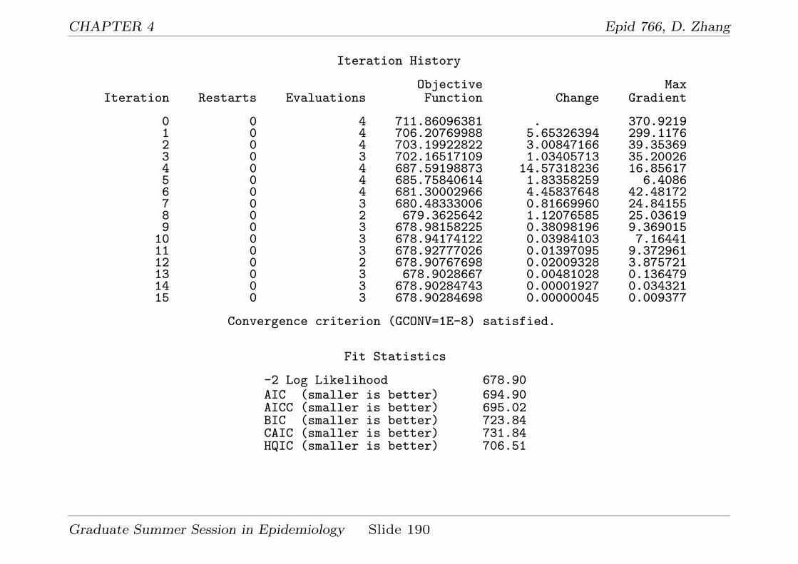
CHAPTER 4 Epid 766, D. Zhang
Iteration History
Objective MaxIteration Restarts Evaluations Function Change Gradient
0 0 4 711.86096381 . 370.92191 0 4 706.20769988 5.65326394 299.11762 0 4 703.19922822 3.00847166 39.353693 0 3 702.16517109 1.03405713 35.200264 0 4 687.59198873 14.57318236 16.856175 0 4 685.75840614 1.83358259 6.40866 0 4 681.30002966 4.45837648 42.481727 0 3 680.48333006 0.81669960 24.841558 0 2 679.3625642 1.12076585 25.036199 0 3 678.98158225 0.38098196 9.369015
10 0 3 678.94174122 0.03984103 7.1644111 0 3 678.92777026 0.01397095 9.37296112 0 2 678.90767698 0.02009328 3.87572113 0 3 678.9028667 0.00481028 0.13647914 0 3 678.90284743 0.00001927 0.03432115 0 3 678.90284698 0.00000045 0.009377
Convergence criterion (GCONV=1E-8) satisfied.
Fit Statistics
-2 Log Likelihood 678.90AIC (smaller is better) 694.90AICC (smaller is better) 695.02BIC (smaller is better) 723.84CAIC (smaller is better) 731.84HQIC (smaller is better) 706.51
Graduate Summer Session in Epidemiology Slide 190
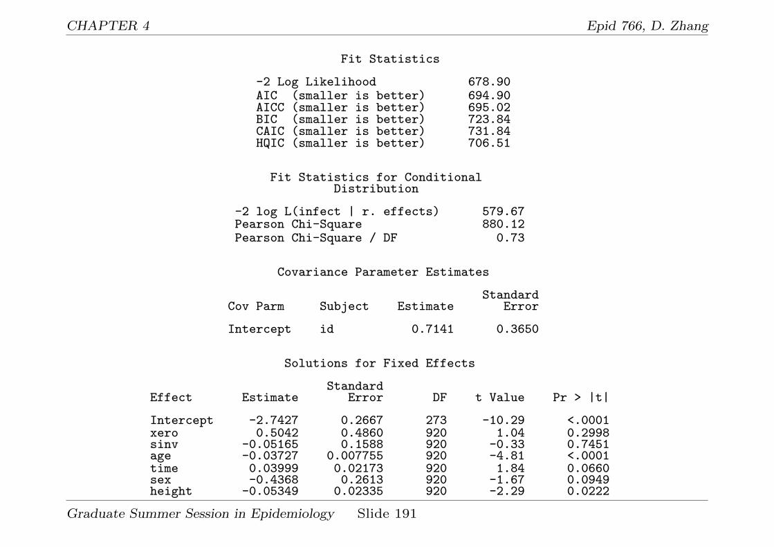
CHAPTER 4 Epid 766, D. Zhang
Fit Statistics
-2 Log Likelihood 678.90AIC (smaller is better) 694.90AICC (smaller is better) 695.02BIC (smaller is better) 723.84CAIC (smaller is better) 731.84HQIC (smaller is better) 706.51
Fit Statistics for ConditionalDistribution
-2 log L(infect | r. effects) 579.67Pearson Chi-Square 880.12Pearson Chi-Square / DF 0.73
Covariance Parameter Estimates
StandardCov Parm Subject Estimate Error
Intercept id 0.7141 0.3650
Solutions for Fixed Effects
StandardEffect Estimate Error DF t Value Pr > |t|
Intercept -2.7427 0.2667 273 -10.29 <.0001xero 0.5042 0.4860 920 1.04 0.2998sinv -0.05165 0.1588 920 -0.33 0.7451age -0.03727 0.007755 920 -4.81 <.0001time 0.03999 0.02173 920 1.84 0.0660sex -0.4368 0.2613 920 -1.67 0.0949height -0.05349 0.02335 920 -2.29 0.0222
Graduate Summer Session in Epidemiology Slide 191

CHAPTER 4 Epid 766, D. Zhang
• Remark 1 (subject-specific interpretation): Since
β1 = 0.5042, so if a child becomes Vitamin A deficiency from Vitamin
A sufficiency, his/her odds-ratio of getting respiratory infection will be
e0.5042 = 1.66, that is, about 66% increase in risk.
• Remark 2 (approximate population-average
interpretation): σ2b = 0.7141, so (1 + 0.346σ2
b )−1/2 = 0.9. So the
population-averaged effect of Vitamin A deficiency is
0.9× 0.5042 = 0.454. That is, given other covariates, the population
of children with Vitamin A deficiency will be 57% (odds-ratio
e0.454 = 1.57 ≈ relative risk if respiratory infection can be viewed as a
rare event) more likely to have respiratory infection than the
population of children without Vitamin A deficiency.
Graduate Summer Session in Epidemiology Slide 192

CHAPTER 4 Epid 766, D. Zhang
The population-average effect of sex is 0.9× (−0.4368) = −0.39
(odds-ratio = 0.65). So boys are less likely to have respiratory
infection than girls. Other effects can be obtained similarly.
• Remark 3: When the response yij is binary, we don’t have to worry
about over-dispersion for the conditional distribution of yij |bi.
Graduate Summer Session in Epidemiology Slide 193

CHAPTER 4 Epid 766, D. Zhang
4.4 Analyze epileptic count data using a GLMM
• Assume seizure counts
yij |bi ∼ Overdispersed− Poisson(µbij),
where
µbij = E(yij |bi) = tijλbij ,
λbij is the rate to have a seizure for subject i. Consider model
log(λbij) = β0 + β1I(j > 1) + β2trtiI(j > 1) + bi
log(µbij) = log(tij) + β0 + β1I(j > 1) + β2trtiI(j > 1) + bi,
where bi ∼ N(0, σ2b ) is a random intercept describing the
between-subject variation.
Graduate Summer Session in Epidemiology Slide 194

CHAPTER 4 Epid 766, D. Zhang
• Interpretation of β’s:
log(λb) for random subject i
Group Before RAND (j = 1) After RAND (j > 1)
Control (trt=0) β0 + bi β0 + β1 + bi
Treatment (trt=1) β0 + bi β0 + β1 + β2 + bi
β1: difference in log of rate of seizure counts comparing after
randomization and before randomization for a random subject in
control group (time + placebo effect).
β2: difference in log of rate of seizure counts for a treated subject
compared to if he/she received a placebo (treatment effect).
• For more details of the result, see SAS program seize mix.sas and its
output seize mix.lst
• Remark: Since here we used the Poisson GLMM with log link and a
random intercept, so the regression coefficients (except the intercept)
also have a population-averaged interpretation.
Graduate Summer Session in Epidemiology Slide 195

CHAPTER 4 Epid 766, D. Zhang
SAS program seize mix.sas
options ls=80 ps=1000 nodate;
/*------------------------------------------------------*//* *//* Proc Glimmix to fit random intercept model to the *//* epileptic seizure count data *//* *//*------------------------------------------------------*/
data seizure;infile "seize.dat";input id seize visit trt age;nobs=_n_;interval = 2;if visit=0 then interval=8;logtime = log(interval);assign = (visit>0);agn_trt = assign*trt;
run;
title "Random intercept model for seizure data with conditional overdispersion";proc glimmix data=seizure;
class id;model seize = assign agn_trt / dist=poisson link=log offset=logtime s;random int / subject=id type=vc;random _residual_; *for conditional overdispersion;
run;
Graduate Summer Session in Epidemiology Slide 196

CHAPTER 4 Epid 766, D. Zhang
SAS output seize mix.lst
Random intercept model for seizure data with conditional overdispersion 1
The GLIMMIX Procedure
Model Information
Data Set WORK.SEIZUREResponse Variable seizeResponse Distribution PoissonLink Function LogVariance Function DefaultOffset Variable logtimeVariance Matrix Blocked By idEstimation Technique Residual PLDegrees of Freedom Method Containment
Class Level Information
Class Levels Values
id 59 101 102 103 104 106 107 108 110 111 112 113114 ...
Number of Observations Read 295Number of Observations Used 295
Graduate Summer Session in Epidemiology Slide 197

CHAPTER 4 Epid 766, D. Zhang
Dimensions
G-side Cov. Parameters 1R-side Cov. Parameters 1Columns in X 3Columns in Z per Subject 1Subjects (Blocks in V) 59Max Obs per Subject 5
Optimization Information
Optimization Technique Dual Quasi-NewtonParameters in Optimization 1Lower Boundaries 1Upper Boundaries 0Fixed Effects ProfiledResidual Variance ProfiledStarting From Data
Iteration History
Objective MaxIteration Restarts Subiterations Function Change Gradient
0 0 4 609.19264304 0.49414053 0.0002051 0 5 671.59595217 0.14411653 3.061E-62 0 3 675.96769701 0.01612221 0.0000163 0 2 675.86073055 0.00032842 1.901E-84 0 1 675.85749753 0.00000336 3.111E-85 0 0 675.85746125 0.00000000 5.906E-6
Convergence criterion (PCONV=1.11022E-8) satisfied.
Graduate Summer Session in Epidemiology Slide 198

CHAPTER 4 Epid 766, D. Zhang
Fit Statistics
-2 Res Log Pseudo-Likelihood 675.86Generalized Chi-Square 822.08Gener. Chi-Square / DF 2.82
Covariance Parameter Estimates
StandardCov Parm Subject Estimate Error
Intercept id 0.5704 0.1169Residual (VC) 2.8154 0.2591
Solutions for Fixed Effects
StandardEffect Estimate Error DF t Value Pr > |t|
Intercept 1.0655 0.1079 58 9.88 <.0001assign 0.1122 0.07723 234 1.45 0.1477agn_trt -0.1063 0.1054 234 -1.01 0.3144
Graduate Summer Session in Epidemiology Slide 199

CHAPTER 4 Epid 766, D. Zhang
• Remark: There is considerable amount of over-dispersion for yij |bi.It is estimated that
var(yij |bi) = 2.82E(yij |bi).
• There is considerable between-patient variance in log-seizure rate.
That variation is estimated to be 0.57.
• The regression coefficient estimates (except the intercept) have
population-average interpretation, and they are almost the same as
those from the GEE model.
For example, β2 = −0.1063 with SE = 0.1054. Then if a subject
switches from control to treatment, the rate of having seizure will
decrease by 10% (since e−0.1063 = 0.9). The same rate deduction can
also be used to compare treatment and control groups (i.e., population
interpretation).
Graduate Summer Session in Epidemiology Slide 200

CHAPTER 4 Epid 766, D. Zhang
• If we would like to fit the data using the conditional quasi-likelihood
approach, we need to use Proc Nlmixed:proc nlmixed qpoints=15;parms beta0=-1.4 beta1=0.12 beta2=-0.12 theta=0.1 phi=1;eta = beta0 + beta1*assign + beta2*agn_trt + b;mu = interval*exp(eta);if seize=0 then
l = -(mu - seize)/phi - log(phi)/2;else
l = (seize*(log(mu) - log(seize)) - (mu - seize))/phi - log(phi)/2;model seize ~ general(l);random b ~ normal(0, theta) subject=id;
run;
Graduate Summer Session in Epidemiology Slide 201

CHAPTER 4 Epid 766, D. Zhang
The relevent output isParameter Estimates
StandardParameter Estimate Error DF t Value Pr > |t| Alpha Lower
beta0 1.0350 0.1100 58 9.41 <.0001 0.05 0.8148beta1 0.1123 0.07898 58 1.42 0.1603 0.05 -0.04577beta2 -0.1065 0.1077 58 -0.99 0.3269 0.05 -0.3222theta 0.5835 0.1204 58 4.85 <.0001 0.05 0.3426phi 2.9456 0.2684 58 10.98 <.0001 0.05 2.4084
Therefore, the between-patient variance is estimated to be 0.5835 and
the conditional over-dispersion parameter estimated to be φ = 2.9.
The inference on the treatment effect β2 is similar.
Graduate Summer Session in Epidemiology Slide 202

CHAPTER 4 Epid 766, D. Zhang
• If we would like to fit a generalized Poisson distribution for the
conditional distribution, we can use the following Proc Nlmixed
programproc nlmixed; * qpoints=15;
parms beta0=-1.4 beta1=0.12 beta2=-0.12 theta=0.1 xi=0.5;bound theta>0, xi>-1, xi<1;
eta = beta0 + beta1*assign + beta2*agn_trt + b;mu = interval*exp(eta);mu1 = (1-xi)*mu;mu2 = mu1 + xi*seize;
l = log(mu1) + (seize-1)*log(mu2) - mu2 - lgamma(seize+1);
model seize ~ general(l);random b ~ normal(0, theta) subject=id;
run;
Graduate Summer Session in Epidemiology Slide 203

CHAPTER 4 Epid 766, D. Zhang
The relevant output is
Parameter Estimates
StandardParameter Estimate Error DF t Value Pr > |t| Alpha Lower
beta0 1.0635 0.1061 58 10.02 <.0001 0.05 0.8510beta1 0.1256 0.08190 58 1.53 0.1307 0.05 -0.03837beta2 -0.1150 0.1110 58 -1.04 0.3043 0.05 -0.3372theta 0.5175 0.1076 58 4.81 <.0001 0.05 0.3020xi 0.4516 0.03048 58 14.81 <.0001 0.05 0.3906
The estimated between-patient variance is θ = 0.52 and the
conditional over-dispersion is 1/(1− ξ)2 = 1/(1− 0.4516)2 = 3.3. The
inference on the treatment effect β2 is again similar.
Graduate Summer Session in Epidemiology Slide 204
CHAPTER 5 Epid 766, D. Zhang
5 Summary: what we covered
1. Advantages of longitudinal studies over other classical studies.
2. Challenge in analyzing data from longitudinal studies: correlation,
within-subject and between-subject variation.
3. Linear mixed models for analyzing continuous longitudinal data:
random effects are explicitly used to model the between-subject
variation.
4. Generalized estimating equations (GEEs) for analyzing discrete
longitudinal data when the correlation is not of major interest.
Population-average interpretation.
5. Generalized linear mixed model for analyzing discrete longitudinal data
where random effects are used to model the correlation.
Subject-specific interpretation.
Graduate Summer Session in Epidemiology Slide 205