Embed Size (px)
Citation preview
Institute of the Environment and
Sustainability
CONTRIBUTING AUTHORS Anuradha Singh
Olivia JenkinsFlora Zepeda Torres
Samuel Hirsch Jeffrey Wolf
Alycia Cheng
AUTHORS | EDITORSMark Gold
Stephanie Pincetl Felicia Federico
EnvironmentalReport Card
FOR LOS ANGELES COUNTY
2015
Funded by the Goldhirsh Foundation

M E T R I C S 6
ECOSYSTEM
U C L A I N S T I T U T E O F T H E E N V I R O N M E N T A N D S U S TA I N A B I L I T Y 2 0 1 5 E N V I R O N M E N TA L R E P O RT C A R D F O R LO S A N G E L E S C O U N T Y42
E C O S Y S T E M H E A LT H
Los Angeles County has a Mediterranean-type climate, characterized by cool wet winters and warm dry summers. LA County is found in one of the most biodiverse parts of California, which includes most of the North American Mediterranean-climate zone and is itself a global biodiversity hotspot. This remarkable diversity of ecosystems provides extraordinary value to Los Angeles County residents through recreational and educational opportunities, as well as aesthetic enjoyment.
Overview
But these ecosystems are also under pressure from the 10 million residents (plus visitors), many of whom recreate in its protected open spaces on a regular basis. Extensive habitat loss and fragmentation, pollution, increased wildfire risk, and invasive species have taken their toll on the region’s ecosystems. And despite successful conservation efforts, numerous research projects and monitoring programs, and a regulatory
framework created to protect natural resources, assessing the state of the region’s ecosystems is extremely difficult as it requires the synthesis of disparate data sets for a very large region, including activities on both public and private lands. In addition, there are very few county-wide biological monitoring programs. For example, birds are the longest term, most widely monitored taxonomic group across the county. However, the bird counts
are in multiple large, non-standardized databases that were beyond our capability to analyze in time for this first report card. We recognize that the indicators presented here are woefully inadequate to characterize conditions and trends in ecosystem health, but we believe they represent the readily accessible, County-wide data sets available at this time.
U C L A I N S T I T U T E O F T H E E N V I R O N M E N T A N D S U S TA I N A B I L I T Y 2 0 1 5 E N V I R O N M E N TA L R E P O RT C A R D F O R LO S A N G E L E S C O U N T Y43
E C O S Y S T E M H E A LT H
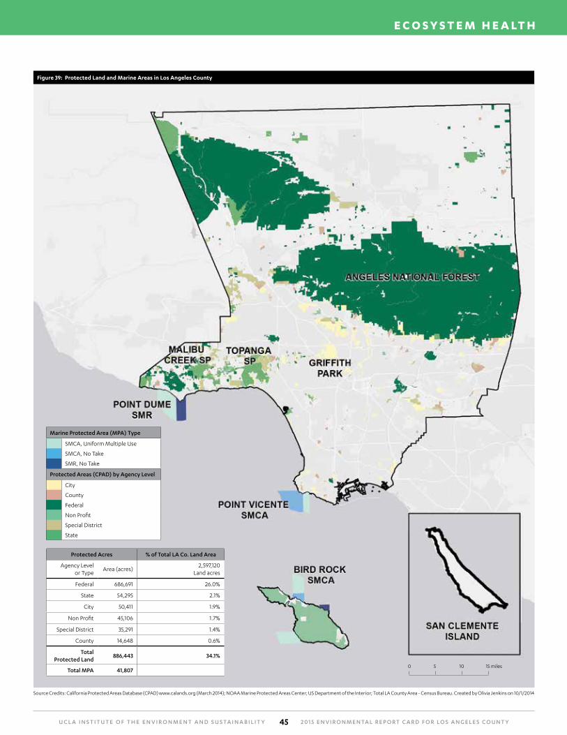
Protected AreasProtected areas in LA County provide long term conservation of habitats and species, as well as a range of other benefits. Within the county, these areas are major foci for outdoor recreation for over 10 million people. They also provide a wide range of services such as water quality improvements, carbon sequestration, and protection against extreme events including floods and storm surges.
land use protections for 50,000 acres of steep coastal watersheds and canyonlands. Also in 2014, major portions of the Angeles National Forest were included in the new San Gabriel National Monument, which will afford higher levels of protection for this richly biodiverse and geologically active mountain range, and one heavily used for recreation26.
Data
We used several measures of protected areas within LA County, all of which drew on data from the California Protected Areas Database27
Los Angeles has the great fortune of being situated at the base of vast National Forest lands. The mid-1970’s saw the addition of protected areas in the unique Santa Monica Mountain range and over the past 40 years, more lands have been added to the Santa Monica Mountains, and three Marine Protected Areas have also been created since 2012, located at Point Dume in Malibu, Point Vicente off Palos Verdes, and multiple locations off Santa Catalina Island.
In 2014, the Santa Monica Mountains Local Coastal Program (LCP) was adopted by the County Board of Supervisors and the California Coastal Commission, codifying
• Protected Lands and Marine Areas – these are public areas under management by Federal, State and local agencies and/or municipalities. These also include State Marine Conservation Areas (SMCA) and State Marine Reserves (SMR).
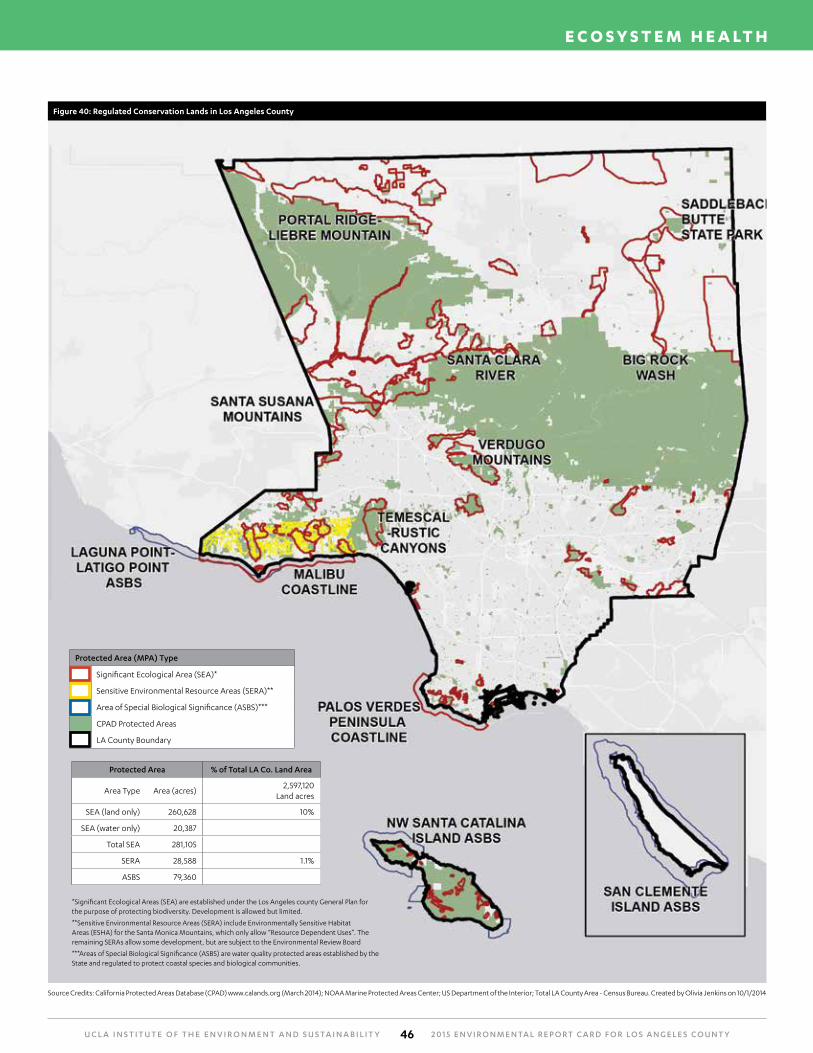
• Regulated Conservation Areas - these are public or private areas for which development or use is limited by regulation. Designations include Significant Ecological Areas (SEA), Sensitive Environmental Resource Areas (SERA) and Areas of Special Biological Significance (ASBS).
U C L A I N S T I T U T E O F T H E E N V I R O N M E N T A N D S U S TA I N A B I L I T Y 2 0 1 5 E N V I R O N M E N TA L R E P O RT C A R D F O R LO S A N G E L E S C O U N T Y44
E C O S Y S T E M H E A LT H
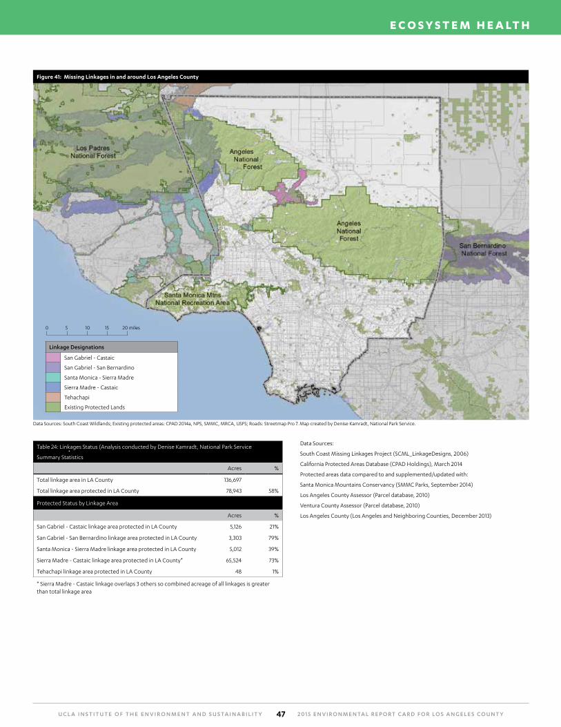
• Protected Lands Within Linkages – these public lands fall within designated landscape “linkages” that serve as corridors between large areas of core habitat. Such linkages are critical to maintaining healthy populations of many species, especially large carnivores, and provide opportunities for species’ range shifts to occur in response to climate change, particularly important within this heavily urbanized region. This analysis was conducted by the National Park Service, Santa Monica Mountains Recreation Area, and used data from the South Coast Missing Linkages Study conducted by South Coast Wildlands28.
Findings
• There are 886,443 acres of protected public lands in Los Angeles County, comprising 34% of the total County land area. There are 41,807 acres of marine protected areas. (Fig 39)
• Regulatory designations limiting development or use encompass a total of 10% of all County land area (Fig 40); land areas under these regulations that aren’t already in protected public ownership represent 8% of LA County land
• Protected areas are primarily restricted to high elevation, mountainous areas in the San Gabriels and (to a lesser extent) the Santa Monicas, with little protection in some areas such as southeast Los Angeles and the San Fernando Valley. In particular, nearly all of the protected areas are along the coast or in local mountains that are more difficult to develop. There are very few acres of protected area in the portions of the county with flat topography because this land has been utilized for urban development
• Out of 136,697 acres of wildlife linkage area within LA County, 58% (~79,000 acres) is currently protected public land. The areas with large missing wildlife linkages are: San Gabriel to Castaic in the Angeles National Forest, the Santa Monica Mountains to the Sierra Madre in Los Padres National Forest, and the
Sierra Madre to Castaic linkage between Los Padres and Angeles National Forests. (Fig 41)
The SMM LCP was over ten years in the making and is a major achievement for ecosystem protection in this area of the county. While the LA County General Plan update is making progress on a less-dispersed pattern of development, as reflected in lower rural densities and a town-center orientation, piecemeal sprawl development projects are still the status quo, for example in the “Town & Country” plan for the Antelope Valley, which at present includes low density development, more roads and highways, and little public transportation. LA County has no growth management system and lags behind Ventura County with its urban growth boundaries that protect habitat and farmland. Furthermore, unlike in neighboring counties (Riverside, Orange, San Diego), comprehensive habitat planning lags in LA, with only one Natural Communities Conservation Plan (in the Palos Verdes Peninsula) and with effective conservation efforts limited to those areas with specific and focused institutional structures in place, e.g., the Santa Monica Mountains. The designation of SEAs, particularly in view of the proposed expansions, constitutes a framework to protect what is left in the once-but-no-longer-remote lower elevations that historically have been lost to development and agriculture.
Data Limitations
• While the California Protected Areas Database fulfills a critical role of centralizing information on protected areas, the database relies on land management agencies and organizations to report land acquisitions, and therefore some public lands may not be currently included.
• We were unable to provide information on changes in vegetated area or vegetation type. However, work currently underway at UCLA (Gillespie lab) will soon be able to provide a historical assessment of vegetation and land use changes in Los Angeles County using remote sensing data. Possible
future evaluations also include land use changes within linkage areas and quantification of significant resources and vegetation types that are not currently protected.
U C L A I N S T I T U T E O F T H E E N V I R O N M E N T A N D S U S TA I N A B I L I T Y 2 0 1 5 E N V I R O N M E N TA L R E P O RT C A R D F O R LO S A N G E L E S C O U N T Y45
E C O S Y S T E M H E A LT H
Protected Acres % of Total LA Co. Land Area
Agency Level or Type
Area (acres)2,597,120
Land acres
Federal 686,691 26.0%
State 54,295 2.1%
City 50,411 1.9%
Non Profit 45,106 1.7%
Special District 35,291 1.4%
County 14,648 0.6%
Total Protected Land
886,443 34.1%
Total MPA 41,807
Marine Protected Area (MPA) Type
SMCA, Uniform Multiple Use
SMCA, No Take
SMR, No Take
Protected Areas (CPAD) by Agency Level
City
County
Federal
Non Profit
Special District
State
Source Credits: California Protected Areas Database (CPAD) www.calands.org (March 2014); NOAA Marine Protected Areas Center; US Department of the Interior; Total LA County Area - Census Bureau. Created by Olivia Jenkins on 10/1/2014
Figure 39: Protected Land and Marine Areas in Los Angeles County
0 5 10 15 miles
U C L A I N S T I T U T E O F T H E E N V I R O N M E N T A N D S U S TA I N A B I L I T Y 2 0 1 5 E N V I R O N M E N TA L R E P O RT C A R D F O R LO S A N G E L E S C O U N T Y46
E C O S Y S T E M H E A LT H
Protected Area % of Total LA Co. Land Area
Area Type Area (acres)2,597,120
Land acres
SEA (land only) 260,628 10%
SEA (water only) 20,387
Total SEA 281,105
SERA 28,588 1.1%
ASBS 79,360
Figure 40: Regulated Conservation Lands in Los Angeles County
*Significant Ecological Areas (SEA) are established under the Los Angeles county General Plan for the purpose of protecting biodiversity. Development is allowed but limited.
**Sensitive Environmental Resource Areas (SERA) include Environmentally Sensitive Habitat Areas (ESHA) for the Santa Monica Mountains, which only allow “Resource Dependent Uses”. The remaining SERAs allow some development, but are subject to the Environmental Review Board
***Areas of Special Biological Significance (ASBS) are water quality protected areas established by the State and regulated to protect coastal species and biological communities.
Protected Area (MPA) Type
Significant Ecological Area (SEA)*
Sensitive Environmental Resource Areas (SERA)**
Area of Special Biological Significance (ASBS)***
CPAD Protected Areas
LA County Boundary
Source Credits: California Protected Areas Database (CPAD) www.calands.org (March 2014); NOAA Marine Protected Areas Center; US Department of the Interior; Total LA County Area - Census Bureau. Created by Olivia Jenkins on 10/1/2014
U C L A I N S T I T U T E O F T H E E N V I R O N M E N T A N D S U S TA I N A B I L I T Y 2 0 1 5 E N V I R O N M E N TA L R E P O RT C A R D F O R LO S A N G E L E S C O U N T Y47
E C O S Y S T E M H E A LT H
Figure 41: Missing Linkages in and around Los Angeles County
Linkage Designations
San Gabriel - Castaic
San Gabriel - San Bernardino
Santa Monica - Sierra Madre
Sierra Madre - Castaic
Tehachapi
Existing Protected Lands
0 5 10 15 20 miles
Data Sources: South Coast Wildlands; Existing protected areas: CPAD 2014a, NPS, SMMC, MRCA, USFS; Roads: Streetmap Pro 7. Map created by Denise Kamradt, National Park Service.
Table 24: Linkages Status (Analysis conducted by Denise Kamradt, National Park Service
Summary Statistics
Acres %
Total linkage area in LA County 136,697
Total linkage area protected in LA County 78,943 58%
Protected Status by Linkage Area
Acres %
San Gabriel - Castaic linkage area protected in LA County 5,126 21%
San Gabriel - San Bernardino linkage area protected in LA County 3,303 79%
Santa Monica - Sierra Madre linkage area protected in LA County 5,012 39%
Sierra Madre - Castaic linkage area protected in LA County* 65,524 73%
Tehachapi linkage area protected in LA County 48 1%
* Sierra Madre - Castaic linkage overlaps 3 others so combined acreage of all linkages is greater than total linkage area
Data Sources:
South Coast Missing Linkages Project (SCML_LinkageDesigns, 2006)
California Protected Areas Database (CPAD Holdings), March 2014
Protected areas data compared to and supplemented/updated with:
Santa Monica Mountains Conservancy (SMMC Parks, September 2014)
Los Angeles County Assessor (Parcel database, 2010)
Ventura County Assessor (Parcel database, 2010)
Los Angeles County (Los Angeles and Neighboring Counties, December 2013)
U C L A I N S T I T U T E O F T H E E N V I R O N M E N T A N D S U S TA I N A B I L I T Y 2 0 1 5 E N V I R O N M E N TA L R E P O RT C A R D F O R LO S A N G E L E S C O U N T Y48
E C O S Y S T E M H E A LT H
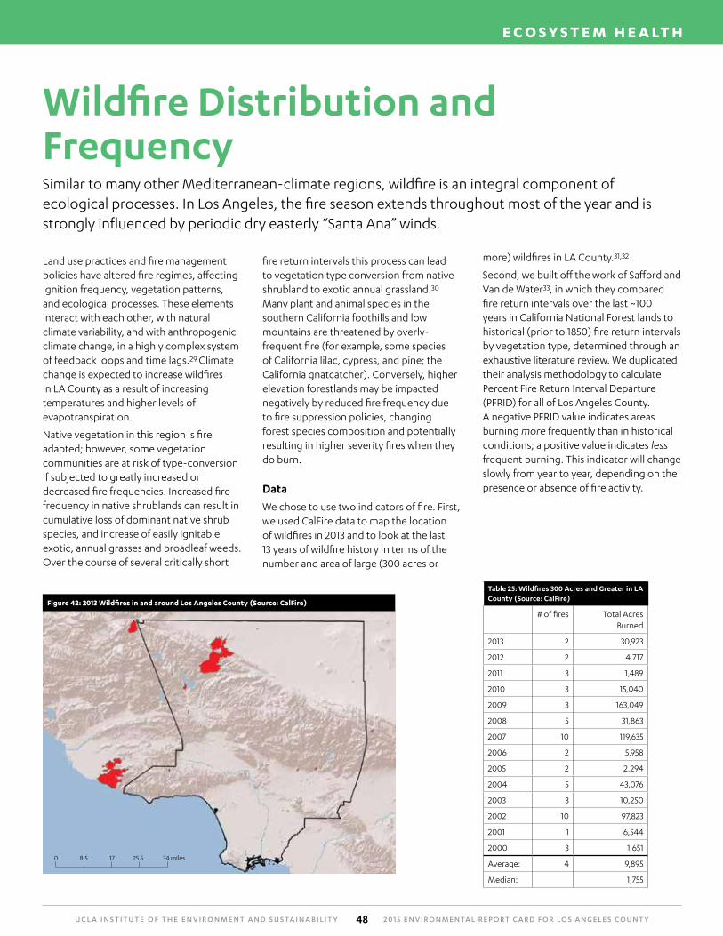
Wildfire Distribution and Frequency
Land use practices and fire management policies have altered fire regimes, affecting ignition frequency, vegetation patterns, and ecological processes. These elements interact with each other, with natural climate variability, and with anthropogenic climate change, in a highly complex system of feedback loops and time lags.29 Climate change is expected to increase wildfires in LA County as a result of increasing temperatures and higher levels of evapotranspiration.
Native vegetation in this region is fire adapted; however, some vegetation communities are at risk of type-conversion if subjected to greatly increased or decreased fire frequencies. Increased fire frequency in native shrublands can result in cumulative loss of dominant native shrub species, and increase of easily ignitable exotic, annual grasses and broadleaf weeds. Over the course of several critically short
fire return intervals this process can lead to vegetation type conversion from native shrubland to exotic annual grassland.30 Many plant and animal species in the southern California foothills and low mountains are threatened by overly-frequent fire (for example, some species of California lilac, cypress, and pine; the California gnatcatcher). Conversely, higher elevation forestlands may be impacted negatively by reduced fire frequency due to fire suppression policies, changing forest species composition and potentially resulting in higher severity fires when they do burn.
Data
We chose to use two indicators of fire. First, we used CalFire data to map the location of wildfires in 2013 and to look at the last 13 years of wildfire history in terms of the number and area of large (300 acres or
Similar to many other Mediterranean-climate regions, wildfire is an integral component of ecological processes. In Los Angeles, the fire season extends throughout most of the year and is strongly influenced by periodic dry easterly “Santa Ana” winds.
Figure 42: 2013 Wildfires in and around Los Angeles County (Source: CalFire)
0 8.5 17 25.5 34 miles
more) wildfires in LA County.31,32
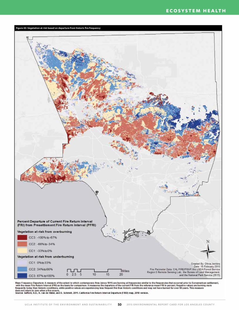
Second, we built off the work of Safford and Van de Water33, in which they compared fire return intervals over the last ~100 years in California National Forest lands to historical (prior to 1850) fire return intervals by vegetation type, determined through an exhaustive literature review. We duplicated their analysis methodology to calculate Percent Fire Return Interval Departure (PFRID) for all of Los Angeles County. A negative PFRID value indicates areas burning more frequently than in historical conditions; a positive value indicates less frequent burning. This indicator will change slowly from year to year, depending on the presence or absence of fire activity.
Table 25: Wildfires 300 Acres and Greater in LA County (Source: CalFire)
# of fires Total Acres Burned
2013 2 30,923
2012 2 4,717
2011 3 1,489
2010 3 15,040
2009 3 163,049
2008 5 31,863
2007 10 119,635
2006 2 5,958
2005 2 2,294
2004 5 43,076
2003 3 10,250
2002 10 97,823
2001 1 6,544
2000 3 1,651
Average: 4 9,895
Median: 1,755
U C L A I N S T I T U T E O F T H E E N V I R O N M E N T A N D S U S TA I N A B I L I T Y 2 0 1 5 E N V I R O N M E N TA L R E P O RT C A R D F O R LO S A N G E L E S C O U N T Y49
E C O S Y S T E M H E A LT H
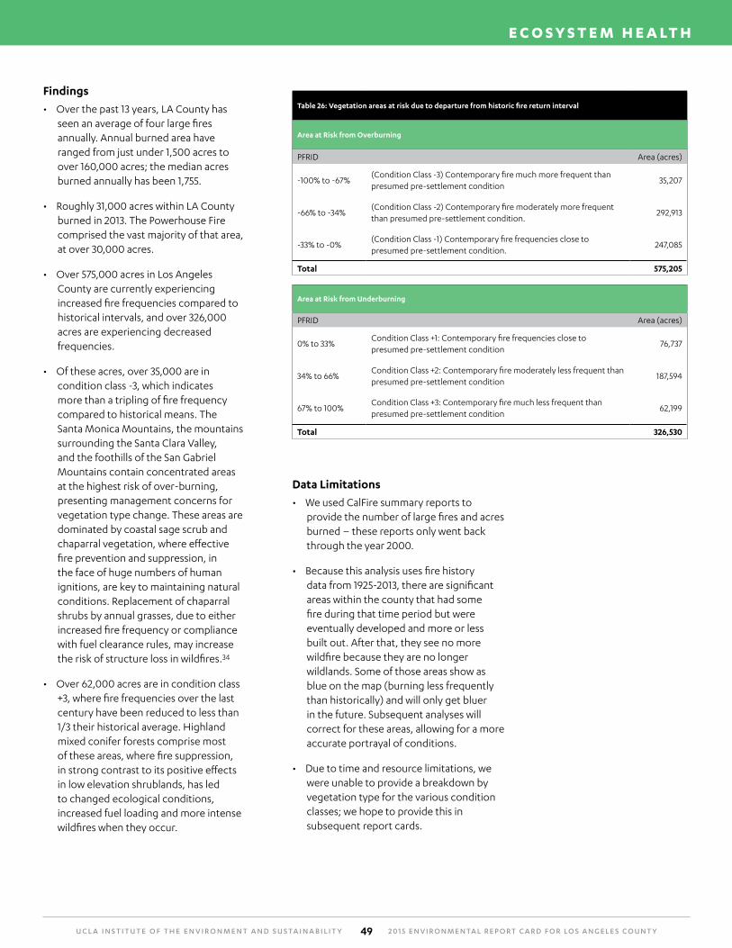
Findings
• Over the past 13 years, LA County has seen an average of four large fires annually. Annual burned area have ranged from just under 1,500 acres to over 160,000 acres; the median acres burned annually has been 1,755.
• Roughly 31,000 acres within LA County burned in 2013. The Powerhouse Fire comprised the vast majority of that area, at over 30,000 acres.
• Over 575,000 acres in Los Angeles County are currently experiencing increased fire frequencies compared to historical intervals, and over 326,000 acres are experiencing decreased frequencies.
• Of these acres, over 35,000 are in condition class -3, which indicates more than a tripling of fire frequency compared to historical means. The Santa Monica Mountains, the mountains surrounding the Santa Clara Valley, and the foothills of the San Gabriel Mountains contain concentrated areas at the highest risk of over-burning, presenting management concerns for vegetation type change. These areas are dominated by coastal sage scrub and chaparral vegetation, where effective fire prevention and suppression, in the face of huge numbers of human ignitions, are key to maintaining natural conditions. Replacement of chaparral shrubs by annual grasses, due to either increased fire frequency or compliance with fuel clearance rules, may increase the risk of structure loss in wildfires.34
• Over 62,000 acres are in condition class +3, where fire frequencies over the last century have been reduced to less than 1/3 their historical average. Highland mixed conifer forests comprise most of these areas, where fire suppression, in strong contrast to its positive effects in low elevation shrublands, has led to changed ecological conditions, increased fuel loading and more intense wildfires when they occur.
Table 26: Vegetation areas at risk due to departure from historic fire return interval
Area at Risk from Overburning
PFRID Area (acres)
-100% to -67%(Condition Class -3) Contemporary fire much more frequent than presumed pre-settlement condition
35,207
-66% to -34% (Condition Class -2) Contemporary fire moderately more frequent than presumed pre-settlement condition.
292,913
-33% to -0% (Condition Class -1) Contemporary fire frequencies close to presumed pre-settlement condition.
247,085
Total 575,205
Area at Risk from Underburning
PFRID Area (acres)
0% to 33% Condition Class +1: Contemporary fire frequencies close to presumed pre-settlement condition
76,737
34% to 66% Condition Class +2: Contemporary fire moderately less frequent than presumed pre-settlement condition
187,594
67% to 100% Condition Class +3: Contemporary fire much less frequent than presumed pre-settlement condition
62,199
Total 326,530
Data Limitations
• We used CalFire summary reports to provide the number of large fires and acres burned – these reports only went back through the year 2000.
• Because this analysis uses fire history data from 1925-2013, there are significant areas within the county that had some fire during that time period but were eventually developed and more or less built out. After that, they see no more wildfire because they are no longer wildlands. Some of those areas show as blue on the map (burning less frequently than historically) and will only get bluer in the future. Subsequent analyses will correct for these areas, allowing for a more accurate portrayal of conditions.
• Due to time and resource limitations, we were unable to provide a breakdown by vegetation type for the various condition classes; we hope to provide this in subsequent report cards.
U C L A I N S T I T U T E O F T H E E N V I R O N M E N T A N D S U S TA I N A B I L I T Y 2 0 1 5 E N V I R O N M E N TA L R E P O RT C A R D F O R LO S A N G E L E S C O U N T Y50
E C O S Y S T E M H E A LT H
Figure 43: Vegetation at risk based on departure from historic fire frequency
U C L A I N S T I T U T E O F T H E E N V I R O N M E N T A N D S U S TA I N A B I L I T Y 2 0 1 5 E N V I R O N M E N TA L R E P O RT C A R D F O R LO S A N G E L E S C O U N T Y51
E C O S Y S T E M H E A LT H
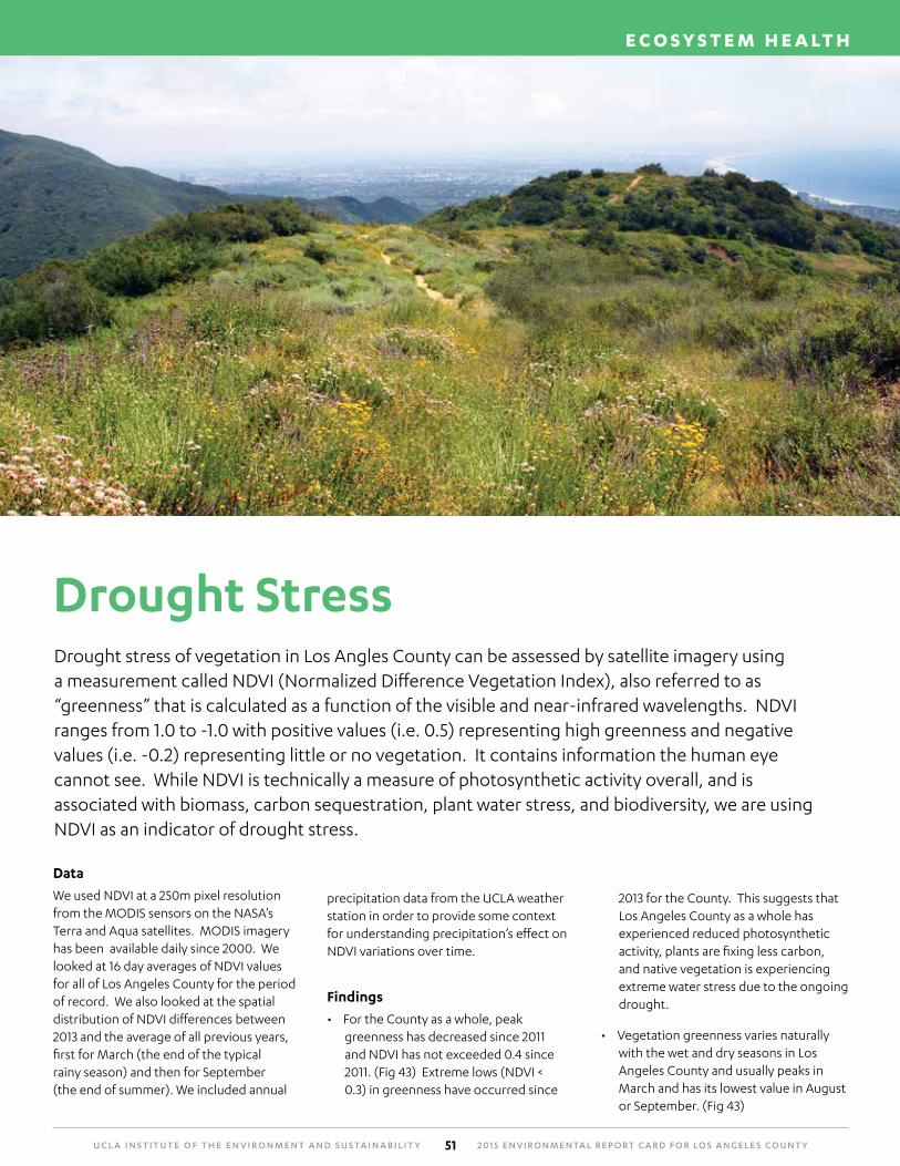
Drought stress of vegetation in Los Angles County can be assessed by satellite imagery using a measurement called NDVI (Normalized Difference Vegetation Index), also referred to as “greenness” that is calculated as a function of the visible and near-infrared wavelengths. NDVI ranges from 1.0 to -1.0 with positive values (i.e. 0.5) representing high greenness and negative values (i.e. -0.2) representing little or no vegetation. It contains information the human eye cannot see. While NDVI is technically a measure of photosynthetic activity overall, and is associated with biomass, carbon sequestration, plant water stress, and biodiversity, we are using NDVI as an indicator of drought stress.
Drought Stress
Data
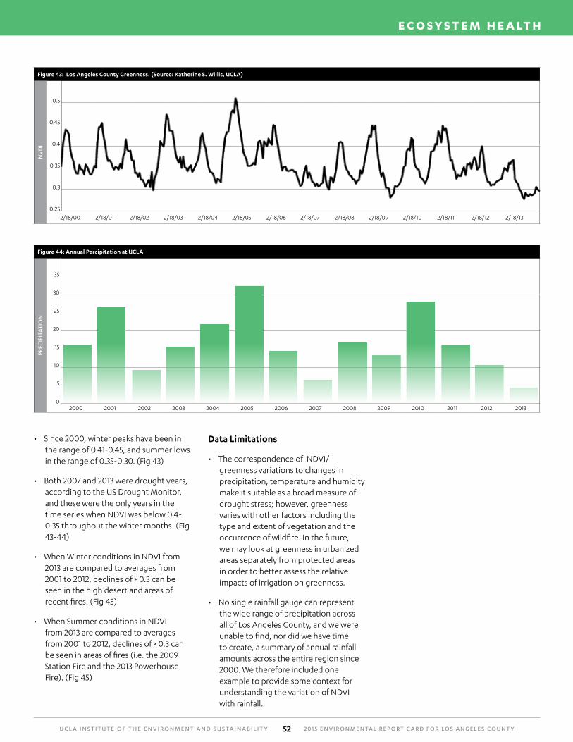
We used NDVI at a 250m pixel resolution from the MODIS sensors on the NASA’s Terra and Aqua satellites. MODIS imagery has been available daily since 2000. We looked at 16 day averages of NDVI values for all of Los Angeles County for the period of record. We also looked at the spatial distribution of NDVI differences between 2013 and the average of all previous years, first for March (the end of the typical rainy season) and then for September (the end of summer). We included annual
precipitation data from the UCLA weather station in order to provide some context for understanding precipitation’s effect on NDVI variations over time.
Findings
• For the County as a whole, peak greenness has decreased since 2011 and NDVI has not exceeded 0.4 since 2011. (Fig 43) Extreme lows (NDVI < 0.3) in greenness have occurred since
2013 for the County. This suggests that Los Angeles County as a whole has experienced reduced photosynthetic activity, plants are fixing less carbon, and native vegetation is experiencing extreme water stress due to the ongoing drought.
• Vegetation greenness varies naturally with the wet and dry seasons in Los Angeles County and usually peaks in March and has its lowest value in August or September. (Fig 43)
U C L A I N S T I T U T E O F T H E E N V I R O N M E N T A N D S U S TA I N A B I L I T Y 2 0 1 5 E N V I R O N M E N TA L R E P O RT C A R D F O R LO S A N G E L E S C O U N T Y52
E C O S Y S T E M H E A LT H
Figure 44: Annual Percipitation at UCLA
PREC
IPIT
ATI
ON
35
30
25
20
15
10
5
02000 2001 2002 2003 2004 2005 2006 2007 2008 2009 2010 2011 2012 2013
Figure 43: Los Angeles County Greenness. (Source: Katherine S. Willis, UCLA)
NV
DI
0.5
0.45
0.4
0.35
0.3
0.25
2/18/00 2/18/01 2/18/02 2/18/03 2/18/04 2/18/05 2/18/06 2/18/07 2/18/08 2/18/09 2/18/10 2/18/11 2/18/12 2/18/13
• Since 2000, winter peaks have been in the range of 0.41-0.45, and summer lows in the range of 0.35-0.30. (Fig 43)
• Both 2007 and 2013 were drought years, according to the US Drought Monitor, and these were the only years in the time series when NDVI was below 0.4-0.35 throughout the winter months. (Fig 43-44)
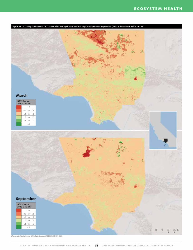
• When Winter conditions in NDVI from 2013 are compared to averages from 2001 to 2012, declines of > 0.3 can be seen in the high desert and areas of recent fires. (Fig 45)
• When Summer conditions in NDVI from 2013 are compared to averages from 2001 to 2012, declines of > 0.3 can be seen in areas of fires (i.e. the 2009 Station Fire and the 2013 Powerhouse Fire). (Fig 45)
Data Limitations
• The correspondence of NDVI/greenness variations to changes in precipitation, temperature and humidity make it suitable as a broad measure of drought stress; however, greenness varies with other factors including the type and extent of vegetation and the occurrence of wildfire. In the future, we may look at greenness in urbanized areas separately from protected areas in order to better assess the relative impacts of irrigation on greenness.
• No single rainfall gauge can represent the wide range of precipitation across all of Los Angeles County, and we were unable to find, nor did we have time to create, a summary of annual rainfall amounts across the entire region since 2000. We therefore included one example to provide some context for understanding the variation of NDVI with rainfall.
U C L A I N S T I T U T E O F T H E E N V I R O N M E N T A N D S U S TA I N A B I L I T Y 2 0 1 5 E N V I R O N M E N TA L R E P O RT C A R D F O R LO S A N G E L E S C O U N T Y53
E C O S Y S T E M H E A LT H
Figure 45. LA County Greenness in 2013 compared to average from 2000-2012. Top: March; Bottom: September. (Source: Katherine S. Willis, UCLA)
NDVI Change 2000-12 vs. 2013
< -.3
-.03 to -.15
-.15 to 0
0 to .15
.15 to .3
> .3
NDVI Change 2000-12 vs. 2013
< -.3
-.03 to -.15
-.15 to 0
0 to .15
.15 to .3
> .30 5 10 15 20 25 miles
March
September
Map created by Katherine Willis. Data Sources: MODIS MOD13Q1, ESRI
U C L A I N S T I T U T E O F T H E E N V I R O N M E N T A N D S U S TA I N A B I L I T Y 2 0 1 5 E N V I R O N M E N TA L R E P O RT C A R D F O R LO S A N G E L E S C O U N T Y54
E C O S Y S T E M H E A LT H
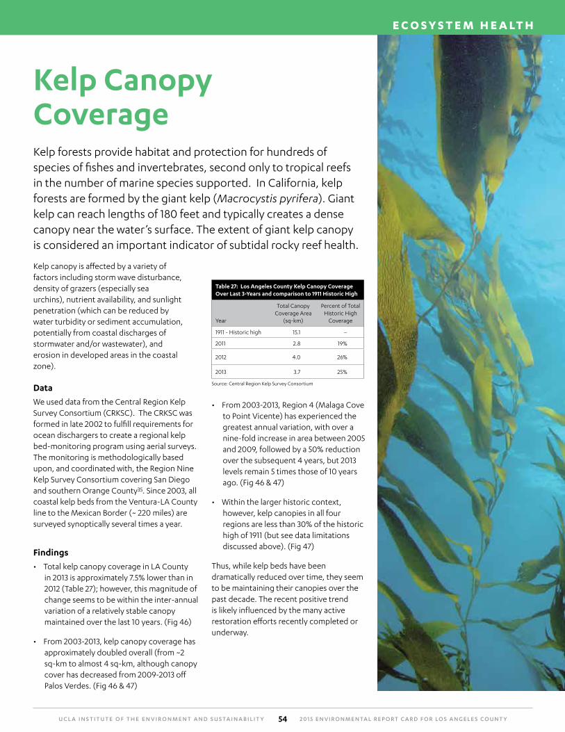
Kelp Canopy CoverageKelp forests provide habitat and protection for hundreds of species of fishes and invertebrates, second only to tropical reefs in the number of marine species supported. In California, kelp forests are formed by the giant kelp (Macrocystis pyrifera). Giant kelp can reach lengths of 180 feet and typically creates a dense canopy near the water’s surface. The extent of giant kelp canopy is considered an important indicator of subtidal rocky reef health.
Kelp canopy is affected by a variety of factors including storm wave disturbance, density of grazers (especially sea urchins), nutrient availability, and sunlight penetration (which can be reduced by water turbidity or sediment accumulation, potentially from coastal discharges of stormwater and/or wastewater), and erosion in developed areas in the coastal zone).
Data
We used data from the Central Region Kelp Survey Consortium (CRKSC). The CRKSC was formed in late 2002 to fulfill requirements for ocean dischargers to create a regional kelp bed-monitoring program using aerial surveys. The monitoring is methodologically based upon, and coordinated with, the Region Nine Kelp Survey Consortium covering San Diego and southern Orange County35. Since 2003, all coastal kelp beds from the Ventura-LA County line to the Mexican Border (~ 220 miles) are surveyed synoptically several times a year.
Findings
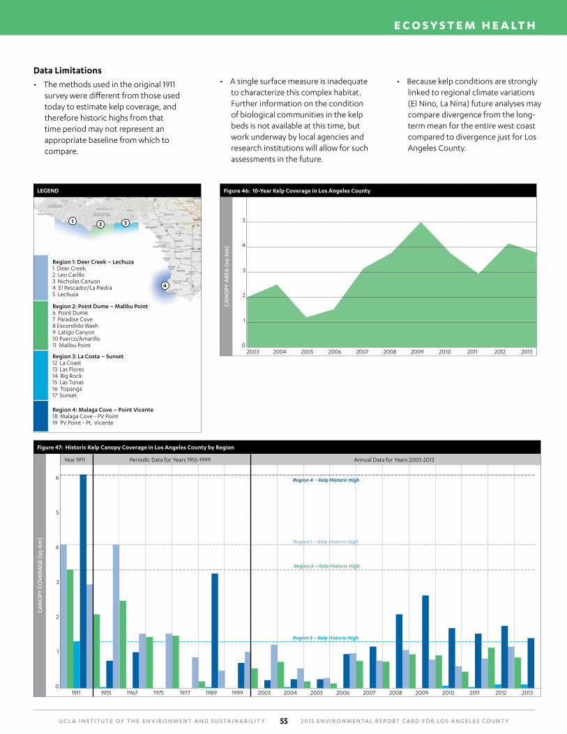
• Total kelp canopy coverage in LA County in 2013 is approximately 7.5% lower than in 2012 (Table 27); however, this magnitude of change seems to be within the inter-annual variation of a relatively stable canopy maintained over the last 10 years. (Fig 46)
• From 2003-2013, kelp canopy coverage has approximately doubled overall (from ~2 sq-km to almost 4 sq-km, although canopy cover has decreased from 2009-2013 off Palos Verdes. (Fig 46 & 47)
Table 27: Los Angeles County Kelp Canopy Coverage Over Last 3-Years and comparison to 1911 Historic High
Year
Total Canopy Coverage Area
(sq-km)
Percent of Total Historic High
Coverage
1911 - Historic high 15.1 –
2011 2.8 19%
2012 4.0 26%
2013 3.7 25%
Source: Central Region Kelp Survey Consortium
• From 2003-2013, Region 4 (Malaga Cove to Point Vicente) has experienced the greatest annual variation, with over a nine-fold increase in area between 2005 and 2009, followed by a 50% reduction over the subsequent 4 years, but 2013 levels remain 5 times those of 10 years ago. (Fig 46 & 47)
• Within the larger historic context, however, kelp canopies in all four regions are less than 30% of the historic high of 1911 (but see data limitations discussed above). (Fig 47)
Thus, while kelp beds have been dramatically reduced over time, they seem to be maintaining their canopies over the past decade. The recent positive trend is likely influenced by the many active restoration efforts recently completed or underway.
U C L A I N S T I T U T E O F T H E E N V I R O N M E N T A N D S U S TA I N A B I L I T Y 2 0 1 5 E N V I R O N M E N TA L R E P O RT C A R D F O R LO S A N G E L E S C O U N T Y55
E C O S Y S T E M H E A LT H
Region 1: Deer Creek – Lechuza1 Deer Creek2 Leo Carillo3 Nicholas Canyon4 El Pescador/La Piedra5 Lechuza
Region 2: Point Dume – Malibu Point6 Point Dume7 Paradise Cove8 Escondido Wash9 Latigo Canyon10 Puerco/Amarillo11 Malibu Point
Region 3: La Costa – Sunset12 La Coast13 Las Flores14 Big Rock15 Las Tunas16 Topanga17 Sunset
Region 4: Malaga Cove – Point Vicente18 Malaga Cove - PV Point19 PV Point - Pt. Vicente
LEGEND
1 2 3
4
Figure 46: 10-Year Kelp Coverage in Los Angeles County
CA
NO
PY A
REA
(sq
-km
)5
4
3
2
1
02003 2004 2005 2006 2007 2008 2009 2010 2011 2012 2013
Region 4 – Kelp Historic High
Region 1 – Kelp Historic High
Region 2 – Kelp Historic High
Region 3 – Kelp Historic High
Figure 47: Historic Kelp Canopy Coverage in Los Angeles County by Region
CA
NO
PY C
OV
ERA
GE
(sq-
km)
Year 1911 Periodic Data for Years 1955-1999 Annual Data for Years 2003-2013
6
5
4
3
2
1
01911 1955 1967 1975 1977 1989 1999 2003 2004 2005 2006 2007 2008 2009 2010 2011 2012 2013
Data Limitations
• The methods used in the original 1911 survey were different from those used today to estimate kelp coverage, and therefore historic highs from that time period may not represent an appropriate baseline from which to compare.
• A single surface measure is inadequate to characterize this complex habitat. Further information on the condition of biological communities in the kelp beds is not available at this time, but work underway by local agencies and research institutions will allow for such assessments in the future.
• Because kelp conditions are strongly linked to regional climate variations (El Nino, La Nina) future analyses may compare divergence from the long-term mean for the entire west coast compared to divergence just for Los Angeles County.
U C L A I N S T I T U T E O F T H E E N V I R O N M E N T A N D S U S TA I N A B I L I T Y 2 0 1 5 E N V I R O N M E N TA L R E P O RT C A R D F O R LO S A N G E L E S C O U N T Y56
E C O S Y S T E M H E A LT H
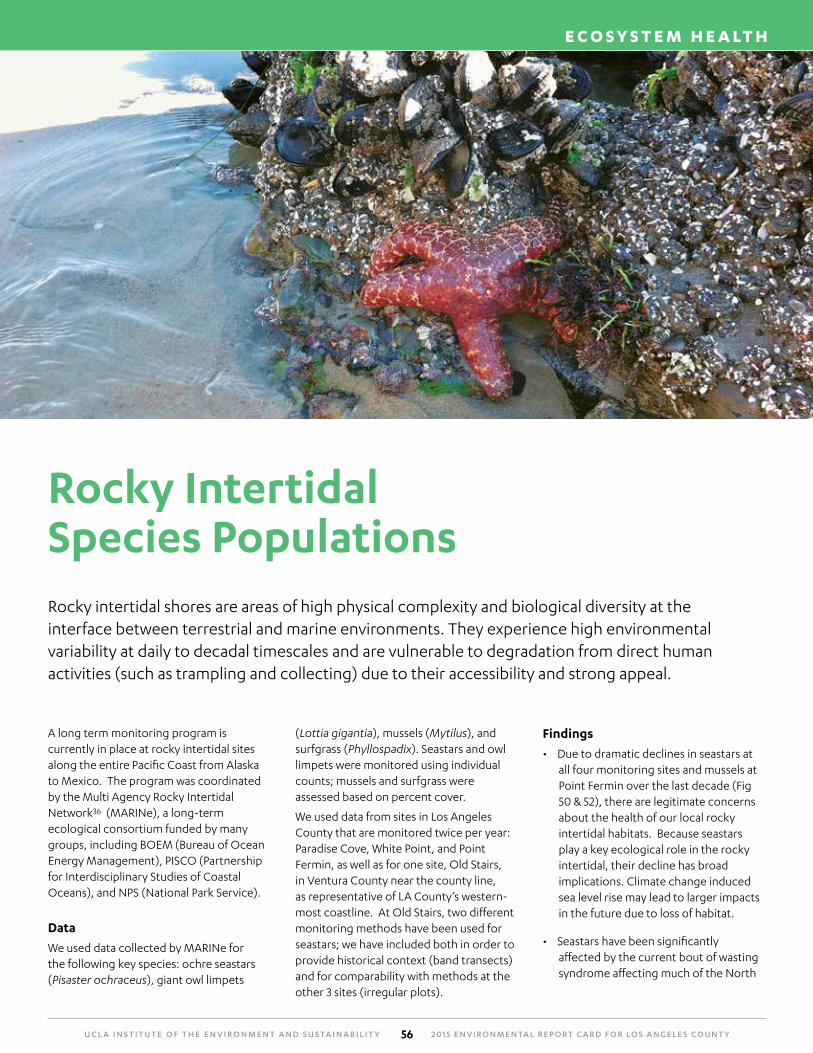
Rocky Intertidal Species PopulationsRocky intertidal shores are areas of high physical complexity and biological diversity at the interface between terrestrial and marine environments. They experience high environmental variability at daily to decadal timescales and are vulnerable to degradation from direct human activities (such as trampling and collecting) due to their accessibility and strong appeal.
A long term monitoring program is currently in place at rocky intertidal sites along the entire Pacific Coast from Alaska to Mexico. The program was coordinated by the Multi Agency Rocky Intertidal Network36 (MARINe), a long-term ecological consortium funded by many groups, including BOEM (Bureau of Ocean Energy Management), PISCO (Partnership for Interdisciplinary Studies of Coastal Oceans), and NPS (National Park Service).
Data
We used data collected by MARINe for the following key species: ochre seastars (Pisaster ochraceus), giant owl limpets
(Lottia gigantia), mussels (Mytilus), and surfgrass (Phyllospadix). Seastars and owl limpets were monitored using individual counts; mussels and surfgrass were assessed based on percent cover.
We used data from sites in Los Angeles County that are monitored twice per year: Paradise Cove, White Point, and Point Fermin, as well as for one site, Old Stairs, in Ventura County near the county line, as representative of LA County’s western-most coastline. At Old Stairs, two different monitoring methods have been used for seastars; we have included both in order to provide historical context (band transects) and for comparability with methods at the other 3 sites (irregular plots).
Findings
• Due to dramatic declines in seastars at all four monitoring sites and mussels at Point Fermin over the last decade (Fig 50 & 52), there are legitimate concerns about the health of our local rocky intertidal habitats. Because seastars play a key ecological role in the rocky intertidal, their decline has broad implications. Climate change induced sea level rise may lead to larger impacts in the future due to loss of habitat.
• Seastars have been significantly affected by the current bout of wasting syndrome affecting much of the North
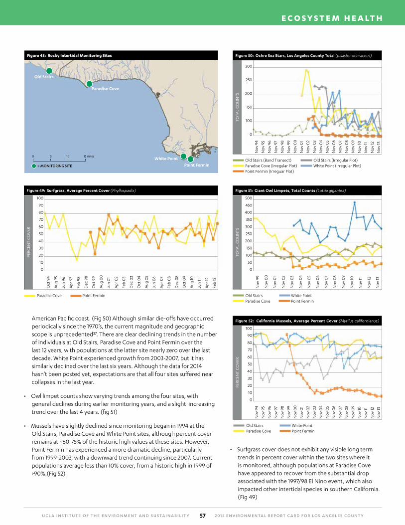
U C L A I N S T I T U T E O F T H E E N V I R O N M E N T A N D S U S TA I N A B I L I T Y 2 0 1 5 E N V I R O N M E N TA L R E P O RT C A R D F O R LO S A N G E L E S C O U N T Y57
E C O S Y S T E M H E A LT H
Figure 50: Ochre Sea Stars, Los Angeles County Total (pisaster ochraceus)
TOTA
L C
OU
NTS
300
250
200
150
100
0
No
v 94
No
v 95
No
v 96
No
v 97
No
v 98
No
v 99
No
v 0
0
No
v 0
1
No
v 0
2
No
v 0
3
No
v 0
4
No
v 0
5
No
v 0
6
No
v 0
7
No
v 0
8
No
v 0
9
No
v 10
No
v 11
No
v 12
No
v 13
Old Stairs (Band Transect) Old Stairs (Irregular Plot) Paradise Cove (Irregular Plot) White Point (Irregular Plot) Point Fermin (Irreguar Plot)
Figure 52: California Mussels, Average Percent Cover (Mytilus californianus)
PERC
ENT
CO
VER
100
90
80
70
60
50
40
30
20
10
0
No
v 94
No
v 95
No
v 96
No
v 97
No
v 98
No
v 99
No
v 0
0
No
v 0
1
No
v 0
2
No
v 0
3
No
v 0
4
No
v 0
5
No
v 0
6
No
v 0
7
No
v 0
8
No
v 0
9
No
v 10
No
v 11
No
v 12
No
v 13
Old Stairs White Point Paradise Cove Point Fermin
Figure 51: Giant Owl Limpets, Total Counts (Lottia gigantea)
TOTA
L C
OU
NTS
500
450
400
350
300
250
200
150
100
50
0
No
v 99
No
v 0
0
No
v 0
1
No
v 0
2
No
v 0
3
No
v 0
4
No
v 0
5
No
v 0
6
No
v 0
7
No
v 0
8
No
v 0
9
No
v 10
No
v 11
No
v 12
No
v 13
Old Stairs White Point Paradise Cove Point Fermin
Paradise Cove Point Fermin
Figure 49: Surfgrass, Average Percent Cover (Phyllospadix)
PERC
ENT
CO
VER
100
90
80
70
60
50
40
30
20
10
0
Oct
94
Aug
95
Jun
96
Apr
97
Feb
98
Dec
98
Oct
99
Aug
00
Jun
01
Apr
02
Feb
03
Dec
03
Oct
04
Aug
05
Jun
06
Apr
07
Feb
08
Dec
08
Oct
09
Aug
10
Jun
11
Apr
12
Feb
13
Figure 48: Rocky Intertidal Monitoring Sites
0 5 10 15 miles
Old Stairs
Paradise Cove
White Point
Point Fermin= MONITORING SITE
American Pacific coast. (Fig 50) Although similar die-offs have occurred periodically since the 1970’s, the current magnitude and geographic scope is unprecedented37. There are clear declining trends in the number of individuals at Old Stairs, Paradise Cove and Point Fermin over the last 12 years, with populations at the latter site nearly zero over the last decade. White Point experienced growth from 2003-2007, but it has similarly declined over the last six years. Although the data for 2014 hasn’t been posted yet, expectations are that all four sites suffered near collapses in the last year.
• Owl limpet counts show varying trends among the four sites, with general declines during earlier monitoring years, and a slight increasing trend over the last 4 years. (fig 51)
• Mussels have slightly declined since monitoring began in 1994 at the Old Stairs, Paradise Cove and White Point sites, although percent cover remains at ~60-75% of the historic high values at these sites. However, Point Fermin has experienced a more dramatic decline, particularly from 1999-2003, with a downward trend continuing since 2007. Current populations average less than 10% cover, from a historic high in 1999 of >90%.(Fig 52)
• Surfgrass cover does not exhibit any visible long term trends in percent cover within the two sites where it is monitored, although populations at Paradise Cove have appeared to recover from the substantial drop associated with the 1997/98 El Nino event, which also impacted other intertidal species in southern California. (Fig 49)
U C L A I N S T I T U T E O F T H E E N V I R O N M E N T A N D S U S TA I N A B I L I T Y 2 0 1 5 E N V I R O N M E N TA L R E P O RT C A R D F O R LO S A N G E L E S C O U N T Y58
E C O S Y S T E M H E A LT H
Data Limitations
• The monitoring sites were not randomly selected, but rather deliberately chosen in areas of high cover/number to ensure they represent “good” habitat for those species. This can result in initial apparent declines and therefore site conditions are generally evaluated based on long term trends after several years of monitoring have been completed.
• Only a few sites within LA County are being sampled, so we don’t have a good overview of the whole coastline.
• Focusing on a few species doesn’t capture what is happening to the community as a whole. It is an indicator of the health of the intertidal, but not a very comprehensive one.
• We have not included data for species that have already been removed from the intertidal, like abalone. This is important for the historical perspective of how humans have affected this community.
• These data do not examine some processes that could be important indicators of health, such as species recruitment or ability to recover from disturbance.
• These data do not include other attributes that are likely to be affected by ocean acidification, such as growth and recruitment.
U C L A I N S T I T U T E O F T H E E N V I R O N M E N T A N D S U S TA I N A B I L I T Y 2 0 1 5 E N V I R O N M E N TA L R E P O RT C A R D F O R LO S A N G E L E S C O U N T Y59
E C O S Y S T E M H E A LT H
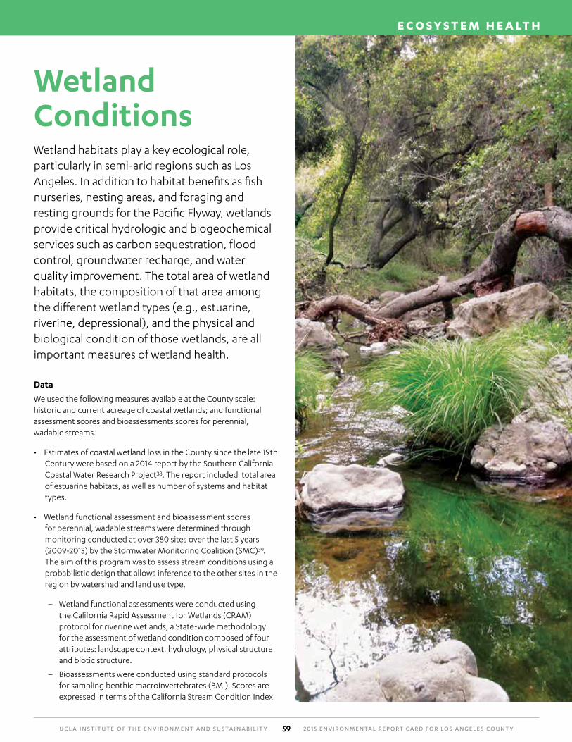
Wetland ConditionsWetland habitats play a key ecological role, particularly in semi-arid regions such as Los Angeles. In addition to habitat benefits as fish nurseries, nesting areas, and foraging and resting grounds for the Pacific Flyway, wetlands provide critical hydrologic and biogeochemical services such as carbon sequestration, flood control, groundwater recharge, and water quality improvement. The total area of wetland habitats, the composition of that area among the different wetland types (e.g., estuarine, riverine, depressional), and the physical and biological condition of those wetlands, are all important measures of wetland health.
Data
We used the following measures available at the County scale: historic and current acreage of coastal wetlands; and functional assessment scores and bioassessments scores for perennial, wadable streams.
• Estimates of coastal wetland loss in the County since the late 19th Century were based on a 2014 report by the Southern California Coastal Water Research Project38. The report included total area of estuarine habitats, as well as number of systems and habitat types.
• Wetland functional assessment and bioassessment scores for perennial, wadable streams were determined through monitoring conducted at over 380 sites over the last 5 years (2009-2013) by the Stormwater Monitoring Coalition (SMC)39. The aim of this program was to assess stream conditions using a probabilistic design that allows inference to the other sites in the region by watershed and land use type.
– Wetland functional assessments were conducted using the California Rapid Assessment for Wetlands (CRAM) protocol for riverine wetlands, a State-wide methodology for the assessment of wetland condition composed of four attributes: landscape context, hydrology, physical structure and biotic structure.
– Bioassessments were conducted using standard protocols for sampling benthic macroinvertebrates (BMI). Scores are expressed in terms of the California Stream Condition Index
U C L A I N S T I T U T E O F T H E E N V I R O N M E N T A N D S U S TA I N A B I L I T Y 2 0 1 5 E N V I R O N M E N TA L R E P O RT C A R D F O R LO S A N G E L E S C O U N T Y60
E C O S Y S T E M H E A LT H
(CSCI), which incorporates measures of BMI ecological structure, as well as a measure of taxonomic completeness in comparison to reference sites with similar characteristics (e.g., elevation, precipitation, etc).
• Maps and tables show results terms of four classifications, based on percentiles relative to a reference distribution (a normal estimate based on the mean and standard deviation of reference sites), calculated and provided by SCCWRP.
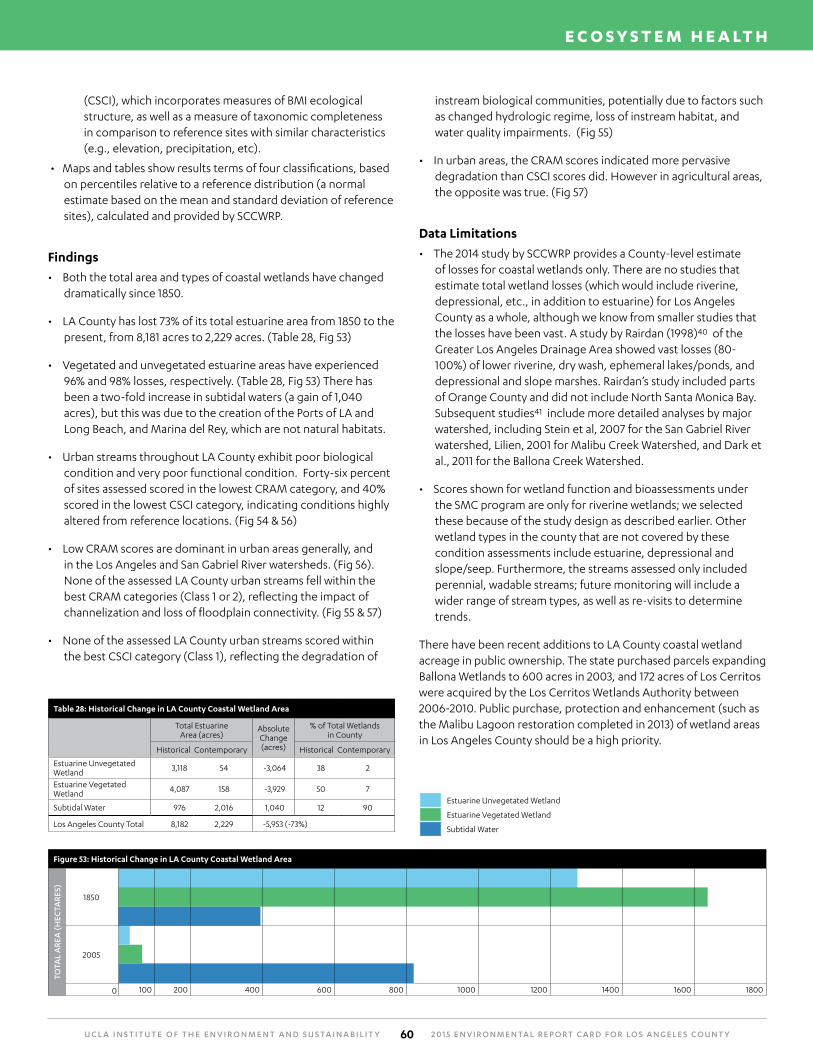
Findings
• Both the total area and types of coastal wetlands have changed dramatically since 1850.
• LA County has lost 73% of its total estuarine area from 1850 to the present, from 8,181 acres to 2,229 acres. (Table 28, Fig 53)
• Vegetated and unvegetated estuarine areas have experienced 96% and 98% losses, respectively. (Table 28, Fig 53) There has been a two-fold increase in subtidal waters (a gain of 1,040 acres), but this was due to the creation of the Ports of LA and Long Beach, and Marina del Rey, which are not natural habitats.
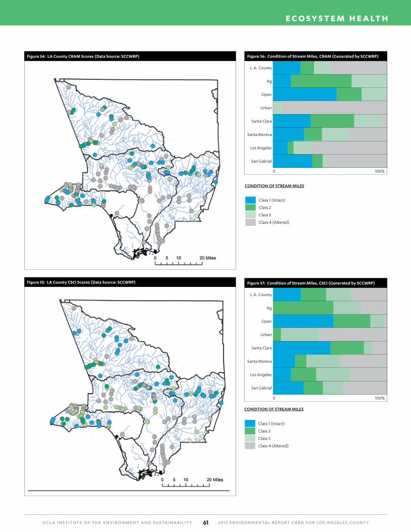
• Urban streams throughout LA County exhibit poor biological condition and very poor functional condition. Forty-six percent of sites assessed scored in the lowest CRAM category, and 40% scored in the lowest CSCI category, indicating conditions highly altered from reference locations. (Fig 54 & 56)
• Low CRAM scores are dominant in urban areas generally, and in the Los Angeles and San Gabriel River watersheds. (Fig 56). None of the assessed LA County urban streams fell within the best CRAM categories (Class 1 or 2), reflecting the impact of channelization and loss of floodplain connectivity. (Fig 55 & 57)
• None of the assessed LA County urban streams scored within the best CSCI category (Class 1), reflecting the degradation of
Estuarine Unvegetated Wetland
Estuarine Vegetated Wetland
Subtidal Water
Table 28: Historical Change in LA County Coastal Wetland Area
Total EstuarineArea (acres)
AbsoluteChange (acres)
% of Total Wetlands in County
Historical Contemporary Historical Contemporary
Estuarine Unvegetated Wetland 3,118 54 -3,064 38 2
Estuarine Vegetated Wetland 4,087 158 -3,929 50 7
Subtidal Water 976 2,016 1,040 12 90
Los Angeles County Total 8,182 2,229 -5,953 (-73%)
Figure 53: Historical Change in LA County Coastal Wetland Area
TOTA
L A
REA
(H
ECTA
RES)
1850
2005
0 100 200 400 600 800 1000 1200 1400 1600 1800
instream biological communities, potentially due to factors such as changed hydrologic regime, loss of instream habitat, and water quality impairments. (Fig 55)
• In urban areas, the CRAM scores indicated more pervasive degradation than CSCI scores did. However in agricultural areas, the opposite was true. (Fig 57)
Data Limitations
• The 2014 study by SCCWRP provides a County-level estimate of losses for coastal wetlands only. There are no studies that estimate total wetland losses (which would include riverine, depressional, etc., in addition to estuarine) for Los Angeles County as a whole, although we know from smaller studies that the losses have been vast. A study by Rairdan (1998)40 of the Greater Los Angeles Drainage Area showed vast losses (80-100%) of lower riverine, dry wash, ephemeral lakes/ponds, and depressional and slope marshes. Rairdan’s study included parts of Orange County and did not include North Santa Monica Bay. Subsequent studies41 include more detailed analyses by major watershed, including Stein et al, 2007 for the San Gabriel River watershed, Lilien, 2001 for Malibu Creek Watershed, and Dark et al., 2011 for the Ballona Creek Watershed.
• Scores shown for wetland function and bioassessments under the SMC program are only for riverine wetlands; we selected these because of the study design as described earlier. Other wetland types in the county that are not covered by these condition assessments include estuarine, depressional and slope/seep. Furthermore, the streams assessed only included perennial, wadable streams; future monitoring will include a wider range of stream types, as well as re-visits to determine trends.
There have been recent additions to LA County coastal wetland acreage in public ownership. The state purchased parcels expanding Ballona Wetlands to 600 acres in 2003, and 172 acres of Los Cerritos were acquired by the Los Cerritos Wetlands Authority between 2006-2010. Public purchase, protection and enhancement (such as the Malibu Lagoon restoration completed in 2013) of wetland areas in Los Angeles County should be a high priority.
U C L A I N S T I T U T E O F T H E E N V I R O N M E N T A N D S U S TA I N A B I L I T Y 2 0 1 5 E N V I R O N M E N TA L R E P O RT C A R D F O R LO S A N G E L E S C O U N T Y61
E C O S Y S T E M H E A LT H
Figure 57: Condition of Stream Miles, CSCI (Generated by SCCWRP)
L.A. County
Ag
Open
Urban
Santa Clara
Santa Monica
Los Angeles
San Gabriel
0 100%
CONDITION OF STREAM MILES
Class 1 (Intact)
Class 2
Class 3
Class 4 (Altered)
Figure 56: Condition of Stream Miles, CRAM (Generated by SCCWRP)
L.A. County
Ag
Open
Urban
Santa Clara
Santa Monica
Los Angeles
San Gabriel
0 100%
Figure 54: LA County CRAM Scores (Data Source: SCCWRP)
Figure 55: LA County CSCI Scores (Data Source: SCCWRP)
CONDITION OF STREAM MILES
Class 1 (Intact)
Class 2
Class 3
Class 4 (Altered)
U C L A I N S T I T U T E O F T H E E N V I R O N M E N T A N D S U S TA I N A B I L I T Y 2 0 1 5 E N V I R O N M E N TA L R E P O RT C A R D F O R LO S A N G E L E S C O U N T Y62
E C O S Y S T E M H E A LT H
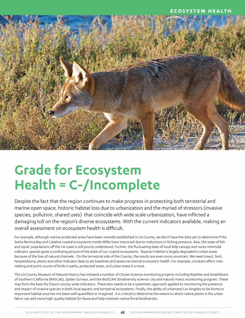
Grade for Ecosystem Health = C-/IncompleteDespite the fact that the region continues to make progress in protecting both terrestrial and marine open space, historic habitat loss due to urbanization and the myriad of stressors (invasive species, pollution, shared uses) that coincide with wide scale urbanization, have inflicted a damaging toll on the region’s diverse ecosystems. With the current indicators available, making an overall assessment on ecosystem health is difficult.
For example, although marine protected areas have been recently established in LA County, we don’t have the data yet to determine if the Santa Monica Bay and Catalina coastal ecosystems inside MPAs have improved due to reductions in fishing pressure. Also, the state of fish and squid populations off the LA coast is still poorly understood. Further, the fluctuating state of local kelp canopy and rocky intertidal indicator species gives a confusing picture of the state of our coastal ecosystems. Riparian habitat is largely degraded in urban areas because of the loss of natural channels. On the terrestrial side of the County, the results are even more uncertain. We need insect, bird, herpetofauna, plants and other indicator data to set baselines and assess terrestrial ecosystem health. For example, constant effort mist-netting and point counts of birds in parks, protected areas, and urban areas is a must.
The LA County Museum of Natural History has initiated a number of Citizen Science monitoring projects including Reptiles and Amphibians of Southern California (RASCals), Spider Surveys, and the BioSCAN (biodiversity science: city and nature) insect monitoring program. These may form the basis for future county-wide indicators. There also needs to be a systematic approach applied to monitoring the presence and impact of invasive species in both local aquatic and terrestrial ecosystems. Finally, the ability of urbanized Los Angeles to be home to important habitat area has not been well quantified or imagined. It is critical to determine the extent to which native plants in the urban fabric can add more high-quality habitat for fauna and help maintain native floral biodiversity.
UCLA Institute of the Environment and Sustainability La Kretz Hall, Suite 300
Box 951496 Los Angeles, CA 90095-1496
Tel: (310) 825-5008 Fax: (310) 825-9663
[email protected] www.environment.ucla.edu