Environmental Regulation and Firm Exports: Evidence from ...crm.sem.tsinghua.edu.cn/UploadFiles/File/201711/20171109115442593.… · In this paper, we take advantage of China’s

1

Environmental Regulation and Firm Exports: Evidence from the

Eleventh Five-Year Plan in China

October 2017

Abstract

Combining time variations, cross-province variations in policy intensity,

and variations in pollution intensity across industries, we estimate the impact of

environmental regulation on firm exports. We find that in more

pollution-intensive industries, stricter environmental regulation reduces both the

probability that a firm will export and the volume of exports. Heterogeneous

tests show that the impact is smaller for SOE firms and for firms located in the

central and western part of China. We also find that the reduced probability that

a firm will export is driven by a decline in non-exporters entering the export

market.

Key words: environmental regulation; exports; China

JEL codes: F10; F18; Q53; Q56

2

1. Introduction

In response to the growing deterioration of the environment, many

governments across the world are tightening their pollution regulations in the

hope that firms will adopt more environmentally friendly technology. However,

variations in the stringency of these regulations across countries suggest that the

cost of production for polluting industries in countries with stricter

environmental regulations is relatively higher, thereby deterring exports and the

inflow of foreign capital in these industries. Taylor (2004) calls this a “pollution

haven effect” (PHE).

Studying the PHE has important policy implications. First, the

effectiveness of global efforts to reduce greenhouse gas emissions may be

undermined by the concentration of polluting industries in countries with lax

environmental regulations. Second, the concentration of polluting industries in

countries with lax regulations imposes a substantial health cost and therefore

affects the welfare level in these countries.1 Third, the existence of the PHE has

important implications for international trade negotiations when there is debate

over whether to expand trade agreements to include cooperation with domestic

policies (Ederington and Minier, 2003).

Despite the importance of the PHE, there is no consensus across current

studies. Some studies find small and unimportant effects,2 while others claim

1 See Greenstone and Hanna (2011), Hanna and Oliva (2011), Chen et al. (2013), and He, Fan, and Zhou (2016). 2 These studies include but are not limited to Tobey (1990), Grossman and Krueger (1993), Jaffe et al. (1995), Levinson (1996), Antweiler et al. (2001), and Javorcik and Wei (2004).

3

more significant effects.3 Dean et al. (2009) attribute the insignificant evidence

for the PHE to the failure to account for the endogenous environmental

regulations. Indeed, a meta-analysis conducted by Jeppesen et al. (2002) points

out that much of the variation in findings on the effects of environmental

regulations can be attributed to differences in methodology.4

In this paper, we take advantage of China’s eleventh Five-Year Plan to

investigate this question. The plan establishes a pollution reduction target for the

entire country with different provinces sharing different burdens. To achieve

pollution reduction targets, provinces with higher targets exert greater effort.

Accordingly, this provides both before-and-after variation and cross-province

variation for identification. However, a simple difference-in-differences strategy

cannot exclude provincial-level time-varying variables that may bias the

estimates. We therefore apply a difference-in-difference-in-differences (DDD)

strategy to identify the impact. In other words, we compare the before-and-after

change of firms in industries with different pollution intensities in different

provinces. To further address the potential endogenous provincial pollution

reduction targets, we use the ventilation coefficient, which is the product of

wind speed and mixing height, as an instrumental variable (IV) for provincial

Copeland and Taylor (2004) provide a detailed literature review. 3 These studies include but are not limited to Henderson (1996), Becker and Henderson (2000), List and Co (2000), Keller and Levinson (2002), List, et al. (2003), Ederington and Minier (2003), Levinson and Taylor (2008), Kellenberg (2009), Broner, Bustos, and Carvalho (2013), Hering and Poncet (2014), and Cai et al. (2016). Copeland and Taylor (2004) and Erdogan (2014) provide literature reviews. 4 In our paper, we find significant evidence for the PHE. This could be because we use a policy change in China (together with instrumental variable strategy) for identification, which avoids potential bias due to the endogeneity problem.

4

pollution reduction targets. Compared with the period before the eleventh

Five-Year Plan, we find that firms in more pollution-intensive industries located

in provinces with higher pollution reduction targets are less likely to export, and

if they do export, to export less.

Several robustness checks justify this finding. We first show that the

pre-existing time trends of firm exports are similar across firms in different

industries and different provinces. We then show that concurrent events, such as

value-added tax reform, the 2008 Beijing Olympic Games, and the 2008-2009

financial crisis, do not affect our estimates. We also find that our results are

robust for the different samples and different measurements of policy intensity.

In addition, we find smaller effects for SOE firms and firms located in the

central and western part of China. Furthermore, we find that the decline in the

probability of firms exporting is primarily driven by a reduced probability of

non-exporters entering the export market.

Beyond the aforementioned policy implications, this paper contributes to

the literature in other ways. First, compared with studies using data from

developed countries such as the U.S. (Hanna, 2011; Millimet and Roy, 2016)

and South Korea (Chung, 2014), investigating the PHE in the context of a

developing country (i.e., China) is important because such countries have

always been the focus of debate about pollution havens (Blonigen and Wang,

2005). Focusing on China is of particular importance in investigating the PHE.

On the one hand, unlike developed countries such as the U.S. where the

5

economy is in a stable stage, China has experienced fast economic growth in the

past decades. China’s economy growth has been accompanied by severe

environmental deterioration, which is typical during rapid economic growth. On

the other hand, since China entered the WTO in 2001, Chinese exports have

increased dramatically. In 2016, Chinese exports were ranked the highest in the

world and accounted for about 20% of GDP.5 Investigating the PHE can shed

light on the tradeoff between a stringent environmental policy and exports,

which ultimately affects China’s long-term economic growth. Last but not least,

studying the PHE in China is advantageous because the policy change in China

provides a good opportunity to circumvent the endogeneity problem, which is

the greatest challenge for empirical studies.

Second, there are other studies investigating the effects of stricter

environmental regulations in China. However, some of these studies focus on

foreign direct investment (such as Dean et al., 2009, and Cai et al., 2016).

Compared with other papers (such as Hering and Poncet, 2014) that investigate

the effects of stricter environmental regulations on exports in China, we go a

step further to investigate whether stricter regulations affect exports by inducing

incumbents to cease exporting or by preventing non-exporters from entering the

export market.

Third, our paper can also be linked with the rapidly growing body of

5 The 2016 export data are extracted from the United Nations Comtrade Database (https://comtrade.un.org/). The percentage of exports in GDP is taken from the World Bank database (https://data.worldbank.org/indicator/NE.EXP.GNFS.ZS).

6

literature on international trade in which domestic institutions or policies are

treated as sources of comparative advantage. For example, using Chinese data,

Gan, Hernandez, and Ma (2016) find a significant negative relationship between

changes to the minimum wage and firm exports.6 This paper extends this

literature by providing evidence that domestic environmental policies are also

an important source of comparative advantage.

The remainder of this paper is structured as follows. Section 2 provides

background information. Section 3 describes the data. Section 4 describes the

empirical strategy. Section 5 shows the main results and includes several

robustness checks. Section 6 investigates the channels, and Section 7 concludes

the paper.

2. Background

China’s five-year plans are a series of countrywide social and economic

development initiatives containing detailed guidelines for economic and social

development. The first Five-Year Plan ran from 1953 to 1957 and the eleventh

Five-Year Plan (under study) ran from 2006 to 2010. Although economic

growth was originally the central task of the five-year plans, the tenth Five-Year

Plan (2001–2005) was the first to include an environmental policy by setting a

10% SO� reduction target. However, the tenth Five-Year Plan did not set

pollution reduction target for each province and it lacked a clearly defined

6 For a more detailed survey of the literature, readers are referred to Nunn and Trefler (2014).

7

evaluation scheme, implementation of the target was completely ineffective.

Total SO� emission increased by roughly 28% from 20 million tons in 2000 to

25.5 million tons in 2005.7

The eleventh Five-Year Plan also set 10% as its SO� reduction target. In

establishing the SO� reduction goals, two factors were the most important:

long-term goals and designated achievement years. To determine its long-term

SO� emission goals, the Chinese government relied on environmental carrying

capacity, i.e., the maximum emissions allowable without degrading

environmental quality below a minimum level (Yang et al., 1998, 1999). Based

on sophisticated scientific calculations, the long-term goal was an ambient SO�

concentration of 0.060 mg/m� within grid boxes of 1° ∗ 1° (i.e., about 111 km

∗111 km), requiring that SO� emissions be reduced to 18 million tons by 2020.

Thus, the 10% SO� reduction goal was proposed in the eleventh Five-Year

Plan (Xu, 2011).

After the national goal was established, the provinces negotiated with

the central government for their share of the burden (Xu, 2011). The China State

Council issued a document named “Reply to Pollution Control Plan During the

Eleventh Five-Year Plan” in 2006, which handed down national goal to

pollution reduction targets in provincial level. 8 Formal contracts for the

provincial pollution reduction targets were signed by the provincial vice

7 The SO� emission data are from the China Statistical Yearbook (2001, 2006). 8 This document lists total SO� emission for each province in 2005, SO� emission target

for each province in 2010, SO� emission target for electricity sector in each province in 2010, and the reduction percentage target for each province.

8

presidents (State Environment Protection Administration, 2006). As shown in

Figure 1, the mean of the reduction targets is 9.6% and the standard deviation is

6.8%. However, the negotiation process is not publicly available. Using other

publicly available data, Xu (2011) shows that the 2005 provincial SO�

emissions and non-power sector SO� emission density are significantly

correlated with the provinces’ shared target. We therefore deduce that initial

environmental quality was the most important factor in determining pollution

reduction target for each province.

Unlike the tenth Five-Year Plan, where no evaluation scheme was

clearly defined, provincial goal attainment in the eleventh Five-Year Plan was

evaluated based on three dimensions: (1) the quantitative target and general

environmental quality; (2) the establishment and operation of environmental

institutions; and (3) the measures to reduce pollution (Xu, 2011). More

importantly, it was the first to explicitly link local government performance in

environmental protection with the promotion of local leaders (Wang, 2013).

Indeed, provincial government efforts to reduce pollution emissions

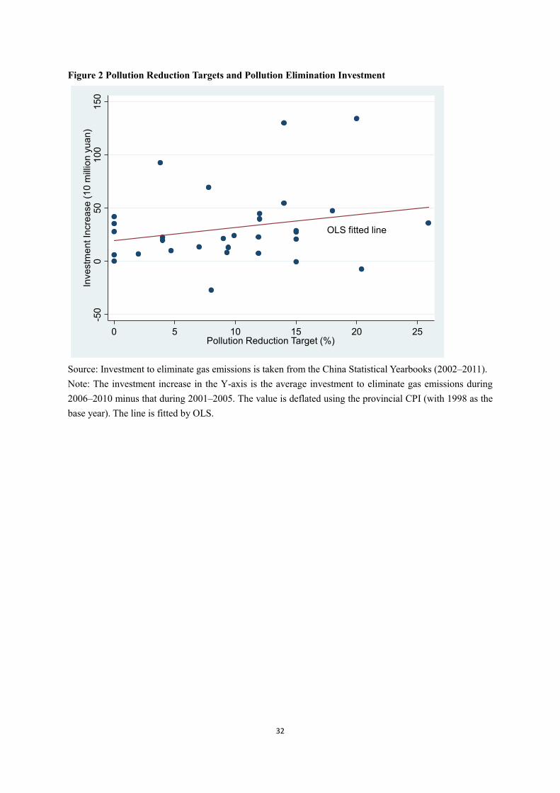
increased. Figure 2 shows the correlation between increased provincial

investment in eliminating gas emissions and pollution reduction targets.9 We

can see that provinces with high pollution reduction targets invested more after

the eleventh Five-Year Plan to reduce pollution, and their efforts brought returns.

9 The increase in provincial investment is the difference between the average values in 2006–

2010 versus 2001–2005. Provincial investment in eliminating gas emissions is taken from the

China Statistical Yearbook (2002–2011).

9

Total SO� emission decreased by roughly 14% from 25.5 million tons in 2005

to 21.9 million tons in 2010.10 Figure 3 shows the SO� emission trends for

provinces with pollution reduction targets above and below the median, with

greater SO� emission decreases after the start of the eleventh Five-Year Plan

for provinces with high pollution reduction targets.

Enforcement varied across the provinces. Figure 4 shows SO�

emissions for each province in 2005 and 2010. We can see that SO� emissions

in 2010 are lower than those in 2005 for most provinces, while a few have

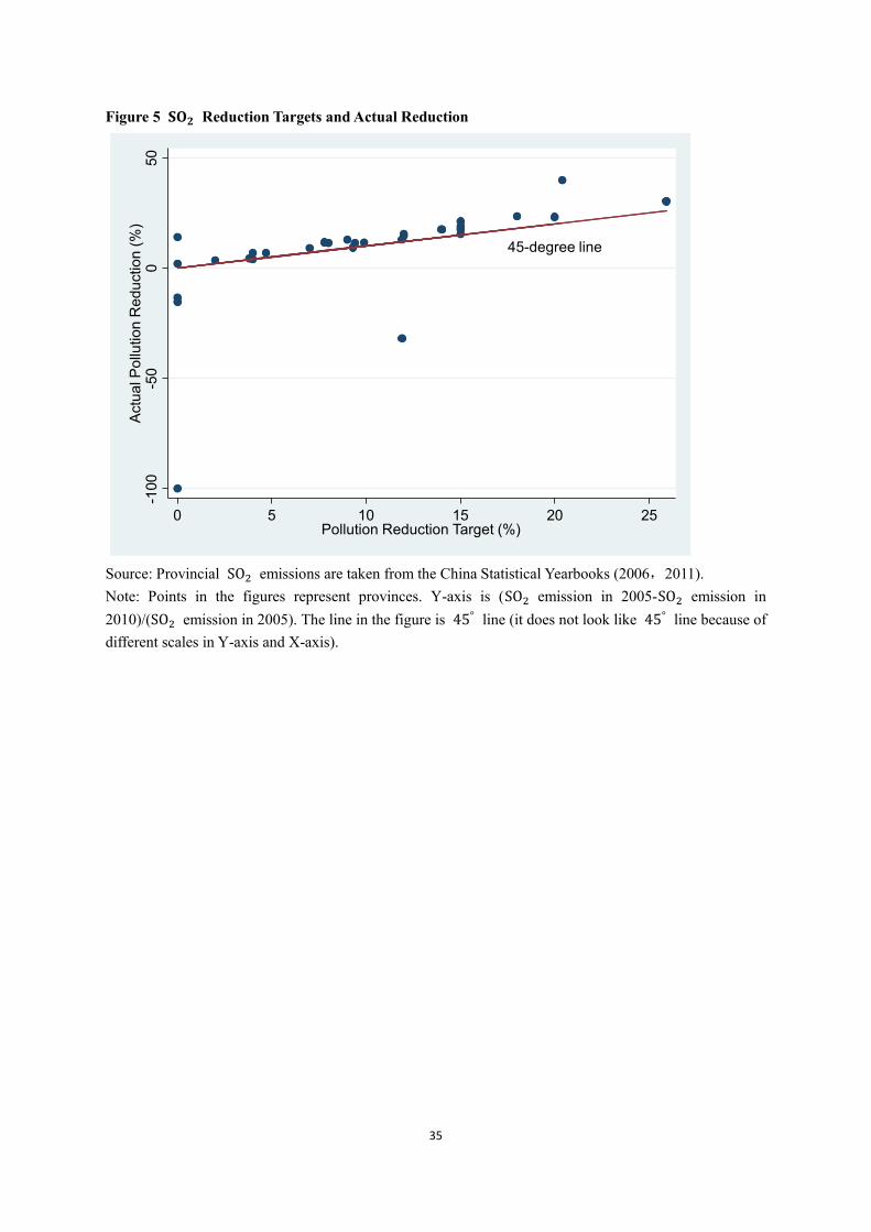
higher SO� emissions in 2010. Figure 5 shows the relation between the actual

SO� emission reductions and the targets. We can see that most provinces

achieved or even exceeded their targets, while a few did not.11

3. Data

The data on pollution reduction targets was collected from a document

named “Reply to Pollution Control Plan During the Eleventh Five-Year Plan,”

issued by the China State Council in 2006.12 Figure 1 shows the distribution of

the pollution reduction targets, which vary from 0 to more than 25% with a

mean and standard deviation of 9.645% and 6.808%, respectively. We obtain the

10 The total SO� emissions data is from the China Statistical Yearbook (2006 and 2011). 11

However, except for setting the SO� emission target in 2010 for electricity sector in each

province, there is no evidence showing that the central government had guidance for what industries or sub-provincial entities for local governments to target. It is reasonable to speculate that local governments would focus on pollution intensive industries or sub-entities. 12 This document lists total SO� emission for each province in 2005, SO� emission target

for each province in 2010, SO� emission target for electricity sector in each province in 2010, and the reduction percentage target for each province (which is what we use in the paper). Online Appendix Table 1 shows the details (translated from Chinese).

10

2-digit-industry level SO� emissions for 2003–2005 from the China Statistical

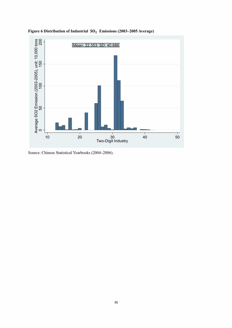
Yearbook (2004–2006).13 Figure 6 shows the three-year average (2003–2005)

of SO� emissions for industries. This also varies considerably, with a mean and

standard deviation of 22.353 thousand tons and 40.686 thousand tons,

respectively. We also obtain provincial SO� emissions and provincial

investment to eliminate gas pollution from China Statistical Yearbook

(2002-2011).

In this paper, we also use manufacturing firm data collected by the

National Bureau of Statistics of China (NBS). Every year, all SOEs and

non-SOEs with sales above RMB5 million (roughly $769,000) are required to

file a report with the NBS on their production activities, including their

accounting and financial information. This is the most comprehensive firm-level

dataset in China, and is used to calculate matrices for the national income

account and major statistics published in the China Statistical Yearbooks. The

data collected by this survey are widely used by researchers such as Brandt, Van

Biesebroeck, and Zhang (2012), Brandt et al. (2017), Yu (2014), Lu, Lu, and

Tao (2010), and Lu and Yu (2015).

The NBS assigns a four-digit Chinese industrial classification (CIC)

code to each firm. However, the classification system for the industry code

changed from GB/T 4754-1994 for 1995–2002 to GB/T 4754-2002 after 2002.

To achieve consistency among industry codes for the entire period, we convert

13 The industries used in our paper are listed in Table 2 of the online appendix.

11

them to GB/T 4754-1994. We then clean the data following the procedures in

the literature (Cai and Liu, 2009; Lu and Yu, 2015; Yu, 2014). All of the

monetary values are deflated to 1998 values. We use data from 2002 to 2009,

spanning four years before the eleventh Five-Year Plan (2002–2005) and four

years after the eleventh Five-Year Plan (2006–2009). Because the variations

used for identification are at the province-industry-year level, which are

discussed in more detail in Section 4, we collapse all firm level variables into

the mean of each province-industry-year cell. Finally, we have 7,137

province-industry-year cells generated from 2,109,196 firm level observations.

In this paper, we also use the ventilation coefficient, a variable based on

the product of wind speed and the mixing height, for each province. We use the

wind speed information at the 10-m height and the boundary layer height (used

to measure mixing height for the grid of 75°*75° cells) from the European

Center for Medium-Term Weather Forecasting ERA-interim dataset. We match

the ERA-interim dataset with the capital city of each province by its latitude and

longitude. The ventilation coefficient is the product of the wind speed and

boundary layer height for each cell. The ventilation coefficient we use is the

average coefficient from 1998 to 2004 for the nearest cells to the capital city of

each province.

Table 1 shows the summary statistics for the variables used in the

analysis. On average, 26.3% of the firms are exporters, with an export value of

17,640 thousand yuan and average fixed assets of 25,739 thousand yuan. The

12

average provincial policy intensity (measured by the SO� emission reduction

target) is 9.6%. The industrial SO� emissions (2003–2005 average) is 22.4

thousand tons, and the average ventilation coefficient is 1,747.

4. Empirical Strategy

Combining the variation in pollution reduction targets across provinces

and the before-and-after change, we can estimate the impact of environmental

regulations on firm exports using a difference-in-differences (DID) strategy.

However, a concern about the DID strategy is that some time-varying provincial

characteristics may be correlated with the outcome variable and the regressor at

the same time, leading to bias in our estimates.

In light of this concern, we exploit the fact that industries that have

different pollution intensities are affected differently, and carry out a

difference-in-difference-in-differences (DDD) strategy. In other words, we

combine three types of variation: the time variation (i.e., before and after the

start of the eleventh Five-Year Plan), the provincial variation (i.e., provinces

with high pollution reduction targets versus provinces with low targets), and the

industrial variation (i.e., more polluting versus less polluting industries).14 The

following regression is estimated:

�� = � ∗ ��(�� ) ∗ �� ∗ ��(��2�) + " � + # � + $�� + %� �

14 Another possibility is to explore the variation in city-level pollution within each province, that is, to combine the time variation, variation in provincial pollution reduction targets, and city level variation in pollution to estimate the effects. Unfortunately, we cannot find city-level pollution data.

13

(1).

Given that we exploit the variations over province-industry-year, we

collapse the variables and conduct the analysis at the provincial, 2-digit industry,

and year levels.15 �� is a vector including the proportion of exporting firms in

province p, industry i, and year t, and the natural logarithm form of the average

export value of exporters in province p, industry i, and year t (Ln(export� �)).

�� is the pollution reduction target for province p; �� is a dummy

variable equal to 0 for 2002–2005 and 1 for 2006–2009; ��2� is the average

SO� emissions from 2003 to 2005 for each industry; and %� � is an error term

with a mean equal to zero. To deal with heterogeneity and serial correlations, we

calculate the standard error by clustering over province-industry to allow for the

possible correlation of firms within the province-industry. In all of the

regressions, we use the number of firms in each province-industry-year cell as a

weight.16

The DDD strategy makes it feasible to control for the entire set of

province-year fixed effects (" �), province-industry fixed effects (# �), and

industry-year fixed effects ($�� ). In other words, we can control for all

time-invariant and time-varying provincial characteristics and all time-invariant

15 As we only have information on pollution intensity at the 2-digit industry level, we cannot exploit industrial variations at a more disaggregated level, which could lead to bias in our estimates. For example, if one sector includes one highly polluting industry but all of the rest are clean industries, our estimates will be downward biased, as the small change in export for clean industries could offset the change in exports for the highly polluting industry. 16 Each observation in our analysis is an average value for the province-industry-year cell. Therefore, a cell with more firms will be under-represented in the analysis. The number of firms in each province-industry-year cell is used as a weight for the representation of each cell. Stata syntax aweight is used.

14

and time-varying industry characteristics. We also control for any time-invariant

differences for industries in different provinces.

However, if the exports of heavily polluted industries were taken into

account when the provincial pollution reduction targets were being set, our

estimates would still be biased. To address this issue, we adopt an IV strategy.

Specifically, we use the ventilation coefficient as the IV for policy intensity.

According to the Box model (Jacobson, 2002), two variables determine

pollution dispersion. One is wind speed, as a faster wind speed helps the

horizontal dispersion of pollution, and the second is mixing height, which

influences the vertical dispersion of pollution. The ventilation coefficient is the

product of wind speed and mixing height. Higher ventilation coefficient values

mean faster dispersion of pollution, leading to a lower policy intensity in our

context. The ventilation coefficient has been widely used as an IV for

environmental policies in other studies (e.g., Broner, Bustos, and Carvalho,

2013; Cai et al., 2016; Hering and Poncet, 2014). We construct the ventilation

coefficient using the procedure described in Section 3.

To further check the validity of the empirical strategy, we conduct a

battery of sensitivity tests. These include checking for the existence of pre-trend

and expectation effects, controlling for the value-added tax reform, the 2008–

2009 financial crisis, and the 2008 Beijing Olympic Games, using firms in the

same province and industry that existed both before and after the eleventh

Five-Year Plan, and using alternative measures of policy intensity. In all of the

15

robustness checks, the IV strategy is used unless stated otherwise.17

5. Results

5.1. Main Results

As a benchmark, we first show the OLS estimates of Equation (1) in

Table 2. Column 1 shows the results using the proportion of exporters as the

outcome variable and column 2 shows Ln(export). Due to limited space, only

the coefficient of ��(�� ) ∗ �� ∗ ��(��2�) is presented. The

coefficients are -0.004 (column 1) and -0.042 (column 2), the former being

statistically significant at the 1% level and the latter at the 5% level.

OLS estimates could be biased if the exports of different industries in

different provinces were taken into account when setting provincial pollution

reduction targets. We therefore rely on the IV strategy, using the ventilation

coefficient as the IV for pollution reduction targets. Estimation results are

shown in Table 3.

Columns 1–2 in Table 3 report the first-stage results. Column 1 is for

proportion of exporters and column 2 is for Ln(export). The IV is a very strong

predictor of policy intensity with F-values of 313.7 and 184.5, respectively. The

second-stage results are shown in columns 3–4 of Table 3. We continue to find

significant negative effects of the eleventh Five-Year Plan on the probability of

firms exporting and export value, with coefficients of -0.005 (column 3) and

17 The first stage results are presented in the online-appendix.

16

-0.069 (column 4), respectively.

The results show that when the pollution reduction target is one standard

deviation above the mean, there are one percentage point fewer exporting firms

in industries with SO� emissions 10% above the mean and the value of exports

is 13% lower.18 Given the average number of firms per year (roughly 263,650)

and the average value of exports (17,640 thousand yuan), it means 2,637 fewer

firms exporting and a 2,293 thousand yuan reduction in export value.

5.2. Justification of Identification

Pre-existing Time Trends. Our estimates would be biased if different

time trends in the absence of the eleventh Five-Year Plan are correlated with

firm export behavior and our IV. To investigate this, we replace the post dummy

in Equation (1) with dummies for 2003–2009 (the base year is 2002) and use the

interactions of Ln(Ventilation), year dummies, and Ln(Industry SO2) as the

relevant IVs. The results are shown in columns 1 (proportion of exporters) and 2

(Ln(export)) in Table 4. None of the coefficients of the triple interaction

between 2003 and 2005 are significant, which validates our empirical strategy.19

18 The formula is ∆= �/ ∗ ��(��0123 + ��45) ∗ ��(��20123 ∗ (1 + 10%)) −

�/ ∗ ��(��0123) ∗ ��(��20123) ). Here, ∆ represents change in the proportion of

exporters or Ln(export), �/ is the estimated coefficient in equation (1), ��0123 is

average value of pollution reduction target, ��45is the standard deviation of pollution

reduction target, and ��20123is the average industry pollution level. 19

One might also be concerned that there could be some variables with different time trends

across industries and provinces. These variables might not affect exports immediately but

rather a few years later. If so, we should also see significant interaction coefficients during

2003–2005, as the aforementioned variables before 2003 could affect exports during 2003–

2005. However, Table 4 shows no significant interactions during 2003–2005, providing no

17

Expectation Effects. Firms in industries with more intense pollution in

provinces with higher reduction targets could have expected the event under

study and changed their behavior even before the eleventh Five-Year Plan.

However, the results in Table 4 suggest that the expectation effects do not exist

because none of the coefficients of the triple interaction between 2003 and 2005

are significant.20

Concurrent Events. If any other events during the period of the eleventh

Five-Year Plan affected different industries across provinces, our estimates

could be biased. Three such events stand out: the value-added tax reform, the

2008–2009 financial crisis, and the 2008 Beijing Olympic Games.

The value-added tax reform during the mid-2000s allowed firms in

specific industries (mainly heavy industries) in selected provinces to deduct the

purchase of fixed assets from their tax base (see Liu and Lu, 2015, and Chen,

He, and Zhang, 2017, for a detailed description of the background). This reform

significantly increased firm investment (Chen, He, and Zhang, 2017) and

therefore raised both the probability of firms exporting and the export value

(Liu and Lu, 2015). As heavy industries are more pollution intensive, our results

evidence of such variables. It is also possible that some other event during 2003–2005 could

have led to different time trends for firm exports in different polluting industries and different

provinces, and if this only affected exports a few years later, our estimates could be biased.

One such event is the tax reform during the mid-2000s discussed in Section 5.2. However, as

shown in Section 5.2, this reform does not affect our estimates. 20 One caveat we need to bear in mind is that, despite the statistical insignificance, the coefficients of the triple interaction terms in 2005 could still indicate that some changes might have started to be made in 2005. For example, the positive (but insignificant) coefficient of the triple interaction term in 2005 for Ln(export) could suggest that exporters might export more in expectation of higher production costs in the next year.

18

may be biased upward. To address this concern, we include the log value of

fixed assets in the regression. As shown in column 1 of Panel A in Table 5

(using the proportion of exporters as the outcome variable), the coefficient of

the triple interaction is still -0.005 and significant at the 1% level. The

coefficient of the triple interaction in column 1 of Panel B (using Ln(export) as

the outcome variable) is -0.070 and also significant at the 1% level. Both are

consistent with those shown in columns 3–4 in Table 3.

During the 2008–2009 financial crisis, firm exports declined

dramatically (Ma, Shi, and Sivadasan, 2016). If the impact of the financial crisis

was larger for firms in industries with more intensive pollution in provinces

with higher pollution reduction targets, our estimates may be biased. To

investigate the effects of the financial crisis, we drop 2008 and 2009 from the

sample, and the results are shown in column 2 of Table 5. We can see that in

Panel A (using the proportion of firms as the outcome variable) the coefficient

of the triple interaction term is -0.004 and significant at the 1% level, which is

similar to our main estimate. In Panel B (using Ln(export) as outcome variable),

the coefficient of the triple interaction is -0.073 and significant at the 1% level,

also similar to our main estimate.

The Chinese government exerted considerable effort to reduce pollution

in Beijing during the 2008 Olympic Games. This might have especially affected

firms in industries with heavy pollution in provinces around Beijing. Indeed, He,

Fan, and Zhou (2016) show that not only Beijing but also Hebei, Tianjin, Shanxi,

19

Neimenggu, and Liaoning were affected. To investigate the potential effects of

this event, we exclude firms in the provinces affected by the Olympic Games

from 2007 and 2008 (column 3 of Table 5). The coefficients of the triple

interaction for both outcome variables remain similar to the main results shown

in Table 3.

The preceding results suggest that these three concurrent events do not

affect our estimates.

Firms Existing Before and After the Five-year Plan. Tougher

environmental policies following the Five-Year Plan may have induced firms to

exit the market or move to other provinces and industries, leading to bias in our

estimates. We therefore restrict the sample to firms existing within the same

industry and province both before and after the Five-Year Plan and conduct the

same analysis. The results are shown in Table 6, where the coefficient of the

triple interaction remains robust.

Alternative Measurement for Policy Intensity. In the main analysis, we

use the targeted pollution reduction percentage to measure policy intensity. One

might be concerned about the precision of this measurement, as even a small

percentage could represent a large burden for provinces with heavy pollution.

We then construct the amount of expected pollution reduction by multiplying

the percentage by the emission levels in 2005 (scaled by GDP in 2005 to

account for the different economy sizes among provinces). When we re-estimate

equation (1) using this newly constructed variable for policy intensity, the

20

results shown in Table 7 remain robust.

5.4. Heterogeneous Effects

In addition to the average effects, we investigate how the effects differ in

terms of firm ownership and location. Once again, the IV strategy is used, and

the results are shown in Table 8.21

Columns 1–4 in Table 8 show the effects for SOEs, foreign invested

firms, Hong Kong-Marco-Taiwan invested firms, and domestic non-SOE firms.

We see that the coefficients of the triple interaction are not significant for SOE

firms, whether the outcome variable is the proportion of exporters (Panel A) or

Ln(export) (Panel B). These results are consistent with Hering and Poncer

(2014). This could be because of the preferential treatment of SOEs in China.

Indeed, as Huang (2003) points out, because the Chinese government

systematically favors SOEs both financially and legally, SOEs have better

access to finance (Dollar and Wei, 2007; Boyreau-Debray and Wei, 2004). As

Hering and Poncer (2014) argue, better access to finance makes it easier for

SOEs to adopt advanced technology such that with reduced obligations to

comply with stricter regulations, SOEs can continue to produce and export.

Columns 5–7 in Table 8 show the effects for firms in the eastern, central,

and western parts of China, respectively.22 The effects are significant for firms

21 The first stage results are shown in the online appendix. 22 The eastern part of China includes Beijing, Tianjin, Hebei, Liaoning, Shanghai, Jiangsu, Zhejiang, Fujian, Shandong, Guangdong, and Hainan provinces. The central part of China includes Shanxi, Jilin, Heilongjiang, Anhui, Jiangxi, Henan, Hubei, and Hunan provinces.

21

in the east for both outcome variables. The magnitude is also larger for firms in

the east. However, most of the effects on firms in the central and western areas

are not significant. A possible explanation is that because pollution is most

severe in the eastern part of China, the pollution reduction targets there are

highest, and therefore implementation of the pollution reduction policy could be

the strictest there compared with the central and western regions.23

6. What Causes the Declined Probability of Firm Exporting?

In this section, we investigate the channels through which the pollution

reduction policy affected the probability that a firm would export. Specifically,

we investigate whether this policy induced incumbent exporters to exit the

export market and/or prevented non-exporters from entering the export market.

We define incumbent exporters as firms that exported at least once

before the start of the eleventh Five-Year Plan, and non-exporters as firms that

never exported before the eleventh Five-Year Plan. We then obtain a panel of

exporters and non-exporters, respectively. As in the previous regressions, we

collapse individual firms to the province-industry-year level and use the IV

strategy. The regression results are shown in Table 9.

Column 1 in Table 9 applies to incumbent exporters. The coefficient of

The western part of China includes Neimenggu, Guangxi, Chongqing, Sichuan, Guizhou, Yunnan, Tibet, Shaanxi, Gansu, Qinghai, Ningxia, and Xinjiang provinces. 23 The average reduction targets are 14.4% for provinces in the eastern part of China, 7.8% for provinces in the central part of China, and 6.5% for provinces in the western part of China.

22

the triple interaction is -0.002 and not significant. Column 2 in Table 9 applies

to non-exporters, and here the triple interaction coefficient is -0.003 and

significant at the 5% level. The results show that the pollution reduction policy

decreased the probability of non-exporters entering the export market, but did

not affect the probability of incumbent exporters exiting the export market. As

shown in Melitz (2003), firms had to pay fixed costs to enter the export market.

Stricter environmental policies reduced the ability of non-exporters to pay these

costs, but may not have induced exporters to exit the export market as they had

already paid these costs. This may explain why the pollution reduction policies

had different effects on exporters and non-exporters.

One might still be interested in how non-exporters responded to the

stricter environmental regulations. They could reduce their production output

and/or introduce more advanced technology and equipment. Because we do not

have data on the more advanced technology or equipment adopted by firms, we

can only investigate how the regulations affected the output of non-exporters.

The results in column 3 of Table 9 show that reducing output may have been

one response of non-exporters to the stricter environmental regulations.

7. Conclusion

We investigate the effects of domestic environmental regulations on the

export behavior of firms using China’s eleventh Five-Year Plan. Applying the

DDD identification strategy, we find that stricter environmental regulations

23

reduced the likelihood that firms would export and also reduced export volume.

Several robustness checks confirm our findings. We also find that SOE firms

and firms located in the middle and western part of China were least affected.

Finally, we show that the reduced probability of non-exporters entering the

export market was the main driving force for the reduced probability of firms

exporting.

It would be interesting to investigate whether exporters eventually exited

the export market or bounced back after adapting to the regulations, as such

long-term effects have important implications for evaluating current policy and

future policy making. This is a potential topic for future research when the

relevant data are available.

In developing countries like China, governments are investing large

amounts of resources to reduce the increasingly severe pollution. While such

investment has many benefits, our study shows that it can also bring extra costs

to manufacturing firms. Policymakers therefore need to take these negative

effects into account in future policymaking.

24

References

Antweiler, Werner, Brian R. Copeland, and M. Scott Taylor, (2001). Is free trade

good for the environment? American Economic Review, Vol. 91, No. 4,

877-908.

Becker, Randy, and J. Vernon Henderson, (2000). Effects of air quality

regulations on polluting industries. Journal of Political Economy, Vol. 108, No.

2, 379-421.

Blonigen, Bruce A., and Miao Wang, (2004). Inappropriate pooling of wealthy

and poor countries in empirical FDI studies. NBER Working Paper No. 10378.

Boyreau-Debray, Genevieve, and Shang-jin Wei. (2004). Can China grow faster?

A diagnosis on the fragmentation of the domestic capital market. IMF working

paper, 04/76.

Brandt, Loren, Johannes Van Biesebroeck, and Yifan Zhang. (2012) Creative

accounting or creative destruction: Firm level productivity growth in Chinese

manufacturing. Journal of Development Economics, Vol. 97, No. 2, 339-351.

Brandt, Loren, Johannes Van Biesebroeck, Luhang Wang, and Yifan Zhang,

(2017). WTO accession and performance of Chinese manufacturing firms.

American Economic Review, 107(9), 2784-2820.

Broner, Fernando, Paula Bustos, and Vasco M. Carvalho, (2013). Sources of

comparative advantage in polluting industries. Working Paper.

Cai, Hongbin, and Qiao Liu, (2009). Competition and corporate tax avoidance:

Evidence from Chinese industrial firms. Economic Journal, Vol. 119, 537,

25

764-795.

Cai, Xiqian, Yi Lu, Mingqin Wu, and Linhui Yu, (2016). Do environmental

regulations drive away inbound foreign direct investment? Evidence from a

quasi-natural experiment in China. Journal of Development Economics, Vol.

123, 73-85.

Chen, Y. A., M. Ebenstein, M. Greenstone, and H. Li, (2013). Evidence on the

impact of sustained exposure to air pollution on life expectancy from China’s

Huai River policy. Proceedings of National Academy of Science USA, 110(32),

12936-12941.

Chen, Yuyu, Zongyan He, and Lei Zhang, (2017). The effect of investment tax

incentives: Evidence from China’s value-added tax reform. International Tax

and Public Finance, July, 1-23.

China Statistical Yearbook (2002-2011). China Statistical Press, Beijing.

Chung, Sunghoon, (2014). Environmental regulation and foreign direct

investment: Evidence from South Korea. Journal of Development Economics,

Vol. 108, 222-236.

Copeland, Brian R., and M. Scott Taylor, (2004). Trade, growth, and the

environment. Journal of Economic Literature, Vol. 42, No. 1, 7-71.

Dean, Judith M., Mary E. Lovely, and Hua Wang, (2009). Are foreign investors

attracted to weak environmental regulations? Evaluating the evidence from

China. Journal of Development Economics, 90, 1-13.

Dollar, David, and Shang-jin Wei, (2007). Das (Wasted) Kapital: Firm

26

ownership and investment efficiency in China. IMF working paper 07/9.

Ederington, Josh, and Jenny Minier, (2003). Is environmental policy a

secondary trade barrier? An empirical analysis. Canadian Journal of Economics,

Vol. 36, No. 1, 137-154.

Erdogan, Ayse M., (2014). Foreign direct investment and environmental

regulations: A survey, Journal of Economic Surveys, Vol. 28, 943-955.

Gan, Li, Manuel Hernandez, and Shuang Ma, (2016). The higher costs of doing

business in China: Minimum wages and firms’ export behavior, Journal of

International Economics, Vol. 100, No. C, 81-94.

Greenstone, M., and R. Hanna, (2011). Environmental regulations, air and water

pollution, and infant mortality in India. NBER Working Paper 17210.

Grossman, Gene M., and Alan B. Krueger, (1993). Environmental impacts of a

North American free trade agreement. NBER Working Paper 3914.

Hanna, Rema, (2011). US environmental regulation and FDI: Evidence from a

panel of US-based multinational firms. American Economic Journal: Applied

Economics, Vol. 2, 158-189.

Hanna, R., and P. Oliva, (2011). The effect of pollution on labor supply:

Evidence from a natural experiment in Mexico. NBER Working Paper 17302.

He, Guojun, Maoyong Fan, and Maigeng Zhou, (2016). The effect of air

pollution on mortality in China: Evidence from the 2008 Beijing Olympic

Games. Journal of Environmental Economics and Management, Vol. 79, pp.

18-39.

27

Henderson, J. Vernon, (1996). Effects of air quality regulation. American

Economic Review, Vol. 86, No. 4, 789-813.

Hering, Laura, and Sandra Poncet, (2014). Environmental policy and exports:

Evidence from Chinese cities. Journal of Environmental Economics and

Management, Vol. 68, 296-318.

Huang, Yasheng, (2003). One country, two systems: Foreign-invested

enterprises and domestic firms in China. China Economic Review, 14(4),

404-416.

Jacobson, M., (2002). Atmospheric pollution: History, science and regulation.

Cambridge, Cambridge University Press.

Jaffe, Adam B., Steven R. Peterson, Paul R. Portney, and Robert N. Stavins,

(1995). Environmental regulation and the competitiveness of U.S.

manufacturing: What does the evidence tell us? Journal of Economic Literature,

Vol. 33, No. 1, 132-163.

Javorcik, Beata S., and Shang-jin Wei, (2004). Pollution havens and foreign

direct investment: Dirty or popular myth? Contributions to Economic Analysis

& Policy. Vol. 3, No. 8.

Jeppesen, Jim, John A. List, and Henk Folmer, (2002). Environmental

regulations and new plant location decisions: Evidence from a meta-analysis.

Journal of Regional Science, Vol. 42, 19-49.

Kellenberg, Derek, (2009). An empirical investigation of the pollution haven

effect with strategic environment and trade policy. Journal of International

28

Economics, Vol. 78, No. 2, 242-255.

Keller, Wolfgang, and Arik Levinson, (2002). Pollution abatement costs and

foreign direct investment inflow to U.S. states. Review of Economics and

Statistics, Vol. 84, 691-703.

Levinson, Arik, (1996). Environmental regulations and manufacturer’s location

choice: Evidence from the census of manufacturers. Journal of Public

Economics, Vol. 62, 5-29.

Levinson, Arik, and M. Scott Taylor, (2008). Unmasking the pollution haven

effect. International Economic Review, Vol. 49, No. 1, 223-254.

List, John A., and Catherine Y. Co, (2000). The effects of environmental

regulations on foreign direct investment. Journal of Environmental Economics

and Management, Vol. 40, 1-20.

List, John A., Daniel L. Millimet, Per G. Fredriksson, and W. Warren McHone,

(2003). Effects of environmental regulations on manufacturing plant births:

Evidence from a propensity score matching estimator. Review of Economics and

Statistics, Vol. 85, 944-952.

Liu, Qing, and Yi Lu, (2015), Firm investment and exporting: Evidence from

China’s value-added tax reform. Journal of International Economics, Vol. 97,

No. 2, 392-403.

Lu, Jiangyong, Yi Lu, and Zhigang Tao, (2010). Exporting behavior of foreign

affiliates: Theory and evidence. Journal of International Economics, Vol. 82,

No. 2, 197-205.

29

Lu, Yi, and Linhui Yu. (2015), Trade liberalization and markup dispersion:

Evidence from China’s WTO accession. American Economic Journal: Applied

Economics, Vol. 7, No. 4, 221-253.

Ma, Yueyuan, Xinzheng Shi, and Jagadeesh Sivadasan, (2016). Spillover effects

of foreign demand shock: Chinese experience in 2008-2009 crisis. Working

Paper.

Melitz, J. Marc, (2003). The impact of trade on intra-industry reallocations and

aggregate industry productivity. Econometrica, Vol. 71, No. 6, 1695-1725.

Millimet, Daniel L., and Joyjit Roy, (2016). Empirical tests of the pollution

haven hypothesis when environmental regulation is endogenous. Journal of

Applied Econometrics, Vol. 31, 652-677.

Nunn, Nathan, and Daniel Trefler, (2014). Domestic institutions as a source of

comparative advantage, Chapter 5. Handbook of International Economics,

Volume 4. Netherlands: North Holland Publishing Company.

State Environment Protection Administration, (2006). A letter on signing up

liability contracts of major pollutants. Beijing (in Chinese).

Taylor, M. Scott, (2004). Unbundling the pollution haven hypothesis. Advances

in Economic Analysis & Policy, Vol. 4, Issue 2, Article 8.

Tobey, James A., (1990). The effects of domestic environmental policies on

patterns of world trade: An empirical test. KYKLOS, Vol. 43, Issue 2, 191-209.

Wang, Alex L., (2013). The search for sustainable legitimacy: Environmental

law and bureaucracy in China. Harvard Environmental Law Review, vol. 37,

30

365-440.

Xu, Yuan, (2011). The use of a goal for SO� mitigation planning and

management in China’s 11th Five-Year Plan. Journal of Environmental Planning

and Management, Vol. 54, No. 6, 769-783.

Yang, Xinxing, Qingxian Gao, Zhenyuan Jiang, Zhenhai Ren, Fu Chen, Fahe,

Chai, and Zhigang Xue, (1998). Research on the transportation and precipitation

regular pattern of sulfur pollutants in China. Research of Environmental

Sciences, Vol. 11, No. 4, 27-34. (in Chinese).

Yang, Xinxing, Qingxian Gao, Jinzhi Qv, and Zhenyuan Jiang, (1999). The

exploration and initial assessment of total amount control method for SO�

emissions in China. Research of Environmental Sciences, Vol. 12, No. 6, 17-20.

(in Chinese).

Yu, Miaojie. (2015) Processing trade, tariff reductions and firm productivity:

Evidence from Chinese firms. Economic Journal, Vol. 125 (June), 943-988.

31

Figure 1 Distribution of Pollution Reduction Targets

Source: Pollution targets are taken from the document “Reply to Pollution Control Plan During the

Eleventh Five-Year Plan,” issued by the China State Council in 2006.

Note: The province names in the x-axis are sorted by their codes assigned by National Bureau of Statistics.

Mean: 9.645; SD: 6.8080

510

15

20

25

Po

llutio

n R

ed

uctio

n T

arg

et (%

)

Be

ijing

Tia

njin

He

bei

Sh

anxi

Ne

ime

nggu

Lia

on

ing

Jili

nH

eilo

ng

jiang

Sh

an

ghai

Jia

ngsu

Zh

ejia

ng

An

hui

Fu

jian

Jia

ngxi

Sh

an

dong

He

nan

Hu

bei

Hu

nan

Gu

an

gd

ong

Gu

an

gxi

Ha

inan

Ch

on

gqin

gS

ich

uan

Gu

izh

ou

Yu

nn

an

Tib

et

Sh

aa

nxi

Ga

nsu

Qin

ghai

Nin

gxi

Xin

jiang

Province

32

Figure 2 Pollution Reduction Targets and Pollution Elimination Investment

Source: Investment to eliminate gas emissions is taken from the China Statistical Yearbooks (2002–2011).

Note: The investment increase in the Y-axis is the average investment to eliminate gas emissions during

2006–2010 minus that during 2001–2005. The value is deflated using the provincial CPI (with 1998 as the

base year). The line is fitted by OLS.

OLS fitted line

-50

050

100

150

Inve

stm

en

t In

cre

ase

(1

0 m

illio

n y

ua

n)

0 5 10 15 20 25Pollution Reduction Target (%)

33

Figure 3 9:; Emissions

Source: Provincial SO� emissions are taken from the China Statistical Yearbooks (2002–2011).

Note: Provinces with pollution reduction targets higher than the median (9.4%) are referred to as provinces

with high targets. Provinces with pollution reduction targets below the median (9.4%) are referred to as

provinces with low targets. The vertical line in the figure denotes the start of the eleventh Five-Year Plan.

40

60

80

100

120

SO

2 E

mis

sio

n (

10

,00

0 to

ns)

2001 2002 2003 2004 2005 2006 2007 2008 2009 2010Year

Provinces with high targets Provinces with low targets

34

Figure 4 9:; Emissions in 2005 and 2010

Source: Provincial SO� emissions are taken from the China Statistical Yearbooks (2006，2011).

Note: Points in the figures represent provinces. The line in the figure is the 45° line.

45-degree line

050

100

150

20

0S

O2

Em

issio

ns in

20

10

(1

0,0

00

to

ns)

0 50 100 150 200SO2 Emissions in 2005 (10,000 tons)

35

Figure 5 9:; Reduction Targets and Actual Reduction

Source: Provincial SO� emissions are taken from the China Statistical Yearbooks (2006，2011).

Note: Points in the figures represent provinces. Y-axis is (SO� emission in 2005-SO� emission in

2010)/(SO� emission in 2005). The line in the figure is 45° line (it does not look like 45° line because of

different scales in Y-axis and X-axis).

45-degree line

-100

-50

050

Actu

al P

ollu

tio

n R

ed

uctio

n (

%)

0 5 10 15 20 25Pollution Reduction Target (%)

36

Figure 6 Distribution of Industrial 9:; Emissions (2003–2005 Average)

Source: Chinese Statistical Yearbooks (2004–2006).

Mean: 22.353; SD: 40.686

050

100

150

200

Ave

rag

e S

O2

Em

issio

n (

20

03

-20

05

), u

nit: 1

0,0

00

to

ns

10 20 30 40 50Two-Digit Industry

37

Table 1 Summary Statistics

Mean S.D. OBS

Panel A. Province-industry-year level

Exporter 0.263 0.186 7137

Exports (1,000 yuan) 17640.213 38257.866 6039

Fixed assets (1,000 yuan) 25738.953 41223.838 7137

Panel B. Province level

Provincial pollution reduction target (%) 9.645 6.808 31

Ventilation coefficient 1746.680 564.939 31

Panel C. Two-digit industry level

Industry SO2 emissions (2003–2005 average) (1,000 tons) 22.353 40.686 30

Notes:

(1) The number of firms in each province-industry-year cell is used as the weight for the mean and standard

deviation in Panel A.

(2) Exports include only province-industry-year cells with positive export values.

38

Table 2 Impact of Environmental Regulations on Firm Exports (OLS Estimates)

(1) (2)

Dependent Variable: Proportion of exporters Average Ln(export)

Ln(Policy intensity)*Post*Ln(Industry SO2) -0.004*** -0.042**

(0.001) (0.020)

Year-Province FE Yes Yes

Year-Industry FE Yes Yes

Province-Industry FE Yes Yes

Observations 7,137 6,039

R-squared 0.984 0.889

Notes:

(1) Standard errors in parentheses are calculated by clustering over province-industry. The

number of firms in the cell of province-industry-year is used as a weight.

(2) ***, **, and * represent the significance levels at 1%, 5%, and 10%, respectively.

(3) Variables are collapsed to the province-industry-year level.

39

Table 3 Impact of Environmental Regulations on Firm Exports (IV Estimates)

(1) (2)

(3) (4)

First Stage

Second Stage

Dependent Variable: Ln(Policy intensity)*Post*Ln(Industry

SO2)

Proportion of

exporters

Average

Ln(export)

Ln(Ventilation)*Post*Ln(Industry SO2) -3.932*** -4.503***

(0.222) (0.331)

Ln(Policy intensity)*Post*Ln(Industry SO2)

(Ln(Ventilation)*Post*Ln(Industry SO2) as IV) -0.005*** -0.069***

(0.001) (0.021)

Year-Province FE Yes Yes Yes Yes

Year-Industry FE Yes Yes Yes Yes

Province-Industry FE Yes Yes Yes Yes


7,137 6,039

R-squared 0.984 0.975

0.984 0.888

F-test 313.7 184.5

Notes:

(1) Robust standard errors in parentheses are calculated by clustering over province-industry. The number of firms in the

province-industry-year cell is used as a weight.


(3) Variables are collapsed to province-industry-year level.

40

Table 4 Testing Pre-existing Time Trends

(1) (2)

Dependent Variable: Proportion of exporters

Average

Ln(export)

Ln(Policy intensity)*Year2003 Dummy*Ln(Industry SO2)

(Ln(Ventilation)*Year2003 Dummy*Ln(Industry SO2) as IV) -0.000 -0.004

(0.001) (0.006)


(Ln(Ventilation)*Year2004 Dummy*Ln(Industry SO2) as IV) 0.002 -0.010

(0.001) (0.008)


(Ln(Ventilation)*Year2005 Dummy*Ln(Industry SO2) as IV) -0.001 0.014

(0.001) (0.016)


(Ln(Ventilation)*Year2006 Dummy*Ln(Industry SO2) as IV) -0.003*** -0.082***

(0.001) (0.023)



(0.001) (0.017)



(0.001) (0.018)



(0.002) (0.018)





R-squared 0.984 0.888

Notes:

(1) Standard errors in parentheses are calculated by clustering over province-industry. The number of firms in

the province-industry-year cell is used as a weight.



41

Table 5 Testing for Concurrent Events

(1) (2) (3)

Value added tax reform Financial crisis 2008 Beijing Olympic Games

Panel A: Proportion of exporters


(Ln(Ventilation)*Post*Ln(Industry SO2) as IV) -0.005*** -0.004*** -0.004***

(0.001) (0.001) (0.001)

Ln(fixed asset) 0.018***

(0.004)

Year-Province FE Yes Yes Yes

Year-Industry FE Yes Yes Yes

Province-Industry FE Yes Yes Yes

Observations 7,137 5,384 6,787

R-squared 0.985 0.986 0.985

Panel B: Average Ln(export)


(Ln(Ventilation)*Post*Ln(Industry SO2) as IV) -0.070*** -0.073*** -0.065***

(0.021) (0.023) (0.021)

Ln(fixed asset) 0.192***

(0.026)





R-squared 0.891 0.897 0.893

Notes: (1) Standard errors in parentheses are calculated by clustering over province-industry. The number of firms in the cell

of province-industry-year is used as weight.



(4) In column 2, samples from 2008 and 2009 are excluded. In column 3, samples from 2007 and 2008 in provinces affected

by the Olympic Games, including Beijing, Tianjin, Hebei, Shanxi, Neimenggu and Liaoning, are excluded.

42

Table 6 Robustness Check Using Firms Existing in the Same Industry and Province Before and After

(1) (2)

Proportion of exporters

Average

Ln(export)



(0.001) (0.022)





R-squared 0.984 0.887

Notes:

(1) Standard errors in parentheses are calculated by clustering over province-industry. The number of firms

in the province-industry-year cell is used as a weight.

(2) ***, **, and * represent the significance levels at 1%, 5%, and 10% respectively.


43

Table 7 Impact of Environmental Regulations on Firm Exports Using Alternative Policy Intensity Measurement

(1) (2)

(3) (4)

First Stage

Second Stage

Dependent Variable: Ln(Policy intensity

II)*Post*Ln(Industry SO2)

Proportion of

exporters

Average

Ln(export)

Ln(Ventilation)*Post*Ln(Industry SO2) -0.296*** -0.307***

(0.030) (0.036)

Ln(Policy intensity II)*Post*Ln(Industry SO2)


(0.013) (0.391)

Year-Province FE Yes Yes Yes Yes

Year-Industry FE Yes Yes Yes Yes

Province-Industry FE Yes Yes Yes Yes


7,137 6,039

R-squared 0.922 0.915

0.984 0.882

F-test 95.31 71.01

Notes: (1) Robust standard errors in parentheses are calculated by clustering over province-industry. The number of firms in the cell

of province-industry-year is used as weight.



(4) Policy intensity II is the amount of expected SO� emission reduction scaled by GDP. The amount of expected SO� emission

reduction is calculated as the pollution reduction target multiplied by the SO� emission level in 2005.

44

Table 8 Heterogeneous Tests

(1) (2) (3) (4) (5) (6) (7)

By Ownership By Region

SOE FDI HMT Non-SOE East Central West

Panel A: Proportion of exporters

Ln(Policy intensity)*Post*Ln(Industry SO2) -0.001 -0.005*** -0.003 -0.003*** -0.009*** -0.000 0.001

(Ln(Ventilation)*Post*Ln(Industry SO2) as IV) (0.001) (0.002) (0.000) (0.001) (0.001) (0.002) (0.002)

Year-Province FE Yes Yes Yes Yes Yes Yes Yes

Year-Industry FE Yes Yes Yes Yes Yes Yes Yes

Province-Industry FE Yes Yes Yes Yes Yes Yes Yes

Observations 6,697 5,557 5,357 6,908 2,604 1,897 2,636

R-squared 0.925 0.914 0.939 0.976 0.985 0.971 0.902

Panel B: Average Ln(export)

Ln(Policy intensity)*Post*Ln(Industry SO2) 0.006 -0.043*** -0.027** -0.089*** -0.292*** -0.105* 0.024

(Ln(Ventilation)*Post*Ln(Industry SO2) as IV) (0.018) (0.016) (0.011) (0.027) (0.050) (0.061) (0.023)

Year-Province FE Yes Yes Yes Yes Yes Yes Yes

Year-Industry FE Yes Yes Yes Yes Yes Yes Yes

Province-Industry FE Yes Yes Yes Yes Yes Yes Yes

Observations 4,282 4,447 3,827 5,428 2,470 1,730 1,839

R-squared 0.769 0.863 0.827 0.832 0.836 0.897 0.773

Notes: (1) Standard errors in parentheses are calculated by clustering over province. The number of firms in the province-industry-year

cell is used as a weight.



45

Table 9 Testing Channels

(1) (2)

(3)

Proportion of exporters in province-industry-year

Ln(Total

output)

Exporters Non-Exporters Non-Exporters

Ln(Policy intensity)*Post*Ln(Industry SO2) -0.002 -0.003** -0.012***

(Ln(Ventilation)*Post*Ln(Industry SO2) as IV) (0.001) (0.001) (0.004)





R-squared 0.936 0.886 0.954

Notes: (1) Standard errors in parentheses are calculated by clustering over province. The number of firms in the

province-industry-year cell is used as a weight.


Documents

Environmental Regulation and Firm Exports: Evidence from ...crm.sem.tsinghua.edu.cn/UploadFiles/File/201711/20171109115442593.… · In this paper, we take advantage of China’s