AGD Landscape & Environment 2 (2) 2008. 91-108.

91

ENVIRONMENTAL OBJECTIVE ANALYSIS, RANKING AND CLUSTERING OF HUNGARIAN CITIES LÁSZLÓ MAKRA AND ZOLTÁN SÜMEGHY Department of Climatology and Landscape Ecology, University of Szeged, H-6701 Szeged, P.O.B. 653, Hungary; E-mail: makra@geo.u-szeged.hu; sumeghy@geo.u-szeged.hu; Abstract The aim of the study was to rank and classify Hungarian cities and counties according to their environmental quality and level of environmental awareness. Ranking of the Hungarian cities and counties are represented on their „Green Cities Index” and „Green Counties Index” values. According to the methodology shown in Part 1, cities and counties were grouped on different classification techniques and efficacy of the classification was analysed. However, they did not give acceptable results either for the cities, or for the counties. According to the parameters of the here mentioned three algorithms, reasonable structures were not found in any clustering. Clusters received applying algorithm fanny, though having weak structure, indicate large and definite regions in Hungary, which can be circumscribed by clear geographical objects. Keywords: green Indices; ranking; clustering; SPSS-software; R-language 1. Introduction In Hungary, 236 cities accounting for 65.7% of the country’s population were registered on January 1, 2001. Environmental factors in cities such as housing, transportation, air quality and public green space, etc., are important to the quality of life (Kerényi, 1995). But which cities have cleaner air, more urban parkland, or more pleasant climate? Which do a better job at organising traffic systems, waste management or public sanitation? Which cities are wasteful in their use of water or energy? To answer these questions, at least at a preliminary level, the so-called “Green Cities Index”, which ranks cities on several environmental criteria, was developed (Cutter, 1992). 2. Materials and Methods Seven different categories of environmental indicators ranging from water consumption to air quality were included in the Green Cities Index. Specific measures within each category were selected on the basis of data availability. Some related measures were combined to yield new, composite measures. Altogether 25 indicators were considered initially but only 19 were retained (Publications of the

92

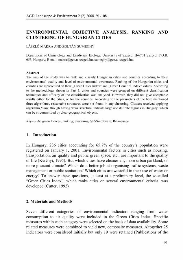
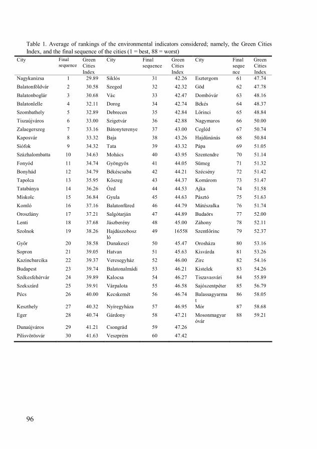
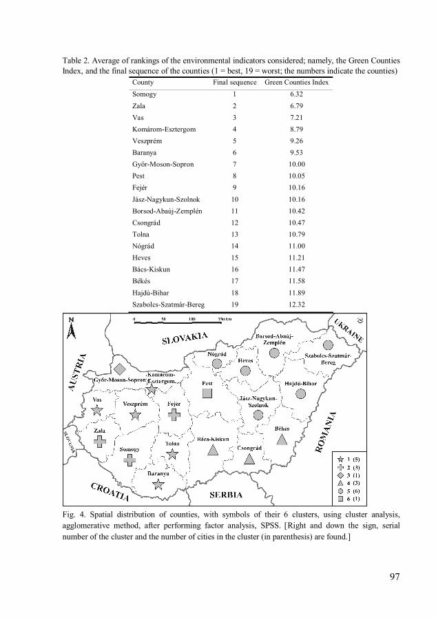
Central Statistical Office 2000; Statistical Year Books of the Hungarian counties 2000; Statistical Year Book of Budapest 2000;Vaskövi, 2000). The Green City Index is derived as follows (a) The statistics on each indicator for each city was compiled from the Year books. (b) Each indicator element is represented with a serial number (1 – 19). (c) For each indicator element, cities were ranked from the most environmentally friendly (1) to least friendly (88) based on their statistics as determined in step (a). These ranks represent city scores on each indicator. (d) The rank scores achieved for each city over the 19 indicator elements were averaged. The resulting figure is the City Green Index (column 3, Table 1). (e) Finally, the Green City Indices were ranked to yield the Final Sequence (column 2, Table 1). The Final Sequence (FS) places the cities in rank order from the best (1) to the worst (88) based on step (d). FS is a rank of ranks. 3. Results 3.1. Ranking Cities The final sequence of the cities shows some surprising results (Table 1). Nagykanizsa, near the Hungarian-Croatian border, is the highest-ranked city. It is followed by settlements around Lake Balaton: Balatonföldvár (2), Balatonboglár (3) and Balatonlelle (4). Among the major cities, Szombathely (5), Zalaegerszeg (7) and Kaposvár (8) are stand out (Table 1). Mosonmagyaróvár (88), Mór (87) and Balassagyarmat (86) are the worst ranked cities (Table 1) inspite of their relatively good rank in a number of indicators. Summing up, no city is found consistently either at the top or the bottom half of the rankings on all environmental indicators. All cities in Hungary are characterised by a mix of favourable and less favourable environmental quality. Environmental quality of Hungarian cities is best in the western and southern parts of Transdanubia, where Green Cities Index values are smallest. There are no clear regional patterns in the rest of the country (Fig. 1). Counties According to the final rank order of the counties (Table 2), Somogy is the greenest county of Hungary. Though it is almost the most wasteful in water consumption (ranked 18) and average in waste removal (13), its favourable ranking in public

93

green area total (1), average sulphur dioxide concentration (1), energy requirement and electric energy consumption (2 and 4, respectively), regularly cleaned constructed public surfaces (3) and average concentration of particulates deposited (3) make it the most environmentally county in the nation. Somogy is followed by Zala and Vas respectively. Both Zala and Vas score well in environmental factors related to infrastructural and social developments and to a lesser extent, in physical factors such as air quality and green areas. The Green Counties Index is a good measure of the general development of the counties. It well reflects the fact that the western part of the country, namely Transdanubia, is much more environment-sensitively developed than eastern Hungary.

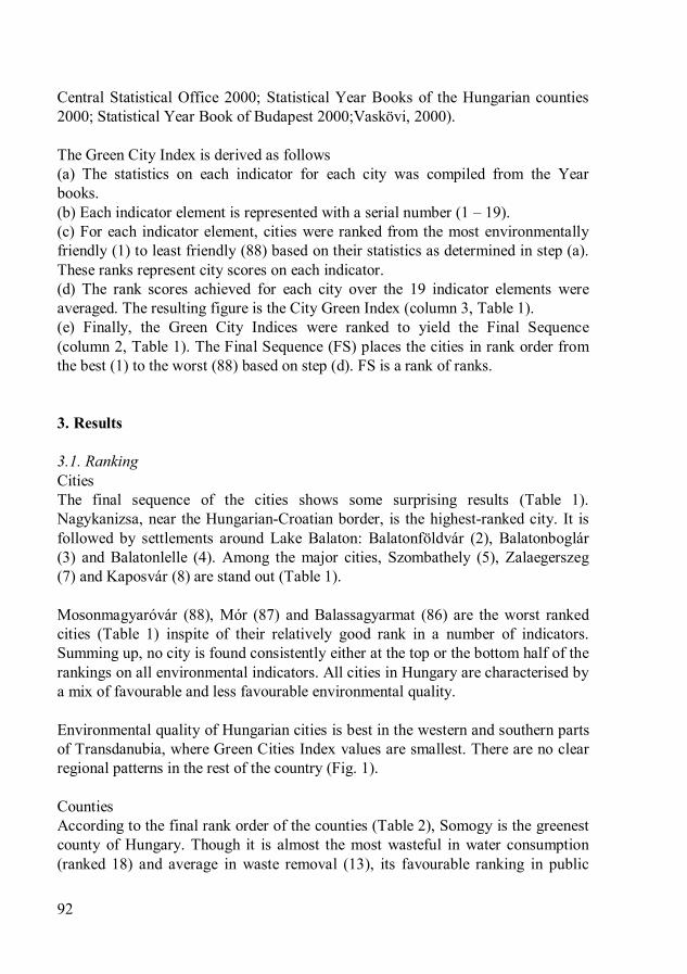
Fig. 1. Environmental quality of cities according to their Green Cities Index High values (circles with large area) = favourable; Low values (circles with small area) = disadvantageous. The numbers indicate the final sequence of the cities (1 = best, 88 = worst). The seven counties, which did the best are all found in Transdanubia (Somogy, Zala, Vas, Komárom-Esztergom, Veszprém, Baranya and Győr-Moson-Sopron), while the five counties, which did the worst, are all found in the Great Hungarian Plain: Szabolcs-Szatmár-Bereg, Hajdú-Bihar, Békés, Bács-Kiskun and Heves. Szabolcs-Szatmár-Bereg, Hajdú-Bihar and Békés; however, do well in some indicators. As in cities, no one county is found consistently at either at the top or the bottom half of the rankings on all indicators. In general, Transdanubian counties enjoy better placement than counties in eastern Hungary (Fig. 2).

94

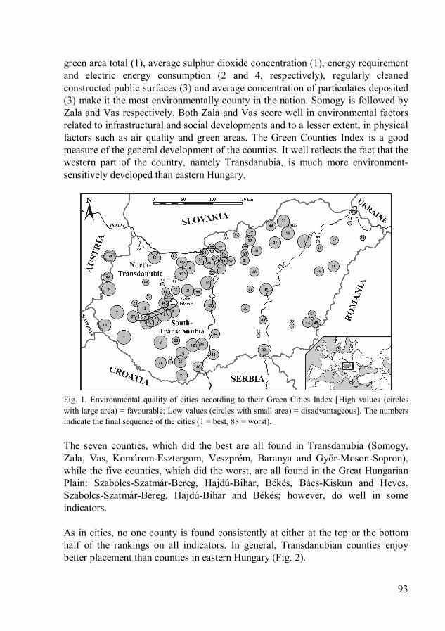
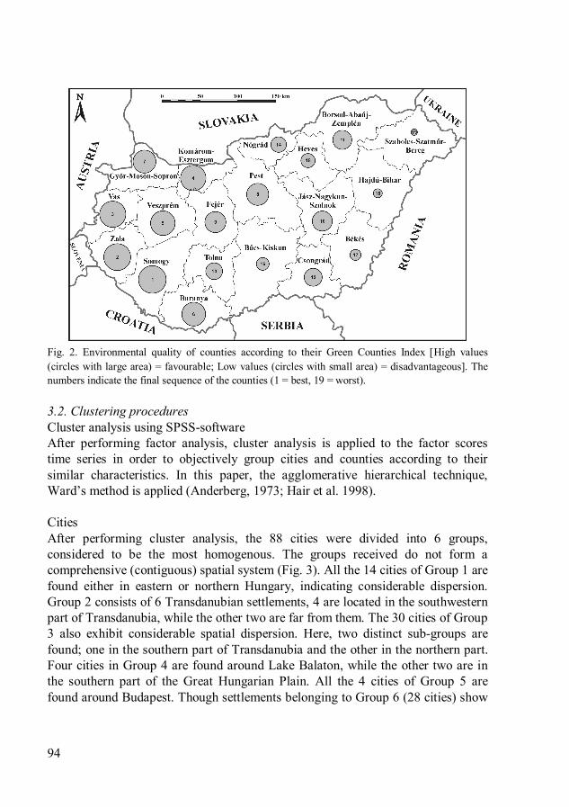
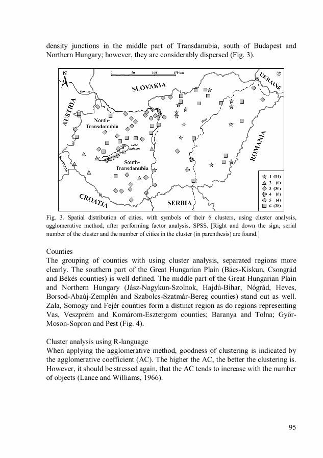
Fig. 2. Environmental quality of counties according to their Green Counties Index High values (circles with large area) = favourable; Low values (circles with small area) = disadvantageous. The numbers indicate the final sequence of the counties (1 = best, 19 = worst). 3.2. Clustering procedures Cluster analysis using SPSS-software After performing factor analysis, cluster analysis is applied to the factor scores time series in order to objectively group cities and counties according to their similar characteristics. In this paper, the agglomerative hierarchical technique, Ward’s method is applied (Anderberg, 1973; Hair et al. 1998). Cities After performing cluster analysis, the 88 cities were divided into 6 groups, considered to be the most homogenous. The groups received do not form a comprehensive (contiguous) spatial system (Fig. 3). All the 14 cities of Group 1 are found either in eastern or northern Hungary, indicating considerable dispersion. Group 2 consists of 6 Transdanubian settlements, 4 are located in the southwestern part of Transdanubia, while the other two are far from them. The 30 cities of Group 3 also exhibit considerable spatial dispersion. Here, two distinct sub-groups are found; one in the southern part of Transdanubia and the other in the northern part. Four cities in Group 4 are found around Lake Balaton, while the other two are in the southern part of the Great Hungarian Plain. All the 4 cities of Group 5 are found around Budapest. Though settlements belonging to Group 6 (28 cities) show

95

density junctions in the middle part of Transdanubia, south of Budapest and Northern Hungary; however, they are considerably dispersed (Fig. 3).

Fig. 3. Spatial distribution of cities, with symbols of their 6 clusters, using cluster analysis, agglomerative method, after performing factor analysis, SPSS. Right and down the sign, serial number of the cluster and the number of cities in the cluster (in parenthesis) are found. Counties The grouping of counties with using cluster analysis, separated regions more clearly. The southern part of the Great Hungarian Plain (Bács-Kiskun, Csongrád and Békés counties) is well defined. The middle part of the Great Hungarian Plain and Northern Hungary (Jász-Nagykun-Szolnok, Hajdú-Bihar, Nógrád, Heves, Borsod-Abaúj-Zemplén and Szabolcs-Szatmár-Bereg counties) stand out as well. Zala, Somogy and Fejér counties form a distinct region as do regions representing Vas, Veszprém and Komárom-Esztergom counties; Baranya and Tolna; Győr-Moson-Sopron and Pest (Fig. 4). Cluster analysis using R-language When applying the agglomerative method, goodness of clustering is indicated by the agglomerative coefficient (AC). The higher the AC, the better the clustering is. However, it should be stressed again, that the AC tends to increase with the number of objects (Lance and Williams, 1966).

96

Table 1. Average of rankings of the environmental indicators considered; namely, the Green Cities Index, and the final sequence of the cities (1 = best, 88 = worst)

City Final sequence

Green Cities Index

City Final sequence

Green Cities Index

City Final sequence

Green Cities Index

Nagykanizsa 1 29.89 Siklós 31 42.26 Esztergom 61 47.74 Balatonföldvár 2 30.58 Szeged 32 42.32 Göd 62 47.78 Balatonboglár 3 30.68 Vác 33 42.47 Dombóvár 63 48.16 Balatonlelle 4 32.11 Dorog 34 42.74 Békés 64 48.37 Szombathely 5 32.89 Debrecen 35 42.84 Lőrinci 65 48.84 Tiszaújváros 6 33.00 Szigetvár 36 42.88 Nagymaros 66 50.00 Zalaegerszeg 7 33.16 Bátonyterenye 37 43.00 Cegléd 67 50.74 Kaposvár 8 33.32 Baja 38 43.26 Hajdúnánás 68 50.84 Siófok 9 34.32 Tata 39 43.32 Pápa 69 51.05 Százhalombatta 10 34.63 Mohács 40 43.95 Szentendre 70 51.14 Fonyód 11 34.74 Gyöngyös 41 44.05 Sümeg 71 51.32 Bonyhád 12 34.79 Békéscsaba 42 44.21 Szécsény 72 51.42 Tapolca 13 35.95 Kőszeg 43 44.37 Komárom 73 51.47 Tatabánya 14 36.26 Ózd 44 44.53 Ajka 74 51.58 Miskolc 15 36.84 Gyula 45 44.63 Pásztó 75 51.63 Komló 16 37.16 Balatonfüred 46 44.79 Mátészalka 76 51.74 Oroszlány 17 37.21 Salgótarján 47 44.89 Budaörs 77 52.00 Lenti 18 37.68 Jászberény 48 45.00 Záhony 78 52.11 Szolnok 19 38.26 Hajdúszobosz

ló 49 16558 Szentlőrinc 79 52.37

Győr 20 38.58 Dunakeszi 50 45.47 Orosháza 80 53.16 Sopron 21 39.05 Hatvan 51 45.63 Kisvárda 81 53.26 Kazincbarcika 22 39.37 Veresegyház 52 46.00 Zirc 82 54.16 Budapest 23 39.74 Balatonalmádi 53 46.21 Kistelek 83 54.26 Székesfehérvár 24 39.89 Kalocsa 54 46.27 Tiszavasvári 84 55.89 Szekszárd 25 39.91 Várpalota 55 46.58 Sajószentpéter 85 56.79 Pécs 26 40.00 Kecskemét 56 46.74 Balassagyarma

t 86 58.05

Keszthely 27 40.32 Nyíregyháza 57 46.95 Mór 87 58.68 Eger 28 40.74 Gárdony 58 47.21 Mosonmagyar

óvár 88 59.21

Dunaújváros 29 41.21 Csongrád 59 47.26 Pilisvörösvár 30 41.63 Veszprém 60 47.42

97

Table 2. Average of rankings of the environmental indicators considered; namely, the Green Counties Index, and the final sequence of the counties (1 = best, 19 = worst; the numbers indicate the counties)

County Final sequence Green Counties Index Somogy 1 6.32 Zala 2 6.79 Vas 3 7.21 Komárom-Esztergom 4 8.79 Veszprém 5 9.26 Baranya 6 9.53 Győr-Moson-Sopron 7 10.00 Pest 8 10.05 Fejér 9 10.16 Jász-Nagykun-Szolnok 10 10.16 Borsod-Abaúj-Zemplén 11 10.42 Csongrád 12 10.47 Tolna 13 10.79 Nógrád 14 11.00 Heves 15 11.21 Bács-Kiskun 16 11.47 Békés 17 11.58 Hajdú-Bihar 18 11.89 Szabolcs-Szatmár-Bereg 19 12.32

Fig. 4. Spatial distribution of counties, with symbols of their 6 clusters, using cluster analysis, agglomerative method, after performing factor analysis, SPSS. Right and down the sign, serial number of the cluster and the number of cities in the cluster (in parenthesis) are found.

98

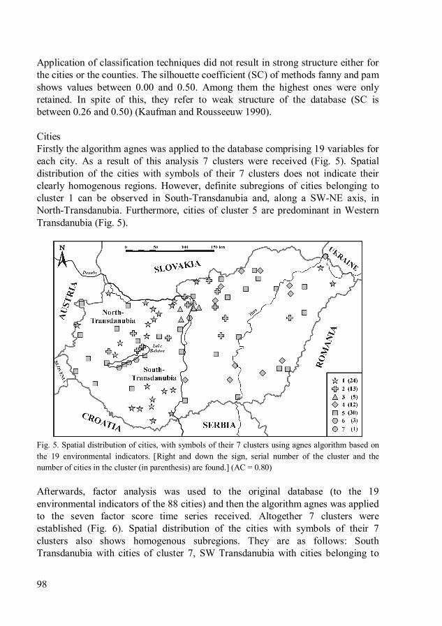
Application of classification techniques did not result in strong structure either for the cities or the counties. The silhouette coefficient (SC) of methods fanny and pam shows values between 0.00 and 0.50. Among them the highest ones were only retained. In spite of this, they refer to weak structure of the database (SC is between 0.26 and 0.50) (Kaufman and Rousseeuw 1990). Cities Firstly the algorithm agnes was applied to the database comprising 19 variables for each city. As a result of this analysis 7 clusters were received (Fig. 5). Spatial distribution of the cities with symbols of their 7 clusters does not indicate their clearly homogenous regions. However, definite subregions of cities belonging to cluster 1 can be observed in South-Transdanubia and, along a SW-NE axis, in North-Transdanubia. Furthermore, cities of cluster 5 are predominant in Western Transdanubia (Fig. 5).

Fig. 5. Spatial distribution of cities, with symbols of their 7 clusters using agnes algorithm based on the 19 environmental indicators. Right and down the sign, serial number of the cluster and the number of cities in the cluster (in parenthesis) are found. (AC = 0.80) Afterwards, factor analysis was used to the original database (to the 19 environmental indicators of the 88 cities) and then the algorithm agnes was applied to the seven factor score time series received. Altogether 7 clusters were established (Fig. 6). Spatial distribution of the cities with symbols of their 7 clusters also shows homogenous subregions. They are as follows: South Transdanubia with cities of cluster 7, SW Transdanubia with cities belonging to

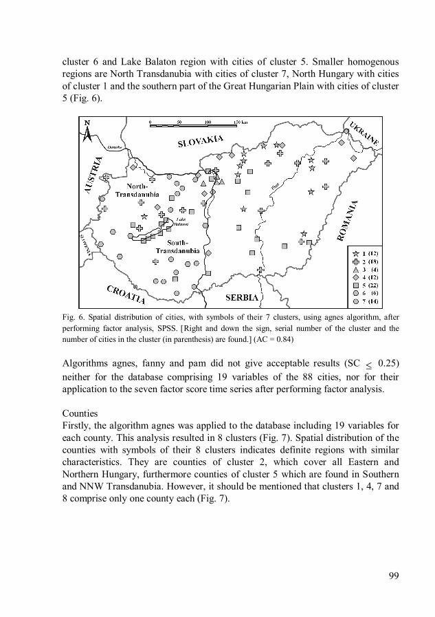
99

cluster 6 and Lake Balaton region with cities of cluster 5. Smaller homogenous regions are North Transdanubia with cities of cluster 7, North Hungary with cities of cluster 1 and the southern part of the Great Hungarian Plain with cities of cluster 5 (Fig. 6).

Fig. 6. Spatial distribution of cities, with symbols of their 7 clusters, using agnes algorithm, after performing factor analysis, SPSS. Right and down the sign, serial number of the cluster and the number of cities in the cluster (in parenthesis) are found. (AC = 0.84) Algorithms agnes, fanny and pam did not give acceptable results (SC 0.25) neither for the database comprising 19 variables of the 88 cities, nor for their application to the seven factor score time series after performing factor analysis. Counties Firstly, the algorithm agnes was applied to the database including 19 variables for each county. This analysis resulted in 8 clusters (Fig. 7). Spatial distribution of the counties with symbols of their 8 clusters indicates definite regions with similar characteristics. They are counties of cluster 2, which cover all Eastern and Northern Hungary, furthermore counties of cluster 5 which are found in Southern and NNW Transdanubia. However, it should be mentioned that clusters 1, 4, 7 and 8 comprise only one county each (Fig. 7).

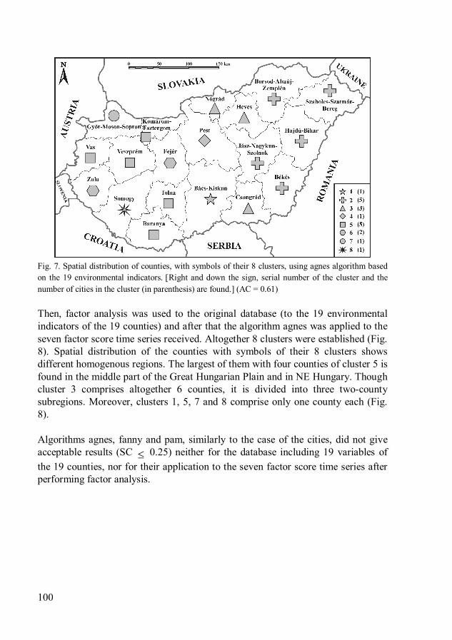
100

Fig. 7. Spatial distribution of counties, with symbols of their 8 clusters, using agnes algorithm based on the 19 environmental indicators. Right and down the sign, serial number of the cluster and the number of cities in the cluster (in parenthesis) are found. (AC = 0.61) Then, factor analysis was used to the original database (to the 19 environmental indicators of the 19 counties) and after that the algorithm agnes was applied to the seven factor score time series received. Altogether 8 clusters were established (Fig. 8). Spatial distribution of the counties with symbols of their 8 clusters shows different homogenous regions. The largest of them with four counties of cluster 5 is found in the middle part of the Great Hungarian Plain and in NE Hungary. Though cluster 3 comprises altogether 6 counties, it is divided into three two-county subregions. Moreover, clusters 1, 5, 7 and 8 comprise only one county each (Fig. 8). Algorithms agnes, fanny and pam, similarly to the case of the cities, did not give acceptable results (SC 0.25) neither for the database including 19 variables of the 19 counties, nor for their application to the seven factor score time series after performing factor analysis.

101

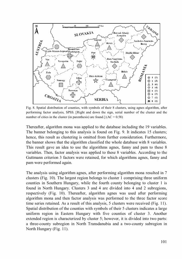
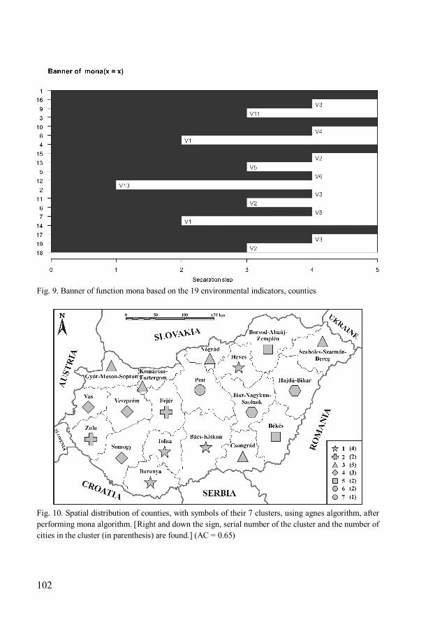
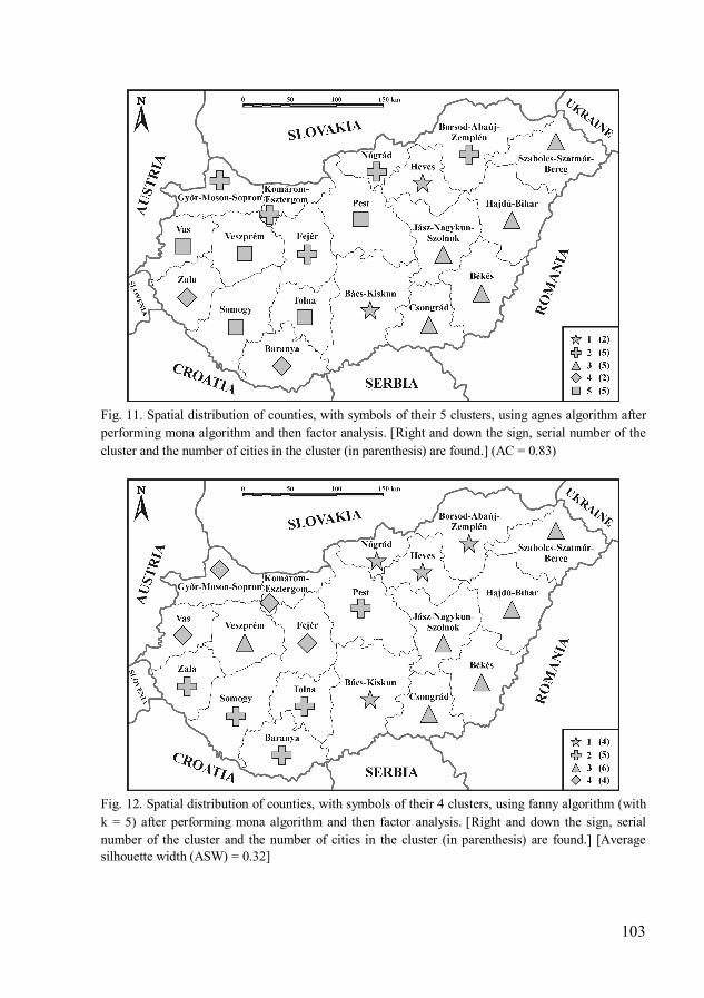
Fig. 8. Spatial distribution of counties, with symbols of their 8 clusters, using agnes algorithm, after performing factor analysis, SPSS. Right and down the sign, serial number of the cluster and the number of cities in the cluster (in parenthesis) are found. (AC = 0.58) Thereafter, algorithm mona was applied to the database including the 19 variables. The banner belonging to this analysis is found on Fig. 9. It indicates 15 clusters; hence, this result as clustering is omitted from further consideration. Furthermore, the banner shows that the algorithm classified the whole database with 8 variables. This result gave an idea to use the algorithms agnes, fanny and pam to these 8 variables. Then, factor analysis was applied to these 8 variables. According to the Guttmann criterion 3 factors were retained, for which algorithms agnes, fanny and pam were performed again. The analysis using algorithm agnes, after performing algorithm mona resulted in 7 clusters (Fig. 10). The largest region belongs to cluster 1 comprising three uniform counties in Southern Hungary, while the fourth county belonging to cluster 1 is found in North Hungary. Clusters 3 and 4 are divided into 4 and 2 subregions, respectively (Fig. 10). Thereafter, algorithm agnes was used after performing algorithm mona and then factor analysis was performed to the three factor score time series retained. As a result of this analysis, 5 clusters were received (Fig. 11). Spatial distribution of the counties with symbols of their 5 clusters indicates a large uniform region in Eastern Hungary with five counties of cluster 3. Another extended region is characterized by cluster 5; however, it is divided into two parts: a three-county subregion in North Transdanubia and a two-county subregion in North Hungary (Fig. 11).

102

Fig. 9. Banner of function mona based on the 19 environmental indicators, counties

Fig. 10. Spatial distribution of counties, with symbols of their 7 clusters, using agnes algorithm, after performing mona algorithm. Right and down the sign, serial number of the cluster and the number of cities in the cluster (in parenthesis) are found. (AC = 0.65)

103

Fig. 11. Spatial distribution of counties, with symbols of their 5 clusters, using agnes algorithm after performing mona algorithm and then factor analysis. Right and down the sign, serial number of the cluster and the number of cities in the cluster (in parenthesis) are found. (AC = 0.83)

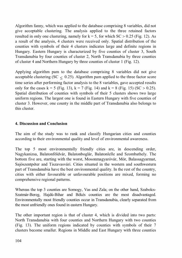
Fig. 12. Spatial distribution of counties, with symbols of their 4 clusters, using fanny algorithm (with k = 5) after performing mona algorithm and then factor analysis. Right and down the sign, serial number of the cluster and the number of cities in the cluster (in parenthesis) are found. [Average silhouette width (ASW) = 0.32]

104

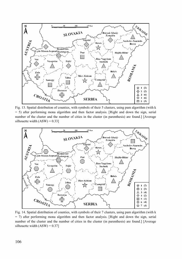
Algorithm fanny, which was applied to the database comprising 8 variables, did not give acceptable clustering. The analysis applied to the three retained factors resulted in only one clustering, namely for k = 5, for which SC 0.25 (Fig. 12). As a result of the analysis, 4 clusters were received only. Spatial distribution of the counties with symbols of their 4 clusters indicates large and definite regions in Hungary. Eastern Hungary is characterized by five counties of cluster 3, South Transdanubia by four counties of cluster 2, North Transdanubia by three counties of cluster 4 and Northern Hungary by three counties of cluster 1 (Fig. 12). Applying algorithm pam to the database comprising 8 variables did not give acceptable clustering (SC 0.25). Algorithm pam applied to the three factor score time series after performing factor analysis to the 8 variables, gave accepted results only for the cases k = 5 (Fig. 13), k = 7 (Fig. 14) and k = 8 (Fig. 15) (SC 0.25). Spatial distribution of counties with symbols of their 5 clusters shows two large uniform regions. The largest one is found in Eastern Hungary with five counties of cluster 3. However, one county in the middle part of Transdanubia also belongs to this cluster. 4. Discussion and Conclusion The aim of the study was to rank and classify Hungarian cities and counties according to their environmental quality and level of environmental awareness. The top 5 most environmentally friendly cities are, in descending order, Nagykanizsa, Balatonföldvár, Balatonboglár, Balatonlelle and Szombathely. The bottom five are, starting with the worst, Mosonmagyaróvár, Mór, Balassagyarmat, Sajószentpéter and Tiszavasvári. Cities situated in the western and southwestern part of Transdanubia have the best environmental quality. In the rest of the country, cities with either favourable or unfavourable positions are mixed, forming no comprehensive regional patterns. Whereas the top 3 counties are Somogy, Vas and Zala; on the other hand, Szabolcs-Szatmár-Bereg, Hajdú-Bihar and Békés counties are the most disadvantaged. Environmentally most friendly counties occur in Transdanubia, clearly separated from the most unfriendly ones found in eastern Hungary. The other important region is that of cluster 4, which is divided into two parts: North Transdanubia with four counties and Northern Hungary with two counties (Fig. 13). The uniform regions indicated by counties with symbols of their 7 clusters become smaller. Regions in Middle and East Hungary with three counties

105

of cluster 3 and North Transdanubia with four counties of cluster 6 are the most characteristic (Fig. 14). Spatial distribution of counties with symbols of their 8 clusters shows smaller uniform regions than that for k = 7. The largest uniform regions are found in Middle and East Hungary with three counties of cluster 3 and in North Transdanubia with also three counties of cluster 6 (Fig. 15). Clustering was performed with cluster analysis using both SPSS software and R-language. Cluster analysis with application of SPSS software resulted in 6 most homogenous groups of cities, which did not form comprehensive spatial patterns. The classification of the counties according to cluster analysis determined also 6 clear groups of them. Cluster analysis using R-language was carried out with different procedures. Algorithms agnes, fanny and pam did not give acceptable results (SC 0.25) neither for the database of the cities, nor for those of the counties. The silhouette coefficient in neither case exceeded the value 0.5, which has been meant that a reasonable structure was found. Clusters received applying algorithm fanny, though having weak structure, indicate large and definite regions in Hungary, which can be circumscribed by clear geographical objects. The agglomerative coefficient (AC), which measures the goodness of the clustering of the dataset, shows highest values when (1) clustering cities with 7 clusters, using algorithm agnes (AC = 0.80; Fig. 5), (2) clustering cities with 7 clusters, using algorithm agnes after performing factor analysis, SPSS (AC = 0.84; Fig. 6) and (3) clustering counties with 5 clusters, using algorithm agnes after performing algorithm mona and then factor analysis (AC = 0.83; Fig. 11).

106

Fig. 13. Spatial distribution of counties, with symbols of their 5 clusters, using pam algorithm (with k = 5) after performing mona algorithm and then factor analysis. Right and down the sign, serial number of the cluster and the number of cities in the cluster (in parenthesis) are found. [Average silhouette width (ASW) = 0.33]

Fig. 14. Spatial distribution of counties, with symbols of their 7 clusters, using pam algorithm (with k = 7) after performing mona algorithm and then factor analysis. Right and down the sign, serial number of the cluster and the number of cities in the cluster (in parenthesis) are found. [Average silhouette width (ASW) = 0.37]

107

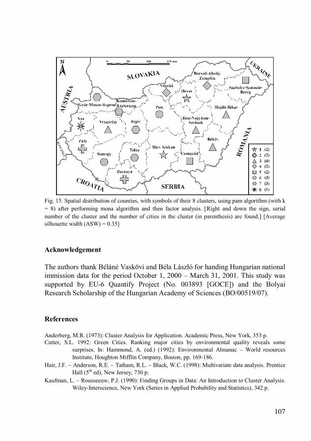
Fig. 15. Spatial distribution of counties, with symbols of their 8 clusters, using pam algorithm (with k = 8) after performing mona algorithm and then factor analysis. Right and down the sign, serial number of the cluster and the number of cities in the cluster (in parenthesis) are found. [Average silhouette width (ASW) = 0.35] Acknowledgement The authors thank Béláné Vaskövi and Béla László for handing Hungarian national immission data for the period October 1, 2000 – March 31, 2001. This study was supported by EU-6 Quantify Project (No. 003893 [GOCE]) and the Bolyai Research Scholarship of the Hungarian Academy of Sciences (BO/00519/07). References Anderberg, M.R. (1973): Cluster Analysis for Application. Academic Press, New York, 353 p. Cutter, S.L. 1992: Green Cities. Ranking major cities by environmental quality reveals some

surprises. In: Hammond, A. (ed.) (1992): Environmental Almanac – World resources Institute, Houghton Mifflin Company, Boston, pp. 169-186.

Hair, J.F. Anderson, R.E. Tatham, R.L. Black, W.C. (1998): Multivariate data analysis. Prentice Hall (5th ed), New Jersey, 730 p.

Kaufman, L. Rousseeuw, P.J. (1990): Finding Groups in Data: An Introduction to Cluster Analysis. Wiley-Interscience, New York (Series in Applied Probability and Statistics), 342 p.

108

Kerényi, A. (1995): General Environmental Protection. Global concerns, possible solutions. Mozaik Educational Studio, Szeged, 383 p. (In Hungarian)

Lance, G.N. Williams, W.T. (1966): A general theory of classificatory sorting strategies: 1. Hierarchical systems. Computer Journal 11: 195.

Vaskövi, B. (2000): National air quality (immission) data 2000. April - September, non-heating half-year. Egészségtudomány 44 (4): 366-377. (in Hungarian)

Publications of the Central Statistical Office, Budapest, Hungary (in Hungarian) Statistical Year Books of the Hungarian counties 2000 (in Hungarian) Statistical Year Book of Budapest 2000 (in Hungarian)