Embed Size (px)
Citation preview

i
The University of Western Australia
School of Electrical, Electronic and Computer Engineering
Environmental Mapping and Software Architecture of
an Autonomous SAE Electric Race Car
Samuel Evans-Thomson
20490234
Supervisor: Professor Dr. Thomas Bräunl
Submitted: 29th October 2017
Word Count: 7959

i
Abstract
This dissertation covers the author’s work on the development of the control system,
software architecture, environmental mapping and visualisation system of an
Autonomous Electric SAE car at the University of Western Australia.
The UWA REV Autonomous SAE Electric Race Car Project is a platform for students
to explore and develop modern electronics and automation systems, and spans
multiple disciplines including electronics, power systems, software design, and
computer science. This year the project team has been working to extend the
autonomous driving functionality of the Electric SAE Race car to be suited to the racing
conditions set by Formula Student Germany. This extension involves implementing
the ability to autonomously drive through a track delineated by traffic cones. On top
of this the team has aimed to improve the platform to facilitate the ease of future
developments in part through the author’s work in building a modularised software
system with the intention of replacing the previous system.
The design considerations, implementation processes and test results of this work is
discussed.

ii
Acknowledgements
I would like to thank the following people for their help during this project:
Prof. Thomas Bräunl for his time, advice and commitment to the project.
The Project Team for their hard work and willingness to help.
Roman Podolski for his extensive help and teaching me to be a better software developer.
Thomas Drage for his knowledge, guidance and support.
My friends and family for providing me with support over the course of the year.

iii
Nomenclature
SAE Society of Automotive Engineers
REV Project Renewable Energy Vehicles Project
UWA University of Western Australia
LiDAR Light Detection And Ranging
LiDAR: Raw Data The series of 3D data points provided by the LiDAR that denote the position of light reflective material in the LiDAR’s field of view.
LiDAR: Object Data The data provided by the LiDAR that denotes the position, size and classification of objects as interpreted by the LiDAR’s internal data processing.
IMU
Inertial Measurement Unit
GPS Global Positioning System
PID Controller Proportional-Integral-Derivative Controller
ASIO Asynchronous Input/Output
Protobuf Google Protocol Buffers Tool
SLAM Simultaneous Localisation and Navigation
FSG Formula Student Germany
FSD Formula Student Driverless ANN Artificial Neural Network

iv
Contents Abstract ................................................................................................................................................ i
Acknowledgements ........................................................................................................................ ii
Nomenclature .................................................................................................................................. iii
1 Introduction .............................................................................................................................. 1
1.1 Motivation .......................................................................................................................... 2
1.2 Goal ....................................................................................................................................... 2
2 Literature Review.................................................................................................................... 3
2.1 Control Systems and Software Design .................................................................... 3
2.1.1 Control ......................................................................................................................... 3
2.1.2 Software Architecture ........................................................................................... 3
2.2 Environmental Mapping .............................................................................................. 4
2.2.1 Navigation Accuracy .............................................................................................. 4
2.2.2 Map Accuracy ............................................................................................................ 4
3 Control System Design .......................................................................................................... 5
3.1 Requirements ................................................................................................................... 5
3.1.1 Navigation .................................................................................................................. 5
3.1.2 Obstacle Avoidance................................................................................................. 5
3.1.3 Safety ............................................................................................................................ 6
3.2 System Capabilities ........................................................................................................ 6
3.2.1 Existing Features ..................................................................................................... 6
3.2.2 Features in Development by Others ................................................................ 7
3.3 Design Considerations .................................................................................................. 8
3.4 Design Process ................................................................................................................. 9
3.5 System Design ................................................................................................................. 10
4 Software Structure ............................................................................................................... 12
4.1 Design Considerations ................................................................................................ 12
4.2 Design Process ............................................................................................................... 13
4.3 Software Design ............................................................................................................. 13
5 Simulation and Visualisation ........................................................................................... 16
5.1 Design Considerations ................................................................................................ 16
5.2 Design Process ............................................................................................................... 16
5.3 Simulation ........................................................................................................................ 16
6 Object Detection .................................................................................................................... 17
6.1 Data Acquisition with Boost::ASIO ........................................................................ 17
6.2 Serialisation with Protobuf ....................................................................................... 17

v
7 Mapping .................................................................................................................................... 18
7.1 Design Process ............................................................................................................... 18
7.2 System Design ................................................................................................................. 18
7.3 Parameter Tuning ......................................................................................................... 20
7.4 Results ............................................................................................................................... 21
8 Conclusion ............................................................................................................................... 22
9 Future Work ............................................................................................................................ 22
References ........................................................................................................................................ 23

1
1 Introduction
Autonomous navigation in automotive vehicles has the potential to significantly increase the
safety and energy efficiency whilst reducing transit times. Designing a car to consistently drive
safely in various contexts such as public roads poses many challenges including sensor fusion,
data analysis, sophisticated control algorithms and reliable safety systems. Beginning in 2009
The Autonomous SAE Car project at the University of Western Australia, led by Prof. Dr.
Thomas Bräunl has developed a drive-by-wire, electric SAE car with autonomous capabilities
with the goal of expanding its abilities to include race track navigation and urban driving. In
2013 considerable progress was made by Drage who developed the safety systems, controllers,
road-edge detection and navigation systems capable of autonomously driving through
recorded GPS waypoints [1]. The path planning was improved by French [2] in 2014 and again
in 2015 by Churack [3] along with improvements to the road-edge detection.
Figure 1: The Autonomous SAE Electric Race Car.

2
1.1 Motivation
The development of an autonomous vehicle provides a platform for the study of robotics,
control systems, sensor integration, data analysis, software engineering, and automotive
electrical hardware design. On top of this the task of developing a driverless race-car provides
a challenge as safety considerations in both hardware and system control must be prioritised
whilst maintaining a goal of high performance.
1.2 Goal
In 2017 Formula Student Germany [4] announced the inclusion of a new competition;
Formula Student Driverless. FSD is an international student-based competition to judge the
performance, engineering practise and design of driverless cars based in Hockenheim,
Germany. The intention of the REV Autonomous Electric SAE Car Team was to make progress
towards preparing the car for the requirements [5] of the FSD competition in coming years as
it is expected that these specifications would become an international standard for driverless
competition. Particular focus was placed on navigation which would involve developing the
navigation system to include cone detection as the FSD track is a cone-delineated circuit as
seen in Figure 2.
Figure 2: Diagram of the cone-delineated track parameters in the FSD specification book. Source: [5]
This dissertation outlines the author’s work in designing an updated control system and
corresponding software architecture, and mapping algorithm suited for cone detection. The
author discusses the benefits of the design, the results of the implementation of the mapping
system and potential future improvements arising from this work.

3
2 Literature Review
Autonomous driving has been an increasingly popular area of research over the last 30 years
as the field grows and more applications for autonomous vehicles are being explored and
implemented. Autonomous cars utilise a combination of control systems, sensors, actuators,
and computer algorithms in a closed-loop controller to achieve various goals including
exploration [6] [7] [8], speed [9], and safety [10]. Relevant literature in the control systems,
software architecture and environmental mapping of autonomous vehicles is discussed below.
2.1 Control Systems and Software Design
The control pipeline of autonomous systems are often coupled to the software architecture as
the control design decisions effect the software implementation. The 2005 DARPA Grand
Challenge; a competition set by DARPA judging the speed with which autonomous vehicles
could navigate a 142 mile long off-road track, was won by ‘Stanley’ an autonomous vehicle
whose development was led by Stanford University [11] and represented a major step forward
in the field of driverless cars.
2.1.1 Control
The control structure used an extension of the Three Layer Architecture discussed in [12]. This
architecture details the use of three layers of control:
Reactive A low-level control layer responsible for effecting changes based on a rapid
feedback loop. Example; a PID controller taking wheel speed inputs used to
maintain vehicle velocity.
Executive Responsible for providing instructions to the reactive layer based on
commands given from the deliberation layer. The processes controlled by the
executive layer usually have fast loop speeds (~1 s) and may include sensor
interpretation and mapping.
Deliberation Responsible for high level problem solving and solution generation such as
calculating an optimal path around a race circuit based on the given map. This
process usually has high computation times therefore updates infrequently.
The team behind Stanley [10] implemented an extension of the Three Layer Control system.
The system architecture was divided roughly into six categories; Sensor Interfaces, Perception,
Planning and Control, User Interfaces, Vehicles Interfaces, and Global Services. Sensor
Interfacing and Perception were responsible for constructing relevant data abstractions from
the sensors and belong to the Executive Layer. Planning and Control derives driving
instructions and path planning from the Perception classes and are categorised as the
Deliberation Layer. The Vehicle Interface systems are responsible for receiving the high level
instructions from the controller and realising these goals by employing a rapid feedback
control loop to govern the actuator outputs.
2.1.2 Software Architecture
The Stanley development team took inspiration from the 2004 winners and adopted the
following philosophy: ‘Treat autonomous navigation as a software problem’ [10, p.66] To
realise the desired control scheme in software the design team implemented a completely real-
time, multithreaded system where each module runs separately of all others and all data
transmission is done globally using timestamped data. This reduces the blocking of software
processes as each individual system will continually run without stopping to wait for other
processes to supply data. The timestamped nature of the data allows real-time control to be

4
applied and the guarantee that the data flow from sensors to actuators will be achieved with
no repeated data.
To ease the software development and testing process the system was built in a modular way
where subsections of the code could be run alone. Also, all data was logged and could be
replayed through the control pipeline using a specifically developed replay module.
Visualisation systems were developed to provide feedback on the systems state in both run
time and simulation modes.
2.2 Environmental Mapping
The ability of autonomous robots to map their environment is another rapidly expanding area
of research with the development of rescue robots [14] and other exploration based
autonomous systems. The detail and speed of robotic mapping is dependent on the desired
detail and intended navigation style.
2.2.1 Navigation Accuracy
For the purposes of navigation based autonomous vehicles it is often the case that low detail
mapping is accurate enough for the path-planner and controllers to operate successfully.
H. Weigel et al. discuss the use of camera and LiDAR sensor fusing to deduct lane positions
and track physical objects [13]. An internal list of detected objects is stored as the car moves.
Objects detected by the LiDAR are compared with the existing objects in the internal map,
unmatched objects are added as new objects while matched objects are fused together and the
internal map is updated. The Mapper removes objects that are outside the observable area of
the vehicle as they are no longer relevant for path planning. Objects that have not been
matched in some time are also removed to reduce the impact of false positive object
identification.
Figure 3: The object detection and integration algorithm. Source: [13]
2.2.2 Map Accuracy
Mapping using Simultaneous Localisation and Mapping has been employed in many
exploration robots as a way to map environments without requiring odometry. In [6] and [7]
the use of sonar and LiDAR with SLAM algorithms is discussed. In SLAM based systems the
distance information provided by the sensors is used to construct a map of the environment.
The map is used to plan the path of the robot, often towards unexplored areas. With each loop
through the control process the world information is compared with the known system to
localise the robot and expand the map.

5
3 Control System Design
The control system for the Autonomous car is required to navigate the vehicle around a
bitumen circuit delineated by cones. In order to achieve this the car is first driven manually
around the circuit to collect waypoints: intermittent position values of the desired path. When
driving autonomously the control system must continuously interpret the data provided by
the sensors and produce instructions for the motors. The car is a closed-loop control system
using sensor data and the given waypoints as inputs and the cars position as the output.
Figure 4: A simplified overview of the control scheme for the autonomous SAE car.
3.1 Requirements
The control system has three primary requirements:
1. The car must drive without human input around the intended track from start to finish.
2. The car must avoid hitting cones.
3. The car must be safe.
3.1.1 Navigation
As stated above, the car will be manually driven around the circuit prior to the autonomous
lap. Once this is complete there will be no human input to the system and any human input
necessitated by the other requirements (primarily safety) represents a failure to comply with
this requirement. For this reason all primary safety systems and navigation controls must be
designed to work autonomously.
3.1.2 Obstacle Avoidance
The described navigation system is capable of meeting the requirement of avoiding the cones
because it attempts to drive a path defined by a manual drive during which no obstacles will
be hit. However, the navigation system cannot precisely match the manual drive path as errors
in the localisation cause noisy results for both the localisation of the waypoints and the

6
obstacles. For this reason the control system must incorporate a feedback loop to adjust its
control parameters for error mitigation. This feedback loop consists of sensing the current car
position and the position and dimensions of objects in the path of the vehicle.
The system is required to avoid all cones but must also avoid other objects that may be in its
path and potentially moving such as people near the track. This requires that the desired path
be updated regularly enough for reliable avoidance.
3.1.3 Safety
The safe operation of the system is the highest priority in each of the relevant subsystems of
the car. Safety controls have been built into the hardware in both the electrical systems and
the low level controllers. In the context of the control system it must be ensured that the car
will not cause injury to people or damage to equipment. As this is the highest priority
requirement, human intervention systems have been included and the expectation is for the
autonomous instructions to be suitable for handling low magnitude threats, such as driving
over cones, but greater threats will be managed by remotely disabling the control system and
bring the car to a stop.
As the control system is required to avoid hitting any obstacles, the planner must provide
suitable paths, safe driving at speeds that allow the path to be followed with reasonable
accuracy and prioritising stopping over progressing through an object.
3.2 System Capabilities
3.2.1 Existing Features
At the beginning of the project the car was equipped with an integrated control system
previously capable of navigating through GPS waypoints using GPS and IMU fused
localisation. The LiDAR provided raw data used to detect road edges though the existing
controller did not integrate road edge avoidance.
See [2] for a more in-depth overview of the existing systems.
Localisation
The localisation comprised of the fusion of GPS coordinates recorded at 1 Hz with acceleration
and bearing data provided by the IMU. A Kalman Filter [15] had previously been implemented
to improve the accuracy of the position data though the project members were not able to
reproduce this functionality resulting in considerable inaccuracies in the GPS data. Position
discrepancies of up to 5 metres were noted during testing.
The bearing of the vehicle was found by fusing the magnetometer readings from the IMU,
which record angle against the earth’s magnetic field, and the GPS tracking angle found by
comparing subsequent GPS position readings. Due to the inaccuracies in the localisation
system it was recognised that further development would be necessary to navigate through
waypoints with low positional error.

7
Object and Road-Edge Detection
The system was capable of examining the object data from the LiDAR to display object
positions as well as running a road-edge detection algorithm on the raw data. The road-edge
detection algorithm takes the central data points and those near them and tests whether they
meet flatness criteria. After compensating for the polar coordinate system of the LiDAR
readings the road provides geometrically flat data within a tolerance range so no great changes
in depth should be noted along the width of the road. Starting from the central readings, points
at a wider angle are iteratively tested in a stepwise process where the correlation coefficient
between the given point and the line of best fit to the road is considered at each point. The
road edge is the point at which the correlation coefficient is the highest whilst the slope
condition is still being met as the next point (the road edge) will diverge from the linear fit.
This approach was improved with the implementation of a Kalman Filter which creates a time-
averaged estimate of the road edge-position assisting in the prediction of the current road
edge.
Control Algorithms
The existing control system uses a series of GPS coordinates (waypoints) to define the goal
positions of the car. Waypoints are removed when the car comes within 2.5 metres of them at
which point the next three waypoints are used to generate the intended movement of the car.
Heading
The steering control algorithm generates a cubic spline as the base-frame using the next three
waypoints. A proportional controller is used to control the steering angle using the bearing
from the GPS and IMU as discussed above to deduce the angle error.
Speed
The speed is controlled using two PID controllers, one for control of the brake and the other
for control of the throttle. The desired speed is produced by assessing the intended turning
angle of the base-frame with two options for desired speed being available based on whether
the turning angle is above or below a given angle.
3.2.2 Features in Development by Others
The project team consists of 8 students with varying levels of involvement and responsibility.
During the year features were assigned to students to develop in parallel with the author’s
work.
Odometry
To improve the localisation of the vehicle wheel speed sensors are being developed to provide
high frequency odometry. Hall Effect sensors are used on the front two wheels to detect pulses
caused by the motion of magnets attached to the wheels. These pulses are counted and recent
measurements are averaged over time to provide current wheel speeds. The rear wheels are
treated similarly though the pulses are provided by the encoders inside the motors. The
steering angle is measured by reading the encoder output of the steering motor.
8
The intention of the odometry project is to provide a live, accurate approximation of the
position offset and angle offset of the car with respect to its starting position. This estimation
can then be fused with the existing GPS and IMU data to provide a potentially much more
accurate localisation of the vehicle with higher update frequency.
Path Planner
An improved path planner is being developed with integrated object avoidance. A set of
waypoints and a set of objects are provided to the path planner which generates a base-frame;
a curve through the waypoints in the correct order. The manoeuvre generator takes the current
position of the vehicle and generates a series of candidate manoeuvres. These manoeuvres are
checked for collisions with objects and graded for quality. A higher quality manoeuvre may be
defined as a path with lower curvature or higher distance from objects. The best candidate is
selected and a series of car positions is derived from the path.
Vision
Prior to this year the only object detection system was through use of the LiDAR. The LiDAR
is accurate but does not detect features such as object colour which may be useful as the
interior and exterior cones will be different colours. An Artificial Neural Network is being
developed that detects cones using video data from a mounted webcam. The neural network
provides coordinates for cones it detects which can be fused with the LiDAR object data.
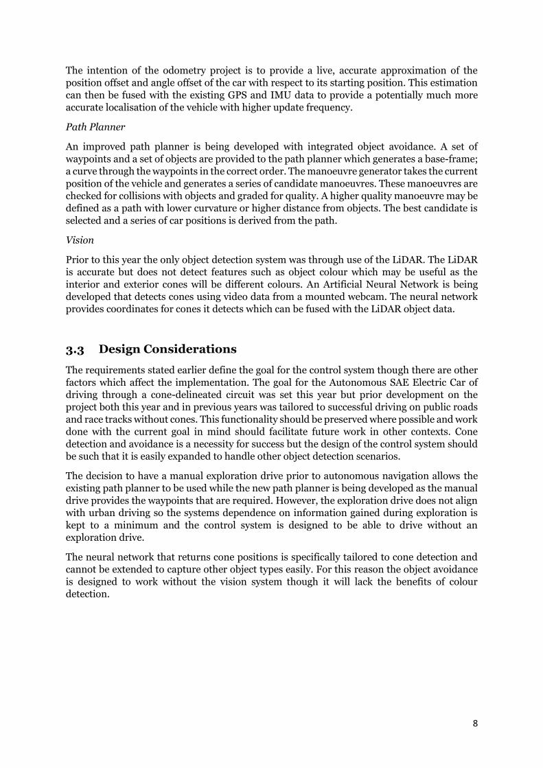
3.3 Design Considerations
The requirements stated earlier define the goal for the control system though there are other
factors which affect the implementation. The goal for the Autonomous SAE Electric Car of
driving through a cone-delineated circuit was set this year but prior development on the
project both this year and in previous years was tailored to successful driving on public roads
and race tracks without cones. This functionality should be preserved where possible and work
done with the current goal in mind should facilitate future work in other contexts. Cone
detection and avoidance is a necessity for success but the design of the control system should
be such that it is easily expanded to handle other object detection scenarios.
The decision to have a manual exploration drive prior to autonomous navigation allows the
existing path planner to be used while the new path planner is being developed as the manual
drive provides the waypoints that are required. However, the exploration drive does not align
with urban driving so the systems dependence on information gained during exploration is
kept to a minimum and the control system is designed to be able to drive without an
exploration drive.
The neural network that returns cone positions is specifically tailored to cone detection and
cannot be extended to capture other object types easily. For this reason the object avoidance
is designed to work without the vision system though it will lack the benefits of colour
detection.

9
3.4 Design Process
After assessing the existing capabilities of the vehicle the following four control schemes were
considered before beginning development:
Control Scheme 1: GPS waypoints are used to dictate the path of the car with live
object detection used for object avoidance. The manoeuvre
generator receives only the objects currently detected.
Control Scheme 2: GPS waypoints are used to dictate the path while object
detection is achieved through application of the mapper which
provides information of all objects in the system.
Control Scheme 3: Waypoints are created by assessing the object positions and
planning a path through them. Object avoidance is inherently
achieved through the waypoint generation.
Control Scheme 4: Localisation is achieved through object detection removing the
dependency on the localisation sensors. The path is generated
the same as Control Scheme 3.
Control Scheme 4 was ruled out early on as the urban driving requirements of the car did not
align with a SLAM system and as development of the odometry systems was already underway.
Control Scheme 1 was also ruled out as it had less potential for speed around the circuit and
limited future improvements. Development began with Control Schemes 2 and 3 still in
discussion; each uses a persistent mapper though Control Scheme 3 requires more
sophisticated object analysis to detect left/right classifications of the objects.
At the time of writing the subsystems required to implement Control Scheme 2 have been
completed and will be integrated together over the next few weeks for system testing. The
inclusion of object-based waypoints has been rejected as accurate localisation is a pre-
requisite for both mapping and GPS waypoint generation so the benefits over using GPS
waypoints for path-planning are minimal.

10
3.5 System Design
At the start of the exploration drive the angle and position of the car are recorded and used to
define the origin. The car is then driven around the circuit storing regular position waypoints
and positional data about the cones. A Baseframe is generated from the waypoints that
encodes directional information for the manoeuvre generator and an initial manoeuvre is
generated.
Figure 5: The control loop used when in autonomous drive mode of the SAE vehicle.

11
Localisation
The Odometer requests the data listed in Table 1
Position Velocity Acceleration Bearing
Wheel Speed Sensors Yes
Steering Angle Sensor Yes
IMU Yes Yes
GPS Yes
Table 1: Localisation Sensors and the corresponding System Input Data
The data is fused to produce a current offset (x,y) pair and bearing with reference to the
starting point of the cars exploration drive.
Object Mapping
The LiDAR object data and the object data from the Vision Neural Network is read in by the
Mapper. All object data is transformed from the cars reference frame to the reference frame
of the origin. The new object information is compared to the existing object data and used to
improve the accuracy of the object localisation.
Path Planner
The object data and car’s position are sent to the Path Planner which generates a collection of
potential manoeuvres. These manoeuvres are filtered for collisions and paths not traversable
by the vehicle and rated based on curvature criteria. The manoeuvre is discretised into a
desired future configuration which is stored.
Controller
The control requests the desired position from the Path Planner and using PID controllers for
the acceleration and braking, and a P controller to dictate the steering angle. These
instructions are sent to the motor controllers which apply the electrical power.
This control loop is repeated until the vehicle reaches the end of the Path Planner Baseframe.

12
4 Software Structure
At the beginning of the project the software was run on a Raspberry Pi 3 with a Linux operating
system. To facilitate the inclusion of computer vision, which requires higher processing
speeds, this was replaced with an NVidia Jetson TX1 computer specifically design with parallel
processing in mind. The existing software had not been designed in a manner that facilitated
the introduction of new features and proved difficult to make design changes so a new software
structure was designed with the intention of porting the existing functionality into it.
The software restructure process did not include re-writing the code responsible for the
functionality; instead, it was the reorganisation of existing functionality into a new system
framework that facilitated error detection, replacement of sub-systems and implementation
of new features.
4.1 Design Considerations
The existing software was built to perform the intended functionality with limited
consideration for software design and suffered from lack of management as the code-base was
passed on to subsequent teams. This rapid prototyping development style is appropriate for
producing functionality quickly but becomes problematic as the functionality grows, a
problem further exacerbated when the members who understand the existing system no
longer maintain it. The new structure was designed with the following considerations.
4.1.1 Separated Data Acquisition and Processing
Data acquisition and data processing are handled by separate systems. The data acquisition
classes are an interface between the hardware and software and provide access to the most
recent unaltered data on request. This allows the timing of data collection to be handled by the
main program loop without introducing disruptions to the process as it waits for new data.
Also, if the hardware is replaced, the only class that needs altering is the data acquisition class
as it is decoupled from any processes that use the data.
Testing new features on the car is not always possible as software development may occur in
times of non-operation of the vehicle. For this reason it is important to be able to simulate the
processes of the car. By decoupling the data collection to other processes the raw data can be
recorded and replayed during simulation to test additional functionality. Recording raw data
as opposed to filtered data allows testing of the filters themselves.
4.1.2 Modularity
The Autonomous SAE Electric Race Car project is continued over multiple years with new
developers joining and leaving the project often. Each developer typically touches on all parts
of the system though the majority of their individual work will be focussed on the improvement
or replacement of a single subsystem. This development behaviour is reliant on students being
able to make changes to or replacements of a subsystem without compromising the others. To
achieve this the software architecture must be modular: It must have individual functions
contained to well defined sub-sections of the code-base. This structure encourages reduced
dependencies between functions and the limitation of influence one section has over any other.

13
4.1.3 Simplicity
Many of the developers are not experts in software engineering or computer science and while
the expectation is that students learn from their work incorporating tools with steep learning
curves will ultimately reduce progress on the project over time as each new developer will need
to spend more time learning the system instead of developing. Any tools incorporated in the
system need to be justified with this in mind.
4.2 Design Process
A new copy of the existing software was created to develop the intended software structure
whilst allowing further work on the existing system. Initially, an attempt was made to
restructure the software by extracting subsystems into new structures whilst maintaining the
ability for the code to be built and run. The road-edge detection was extracted and the new
LiDAR reader was created, though this process exposed the high difficulty of altering the code
structure.
An assessment of the viability of this restructuring method was made and it was decided to do
a bottom-up approach: build the framework skeleton first and insert the existing functionality
into the premade class structures. This approach allowed a clean design slate with far fewer
limitations as the software architecture could be completely redesigned following sound
software design principles whilst maintaining a runnable version of the code for separate
development.
The first step was constructing a skeleton of the software: creating classes with empty
functions that would define the ownership and inheritance structure, and the ordering of
processes. Next, the LiDAR object detection, filtering, and visualisation were added and tested
followed by the vision object detection system. At the time of writing the software structure is
designed in its entirety though still requires the transplantation of core functionality before
performance testing can commence.
4.3 Software Design
The software system is broken up into different tiers of objects that have restricted access to
only the classes that they own with the exception of a few global utility data structures. This
acts much like a traditional corporate structure; few members exist at the top and have high
level control over the system and dictate the distribution of work by giving commands to
managers of different sectors who in turn distribute it to the lower level workers who specialise
in one job.
Tier 1 - Main
The highest tier their exists only one class, the main class that controls the high level flow of
the program and owns manager objects that handle generalised tasks such as data acquisition,
mapping, and path planning etc. The movement of data at lower levels must go through a
common higher tier node as opposed to being passed directly between low level classes to stop
the coupling of functions. A generalised overview of the top levels can be seen in Figure 6.

14
Figure 6: Class ownership diagram of the Tier 1 and Tier 2 classes.
The main class is responsible for dictating the control flow as discussed in section 3 and the
movement of data between the sub-systems. For example: The Visualiser uses object data
provided by the Mapper, this information is requested by main and passed to the Visualiser as
opposed to the Visualiser directly requesting it from the Mapper. This allows the Mapper to be
altered or replaced without needing any changes to be made to the Visualiser as long as the
data by the new Mapper is provided in the existing format.
Tier 2 – Sensor Manager
The Sensor Manager is responsible for requesting data from the individual sensors who in turn
interface with receiver classes which handle the acquisition of information from the hardware.
The various receivers run in separate threads to the main control process and update local
data variables when new data comes in which guarantees that the Main class always has access
to the latest available data on request.
Figure 7: Sensor Manager class ownership structure.

15
Tier 2 – Mapper and Visualiser
The Mapper receives object information including positions and dimensions of the car,
physical objects and waypoints with reference to the starting position of the car. The most
recent object information is available to the Main class on request. Two data processing classes
are utilised to improve the accuracy of the object information that will be discussed in
Section 6. The Visualiser displays the object data provided by the Mapper and is discussed in
Section 5.
Figure 8: Mapper class ownership
Tier 2 – Path Planner and Controller
The Path Planner receives object data and vehicle position data to produce a series of desired
car positions. A mathematical curve is generated by the Baseframe class which the Maneuver
class uses to generate potential car positions. The Controller is given these desired positions
and outputs instructions to the low level motor controllers. Development of a new controller
is under development so the software structure is not yet well defined.
Figure 9: Path Planner class ownership

16
5 Simulation and Visualisation
To aid in the development of the Mapper, Vision, and Path-Planner a data visualisation and
simulation system was designed and implemented on the Autonomous car and made available
for personal computers.
5.1 Design Considerations
The Vision and LiDAR object detection, and Mapper
output required a visual reference to verify the
correlation between the real word and the sensor’s
interpretations. The visualiser has the following
requirements:
Display the objects provided by the mapper.
Limit the impact on the performance of the
control software.
Be runnable on personal computers.
Run in parallel to the control software.
5.2 Design Process
SDL2 [16] Simple DirectMedia Layer version 2 was
chosen as the graphics platform due to it being
lightweight, performance focussed C++ library;
limiting the impact on the performance of the
software without requiring incorporating a new
programming language to the system.
The viewing window was programmed to run
separately to the control program and can scale to fit
the screen installed on the vehicle or any computers
it is run on.
5.3 Simulation
During the project there were multiple periods during which the car could not be driven due
to hardware upgrades and bug fixes. To decouple the testing of software with the state of the
hardware a basic simulator was developed. The data acquisition systems were designed to
store data in a format that allows them to be replayed through the software. Once the data
acquisition was successfully implemented functions were built to feed the data back through
the software at a scalable rate to enable performance testing.
Figure 10: Object Visualiser window displaying objects detected by the LiDAR
17
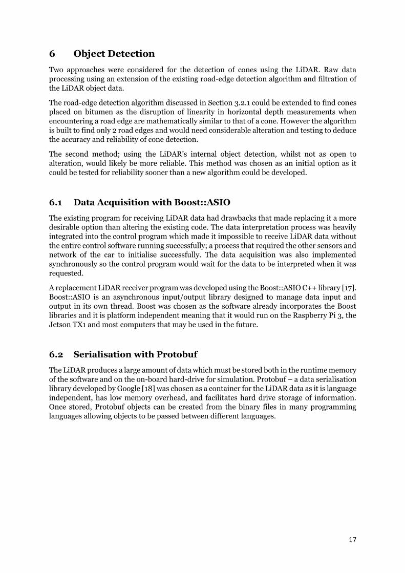
6 Object Detection
Two approaches were considered for the detection of cones using the LiDAR. Raw data
processing using an extension of the existing road-edge detection algorithm and filtration of
the LiDAR object data.
The road-edge detection algorithm discussed in Section 3.2.1 could be extended to find cones
placed on bitumen as the disruption of linearity in horizontal depth measurements when
encountering a road edge are mathematically similar to that of a cone. However the algorithm
is built to find only 2 road edges and would need considerable alteration and testing to deduce
the accuracy and reliability of cone detection.
The second method; using the LiDAR’s internal object detection, whilst not as open to
alteration, would likely be more reliable. This method was chosen as an initial option as it
could be tested for reliability sooner than a new algorithm could be developed.
6.1 Data Acquisition with Boost::ASIO
The existing program for receiving LiDAR data had drawbacks that made replacing it a more
desirable option than altering the existing code. The data interpretation process was heavily
integrated into the control program which made it impossible to receive LiDAR data without
the entire control software running successfully; a process that required the other sensors and
network of the car to initialise successfully. The data acquisition was also implemented
synchronously so the control program would wait for the data to be interpreted when it was
requested.
A replacement LiDAR receiver program was developed using the Boost::ASIO C++ library [17].
Boost::ASIO is an asynchronous input/output library designed to manage data input and
output in its own thread. Boost was chosen as the software already incorporates the Boost
libraries and it is platform independent meaning that it would run on the Raspberry Pi 3, the
Jetson TX1 and most computers that may be used in the future.
6.2 Serialisation with Protobuf
The LiDAR produces a large amount of data which must be stored both in the runtime memory
of the software and on the on-board hard-drive for simulation. Protobuf – a data serialisation
library developed by Google [18] was chosen as a container for the LiDAR data as it is language
independent, has low memory overhead, and facilitates hard drive storage of information.
Once stored, Protobuf objects can be created from the binary files in many programming
languages allowing objects to be passed between different languages.

18
7 Mapping
The object data supplied by the LiDAR are given with positions relative to the car which is
useful for potential collision detection but not for the path planning methods discussed in
Section 3.4.1. The control system requires that an accurate representation of the physical
world and the car’s position within it be available on request. To do this the Mapper class was
created to place objects in an absolute reference frame as well as filtering and improving the
data.
7.1 Design Process
The Mapper stores its best estimate at the world around it which it improves when it receives
new information. This improvement method involves checking each of the new objects with
the existing objects for a ‘match’ and updating the estimate based on the properties of the new
object. Two algorithms were developed to achieve this; an object matching algorithm and a
time smoothing algorithm.
The design for the Mapper began with an assessment of the LiDAR object position detection
accuracy. This was achieved by printing out the object information live as the LiDAR detected
large cones (500 mm) placed at known positions with respect to the car. The position accuracy
of the cones was found to be within 300 mm at distances of less than 50 m which roughly
correlates to the width of the base of the cones.
The ability of the Mapper to correctly match objects is dependent on the accuracy of the LiDAR
and the accuracy of the car localisation. As it was assumed that the car localisation would have
low error (< 1 m) compared to the gaps between cones (3.5 m minimum [5]) the Mapper’s
position tolerance could be increased to 1.75 m without introducing false positives in the
matching algorithm.
As the odometry was not complete at the time of writing the Mapper was not able to be tested
in a live environment. Instead, a session of LiDAR object data was recorded during a drive
between cones and used during simulation. As the odometry of the drive was not available the
session was video recorded and the cars movement was extracted from the video and emulated
in the simulation. The time smoothing parameters were tuned to produce the desired results
which are discussed in Section 5.2.3.
7.2 System Design
Object Localisation
The LiDAR provides Cartesian coordinates of the size and position of objects. The localisation
uses the latest car position and rotation measurements to transform the coordinates to the
absolute reference frame. This is done using the following formulae:

19
𝑑𝑐,𝑐→𝑜 = √𝑦𝑐,𝑜2 + 𝑥𝑐,𝑜
2
𝜃𝑤,𝑐→𝑜 = arctan (𝑥𝑐,𝑜𝑦𝑐,𝑜
) + 𝜃𝑤,𝑐
𝑦𝑤,𝑜 = 𝑑𝑐,𝑜 cos(𝜃𝑤,𝑐→𝑜) + 𝑦𝑤,𝑐
𝑥𝑤,𝑜 = 𝑑𝑐,𝑜 sin(𝜃𝑤,𝑐→𝑜) + 𝑥𝑤,𝑐
Where the first subscript denotes the reference frame and the second denotes the object/s. Note: Angles are measured clockwise from the y-axis.
Figure 11: The object (red) detected by the vehicle (green) in the reference frame of the Mapper (blue).
The green axis is the reference frame of the car.
Object Filtering
The context of the autonomous drive provides clean data as the flat bitumen environment
lacks geometric features other than the cones; however, false positives are still provided by the
LiDAR possibly due to dust or marks on the screen or unavoidable noise due to the scattering
of light. The object filter works towards providing only object information for relevant objects
by rejecting false positives based on distance and size. Objects that are too small or too far
away from the car are deleted to reduce processing time and erroneous path planning.
Time Smoothing
During testing of the cone detection it was found that the detection would be missed
periodically with the cones flickering in and out of detection even when static. Also,
occasionally objects would be briefly detected that had no obvious physical counterpart. Both
sets of behaviour are undesired as the Mapper needs to develop a permanent list of the relevant
objects in the system. To counter this time-sensitive behaviour the Time Smoother was
developed to combine the available data into a more relevant and accurate assessment of the
environment.
Each frame of LiDAR data contains each object the LiDAR is currently detecting. After a frame
is recorded and filtered the objects are stored in the Time Smoother and assigned an age value,
match counter, and a confidence value. For each subsequent frame the detected objects are
compared with the existing objects for matches, an object is considered a match if they have
dimensions and positions within the tolerances seen below.
Position: The positions of two objects are considered a match if the distance between the
two object centres is less than some constant D.
Size: The sizes of two objects are considered a match if the height of the larger object
is less that (1 + Sy) times that of the smaller object and the width of the wider
object is less than (1 + Sx) times that of the narrower object.
20
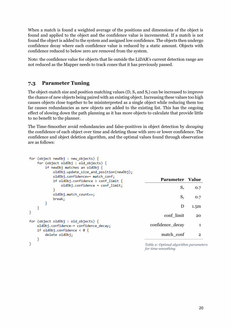
When a match is found a weighted average of the positions and dimensions of the object is
found and applied to the object and the confidence value is incremented. If a match is not
found the object is added to the system and assigned low confidence. The objects then undergo
confidence decay where each confidence value is reduced by a static amount. Objects with
confidence reduced to below zero are removed from the system.
Note: the confidence value for objects that lie outside the LiDAR’s current detection range are
not reduced as the Mapper needs to track cones that it has previously passed.
7.3 Parameter Tuning
The object-match size and position matching values (D, Sx and Sy) can be increased to improve
the chance of new objects being paired with an existing object. Increasing these values too high
causes objects close together to be misinterpreted as a single object while reducing them too
far causes redundancies as new objects are added to the existing list. This has the ongoing
effect of slowing down the path planning as it has more objects to calculate that provide little
to no benefit to the planner.
The Time-Smoother avoid redundancies and false-positives in object detection by decaying
the confidence of each object over time and deleting those with zero or lower confidence. The
confidence and object deletion algorithm, and the optimal values found through observation
are as follows:
Parameter Value
Sx 0.7
Sy 0.7
D 1.5m
conf_limit 20
confidence_decay 1
match_conf 2
Table 2: Optimal algorithm parameters for time-smoothing

21
7.4 Results
The car was driven in a straight line through a lane behind the engineering workshops (seen right) to record data for the simulation. After emulating the odometry as discussed above the Mapper was able to deduce the positions of the cones and map its surroundings with success. The drive provided a total of 464 ‘frames’ of object data. Each frame contains a snapshot of the LiDAR’s observation and can contain any number of objects. Without filtering or Time-smoothing the Mapper presented the results seen in Figure 13. A total of 3580 objects were discovered over the 464 frames. The filtered results (right) provides a similar level of detail with only 84 objects. This shows a massive reduction in redundant information and confirms the viability of the Mapper as an object provider for the path planner.
Figure 12: The testing environment used during the test recording. The corresponding visualiser output
is seen in figure 13.
Figure 13: The Mapper output with no object smoothing or deletion (left) compared to the same data set with object smoothing and deletion (right). The red rectangle is the vehicle’s current position.

22
8 Conclusion
This project demonstrated the successful implementation of an environmental mapper using
LiDAR technology with the capabilities of displaying object data from other sources including
the cone-detecting computer vision system. The mapper is able to detect and store relevant
information from the environment whilst reducing redundancies that would cause
performances losses in a live drive. To enable troubleshooting and aid future development a
standalone, low-overhead visualiser was programmed and installed on the vehicle to display
object data and odometry during both live drives and during simulation on separate systems.
A new control scheme and software system was designed and partially implemented with
considerable focus on the ease of future developments on the vehicle. Using sound software
engineering paradigms the software was built to enable simultaneous development, testing of
subsystems, exchangeability of modules, and expansion of functionality.
9 Future Work
Unfortunately due to the various subsystems being developed in parallel at different rates the
software system was not able to be implemented and tested on the car as new developments
were made on the pre-existing branch to maintain functional progress on the vehicle. This
integration along with testing will be achieved over the following weeks as the team prepares
for demonstration.
Beyond the software integration the visualiser will be extended to display the intended
manoeuvre and Baseframe of the vehicle to expose the decision making of the system to the
observers. The visualisation data will be asynchronously supplied to computers on the network
so that the same image feed can be observed outside the vehicle.
Currently the control and visualisation on board the Jetson TX1 are run in serial with the path-
planner which could be altered so that all three run on separate threads to reduce blocking due
to the processing requirements of each module.

23
References
[1] Thomas H. Drage, “Development of a Navigation Control System for an Autonomous Formula SAE-Electric Race Car”, Final Year Thesis, School of Electrical, Electronic and Computer Engineering, University of Western Australia, WA, 2013.
[2] Martin French, “Advanced Path Planning for an Autonomous SAE Electric Race Car, Final Year Thesis, School of Electrical, Electronic and Computer Engineering, University of Western Australia, WA, 2014.
[3] Thomas Churack, “Improved Road-Edge Detection and Path-Planning for an Autonomous SAE Electric Race Car”, Final Year Thesis, School of Electrical and Electronic Engineering, University of Western Australia, WA, 2015.
[4] Formula Student Germany, website: https://www.formulastudent.de/ accessed: 29/10/2017
[5] FSG DV Technical Specification 2017, available at: https://www.formulastudent.de/fsg/rules/, accessed: 25/10/2017
[6]
D. Trivun, E. Salaka, et al. “Active SLAM-Based Algorithm for Autonomous Exploration with Mobile Robot”, University of Sarajevo, 2015
[7] C. Leung, S. Huang, G. Dissanyake, “Active SLAM in Structure Environments”, Australian Research Council, September 2007
[8] F. Tungadi, L. Kleeman, “Autonomous loop exploration and SLAM with fusion of advanced sonar and laser polar matching”, Intelligent Robotics Research Centre, Department of Electrical and Computer Systems Engineering, Monash University, Australia, April 2011
[9] J. Ni, J. Hu, “Dynamics control of autonomous vehicle at driving limits and experiment on an autonomous formula racing car”, School of Mechanical Engineering, Beijing Institute of Technology, August 2016
[10]
M. Edwards, A. Nathanson, et al., “Assessment of Integrated Pedestrian Protection Systems with Autonomous Emergency Braking (AEB) and Passive Safety Components”, Traffic Injury Prevention, 2015
[11]
Thrun, M. Montemerlo, H. Dahllamp et. al. “Stanley: The Robot That Won the DARPA Grand Challenge” in The 2005 DARPA Grand Challenge, M. Buelher, K. Iagnemma, S. Signh, Eds., Berlin: Springer, 2007, pp. 1-43.
[12]
S. Russel, P. Norvig, “Artificial Intelligence A Modern Approach Third Edition”, Pearson Eduction, Inc. 2010.
[13]
H. Weigel, P. Lindner, G. Wanielik, “Vehicle Tracking with Lane Assignment by Camera and Sensor Fusion” Chemnitz Uniersity of Technology, 2009
[14] Z. Zhang, G. Nejat, “Intelligent Sensing Systems for Rescue Robots: Landmark Identification and Three-Dimensional Mapping or Unknown Cluttered Urban Search and Rescue Environments “, Advanced Robotics 23, February 2009

24
[15] R. E. Kalman, “A New Approach to Linear Filtering and Prediction Problems”, Research Institute for Advanced Study, Baltimore, 1960
[16] Simple DirectMedia Layer Version 2.0, available: https://www.libsdl.org/
[17] Boost ASIO Library,
available: http://www.boost.org/doc/libs/1_65_1/doc/html/boost_asio.html
[18] Google Protocol Buffers – Protobuf, available: https://developers.google.com/protocol-buffers/