ENVIRONMENTAL LAYERS MEETINGIPLANT TUCSON

2012-04-03

RoundupBenoit Parmentier

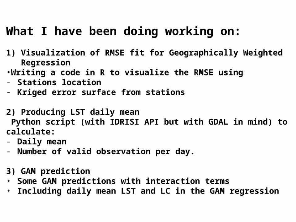
What I have been doing working on:

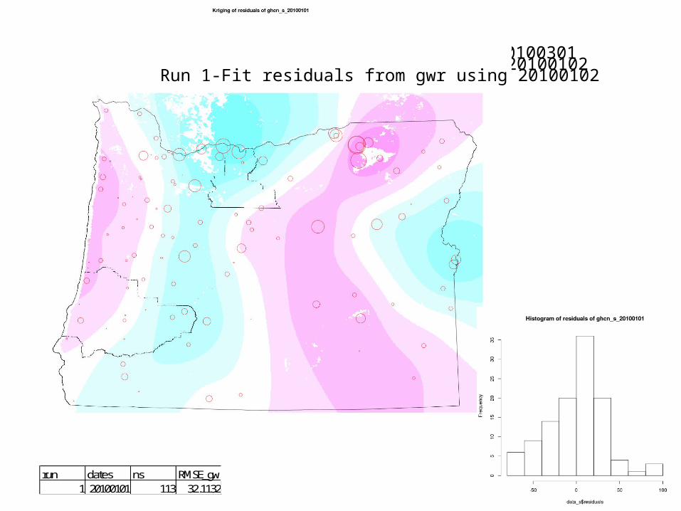
1) Visualization of RMSE fit for Geographically Weighted Regression •Writing a code in R to visualize the RMSE using- Stations location- Kriged error surface from stations

2) Producing LST daily mean Python script (with IDRISI API but with GDAL in mind) to calculate:- Daily mean- Number of valid observation per day.

3) GAM prediction• Some GAM predictions with interaction terms• Including daily mean LST and LC in the GAM regression

1) Visualization of RMSE fit for Geographically Weighted Regression •Writing a code in R to visualize the RMSE using- Stations location- Kriged error surface from stations

1)VISUALIZATION OF RMSE Moving beyond aggregate statistic…

0

5

10

15

20

25

30

35

40

45

RM

SE fi

t (d

eg

C *

10

)

Interpolation Date

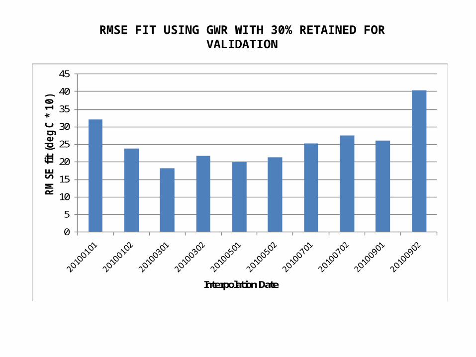
RMSE FIT USING GWR WITH 30% RETAINED FOR VALIDATION

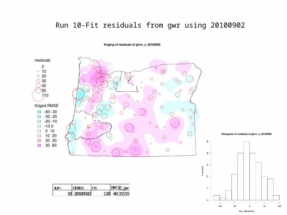
Run 10-Fit residuals from gwr using 20100902

run dates ns RMSE_gwr110 20100902 120 40.31519

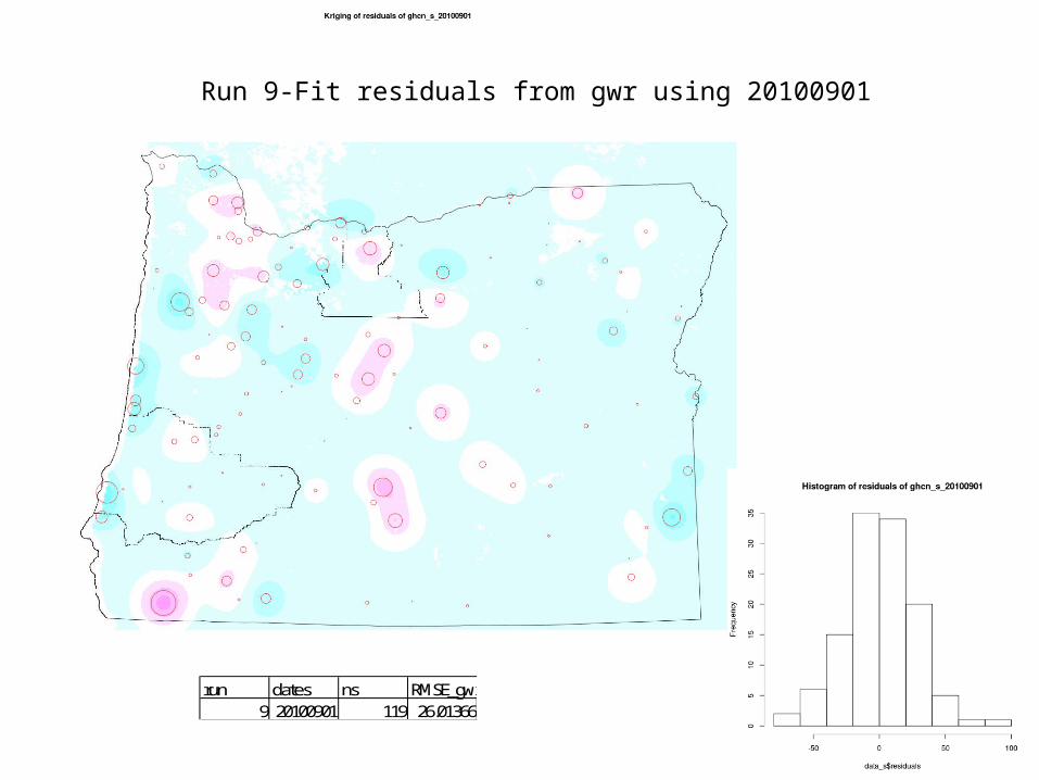
Run 9-Fit residuals from gwr using 20100901

run dates ns RMSE_gwr19 20100901 119 26.01366

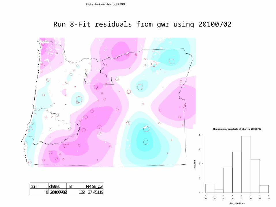
Run 8-Fit residuals from gwr using 20100702

run dates ns RMSE_gwr18 20100702 120 27.45119

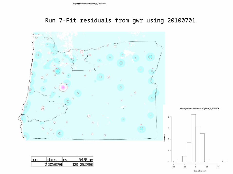
Run 7-Fit residuals from gwr using 20100701

run dates ns RMSE_gwr17 20100701 123 25.27986

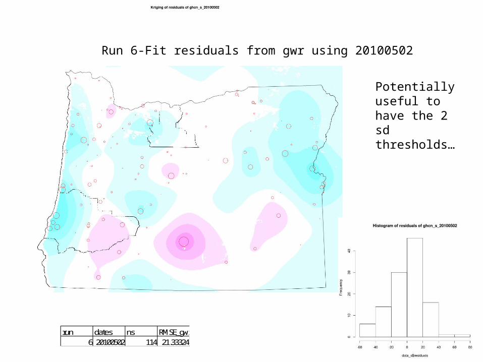
Fit residuals from gwr using 20100701Run 6-Fit residuals from gwr using 20100502

run dates ns RMSE_gwr16 20100502 114 21.33324

Potentially useful to have the 2 sd thresholds…

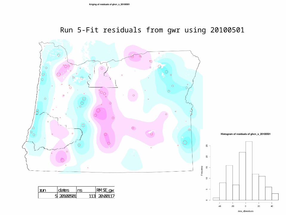
Run 5-Fit residuals from gwr using 20100501

run dates ns RMSE_gwr15 20100501 113 20.00117

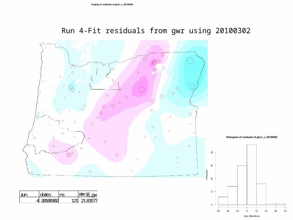
Run 4-Fit residuals from gwr using 20100302

run dates ns RMSE_gwr14 20100302 121 21.83577

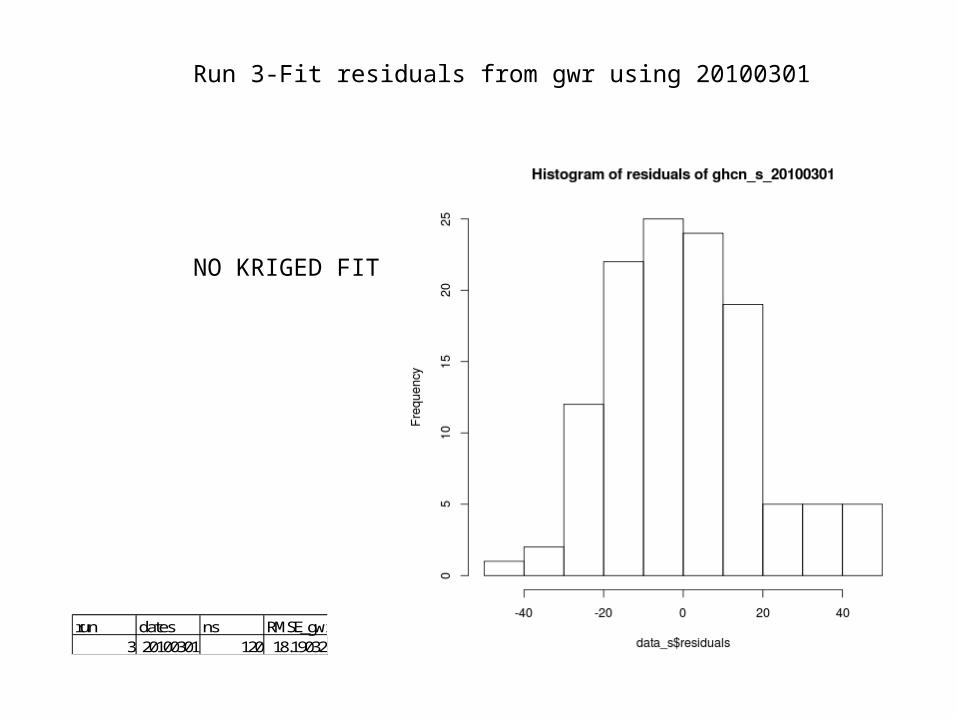
Run 3-Fit residuals from gwr using 20100301

NO KRIGED FIT

run dates ns RMSE_gwr13 20100301 120 18.19032

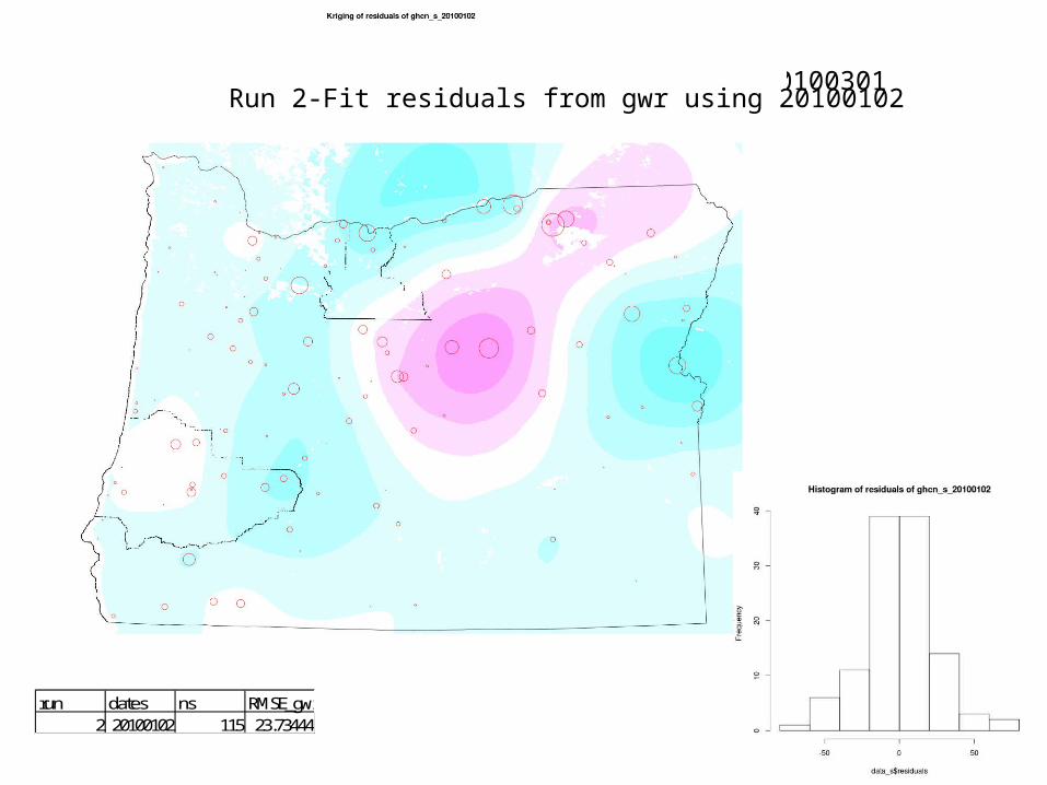
Run 8-Fit residuals from gwr using 20100301Run 2-Fit residuals from gwr using 20100102

run dates ns RMSE_gwr12 20100102 115 23.73444

Run 8-Fit residuals from gwr using 20100301Run 9-Fit residuals from gwr using 20100102

Run 1-Fit residuals from gwr using 20100102

run dates ns RMSE_gwr11 20100101 113 32.1132

•Python script (with IDRISI API but with GDAL in mind) to calculate:- Daily mean- Number of valid observation per day.

LST DAILY MEAM PRODUCTION

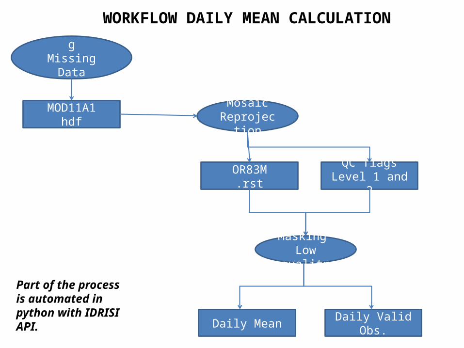
MOD11A1hdf

OR83M.rst

MosaicReprojection

QC flagsLevel 1 and 2

Masking Low quality

Daily Mean Daily Valid Obs.

WORKFLOW DAILY MEAN CALCULATION

Part of the process is automated in python with IDRISI API.

DownloadingMissing Data Assessment

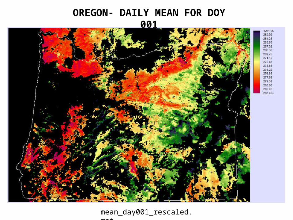
OREGON- DAILY MEAN FOR DOY 001

mean_day001_rescaled.rst

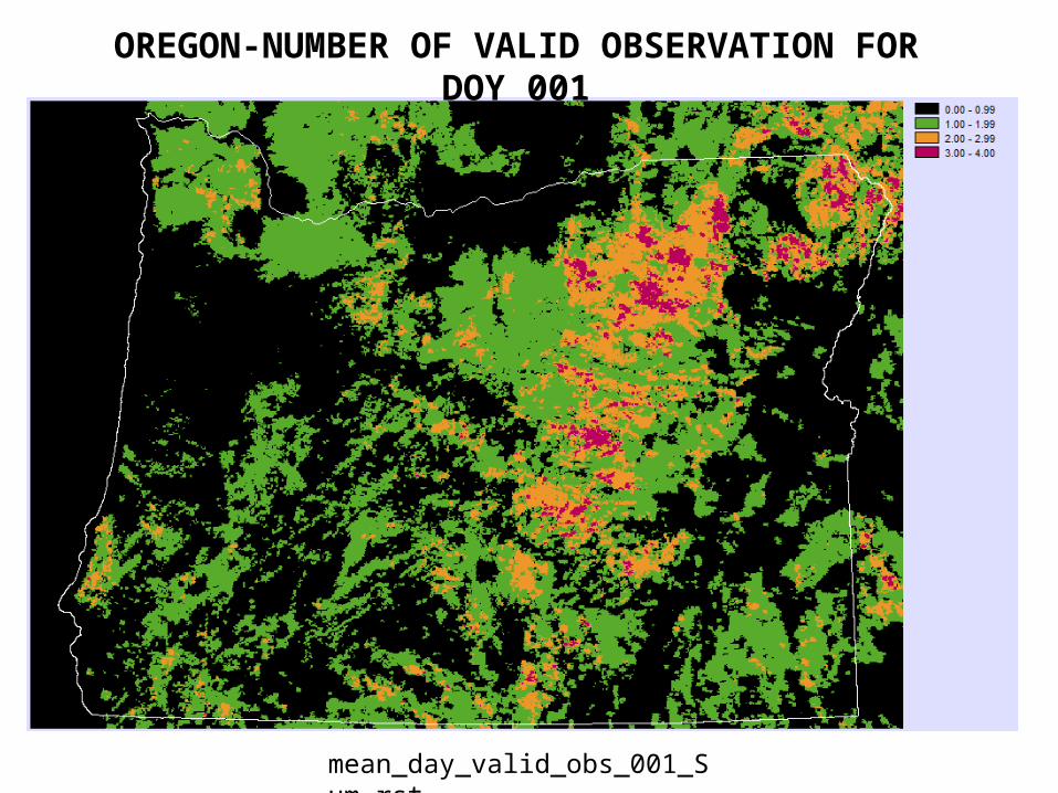
OREGON-NUMBER OF VALID OBSERVATION FOR DOY 001

mean_day_valid_obs_001_Sum.rst

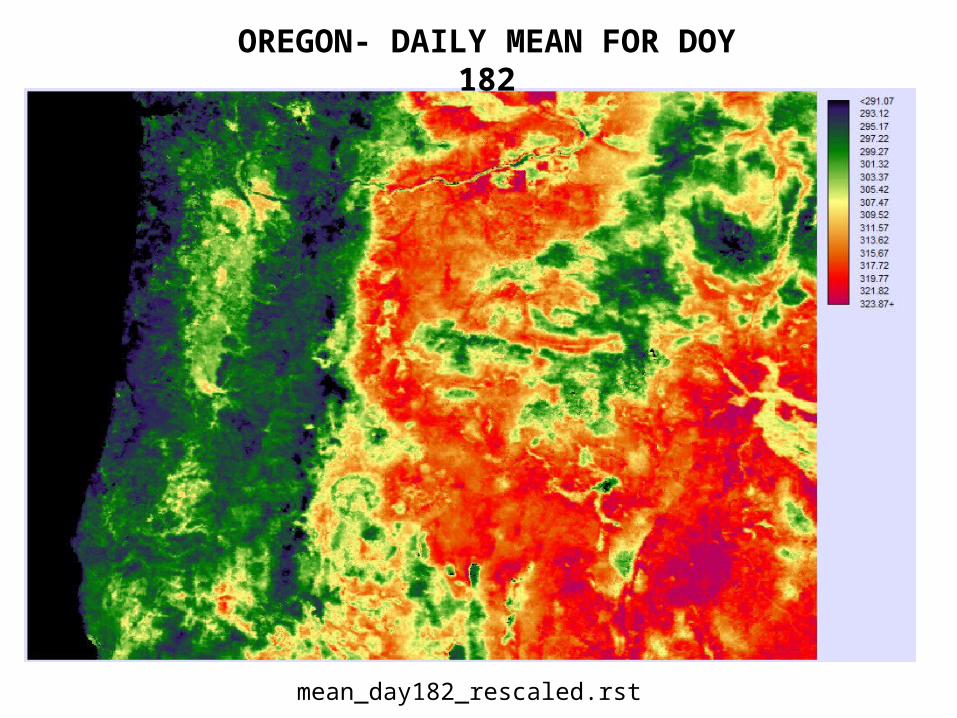
OREGON- DAILY MEAN FOR DOY 182

mean_day182_rescaled.rst

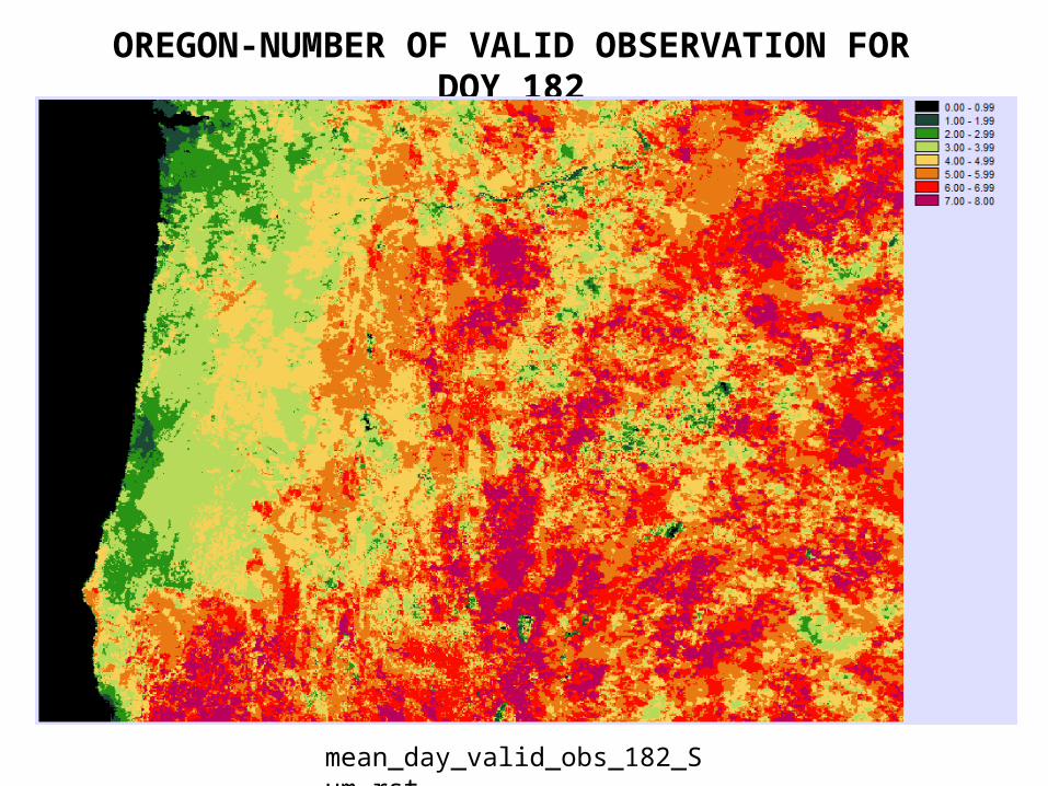
OREGON-NUMBER OF VALID OBSERVATION FOR DOY 182

mean_day_valid_obs_182_Sum.rst

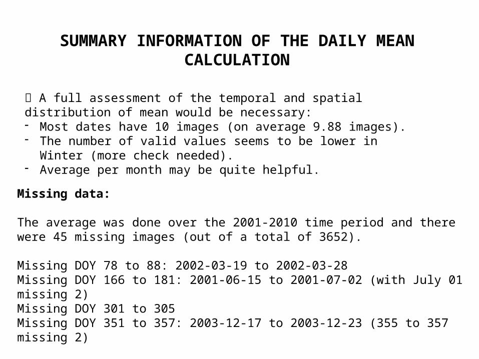
SUMMARY INFORMATION OF THE DAILY MEAN CALCULATION

A full assessment of the temporal and spatial distribution of mean would be necessary:- Most dates have 10 images (on average 9.88 images).- The number of valid values seems to be lower in Winter (more check needed).- Average per month may be quite helpful.

Missing data:

The average was done over the 2001-2010 time period and there were 45 missing images (out of a total of 3652).

Missing DOY 78 to 88: 2002-03-19 to 2002-03-28Missing DOY 166 to 181: 2001-06-15 to 2001-07-02 (with July 01 missing 2)Missing DOY 301 to 305Missing DOY 351 to 357: 2003-12-17 to 2003-12-23 (355 to 357 missing 2)

3)GAM MODELING USING LST AND LC

GAM regressions:• Some GAM predictions with interaction terms• Including daily mean LST and LC in the GAM regression

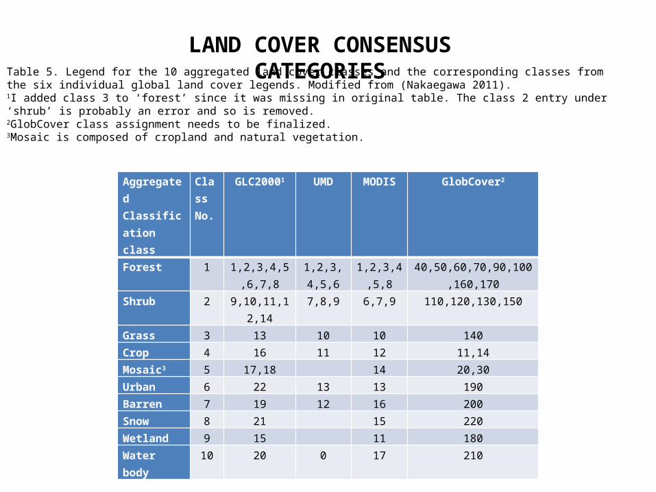
AggregatedClassification class

Class No.

GLC20001 UMD MODIS GlobCover2

Forest 1 1,2,3,4,5,6,7,8

1,2,3,4,5,6

1,2,3,4,5,8

40,50,60,70,90,100,160,170

Shrub 2 9,10,11,12,14 7,8,9 6,7,9 110,120,130,150Grass 3 13 10 10 140Crop 4 16 11 12 11,14Mosaic3 5 17,18 14 20,30Urban 6 22 13 13 190Barren 7 19 12 16 200Snow 8 21 15 220Wetland 9 15 11 180Water body 10 20 0 17 210

Table 5. Legend for the 10 aggregated land cover classes and the corresponding classes from the six individual global land cover legends. Modified from (Nakaegawa 2011).1I added class 3 to ‘forest’ since it was missing in original table. The class 2 entry under ‘shrub’ is probably an error and so is removed.2GlobCover class assignment needs to be finalized.3Mosaic is composed of cropland and natural vegetation.

LAND COVER CONSENSUS CATEGORIES

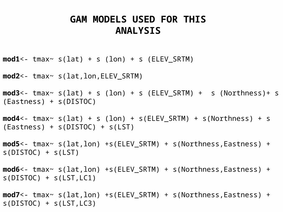
GAM MODELS USED FOR THIS ANALYSIS

mod1<- tmax~ s(lat) + s (lon) + s (ELEV_SRTM) mod2<- tmax~ s(lat,lon,ELEV_SRTM) mod3<- tmax~ s(lat) + s (lon) + s (ELEV_SRTM) + s (Northness)+ s (Eastness) + s(DISTOC) mod4<- tmax~ s(lat) + s (lon) + s(ELEV_SRTM) + s(Northness) + s (Eastness) + s(DISTOC) + s(LST) mod5<- tmax~ s(lat,lon) +s(ELEV_SRTM) + s(Northness,Eastness) + s(DISTOC) + s(LST)

mod6<- tmax~ s(lat,lon) +s(ELEV_SRTM) + s(Northness,Eastness) + s(DISTOC) + s(LST,LC1) mod7<- tmax~ s(lat,lon) +s(ELEV_SRTM) + s(Northness,Eastness) + s(DISTOC) + s(LST,LC3)

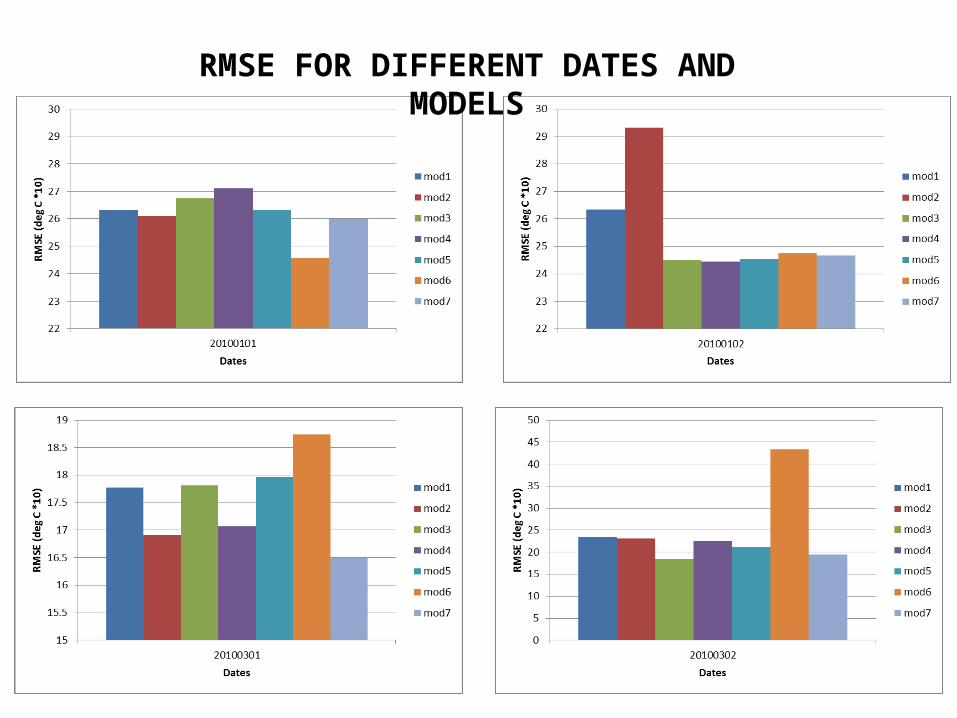
RMSE FOR DIFFERENT DATES AND MODELS

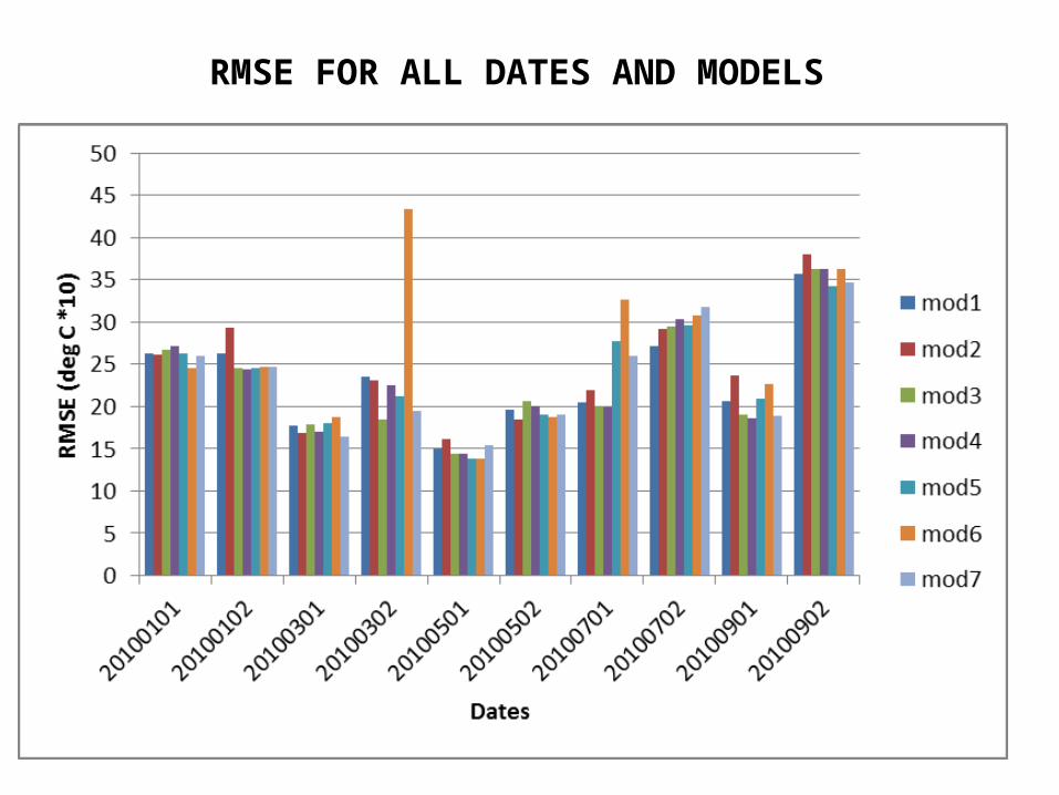
RMSE FOR ALL DATES AND MODELS

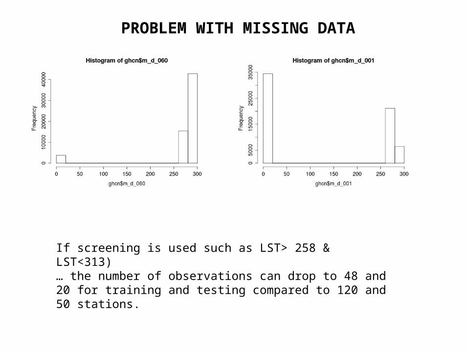
PROBLEM WITH MISSING DATA

If screening is used such as LST> 258 & LST<313)… the number of observations can drop to 48 and 20 for training and testing compared to 120 and 50 stations.

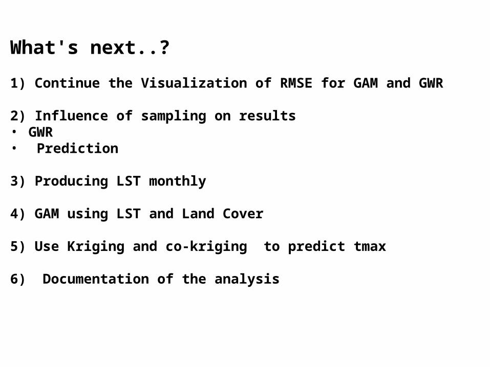
What's next..?

1) Continue the Visualization of RMSE for GAM and GWR

2) Influence of sampling on results• GWR • Prediction

3) Producing LST monthly

4) GAM using LST and Land Cover

5) Use Kriging and co-kriging to predict tmax

6) Documentation of the analysis