Environmental Impact of Solvents - mdmasearch.mdma.ch/picproxie_docs/000532906-14581_17.pdf · Environmental Impact of Solvents 17.1 THE ENVIRONMENTAL FATE AND MOVEMENT OF ORGANIC

17

Environmental Impact of

Solvents

17.1 THE ENVIRONMENTAL FATE AND MOVEMENT OF ORGANICSOLVENTS IN WATER, SOIL, AND AIRa

William R. Roy

Illinois State Geological Survey, Champaign, IL, USA

17.1.1 INTRODUCTION

Organic solvents are released into the environment by air emissions, industrial and

waste-treatment effluents, accidental spillages, leaking tanks, and the land disposal of sol-

vent-containing wastes. For example, the polar liquid acetone is used as a solvent and as an

intermediate in chemical production. ATSDR1 estimated that about 82 million kg of acetone

was released into the atmosphere from manufacturing and processing facilities in the U.S. in

1990. About 582,000 kg of acetone was discharged to water bodies from the same type of

facilities in the U.S. ATSDR2 estimated that in 1988 about 48,100 kg of tetrachloroethylene

was released to land by manufacturing facilities in the U.S.Once released, there are numerous physical and chemical mechanisms that will con-

trol how a solvent will move in the environment. As solvents are released into the environ-ment, they may partition into air, water, and soil phases. While in these phases, solventsmay be chemically transformed into other compounds that are less problematic to the envi-ronment. Understanding how organic solvents partition and behave in the environment hasled to better management approaches to solvents and solvent-containing wastes. There aremany published reference books written about the environmental fate of organic chemicalsin air, water, and soil.3-7 The purpose of this section is to summarize the environmental fateof six groups of solvents (Table 17.1.1) in air, water, and soil. A knowledge of the likelypathways for the environmental fate of organic solvents can serve as the technical basis forthe management of solvents and solvent-containing wastes.

aPublication authorized by the Chief, Illinois State Geological Survey

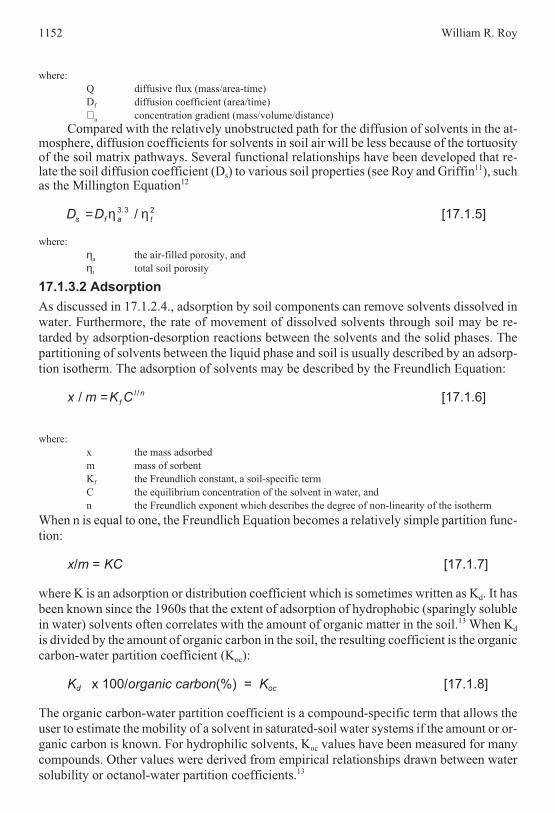
Table 17.1.1. The six groups of solvents discussed in this section

Alcoholsn-Butyl alcoholIsobutyl alcoholMethanol

Benzene DerivativesBenzeneChlorobenzeneo-Cresolo-DichlorobenzeneEthylbenzeneNitrobenzeneTolueneo-Xylene

Chlorinated Aliphatic HydrocarbonsCarbon tetrachlorideDichloromethaneTetrachloroethylene1,1,1-TrichloroethaneTrichloroethylene

Chlorinated FluorocarbonsTrichlorofluoromethane (F-11),1,1,2,2-Tetrachloro-1,2-difluoroethane ( F-112)1,1,2-Trichloro-1,2,2-trifluoroethane (F-113)1,2,-Dichlorotetrafluoroethane (F-114)

KetonesAcetoneCyclohexanoneMethyl ethyl ketoneMethy isobutyl ketone

OthersCarbon disulfideDiethyl etherEthyl acetateHexaneDecane (a major component of mineral spirits)PyridineTetrahydrofuran

17.1.2 WATER

17.1.2.1 Solubility

One of the most important properties of an organic solvent is its solubility in water. The

greater a compound's solubility, the more likely that a solvent or a solvent-containing waste

will dissolve into water and become part of the hydrological cycle. Hence, water solubility

can affect the extent of leaching of solvent wastes into groundwater, and the movement of

dissolved solvent into rivers and lakes. Aqueous solubility also determines the efficacy of

removal from the atmosphere through dissolution into precipitation. The solubility of sol-

vents in water may be affected by temperature, salinity, dissolved organic matter, and the

presence of other organic solvents.

17.1.2.2 Volatilization

Solvents dissolved in water may volatilize into the atmosphere or soil gases. A Henry's Law

constant (KH) can be used to classify the behavior of dissolved solvents. Henry's Law de-

scribes the ratio of the partial pressure of the vapor phase of an ideal gas (Pi) to its mole frac-

tion (Xi) in a dilute solution, viz.,

K P XH i i i( ) /= [17.1.1]

In the absence of measured data, a Henry's Law constant for a given solvent may be es-timated by dividing the vapor pressure of the solvent by its solubility in water (Si) at thesame temperature;

KH(i) = Pi (atm) / Si (mol/m3 solvent) [17.1.2]

A KH value of less than 10-4 atm-mol/m3 suggests that volatilization would probablynot be a significant fate mechanism for the dissolved solvent. The rate of volatilization is

1150 William R. Roy

more complex, and depends on the rate of flow, depth, and turbulence of both the body ofwater and the atmosphere above it. In the absence of measured values, there are a number ofestimation techniques to predict the rate of removal from water.8

17.1.2.3 Degradation

The disappearance of a solvent from solution can also be the result of a number of abiotic

and biotic processes that transform or degrade the compound into daughter compounds that

may have different physicochemical properties from the parent solvent. Hydrolysis, a

chemical reaction where an organic solvent reacts with water, is not one reaction, but a fam-

ily of reactions that can be the most important processes that determine the fate of many or-

ganic compounds.9 Photodegradation is another family of chemical reactions where the

solvent in solution may react directly under solar radiation, or with dissolved constituents

that have been made reactive by solar radiation. For example, the photolysis of water yields

a hydroxyl radical:

H O h HO H2 + → • +ν [17.1.3]

Other oxidants such as peroxy radicals (RO2r) and ozone can react with solvents inwater. The subject of photodegradation is treated in more detail under atmospheric pro-cesses (17.1.4).

Biodegradation is a family of biologically mediated (typically by microorganisms)conversions or transformations of a parent compound. The ultimate end-products ofbiodegradation are the conversion of organic compounds to inorganic compounds associ-ated with normal metabolic processes.10 This topic will be addressed under Soil (17.1.3.3).

17.1.2.4 Adsorption

Adsorption is a physicochemical process whereby a dissolved solvent may be concentrated

at solid-liquid interfaces such as water in contact with soil or sediment. In general, the ex-

tent of adsorption is inversely proportional to solubility; sparingly soluble solvents have a

greater tendency to adsorb or partition to the organic matter in soil or sediment (see Soil,

17.1.3.2).

17.1.3 SOIL


Volatilization from soil may be an important mechanism for the movement of solvents from

spills or from land disposed solvent-containing wastes. The efficacy and rate of volatiliza-

tion from soil depends on the solvent's vapor pressure, water solubility, and the properties of

the soil such as soil-water content, airflow rate, humidity, temperature and the adsorption

and diffusion characteristics of the soil.Organic-solvent vapors move through the unsaturated zone (the interval between the

ground surface and the water-saturated zone) in response to two different mechanisms; con-vection and diffusion. The driving force for convective movement is the gradient of totalgas pressure. In the case of diffusion, the driving force is the partial-pressure gradient ofeach gaseous component in the soil air. The rate of diffusion of a solvent in bulk air can bedescribed by Fick's Law, viz.,

Q Df a= − ∇ [17.1.4]

17.1 The environmental fate and movement of organic solvents 1151

where:

Q diffusive flux (mass/area-time)

Df diffusion coefficient (area/time)

∇ a concentration gradient (mass/volume/distance)

Compared with the relatively unobstructed path for the diffusion of solvents in the at-mosphere, diffusion coefficients for solvents in soil air will be less because of the tortuosityof the soil matrix pathways. Several functional relationships have been developed that re-late the soil diffusion coefficient (Ds) to various soil properties (see Roy and Griffin11), suchas the Millington Equation12

D Ds f a t= η η3 3 2. / [17.1.5]

where:

ηa the air-filled porosity, and

ηt total soil porosity

17.1.3.2 Adsorption

As discussed in 17.1.2.4., adsorption by soil components can remove solvents dissolved in

water. Furthermore, the rate of movement of dissolved solvents through soil may be re-

tarded by adsorption-desorption reactions between the solvents and the solid phases. The

partitioning of solvents between the liquid phase and soil is usually described by an adsorp-

tion isotherm. The adsorption of solvents may be described by the Freundlich Equation:

x m K Cf

l n/ /= [17.1.6]

where:

x the mass adsorbed

m mass of sorbent

Kf the Freundlich constant, a soil-specific term

C the equilibrium concentration of the solvent in water, and

n the Freundlich exponent which describes the degree of non-linearity of the isotherm

When n is equal to one, the Freundlich Equation becomes a relatively simple partition func-

tion:

x/m = KC [17.1.7]

where K is an adsorption or distribution coefficient which is sometimes written as Kd. It has

been known since the 1960s that the extent of adsorption of hydrophobic (sparingly soluble

in water) solvents often correlates with the amount of organic matter in the soil.13 When Kd

is divided by the amount of organic carbon in the soil, the resulting coefficient is the organic

carbon-water partition coefficient (Koc):

Kd x 100/organic carbon(%) = Koc [17.1.8]

The organic carbon-water partition coefficient is a compound-specific term that allows the

user to estimate the mobility of a solvent in saturated-soil water systems if the amount or or-

ganic carbon is known. For hydrophilic solvents, Koc values have been measured for many

compounds. Other values were derived from empirical relationships drawn between water

solubility or octanol-water partition coefficients.13

1152 William R. Roy


Solvents may be degraded in soil by the same mechanisms as those in water. In

biodegradation, microorganisms utilize the carbon of the solvents for cell growth and main-

tenance. In general, the more similar a solvent is to one that is naturally occurring, the more

likely that it can be biodegraded into other compound(s) because the carbon is more avail-

able to the microbes. Moreover, the probability of biodegradation increases with the extent

of water solubility of the compound. It is difficult to make generalities about the extent or

rate of solvent biodegradation that can be expected in soil. Biodegradation can depend on

the concentration of the solvent itself, competing processes that can make the solvent less

available to microbes (such as adsorption), the population and diversity of microorganisms,

and numerous soil properties such as water content, temperature, and reduction-oxidation

potential. The rate and extent of biodegradation reported in studies appears to depend on the

conditions under which the measurement was made. Some results, for example, were based

on sludge-treatment plant simulations or other biological treatment facilities that had been

optimized in terms of nutrient content, microbial acclimation, mechanical mixing of reac-

tants, or temperature. Hence, these results may overestimate the extent of biodegradation in

ambient soil in a spill or waste-disposal scenario.First-order kinetic models are commonly used to describe biodegradation because of

their mathematical simplicity. First-order biodegradation is to be expected when the organ-isms are not increasing in abundance. A first-order model also lends itself to calculating ahalf-life (t1/2) which is a convenient parameter to classify the persistence of a solvent. If asolvent has a soil half-life of 6 months, then about half of the compound will have degradedin six months. After one year, about one fourth the initial amount would still be present, andafter 3 half-lives (1.5 years), about 1/8 of the initial amount would be present.

Howard et al.14 estimated ranges of half-lives for solvents in soil, water, and air. Forsolvents in soil, the dominant mechanism in the reviewed studies may have beenbiodegradation, but the overall values are indicative of the general persistence of a solventwithout regard to the specific degradation mechanism(s) involved.

17.1.4 AIR


As introduced in 17.1.2.3, solvents may be photodegraded in both water and air. Atmo-

spheric chemical reactions have been studied in detail, particularly in the context of smog

formation, ozone depletion, and acid rain. The absorption of light by chemical species gen-

erates free radicals which are atoms, or groups of atoms that have unpaired electrons. These

free radicals are very reactive, and can degrade atmospheric solvents. Atmospheric ozone,

which occurs in trace amounts in both the troposphere (sea level to about 11 km) and in the

stratosphere (11 km to 50 km elevation), can degrade solvents. Ozone is produced by the

photochemical reaction:

O h O O2 + → +ν [17.1.9]

O O O M+ → +2 3 [17.1.10]

where M is another species such as molecular nitrogen that absorbs the excess energy given

off by the reaction. Ozone-depleting substances include the chlorofluorocarbons (CFC) and

carbon tetrachloride in the stratosphere.


17.1.4.2 Atmospheric residence time

Vapor-phase solvents can dissolve into water vapor, and be subject to hydrolysis reactions

and ultimately, precipitation (wet deposition), depending on the solubility of the given sol-

vent. The solvents may also be adsorbed by particulate matter, and be subject to dry deposi-

tion. Lyman16 asserted that atmospheric residence time cannot be directly measured; that it

must be estimated using simple models of the atmosphere. Howard et al.14 calculated ranges

in half-lives for various organic compounds in the troposphere, and considered reaction

rates with hydroxyl radicals, ozone, and by direct photolysis.

17.1.5 THE 31 SOLVENTS IN WATER

17.1.5.1 Solubility

The solubility of the solvents in Table 17.1.1 ranges from those that are miscible with water

to those with solubilities that are less than 0.1 mg/L (Table 17.1.2). Acetone, methanol,

pyridine and tetrahydrofuran will readily mix with water in any proportion. The solvents

that have an aqueous solubility of greater than 10,000 mg/L are considered relatively

hydrophillic as well. Most of the benzene derivatives and chlorinated fluorocarbons are rel-

atively hydrophobic. Hexane and decane are the least soluble of the 31 solvents in Table

17.1.1. Most material safety data sheets for decane indicate that the n-alkane is “insoluble”

and that the solubility of hexane is “negligible.” How the solubility of each solvent affects

its fate in soil, water, and air is illustrated in the following sections.

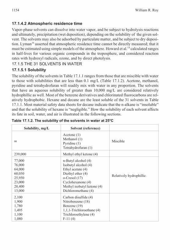
Table 17.1.2. The solubility of the solvents in water at 25oC

Solubility, mg/L Solvent (reference)

∞

Acetone (1)

Methanol (1)

Pyridine (1)

Tetrahydrofuran (1)

Miscible

239,000 Methyl ethyl ketone (4)

77,000

76,000

64,000

60,050

25,950

23,000

20,400

13,000

n-Butyl alcohol (4)

Isobutyl alcohol (4)

Ethyl acetate (4)

Diethyl ether (4)

o-Cresol (17)

Cyclohexanone (4)

Methyl isobutyl ketone (4)

Dichloromethane (4)

Relatively hydrophillic

2,100

1,900

1,780

1,495

1,100

1,080

Carbon disulfide (4)

Nitrobenzene (18)

Benzene (19)

1,1,1-Trichloroethane (4)

Trichloroethylene (4)

F-11 (4)

1154 William R. Roy

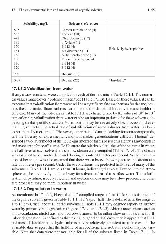
Solubility, mg/L Solvent (reference)

805

535

472

175

170

161

156

150

130

120

Carbon tetrachloride (4)

Toluene (20)

Chlorobenzene (17)

o-Xylene (4)

F-113 (4)

Ethylbenzene (17)

o-Dichlorobenzene (17)

Tetrachloroethylene (4)

F-114 (4)

F-112 (4)

Relatively hydrophobic

9.5 Hexane (21)

0.05 Decane (22) “Insoluble”

17.1.5.2 Volatilization from water

Henry's Law constants were compiled for each of the solvents in Table 17.1.1. The numeri-

cal values ranged over 7 orders of magnitude (Table 17.1.3). Based on these values, it can be

expected that volatilization from water will be a significant fate mechanism for decane, hex-

ane, the chlorinated fluorocarbons, carbon tetrachloride, tetrachloroethylene and trichloro-

ethylene. Many of the solvents in Table 17.1.1 are characterized by KH values of 10-3 to 10-2

atm-m3/mole; volatilization from water can be an important pathway for these solvents, de-

pending on the specific situation. Volatilization may be a relatively slow process for the re-

maining solvents. The actual rate of volatilization of some solvents from water has been

experimentally measured.4,17 However, experimental data are lacking for some compounds,

and the diversity of experimental conditions makes generalizations difficult. Thomas8 de-

scribed a two-layer model of the liquid-gas interface that is based on a Henry's Law constant

and mass-transfer coefficients. To illustrate the relative volatilities of the solvents in water,

the half-lives of each solvent in a shallow stream were compiled (Table 17.1.4). The stream

was assumed to be 1 meter deep and flowing at a rate of 1 meter per second. With the excep-

tion of hexane, it was also assumed that there was a breeze blowing across the stream at a

rate of 3 meters per second. Under these conditions, the predicted half-lives of many of the

solvents in Table 16.1.1 are less than 10 hours, indicating that volatilization into the atmo-

sphere can be a relatively rapid pathway for solvents released to surface water. The volatil-

ization of pyridine, isobutyl alcohol, and cyclohexanone may be a slow process, and other

fate processes may be more important in water.

17.1.5.3 Degradation in water

As mentioned in 17.1.3.3, Howard et al.14 compiled ranges of half-life values for most of

the organic solvents given in Table 17.1.1. If a “rapid” half-life is defined as in the range of

1 to 10 days, then about 12 of the solvents in Table 17.1.1 may degrade rapidly in surface

water by primarily biodegradation (Figures 17.1.1 and 17.1.2). Abiotic mechanisms such as

photo-oxidation, photolysis, and hydrolysis appear to be either slow or not significant. If

“slow degradation” is defined as that taking longer than 100 days, then it appears that F-11

and most of the chlorinated hydrocarbons may be relatively persistent in surface water. The

available data suggest that the half-life of nitrobenzene and isobutyl alcohol may be vari-

able. Note that data were not available for all of the solvents listed in Table 17.1.1. In


groundwater, the half-life values proposed

by Howard et al.14 appear to be more vari-

able than those for surface water. For exam-

ple, the half-life of benzene ranges from 10

days in aerobic groundwater to 2 years in

anaerobic groundwater.19 Such ranges in

half-lives make meaningful generalizations

difficult. However, it appears that metha-

nol, n-butyl alcohol, and other solvents (see

Figures 17.1.1 and 17.1.2) may biodegrade

in groundwater with a half-life that is less

than 60 days. As with surface water, the

chlorinated hydrocarbons may be relatively persistent in groundwater. Howard et al.14 cau-

tioned that some of their proposed half-life generalizations were based on limited data or

from screening studies that were extrapolated to surface and groundwater. Scow10 summa-

rized that it is currently not possible to predict rates of biodegradation because of a lack of

standardized experimental methods, and because the variables that control rates are not well

understood. Hence, Figures 17.1.1 and 17.1.2 should be viewed as a summary of the poten-

tial for each solvent to degrade, pending more site-specific information.

1156 William R. Roy

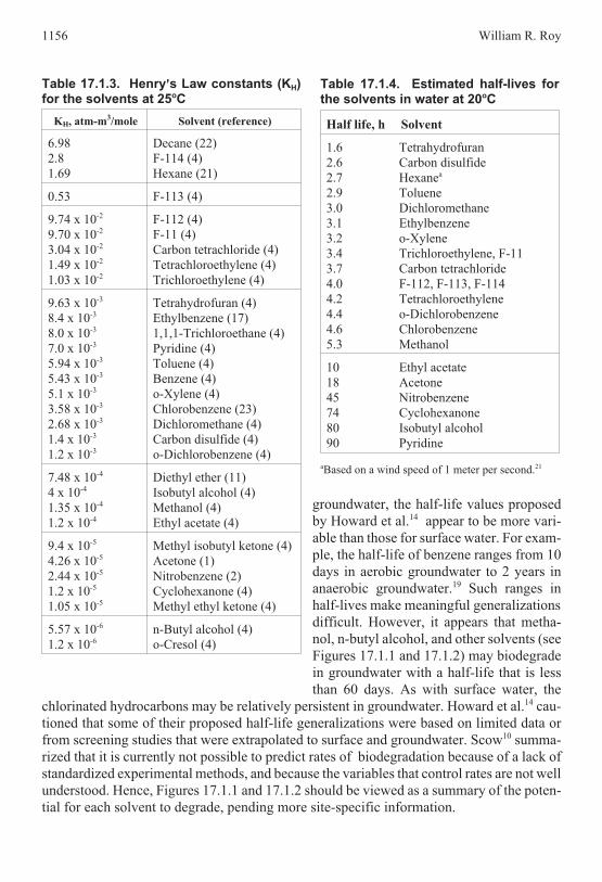
Table 17.1.3. Henry's Law constants (KH)for the solvents at 25oC

KH, atm-m3/mole Solvent (reference)

6.98

2.8

1.69

Decane (22)

F-114 (4)

Hexane (21)

0.53 F-113 (4)

9.74 x 10-2

9.70 x 10-2

3.04 x 10-2

1.49 x 10-2

1.03 x 10-2

F-112 (4)

F-11 (4)




9.63 x 10-3

8.4 x 10-3

8.0 x 10-3

7.0 x 10-3

5.94 x 10-3

5.43 x 10-3

5.1 x 10-3

3.58 x 10-3

2.68 x 10-3

1.4 x 10-3

1.2 x 10-3

Tetrahydrofuran (4)

Ethylbenzene (17)


Pyridine (4)

Toluene (4)

Benzene (4)

o-Xylene (4)

Chlorobenzene (23)

Dichloromethane (4)



7.48 x 10-4

4 x 10-4

1.35 x 10-4

1.2 x 10-4

Diethyl ether (11)

Isobutyl alcohol (4)

Methanol (4)

Ethyl acetate (4)

9.4 x 10-5

4.26 x 10-5

2.44 x 10-5

1.2 x 10-5

1.05 x 10-5


Acetone (1)

Nitrobenzene (2)

Cyclohexanone (4)

Methyl ethyl ketone (4)

5.57 x 10-6

1.2 x 10-6

n-Butyl alcohol (4)

o-Cresol (4)

Table 17.1.4. Estimated half-lives forthe solvents in water at 20oC

Half life, h Solvent

1.6 Tetrahydrofuran

2.6 Carbon disulfide

2.7 Hexanea

2.9 Toluene

3.0 Dichloromethane

3.1 Ethylbenzene

3.2 o-Xylene

3.4 Trichloroethylene, F-11

3.7 Carbon tetrachloride

4.0 F-112, F-113, F-114

4.2 Tetrachloroethylene

4.4 o-Dichlorobenzene

4.6 Chlorobenzene

5.3 Methanol

10 Ethyl acetate

18 Acetone

45 Nitrobenzene

74 Cyclohexanone

80 Isobutyl alcohol

90 Pyridine

aBased on a wind speed of 1 meter per second.21

17.1.6 SOIL


Soil diffusion coefficients were estimated for most of the solvents in Table 17.1.1. Using the

Millington Equation, the resulting coefficients (Table 17.1.5) ranged from 0.05 to 0.11

m2/day. Hence, there was little variation in magnitude between the values for these particu-

lar solvents. As discussed in Thomas24 the diffusion of gases and vapors in unsaturated soil

is a relatively slow process. The coefficients in Table 17.1.5 do not indicate the rate at which

olvents can move in soil; such rates must be either measured experimentally or predicted

using models that require input data such as soil porosity, moisture content, and the concen-

trations of the solvents in the vapor phase to calculate fluxes based solely on advective

movement. Variations in water content, for example, will control vapor-phase movement.

The presence of water can reduce the air porosity of soil, thereby reducing the soil diffusion

coefficient (Eq. 17.1.5). Moreover, relatively water-soluble chemicals may dissolve into

water in the vadose zone. Hence, water can act as a barrier to the movement of solvent va-

pors from the subsurface to the surface.Solvents spilled onto the surface of soil may volatilize into the atmosphere. The Dow

Method24 was used in this section to estimate half-life values of each solvent if spilled on thesurface of a dry soil. The Dow Method is a simple relationship that was derived for the evap-oration of pesticides from bare soil;

t1/2 (days) = 1.58 x 10-8 (KocS/Pv) [17.1.11]


Figure 17.1.1. The ranges in degradation half-lives for

the alcohols and benzene derivatives in surface water,

groundwater, and soil (data from Howard et al.14).

Figure 17.1.2. The ranges in degradation half-lives

for the chlorinated aliphatic hydrocarbons, F-11 and

F-113, and ketones in surface water, groundwater,

and soil (data from Howard et al.14).

where:

t1/2 evaporation half-life (days)

Koc organic carbon-water partition

coefficient (L/kg)

S solubility in water (mg/L), and

Pv vapor pressure (mm Hg at 20oC)

The resulting estimated half-life is in-versely proportional to vapor pressure; thegreater the vapor pressure, the greater theextent of volatilization. Conversely, therate of volatilization will be reduced if thesolvent readily dissolves into water or isadsorbed by the soil. Organic carbon-waterpartition coefficients were compiled foreach solvent (see 17.1.6.2.), and vaporpressure data (not shown) were collectedfrom Howard.4 The resulting half-life esti-mates (Table 17.1.6) indicated that volatil-ization would be a major pathway if theliquid solvents were spilled on soil; all ofthe half-life estimates were less than onehour. Thomas24 cautioned, however, thatsoil moisture, soil type, temperature, andwind conditions were not incorporated inthe simple Dow Model.

1158 William R. Roy

Table 17.1.5. Estimated soil diffusioncoefficients Ds (from Roy and Griffin11)

Solvent Ds, m2/day

n-Butyl alcohol 0.062 (25oC)

Isobutyl alcohol 0.050 (0oC)

Methanol 0.111 (25oC)

Benzene 0.060 (15oC)

Chlorobenzene 0.052 (30oC)

o-Cresol 0.053 (15oC)

o-Dichlorobenzene 0.049 (20oC)

Ethylbenzene 0.046 (0oC)

Nitrobenzene 0.050 (20oC)

Toluene 0.058 (25oC)

o-Xylene 0.049 (15oC)

Carbon tetrachloride 0.051 (25oC)

Dichloromethane 0.070 (15oC)

Tetrachloroethylene 0.051 (20oC)

1,1,1-Trichloroethane 0.075 (20oC)

Trichloroethylene 0.058 (15oC)

F-11 0.060 (15oC)

F-112 -

F-113 0.053 (15oC)

F-114 0.056 (15oC)

Acetone 0.076 (0oC)

Cyclohexanone -

Methyl ethyl ketone -

Methyl isobutyl ketone -

Carbon disulfide 0.074 (25oC)

Diethyl ether 0.054 (0oC)

Ethyl acetate 0.059 (25oC)

Hexane -

Mineral spirits -

Pyridine -

Tetrahydrofuran -

Table 17.1.6. Estimated soil-evapora-tion half lives

Solvent Half-life, min.

o-Cresol 38

Nitrobenzene 19

n-Butyl alcohol 18

Pyridine 8

Decane 4

Isobutanol

Cyclohexanone1

All other solvents <1

Table 17.1.7. The organic carbon-water partition coefficients (Koc) of the solvents at25oC

Koc, L/kg Solvent (reference)

<1 Methanol (13), Tetrahydrofurana

1

4

7

8

9

Acetone (13)

Methyl ethyl ketone (13)

Pyridine (13)

Ethyl acetate, isobutyl alcohol (13)

Diethyl ether (13)

Mobile

10

20

24

25

63

67

72

97

Cyclohexanone (13)

o-Cresol (17)


Dichloromethane (13)


Nitrobenzene (13)

n-Butyl alcohol (4)

Benzene (13)

110

152

155

164

242

303

318

343

363

372

437

457

479




Ethylbenzene (17)

Toluene (26)


Chlorobenzene (13)


o-Xylene (13)

F-113 (13)

F-114 (13)

F-112 (13)

F-11 (13)

Relatively mobile

1,950 Hexane (21)Relatively Immobile

57,100a Decane

aCalculated using the relationship logKoc = 3.95 - 0.62logS where S = water solubility in mg/L (see Hassett et al.25)

17.1.6.2 Adsorption

Organic carbon-water partition coefficients were compiled (Table 17.1.7) for each of the

solvents in Table 17.1.1. A Koc value is a measure of the affinity of a solvent to partition to

organic matter which in turn will control the mobility of the solute in soil and groundwater

under convective flow. Although the actual amount of organic matter will determine the ex-

tent of adsorption, a solvent with a Koc value of less than 100 L/kg is generally regarded as

relatively mobile in saturated materials. Hence, adsorption may not be a significant fate

mechanism for 16 of the solvents in Table 17.1.1. In contrast, adsorption by organic matter

may be a major fate mechanism controlling the fate of three of the benzene derivatives, and

most of the chlorinated compounds. Hexane and particularly decane would likely be rela-

tively immobile. However, when the organic C content of an adsorbent is less than about 1


g/kg, the organic C fraction is not a valid predictor of the partitioning of nonpolar organic

compounds,27 and other properties such as pH, surface area, or surface chemistry contribute

to or dominate the extent of adsorption. Moreover, pyridine occurs at a cation (pKa = 5.25)

over a wide pH range, and thus it is adsorbed by electrostatic interactions rather than by the

hydrophobic mechanisms that are endemic to using Koc values to predict mobility.The desorption of solvents from soil has not been extensively measured. In the appli-

cation of advection-dispersion models to predict solute movement, it is generally assumedthat adsorption is reversible. However, the adsorption of the solutes in Table 17.1.1 may notbe reversible. For example, hysteresis is often observed in pesticide adsorption-desorptionstudies with soils.28 The measurement and interpretation of desorption data for solid-liquidsystems is not well understood.29,30 Once adsorbed, some adsorbates may react further to be-come covalently and irreversibly bound, while others may become physically trapped in thesoil matrix.28 The non-singularity of adsorption-desorption may sometimes result from ex-perimental artifacts.28,31


As discussed in 17.1.3.3., Howard et al.14 also estimated soil half-life values (Figures 17.1.1

and 17.1.2) for the degradation of most of the solvents in Table 17.1.1. Biodegradation was

cited as the most rapid process available to degrade solvents in a biologically active soil.

The numerical values obtained were often the same as those estimated for surface water.

1160 William R. Roy

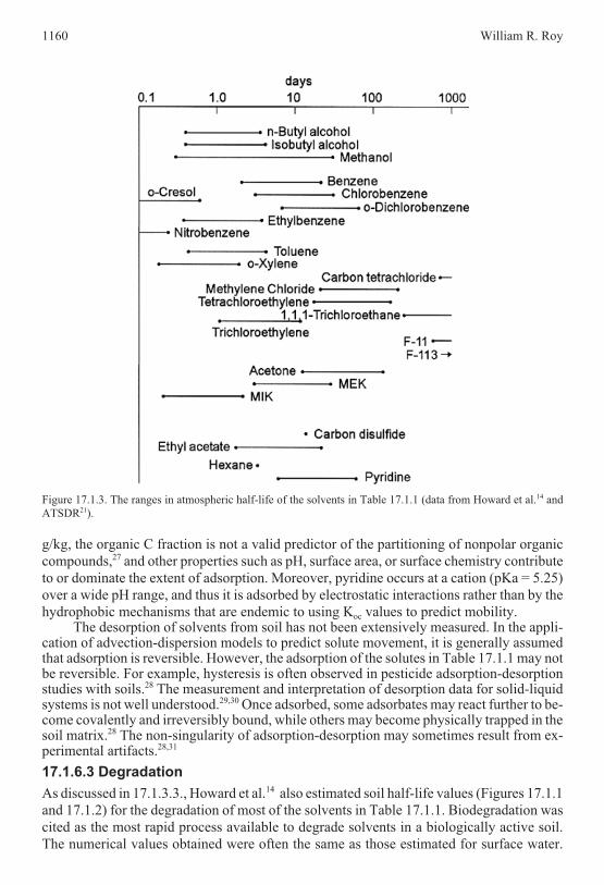
Figure 17.1.3. The ranges in atmospheric half-life of the solvents in Table 17.1.1 (data from Howard et al.14 and

ATSDR21).

Consequently, it appears likely that the alcohols, ketones, o-cresol, ethyl acetate, and

pyridine will degrade rapidly in soil if rapidly is defined as having a half-life of 10 days or

less. Most of the benzene derivatives, F-11, and the chlorinated aliphatic hydrocarbons may

be relatively persistent in soil. Analogous information was not located for diethyl ether,

hexane, decane, or tetrahydrofuran. ATSDR21 for example, found that there was little infor-

mation available for the degradation of n-hexane in soil. It was suggested that n-hexane can

degrade to alcohols, aldehydes, and fatty acids under aerobic conditions.

17.1.7 AIR

Once released into the atmosphere, the most rapid mechanism to attenuate most of the sol-

vents in Table 17.1.1 appears to be by photo-oxidation by hydroxyl radicals in the tropo-

sphere. Based on the estimates by Howard et al.,14 it appeared that nine of the solvents can

be characterized by an atmospheric residence half-life of 10 days or less (Figure 17.1.3).

The photo-oxidation of solvents yields products. For example, the reaction of OH radicals

with n-hexane can yield aldehydes, ketones, and nitrates.21

The reaction of some of the solvents with ozone may be much slower. For example,the half-life for the reaction of benzene with ozone may be longer than 100 years.19 Solventssuch as carbon tetrachloride, 1,1,1-trichloroethane, and the chlorinated fluorocarbons maybe relatively resistant to photo-oxidation. The major fate mechanism of atmospheric1,1,1-trichloroethane, for example, may be wet deposition.32

REFERENCES

1 Agency for Toxic Substances and Disease Registry. Toxicological Profile for Acetone. ATSDR, Atlanta,

Georgia, 1994.

2 Agency for Toxic Substances and Disease Registry. Toxicological Profile for Tetrachloroethylene. ATSDR,

Atlanta, Georgia, 1991.

3 D. Calamari (ed.) Chemical Exposure Predictions, Lewis Publishers, 1993.

4 P. H. Howard, Handbook of Environmental Fate and Exposure Data for Organic Chemicals. Vol. II

Solvents. Lewis Publishers, Chelsea, Michigan, 1990.

5 W. J. Lyman, W. F. Reehl, and D. H. Rosenblatt (eds). Handbook of Chemical Property Estimation

Methods, American Chemical Society, Washington, D.C., 1990.

6 R. E. Ney. Fate and Transport of Organic Chemicals in the Environment. 2nd ed. Government Institutes, Inc.

Rockville, MD, 1995.

7 B. L. Sawhney and K. Brown (eds.). Reactions and Movement of Organic Chemicals in Soils,

Soil Science Society of America, Special Publication Number 22, 1989.

8 R. G. Thomas, Volatilization From Water, W. J. Lyman, W. F. Reehl, and D. H. Rosenblatt (eds). in

Handbook of Chemical Property Estimation Methods, American Chemical Society, Washington, D.C,

Chap. 15, 1990.

9 J. C. Harris. Rate of Hydrolysis, Lyman, W. J., W. F. Reehl, and D. H. Rosenblatt (eds). in Handbook of

Chemical Property Estimation Methods, American Chemical Society, Washington, D.C, Chap. 7, 1990.

10 K. M. Scow, 1990, Rate of Biodegradation, W. J. Lyman, W. F. Reehl, and D. H. Rosenblatt (eds). in

Handbook of Chemical Property Estimation Methods, American Chemical Society, Washington, D.C,

Chap. 9, 1990.

11 W. R. Roy and R. A. Griffin, Environ. Geol. Water Sci., 15, 101 (1990).

12 R. J. Millington, Science, 130, 100 (1959).


14 P. H. Howard, R. S. Boethling, W. F. Jarvis, W. M. Meylan, and Edward M. Michalenko. Handbook of

Environmental Degradation Rates, Lewis Publishers, Chelsea, Michigan, 1991.

15 M. Alexander and K. M. Scow, Kinetics of Biodegradation, B. L. Sawhney, and K. Brown (eds.). in

Reactions and Movement of Organic Chemicals in Soils. Soil Science Society of America Special

Publication, Number 22, Chap. 10, 1989.

16 W. J. Lyman, Atmospheric Residence Time, W. J. Lyman, W. F. Reehl, and D. H. Rosenblatt (eds). in

Handbook of Chemical Property Estimation Methods. American Chemical Society, Washington, D.C,

Chap. 10, 1990.


17 P. H. Howard, Handbook of Environmental Fate and Exposure Data for Organic Chemicals. Vol. I.

Large Production and Priority Pollutants. Lewis Publishers, Chelsea, Michigan, 1989.

18 Agency for Toxic Substances and Disease Registry. Toxicological Profile for Nitrobenzene. ATSDR,


19 Agency for Toxic Substances and Disease Registry. Toxicological Profile for Benzene. ATSDR, Atlanta,

Georgia, 1991.

20 Agency for Toxic Substances and Disease Registry. Toxicological Profile for Toluene. ATSDR, Atlanta,

Georgia, 1998.

21 Agency for Toxic Substances and Disease Registry. Toxicological Profile for Hexane. ATSDR, Atlanta,

Georgia, 1997.

22 D. MacKay and W. Y. Shiu, J. Phys. Chem. Ref. Data, 4, 1175 (1981).

23 Agency for Toxic Substances and Disease Registry. Toxicological Profile for Chlorobenzene. ATSDR,


24 R. G. Thomas. Volatilization from Soil in W. J. Lyman, W. F. Reehl, and D. H. Rosenblatt (eds). Handbook

of Chemical Property Estimation Methods. American Chemical Society, Washington, D.C, Chap. 16,

1990.

25 J. J. Hassett, W. L. Banwart, and R. A. Griffin. Correlation of compound properties with soil sorption

characteristics of nonpolar compounds by soils and sediments; concepts and limitations In C. W. Francis and

S. I. Auerback (eds), Environmental and Solid Wastes, Characterization, Treatment, and Disposal,

Chap. 15, p. 161-178, Butterworth Publishers, London, 1983.

26 J. M. Gosset, Environ. Sci. Tech., 21, 202 (1987).

27 T. Stauffer W. G. MacIntyre. 1986, Tox. Chem., 5, 949 (1986).

28 W. C. Koskinen and S. S. Harper. The retention process, mechanisms. p. 51-77. In Pesticides in the Soil

Environment. Soil Science Society of America Book Series, no. 2, 1990.

29 R. E. Green, J. M. Davidson, and J. W. Biggar. An assessment of methods for determining

adsorption-desorption of organic chemicals. p. 73-82. In A. Bainn and U. Kafkafi (eds.), Agrochemicals in

Soils, Pergamon Press, New York, 1980.

30 R. Calvet, Environ. Health Perspectives, 83,145 (1989).

31 B. T. Bowman and W. W. Sans, J. Environ. Qual., 14, 270 (1985).

32 Agency for Toxic Substances and Disease Registry. Toxicological Profile for 1,1,1-Trichloroethane.

ATSDR, Atlanta, Georgia, 1989.

17.2 FATE-BASED MANAGEMENT OF ORGANICSOLVENT-CONTAINING WASTESa

William R. Roy

Illinois State Geological Survey, Champaign, IL, USA

17.2.1 INTRODUCTION

The wide spread detection of dissolved organic compounds in groundwater is a major envi-

ronmental concern, and has led to greater emphasis on incineration and waste minimization

when compared with the land disposal of solvent-containing wastes. The movement and en-

vironmental fate of dissolved organic solvents from point sources can be approximated by

the use of computer-assisted, solute-transport models. These models require information

about the composition of leachate plumes, and site-specific hydrogeological and chemical

1162 William R. Roy

aPublication authorized by the Chief, Illinois State Geological Survey

data for the leachate-site system. A given land-disposal site has a finite capacity to attenuate

organic solvents in solution to environmentally acceptable levels. If the attenuation capac-

ity of a site can be estimated, then the resulting information can be used as criteria to make

decisions as to what wastes should be landfilled, and what quantities of solvent in a given

waste can be safely accepted. The purpose of this section is to summarize studies1-3 that

were conducted that illustrate how knowledge of the environmental fate and movement of

the solvents in Section 17.1 can be used in managing solvent-containing wastes. These stud-

ies were conducted by using computer simulations to assess the fate of organic compounds

in leachate at a waste-disposal site.

17.2.1.1 The waste disposal site

There are three major factors that will ultimately determine the success of a land-disposal

site in being protective of the environment with respect to groundwater contamination by

organic solvents: (1) the environmental fate and toxicity of the solvent; (2) the mass loading

rate, i.e., the amount of solvent entering the subsurface during a given time, and (3) the total

amount of solvent available to leach into the groundwater. The environmental fate of the

solvents was discussed in 17.1.The hypothetical waste-disposal site used in this evaluation (Figure 17.2.1) had a sin-

gle waste trench having an area of 0.4 hectare. Although site-specific dimensions may be as-signed with actual sites, this hypotheticalsite was considered representative of manysituations found in the field. The trench was12.2 meters (40 ft) deep and was con-structed with a synthetic/compacted-soildouble-liner system. The bottom of thetrench was in direct contact with a sandyaquifer that was 6.1 meters (20 ft) thick.The top of the water table was defined asbeing at the top of the sandy aquifer. Thus,this site was designed as a worst-case sce-nario. The sandy aquifer directly beneaththe hazardous-waste trench would offer lit-tle resistance to the movement of contami-nants. To further compound a worst-casesituation, it was also assumed that the entiretrench was saturated with leachate, generat-ing a 12.2 meter (40 ft) hydraulic headthrough the liner. This could correspond toa situation where the trench had completelyfilled with leachate because the leachatecollection system had either failed or thesite had been abandoned.

The following aquifer properties, typ-ical of sandy materials,1 were used in thestudy:

17.2 Fate-based management 1163

Figure 17.2.1. Design of the waste-disposal site model

used in the simulations (Roy et al.1).

saturated hydraulic conductivity = 10-3 cm/secsaturated volumetric water content = 0.36 cm3/cm3

dry bulk density = 1.7 g/cm3

hydraulic gradient = 0.01 cm/cmmean organic carbon content = 0.18%These aquifer properties yield a groundwater flow rate of 9.3 meters (30 ft) per year.

The direction of groundwater flow is shown in Figure 17.2.1 to be from left to right. Theedge of the disposal trench was 154 meters (500 ft) from a monitoring well that was open tothe entire thickness of the aquifer. This monitoring well served as a worst-case receptor be-cause it was placed in the center of the flow path at the site boundary and it served as thecompliance point for the site. The downgradient concentrations of organic solvents at thecompliance well, as predicted by a solute-transport model, were used to evaluate whetherthe attenuation capacity of the site was adequate to reduce the contaminants to acceptableconcentrations before they migrated beyond the compliance point.

17.2.1.2 The advection-dispersion model and the required input

The 2-dimensional, solute-transport computer program PLUME was used to conduct con-

taminant migration studies. Detailed information about PLUME, including boundary con-

ditions and quantitative estimates of dispersion and groundwater dilution, were summarized

by Griffin and Roy.3 In this relatively simple and conservative approach, PLUME did not

take into account volatilization from water. Volatilization is a major process for many of the

solvents (see Section 17.1). Adsorption was assumed to be reversible, and soil-water parti-

tion coefficients were calculated by assuming that the aquifer contained 0.18% organic car-

bon (see Roy and Griffin4). A degradation half-life was assigned to each solvent (Table

17.2.1). In many cases, conservative half-life values were used. For example, all of the ke-

tones were assigned a half-life of 5 years, which is much longer than those proposed for ke-

tones in groundwater (see Section 17.1). The movement of each solvent was modeled

separately whereas it should be recognized that solvents in mixtures may have different

chemical properties that can ultimately affect their fate and movement.

17.2.1.3 Maximum permissible concentrations

Central to the type of assessment is a definition of an environmentally acceptable concentra-

tion of each contaminant. These acceptable levels were defined as Maximum Permissible

Concentrations (MPC), and were based on the toxicological assessments of solvents in

drinking water by George and Siegel.5 These MPC levels (Table 17.2.1) are not the same

levels as the current Maximum Contaminant Levels (MCL) that were promulgated by the

U.S. Environmental Protection Agency for drinking water.

17.2.1.4 Distribution of organic compounds in leachate

An initial solute concentration must be selected for the application of solute transport mod-

els. An initial concentration for each solvent was based on the chemical composition of

leachates from hazardous-waste sites.1 Where available, the largest reported concentration

was used in the modeling efforts (Table 17.2.1). No published data were located for some of

the solvents such as cyclohexanone. In such cases, the initial concentration was arbitrarily

assigned as 1,000 mg/L or it was equated to the compound's solubility in water. Hexane,

decane, and tetrahydofuran were not included in these studies.The amount of mass of each organic compound entering the aquifer via the dou-

ble-liner system was calculated using these initial leachate concentrations. There was a con-tinuous 12.2-meter head driving the leachate through the liner. Leachate was predicted to

1164 William R. Roy

break through the liner in 30 years. Under these conditions, approximately 131,720L/year/acre of leachate would seep through the liner. The assumptions used in deriving thisflow estimate were summarized in Roy et al.1

Table 17.2.1. The six groups of solvents discussed in this section, theircorresponding Maximum Permissible Concentrations (MPC), the largest reportedconcentrations in leachate (LC), and the assigned half-lives from Roy et al.1

MPC, µg/L LC, mg/L Half-life, years

Alcohols

n-Butyl alcohol 2,070 1,000 5

Isobutyl alcohol 2,070 1,000 5

Methanol 3,600 42.4 5

Benzene Derivatives

Benzene 1.6 7.37 20

Chlorobenzene 488 4.62 20

o-Cresol 304 0.21 20

o-Dichlorobenzene 400 0.67 50

Ethylbenzene 1,400 10.1 10

Nitrobenzene 19,800 0.74 20

Toluene 14,300 100 10

o-Xylene 14,300 19.7 10

Chlorinated Aliphatic Hydrocarbons

Carbon tetrachloride 0.4 25.0 50

Dichloromethane 0.19 430 20

Tetrachloroethylene 0.80 8.20 20

1,1,1-Trichloroethane 6.00 590 50

Trichloroethylene 2.70 260 20

Chlorinated Fluorocarbons

Trichlorofluoromethane (F-11) 0.19 0.14 50

1,1,2,2-Tetrachloro-1,2-difluoroethane ( F-112) 0.19 120 50

1,1,2-Trichloro-1,2,2-trifluoroethane (F-113) 0.19 170 stable

1,2,-Dichlorotetrafluoroethane (F-114) 0.19 130 stable

Ketones

Acetone 35,000 62 5

Cyclohexanone 3,500 1,000 5

Methyl ethyl ketone 30,000 53.0 5


MPC, µg/L LC, mg/L Half-life, years

Methyl isobutyl ketone 143 10.0 5

Others

Carbon disulfide 830 1,000 10

Diethyl ether 55,000 1,000 5

Ethyl acetate 55,000 1,000 5

Pyridine 207 1,000 20

A mass-loading rate was conservatively calculated for each solvent as,

M Q Clr l= × [17.2.1]

where:

Mlr the mass loading rate (mass/time/area),

Q calculated leachate flux (131.7 kL/year/hectare), and

Cl largest concentration of the solvent in leachate (mg/L)

17.2.2 MOVEMENT OF SOLVENTS IN GROUNDWATER

Ketones and alcohols have little tendency to be adsorbed by soil materials (see Section

17.1), and would appear at the compliance point only a few years after liner breakthrough

(Figure 17.2.2). Because the mass loading rates were held constant, the ketones and alco-

hols assumed maximum steady-state concentrations after approximately 40 to 50 years

(Figure 17.2.3). These two classes of organic solvents degrade readily, reducing their

downgradient concentrations. The distribution of the benzene derivatives at the compliance

well depended substantially on their soil-water partition coefficients, their tendencies to de-

1166 William R. Roy

Figure 17.2.2. The predicted distribution of methyl ethyl

ketone (mg/L) in the aquifer 100 years after the leachate

has broken through the liner (Griffin and Roy3).

Figure 17.2.3. The predicted concentrations of methyl

ethyl ketone, methanol, benzene, 1,1,1-trichloroetha-

ne, ethyl acetate, and F-22 at the compliance point as a

function of time (Roy et al.1).

grade, and the initial concentrations. Under the conditions described, the relative

steady-state concentrations of the benzene derivatives were: toluene > benzene > chloro-

benzene > p-xylene > nitrobenzene > o-dichlorobenzene > o-cresol > ethyl benzene. Methy-

lene chloride and 1,1,1-trichlorethane would dominate the chlorinated hydrocarbons.

Among the group of unrelated organic solvents, the concentration of pyridine at the well

was predicted to increase rapidly. Pyridine would eventually dominate this group in the rel-

ative order: pyridine > carbon disulfide > ethyl acetate > diethyl ether. The relative order of

fluorocarbons at the compliance well in terms of concentration was: F-21, F-22 >> F-12 >

F-113 > F-114 > F-112 > R-112a > FC-115 >> F-11.In brief, the computer simulations predicted that all 28 organic compounds would

eventually migrate from the waste trench, and be detected at the compliance well. The pre-dicted concentrations varied by four orders of magnitude, and were largely influenced bythe initial concentrations used in calculating the mass loading rate to the aquifer.

17.2.3 MASS LIMITATIONS

The next step in this analysis was to determine whether these predicted concentrations

would pose an environmental hazard by evaluating whether the site was capable of attenuat-

ing the concentrations of the organic compounds to levels that are protective of human

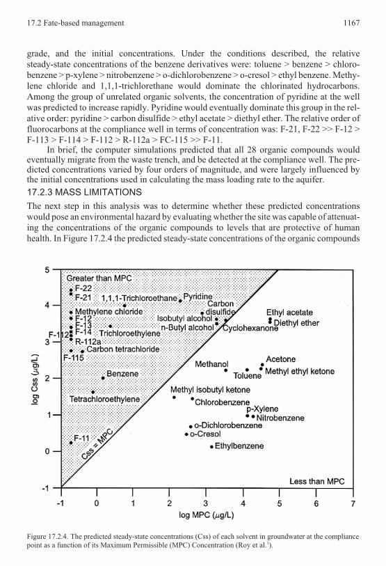
health. In Figure 17.2.4 the predicted steady-state concentrations of the organic compounds


Figure 17.2.4. The predicted steady-state concentrations (Css) of each solvent in groundwater at the compliance

point as a function of its Maximum Permissible (MPC) Concentration (Roy et al.1).

in groundwater at the compliance well were plotted against their MPCs. The boundary

shown in Figure 17.2.4 represents the situation where the steady-state concentration (Css)

equals the MPC. Consequently, the predicted Css is less than its corresponding MPC when

the Css of a given compound plots in the lower-right side. In this situation, these organic

compounds could enter the aquifer at a constant mass loading rate without exceeding the at-

tenuation capacity of the site. The steady-state concentrations of twenty solvents exceeded

their corresponding MPCs. The continuous addition of these organic compounds (i.e., a

constant mass loading rate) would exceed the site's ability to attenuate them to environmen-

tally acceptable levels in this worst-case scenario. There are two avenues for reducing the

steady-state concentrations downgradient from the trench: (1) reduce the mass loading rate,

and/or (2) reduce the mass of organic compound available to leach into the aquifer. Be-

cause, the RCRA-required double liner was regarded as the state-of-the-art with respect to

liner systems, it was not technically feasible to reduce the volume of leachate seeping into

the aquifer under the conditions imposed. The worst-case conditions could be relaxed by as-

suming a lower leachate head in the landfill or by providing a functional leachate-collection

system. Either condition would be reasonable and would reduce the mass loading rate. An-

other alternative is to reduce the mass available for leaching. In the previous simulations,

the mass available to enter the aquifer was assumed to be infinite. Solute transport models

can be used to estimate threshold values for the amounts of wastes initially landfilled.2 A

threshold mass (Mt) can be derived so that the down-gradient, steady-state concentrations

will be less than the MPC of the specific compound, viz.,

Mt = V(MPC x 1000) t [17.2.2]

where:

Mt the threshold mass in g/hectare

V the volume of leachate entering the aquifer in L/yr/hectare

MPC the maximum permissible concentration as g/L, and

t time in years; the amount of time between liner breakthrough and when the predicted

concentration of the compound in the compliance well equals its MPC.

Using this estimation technique, Roy et al.1 estimated mass limitations for the com-pounds that exceeded their MPCs in the simulations. They found that benzene, carbon tetra-chloride, dichloromethane, pyridine, tetrachloroethylene, 1,1,1-trichloroethylene,trichloroethylene and all chlorinated fluorocarbons would require strict mass limitations(<250 kg/ha). Other solvents could be safely landfilled at the site without mass restrictions:acetone, chlorobenzene, cresols, o-dichlorobenzene, diethyl ether, ethyl acetate,ethylbenzene, methanol, methyl ethyl ketone, methyl isobutyl ketone, nitrobenzene, tolu-ene, and xylene. Some solvents (cyclohexanone, n-butyl alcohol, isobutyl alcohol, and car-bon disulfide) would require some restrictions to keep the attenuation capacity of the sitefrom being exceeded.

These studies,1-3 demonstrated that the land disposal of wastes containing some or-ganic solvents at sites using best-available liner technology may be environmentally accept-able. Wastes that contain chlorinated hydrocarbons, however, may require pretreatmentsuch as incineration or stabilization before land disposal. If the mass-loading rate is con-trolled and the attenuation capacity of the site is carefully studied, the integrated andmultidisciplinary approach outlined in this section can be applied to the management of sol-vent-containing wastes.

1168 William R. Roy

REFERENCES

1 W. R. Roy, R. A. Griffin, J. K. Mitchell, and R. A. Mitchell, Environ. Geol. Water Sci., 13, 225 (1989).

2 W. R. Roy and R. A. Griffin, J. Haz. Mat., 15, 365 (1987).

3 R. A. Griffin and W. R. Roy. Feasibility of land disposal of organic solvents: Preliminary Assessment.

Environmental Institute for Waste Management Studies, Report No. 10, University of Alabama, 1986.


5 W. J. George and P. D. Siegel. Assessment of recommended concentrations of selected organic solvents in

drinking water. Environmental Institute for Waste Management Studies, Report No. 15, University of

Alabama, 1988.

17.3 ENVIRONMENTAL FATE AND ECOTOXICOLOGICAL EFFECTSOF GLYCOL ETHERS

James Devillers

CTIS, Rillieux La Pape, France

Aurélie Chezeau, André Cicolella, and Eric Thybaud

INERIS, Verneuil-en-Halatte, France

17.3.1 INTRODUCTION

Glycol ethers and their acetates are widely used as solvents in the chemical, painting, print-

ing, mining and furniture industries. They are employed in the production of paints, coat-

ings, resins, inks, dyes, varnishes, lacquers, cleaning products, pesticides, deicing additives

for gasoline and jet fuel, and so on.1 In 1997, the world production of glycol ethers was

about 900,000 metric tons.2

There are two distinct series of glycol ethers namely the ethylene glycol ethers whichare produced from ethylene oxide and the propylene glycol ethers derived from propyleneoxide. The former series is more produced and used than the latter. Thus, inspection of the42,000 chemical substances recorded by INRS (France) in the SEPIA data bank, between1983 and 1998, reveals that 10% of them include ethylene glycol ethers and about 4% pro-pylene glycol ethers.2 However, due to the reproductive toxicity of some ethylene glycolmonoalkyl ethers,3-5 it is important to note that the worldwide tendency is to replace thesechemicals by glycol ethers belonging to the propylenic series.2

Given the widespread use of glycol ethers, it is obvious that these chemicals enter theenvironment in substantial quantities. Thus, for example, the total releases to all environ-mental media in the United States for ethylene glycol monomethyl ether and ethylene glycolmonoethyl ether in 1992 were 1688 and 496 metric tons, respectively.6 However, despitethe potential hazard of these chemicals, the problems of the environmental contaminationswith glycol ethers have not received much attention. There are two main reasons for this.First, these chemicals are not classified as priority pollutants, and hence, their occurrence inthe different compartments of the environment is not systematically investigated. Thus, forexample, there are no glycol ethers on the target list for the Superfund hazardous waste sitecleanup program.6 Second, glycol ethers are moderately volatile colorless liquids with ahigh water solubility and a high solubility with numerous solvents. Consequently, the clas-

17.3 Environmental fate of glycol ethers 1169

sical analytical methods routinely used for detecting the environmental pollutants do notprovide reliable results with the glycol ethers, especially in the aquatic environments.

Under these conditions, the aim of this chapter is to review the available literature onthe occurrence, environmental fate, and ecotoxicity of glycol ethers.

17.3.2 OCCURRENCE

Despite the poor applicability of the most widely used USEPA analytical methods, some

ethylene, diethylene, and triethylene glycol ethers have been reported as present in

Superfund hazardous waste sites in the US more often than some of the so-called priority

pollutants.6 More specifically, Eckel and co-workers6 indicated that in Jacksonville

(Florida), a landfill received a mixture of household waste and wastes from aircraft mainte-

nance and paint stripping from 1968 to 1970. In 1984, sampling of residential wells in the

vicinity revealed concentrations of 0.200, 0.050, and 0.010 mg/l of diethylene glycol di-

ethyl ether, ethylene glycol monobutyl ether, and diethylene glycol monobutyl ether, re-

spectively. One year later, concentrations of 0.050 to 0.100 mg/l of diethylene glycol

diethyl ether were found in the most contaminated portion of the site. In 1989, some sam-

ples still indicated the presence of diethylene glycol diethyl ether and triethylene glycol

dimethyl ether. This case study clearly illustrates that glycol ethers may persist in the envi-

ronment for many years after a contamination. Concentrations of 0.012 to 0.500 mg/l of eth-

ylene glycol monobutyl ether were also estimated in residential wells on properties near a

factory (Union Chemical, Maine, USA) manufacturing furniture stripper containing

N,N-dimethylformamide. In addition, in one soil sample located in that site, a concentration

of 0.200 mg/kg of ethylene glycol monobutyl ether was also found. In another case study,

Eckel and co-workers6 showed that ethylene glycol diethyl ether was detected with esti-

mated concentrations in the range from 0.002 to 0.031 mg/l in eight residential wells adja-

cent to a landfill (Ohio) receiving a mixture of municipal waste and various industrial

wastes, many of them from the rubber industry. Last, ethylene glycol monomethyl ether

was detected in ground-water samples at concentrations of 30 to 42 mg/l (Winthrop landfill,

Maine).6

In 1991, the high resolution capillary GC-MS analysis of a municipal wastewater col-lected from the influent of the Asnières-sur-Oise treatment plant located in northern subur-ban Paris (France) revealed the presence of ethylene glycol monobutyl ether (0.035 mg/l),diethylene glycol monobutyl ether (0.015 mg/l), propylene glycol monomethyl ether (0.070mg/l), dipropylene glycol monomethyl ether (0.050 mg/l), and tripropylene glycolmonoethyl ether (<0.001 mg/l).7 In the Hayashida River (Japan) mainly polluted byeffluents from leather factories, among the pollutants separated by vacuum distillation andidentified by GS-MS, ethylene glycol monobutyl ether, ethylene glycol monoethyl ether,and diethylene glycol monobutyl ether were found at concentrations of 5.68, 1.20, and 0.24mg/l, respectively.8

In air samples collected in the pine forest area of Storkow (30 km south east of Berlin,Germany), the “Mediterranean Macchia” of Castel Porziano (Italy), and the Italian stationlocated at the foot of Everest (Nepal), GC-MS analysis showed concentrations of ethyleneglycol monobutyl ether of 1.25, 0.40, and 0.10 to 1.59 µg/m3, respectively.9

1170 J Devillers, A Chezeau, A Cicolella, E Thybaud

17.3.3 ENVIRONMENTAL BEHAVIOR

Due to their high water solubilities and low 1-octanol/water partition coefficients (log P),

the glycol ethers, after release in the environment, will be preferentially found in the aquatic

media and their accumulation in soils, sediments, and biota will be negligible.The available literature data on the biodegradation of glycol ethers reveal that most of

these chemicals are biodegradable under aerobic conditions (Table 17.3.1), suggesting thecompounds would not likely persist.

Table 17.3.1. Aerobic biodegradation of glycol ethers and their acetates in aquaticenvironments and soils

Name [CAS RN], Values Comments Ref.

Ethylene glycol monomethyl ether [109-86-4]

5 d = 30% bio-oxidation, 10 d = 62%,

15 d = 74%, 20 d = 88%

filtered domestic wastewater, non-acclimated seed, 3, 7,

10 mg/l (at least two), fresh water10

5 d = 6% bio-oxidation, 10 d = 18%,

15 d = 23%, 20 d = 39%


10 mg/l (at least two), salt water10

ThOD = 1.68 g/g, BOD5 = 0.12 g/g,

%ThOD = 7, COD = 1.69 g/g,

%ThOD = 101

effluent from a biological sanitary waste treatment

plant, 20 ± 1°C, unadapted seed, BOD = APHA SM

219, COD = ASTM D 1252-67

11

BOD5 = 0.50 g/g, %ThOD = 30 same conditions, adapted seed 11

Ethylene glycol monomethyl ether acetate [110-49-6]

ThOD = 1.63 g/g, BOD5 = 0.49 g/g,

%ThOD = 30, COD = 1.60 g/g,

%ThOD = 98


plant, 20 ± 1°C, unadapted seed, BOD = APHA SM 219,

COD = ASTM D 1252-67

11

Ethylene glycol monoethyl ether [110-80-5]

5 d = 36% bio-oxidation, 10 d = 88%,

15 d = 92%, 20 d = 100%




15 d = 50%, 20 d = 62%



ThOD = 1.96 g/g, BOD5 = 1.03 g/g,

%ThOD = 53, COD = 1.92 g/g,

%ThOD = 98




11


COD removed = 91.7% mixed culture, acclimation in a semi-continuous system 12

BOD5 = 0.353 g/g, BOD/ThOD = 18.1% fresh water, standard dilution method, 10 mg/l 13

BOD5 = 0.021 g/g, BOD/ThOD = 1.1% sea water, 10 mg/l 13

Ethylene glycol monoethyl ether acetate [111-15-9]

5 d = 36% bio-oxidation, 10 d = 79%,

15 d = 82%, 20 d = 80%



5 d = 10% bio-oxidation, 10 d = 44%,

15 d = 59%, 20 d = 69%





ThOD = 1.82 g/g, BOD5 = 0.74 g/g,

%ThOD = 41, COD = 1.76 g/g,

%ThOD = 96




11



Ethylene glycol diethyl ether [629-14-1]

ThOD = 2.31 g/g, BOD10 = 0.10 g/g 14

Ethylene glycol monoisopropyl ether [109-59-1]

ThOD = 2.15 g/g, BOD5 = 0.18 g/g,

%ThOD = 8, COD = 2.08 g/g, %ThOD = 97




11

Ethylene glycol monobutyl ether [111-76-2]

5 d = 26% bio-oxidation, 10 d = 74%,

15 d = 82%, 20 d = 88%



5 d = 29% bio-oxidation, 10 d = 64%,

15 d = 70%, 20 d = 75%



ThOD = 2.31 g/g, BOD5 = 0.71 g/g,

%ThOD = 31, COD = 2.20 g/g,

%ThOD = 95




11





5 d = 47% bio-oxidation, 15 d = 70%,

28 d = 75%

OECD Closed-Bottle test 301D, no prior acclima-

tion/adaptation of seed, 20°C15

28 d = 95% removal of DOCOECD 301E, 10 mg/l, non-adapted domestic activated

sludge16

28 d = 100% removalOECD 302B, 500 mg/l, non-adapted domestic activated

sludge16

1 d = 22% removal, 3 d = 63%, 5 d = 100%OECD 302B, 450 mg/l, non-adapted domestic activated

sludge16

14 d = 96% BOD of ThOD 100 mg/l, activated sludge 16

Ethylene glycol monobutyl ether acetate [112-07-2]

>90% DOC removal in 28 d OECD 302B, Zahn-Wellens test 16

Diethylene glycol monomethyl ether [111-77-3]

ThOD = 1.73 g/g, BOD5 = 0.12 g/g,

%ThOD = 7, COD = 1.71 g/g, %ThOD = 99

effluent from a biological sanitary waste treatmentplant, 20 ± 1°C, unadapted seed, BOD = APHA SM 219,COD = ASTM D 1252-67

11



BOD5 = 0.95 mmol/mmolacclimated mixed culture, estimated by linear regres-

sion technique from a 20-day test17

Diethylene glycol monomethyl ether acetate [629-38-9]

ThOD = 1.68 g/g, BOD10 = 1.10 g/g 14

Diethylene glycol monoethyl ether [111-90-0]

5 d = 17% bio-oxidation, 10 d = 71%,

15 d = 75%, 20 d = 87%



5 d = 11% bio-oxidation, 10 d = 44%,

15 d = 57%, 20 d = 70%



ThOD = 1.91 g/g, BOD5 = 0.20 g/g,

%ThOD = 11, COD = 1.85 g/g,

%ThOD = 97




11



BOD5 = 5.50 mmol/mmol acclimated mixed culture 17

Diethylene glycol diethyl ether [112-36-7]

ThOD = 2.17 g/g, BOD10 = 0.10 g/g 14

Diethylene glycol monobutyl ether [112-34-5]

ThOD = 2.17 g/g, BOD5 = 0.25 g/g,

%ThOD = 11, COD = 2.08 g/g,

%ThOD = 96




11


BOD5 = 5.95 mmol/mmol acclimated mixed culture 17

5 d = 27% bio-oxidation, 10 d = 60%,

15 d = 78%, 20 d = 81%

BOD APHA SM, no prior acclimation/adaptation of

seed, 20°C15


28 d = 88%,

OECD Closed-Bottle test 301D, no prior acclima-

tion/adaptation of seed, 20°C15

28 d >60% removalOECD 301C, modified MITI test, adapted activated

sludge16

28 d = 58% removalOECD 301C, modified MITI test, adapted activated

sludge16

1 d = 14% removal, 3 d = 19%, 5 d = 60%,

6 d = 100%

OECD 302B, modified Zahn-Wellens test, industrial

non-adapted activated sludge16

9 d = 100% removalOECD 302B, modified Zahn-Wellens test, non-adapted

activated sludge16

14 d = 94% removalOECD 301A, domestic secondary effluent sewage,

DOC measured16



BOD5 = 0.05 g/g (5.2% ThOD),

BOD10 = 0.39 g/g (57% ThOD),

BOD20 = 1.08 g/g (72% ThOD)

16

BOD = 0.25 g/g, COD = 2.08 g/g Dutch standard method, adapted sewage 16

Diethylene glycol monobutyl ether acetate [124-17-4]

BOD5 = 13.3% ThOD, BOD10 = 18.4%,

BOD15 = 24.6%, BOD20 = 67%16

Triethylene glycol monoethyl ether [112-50-5]


15 d = 63%, 20 d = 71%




15 d = 12%, 20 d = 22%



ThOD = 1.89 g/g, BOD5 = 0.05 g/g,

%ThOD = 3, COD = 1.84 g/g, %ThOD = 97




11


BOD5 = 1.15 mmol/mmolacclimated mixed culture, estimated by linear regres-

sion technique from a 20-day test17

Triethylene glycol monobutyl ether [143-22-6]


Propylene glycol monomethyl ether [107-98-2]

50% removal: <1 d (0.2 ppm), <2 d (9.9

ppm), <5 d (100 ppm)

sand = 72%, silt = 16%, clay = 12%, OC = 2.5%,

9.9 x 106 bacteria/g of soil18

50% removal: <1 d (0.4 ppm), <7 d (100

ppm)

sand = 74%, silt = 12%, clay = 14%, OC = 2.0%,


50% removal: <4 d (0.4 ppm), >56 d (100

ppm), <23 d (100 ppm with nutrients)

sand = 94%, silt = 4%, clay = 2%, OC = 0.4%,


BOD20 = 58% of ThOD 18

Propylene glycol monomethyl ether acetate [108-65-6]

50% removal: <1 d (2.5 ppm), <1 d (20

ppm),

sand = 72%, silt = 16%, clay = 12%, OC = 2.5%,


50% removal: <1 d (20 ppm)sand = 74%, silt = 12%, clay = 14%, OC = 2.0%,


50% removal: <1 d (20 ppm)sand = 94%, silt = 4%, clay = 2%, OC = 0.4%,





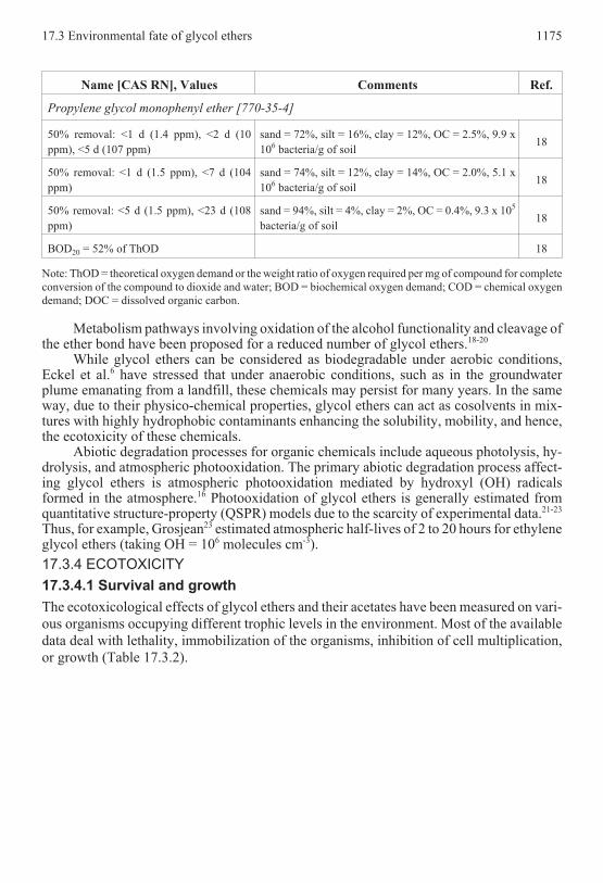
Propylene glycol monophenyl ether [770-35-4]

50% removal: <1 d (1.4 ppm), <2 d (10

ppm), <5 d (107 ppm)

sand = 72%, silt = 16%, clay = 12%, OC = 2.5%, 9.9 x

106 bacteria/g of soil18

50% removal: <1 d (1.5 ppm), <7 d (104

ppm)

sand = 74%, silt = 12%, clay = 14%, OC = 2.0%, 5.1 x

106 bacteria/g of soil18

50% removal: <5 d (1.5 ppm), <23 d (108

ppm)

sand = 94%, silt = 4%, clay = 2%, OC = 0.4%, 9.3 x 105

bacteria/g of soil18


Note: ThOD = theoretical oxygen demand or the weight ratio of oxygen required per mg of compound for complete

conversion of the compound to dioxide and water; BOD = biochemical oxygen demand; COD = chemical oxygen

demand; DOC = dissolved organic carbon.

Metabolism pathways involving oxidation of the alcohol functionality and cleavage ofthe ether bond have been proposed for a reduced number of glycol ethers.18-20

While glycol ethers can be considered as biodegradable under aerobic conditions,Eckel et al.6 have stressed that under anaerobic conditions, such as in the groundwaterplume emanating from a landfill, these chemicals may persist for many years. In the sameway, due to their physico-chemical properties, glycol ethers can act as cosolvents in mix-tures with highly hydrophobic contaminants enhancing the solubility, mobility, and hence,the ecotoxicity of these chemicals.

Abiotic degradation processes for organic chemicals include aqueous photolysis, hy-drolysis, and atmospheric photooxidation. The primary abiotic degradation process affect-ing glycol ethers is atmospheric photooxidation mediated by hydroxyl (OH) radicalsformed in the atmosphere.16 Photooxidation of glycol ethers is generally estimated fromquantitative structure-property (QSPR) models due to the scarcity of experimental data.21-23

Thus, for example, Grosjean23 estimated atmospheric half-lives of 2 to 20 hours for ethyleneglycol ethers (taking OH = 106 molecules cm-3).

17.3.4 ECOTOXICITY

17.3.4.1 Survival and growth

The ecotoxicological effects of glycol ethers and their acetates have been measured on vari-

ous organisms occupying different trophic levels in the environment. Most of the available

data deal with lethality, immobilization of the organisms, inhibition of cell multiplication,

or growth (Table 17.3.2).


Table 17.3.2. Effects of glycol ethers and their acetates on survival and growth oforganisms

Species Results Comments Ref.

Ethylene glycol monomethyl ether [109-86-4]

Bacteria

Pseudomonas putida 16-h TGK >10000 mg/ltoxicity threshold, inhibition of cell

multiplication24

Pseudomonas

aeruginosa4-m biocidal = 5-10% tested in jet fuel and water mixtures 25

Sulfate-reducing bacteria 3-m biocidal = 5-10% tested in jet fuel and water mixtures 25

Blue-green

algaeMicrocystis aeruginosa 8-d TGK = 100 mg/l

toxicity threshold, inhibition of cell

multiplication26

AlgaeScenedesmus

quadricauda8-d TGK >10000 mg/l


multiplication26

Yeasts Candida sp. 4-m biocidal = 5-10% tested in jet fuel and water mixtures 25

FungiCladosporium resinae

4-m biocidal = 10-17%

42-d NG = 20%

tested in jet fuel and water mixtures

NG = no visible mycelial growth

and spore germination, 1% glu-

cose-mineral salts medium, 30°C

25

27

Gliomastix sp. 4-m biocidal = 17-25% tested in jet fuel and water mixtures 25

Protozoa

Chilomonas

paramaecium48-h TGK = 2.2 mg/l


multiplication28

Uronema parduczi 20-h TGK > 10000 mg/ltoxicity threshold, inhibition of cell

multiplication29

Entosiphon sulcatum 72-h TGK = 1715 mg/ltoxicity threshold, inhibition of cell

multiplication30

Coelente-

rates

Hydra vulgaris

(syn. H. attenuata)72-h LC50 = 29000 mg/l semi-static, adult polyps 31

CrustaceaDaphnia magna

24-h LC50 >10000 mg/l

24-h EC50 >10000 mg/l

static, nominal concentrations

static, nominal concentrations, im-

mobilization

32

33

Artemia salina 24-h TLm >10000 mg/l static, 24.5°C 10

Fish

Carassius auratus 24-h TLm >5000 mg/lstatic, 20 ± 1°C, measured concen-

trations34

Leuciscus idus

melanotus

48-h LC50 >10000 mg/l

48-h LC0 >10000 mg/l

48-h LC100 >10000

mg/l

static (Juhnke) 35

Oryzias latipes24-h LC50 >1000 mg/l

48-h LC50 >1000 mg/l

static, same results at 10, 20, and

30°C36



Fish

Pimephales promelas

20% mortality = 50 mg/l,

0% mortality = 100 mg/l,

30% mortality = 200

mg/l,

70% mortality = 500

mg/l,

70% mortality = 700

mg/l,

100% mortality = 1000

mg/l

static with daily renewal, adults,

7-d of exposure37

Poecilia reticulata 7-d LC50 = 17434 mg/lsemi-static, 22 ± 1°C, rounded

value38

Lepomis macrochirus 96-h LC50 >10000 mg/lstatic, nominal concentrations,

L = 33-75 mm39

Menidia beryllina 96-h LC50 >10000 mg/lstatic, sea water, nominal concen-

trations, L = 40-100 mm39

Amphibia Xenopus laevis

0% mortality=2500

mg/l, 0% mortality =

7500 mg/l, 0% mortality

= 15000 mg/l

static with daily renewal, adults, 4-d

of exposure37

Ethylene glycol monomethyl ether acetate [110-49-6]

Fish

Carassius auratus 24-h TLm = 190 mg/lstatic, 20 ± 1°C, measured concen-

trations34

Lepomis macrochirus 96-h LC50 = 45 mg/lstatic, nominal concentrations,

L = 33-75 mm39

Menidia beryllina 96-h LC50 = 40 mg/lstatic, sea water, nominal concen-


Ethylene glycol monoethyl ether [110-80-5]

Bacteria

Pseudomonas aeruginosa 4-m biocidal = 5-10% tested in jet fuel and water mixtures 25


Vibrio fischeri

5-min EC50 = 376 mg/l,

15-min EC50 = 403

mg/l, 30-min

EC50 = 431 mg/l

reduction in light output, 15°C 40


Fungi Cladosporium resinae


42-d NG = 10%





25

27




Coelente-

rates

Hydra vulgaris



24-h EC50 = 54000 mg/l

48-h EC50 = 7671 mg/l


mobilization

static, 22 ± 1°C, nominal concentra-

tions, immobilization

41

42


Fish


trations34


value38

Lepomis macrochirus 96-h LC50 >10000 mg/lstatic, nominal concentrations,

L = 33-75 mm39

Menidia beryllina 96-h LC50 >10000 mg/lstatic, sea water, nominal concen-


Ethylene glycol monoethyl ether acetate [111-15-9]

Crustacea Artemia salina 24-h TLm = 4000 mg/l static, 24.5°C 10

Fish Carassius auratus 24-h TLm = 160 mg/lstatic, 20 ± 1°C, measured concen-

trations34

Ethylene glycol monopropyl ether [2807-30-9]

BacteriaPseudomonas aeruginosa 4-m biocidal = 0-2% tested in jet fuel and water mixtures 25



FungiCladosporium resinae 4-m biocidal = 2-5% tested in jet fuel and water mixtures 25


Ethylene glycol monoisopropyl ether [109-59-1]

Fungi Cladosporium resinae 42-d NG = 10%



cose-mineral salts medium, 30°C27

Fish


trations34


value38

Ethylene glycol monobutyl ether [111-76-2]

Bacteria

Pseudomonas putida 16-h TGK = 700 mg/ltoxicity threshold, inhibition of cell

multiplication24

Pseudomonas


Sulfate-reducing

bacteria3-m biocidal = 1-2% tested in jet fuel and water mixtures 25



Blue-green



multiplication26

Algae

Scenedesmus

quadricauda8-d TGK = 900 mg/l


multiplication26

Selenastrum

capricornutum

7-d EC50 >1000 mg/l,

NOEC = 125 mg/l,

LOEC = 250 mg/l

growth rate inhibition 16



4-m biocidal = 2-3%

42-d NG = 5%





25

27


Protozoa

Chilomonas

paramaecium48-h TGK = 911 mg/l


multiplication28

Uronema parduczi 20-h TGK = 463 mg/ltoxicity threshold, inhibition of cell

multiplication29


multiplication30

Coelente-

rates

Hydra vulgaris


Mollusca Crassostrea virginica

24-h LC50 = 181 mg/l

(143 - 228), 48-h

LC50 = 160 mg/l (125 -

204), 72-h LC50 = 114

mg/l (93.9 - 138), 96-h

LC50 = 89.4 mg/l

(72 - 110)

static, 22 ± 1°C, 10 organisms/tank 43


24-h LC50 = 1720 mg/l,

24-h LC0 = 1140 mg/l,

24-h LC100 = 2500 mg/l

24-h EC50 = 1815 mg/l

(1698-1940),

24-h EC0 = 1283 mg/l,

24-h EC100 = 2500 mg/l

48-h EC50 = 835 mg/l



mobilization

static, immobilization

32

33

16

Artemia salina 24-h TLm = 1000 mg/l static, 24.5°C 10



Crustacea Panaeus setiferus

24-h LC50 > 430 mg/l,

48-h LC50 = 173 mg/l

(123 - 242),

72-h LC50 = 147 mg/l

(116 - 186),

96-h LC50 = 130 mg/l

(104 - 162)

static, average size = 1.5 cm 43

Fish


trations34

Leuciscus idus

melanotus

48-h LC50 = 1575 mg/l,

48-h LC0 = 1350 mg/l

48-h LC100 = 1620 mg/l

48-h LC50 = 1395 mg/l,

48-h LC0 = 1170 mg/l,

48-h LC100 = 1490 mg/l

static (Juhnke)

static (Lüdemann) 35

Pimephales promelas 96-h LC50 = 2137 mg/l static 16


value38

Notropis atherinoides 72-h LC50 >500 mg/l static 16

Lepomis macrochirus

96-h LC50 = 1490 mg/l

24-h LC50 = 2950 mg/l,

96-h LC50 = 2950 mg/l

static, nominal concentrations,

L = 33-75 mm

39

44

Cyprinodon variegatus

24-h LC50 = 149 mg/l

(125 - 176),

48-h LC50 = 126 mg/l

(107 - 147),

72-h LC50 = 121 mg/l

(105 - 138),

96-h LC50 = 116 mg/l

(100 - 133)

static, 22 ± 1°C 43



Ethylene glycol dibutyl ether [112-48-1]





27

Diethylene glycol monomethyl ether [111-77-3]

Bacteria

Pseudomonas






Algae

Scenedesmus

subspicatus

72-h EC50 > 500 mg/l,

72-h EC20 > 500 mg/l,

72-h EC90 > 500 mg/l

biomass 45

Selenastrum

capricornutum96-h EC50 > 1000 mg/l biomass 45



42-d NG = 20%





25

27

Gliomastix sp. 4-m biocidal > 25% tested in jet fuel and water mixtures 25

Crustacea Daphnia magna

24-h LC50 = 1495 mg/l

(1300 - 1600),

48-h LC50 = 1192 mg/l

(1100 - 6500)

static, nominal concentrations 45

Fish

Oncorhynchus mykiss 96-h LC50 > 1000 mg/l semi-static, nominal concentrations 45


trations34

Pimephales promelas

24-h LC50 = 6400 mg/l

(6200 - 6600),

48-h LC50 = 6000 mg/l

(6000 -6100),

72-h LC50 = 6000 mg/l

(6000 -6100),

96-h LC50 = 5700 mg/l

(5600 - 5900)

static 45


L = 33-75 mm39

Diethylene glycol dimethyl ether [111-96-6]





27

Diethylene glycol monoethyl ether [111-90-0]

Bacteria Vibrio fischeri

5-min EC50 = 1000

mg/l,

5-min EC50 = 1290 mg/l

15-min EC50 = 10954

mg/l (10592.8 - 11327.5)

reduction in light output, nominal

concentrations

46

47





27

Coelente-

rates

Hydra vulgaris




Crustacea

Daphnia magna

48-h LC50 = 4670 mg/l

(3620 - 6010),

48-h LC50 = 3340 mg/l

(2120 - 5280)

static, 21.1°C, measured concentra-

tions

static, 23.3°C, measured concentra-

tions

48

Orconectes immunis96-h LC50 = 34700 mg/l

(29100 - 41400)

flow-through, 15.5°C, 0.47 g, mea-

sured concentrations48


Insecta Tanytarsus dissimilis 48-h LC50 = 18800 mg/lstatic, 22.3°C, measured concentra-

tions48

Echinoder-

mataArbacia punctulata

4-h EC50 = 10661 mg/l

(5576.5 - 20895.9)

1-h EC50 = 3370 mg/l

(3145.4 - 3610.8)

5-h EC50 = 4116 mg/l

(3408 - 4907)

static, marine, early embryo growth,

nominal concentrations

static, marine, sperm cell, nominal

concentrations

static, marine, increase in DNA,

nominal concentrations

47

47

49

Fish

Oncorhynchus mykiss96-h LC50 = 13400 mg/l

(11400 - 15700)



Carassius auratus

24-h TLm >5000 mg/l

96-h LC50 = 20800 mg/l

(15700 - 27500)

static, 20 ± 1°C, measured concen-

trations


sured concentrations

34

48

Gambusia affinis

96-h LC50 = 15200 mg/l

(12400 - 18700)

96-h LC50 = 12900 mg/l

(11100 - 15000)





48

Ictalurus punctatus 96-h LC50 = 6010 mg/lflow-through, 17.3°C, 0.72 g, mea-


Lepomis macrochirus

96-h LC50 >10000 mg/l

96-h LC50 = 21400 mg/l

(19100 - 23900)

static, nominal concentrations,

L = 33-75 mm



39

48

Pimephales promelas

96-h LC50 = 13900 mg/l

(11600 - 16700)

96-h LC50 = 9650 mg/l

(7910 - 11800)





48

Menidia beryllina 96-h LC50 >10000 mg/lstatic, sea water, nominal

concentrations, L = 40-100 mm39

Amphibia Rana catesbeiana96-h LC50 = 20900 mg/l

(19400 -22600)

flow-through, 17.2°C, 3.54 g,

measured concentrations48

Diethylene glycol diethyl ether [112-36-7]

Fungi Cladosporium resinae 42-d NG = 20%NG = no visible mycelial growthand spore germination, 1% glu-cose-mineral salts medium, 30°C

27



Diethylene glycol monobutyl ether [112-34-5]

Bacteria Pseudomonas putida

16-h TGK = 255 mg/l

16-h EC10 = 1170 mg/l


multiplication

growth inhibition, 25 ± 2°C

24

50

Blue-green



multiplication26

Algae

Scenedesmus

quadricauda8-d TGK = 1000 mg/l


multiplication26

Scenedesmus

subspicatus96-h EC50 > 100 mg/l limit test 50





27

Protozoa

Chilomonas

paramaecium48-h TGK = 2774 mg/l


multiplication28

Uronema parduczi 20-h TGK = 420 mg/ltoxicity threshold, inhibition of cell

multiplication29


multiplication30

Crustacea Daphnia magna

24-h LC50 = 2850 mg/l,

24-h LC0 = 1750 mg/l,

24-h LC100 = 3850 mg/l

24-h EC50 = 3200 mg/l

(2990-3424),

24-h EC0 = 2333 mg/l,

24-h EC100 = 5000 mg/l

48-h EC50 >100 mg/l

48-h NOEC >100 mg/l



mobilization

directive 84/449/ EEC, C2

32

33

16

Fish


trations34

Leuciscus idus

melanotus

48-h LC50 = 1805 mg/l,

48-h LC0 = 1140 mg/l,

48-h LC100 = 2185 mg/l

48-h LC50 = 2304 mg/l,

48-h LC0 = 1820 mg/l,

48-h LC100 = 2400 mg/l

48-h LC50 = 2750 mg/l

static (Juhnke)

static (Lüdemann)

static

35

35

16

Poecilia reticulata 7-d LC50 = 1149 mg/l semi-static, 22±1°C, rounded value 38


L = 33-75 mm39





Triethylene glycol monomethyl ether [112-35-6]

Bacteria

Pseudomonas


Sulfate-reducing





Triethylene glycol monoethyl ether [112-50-5]

Bacteria

Pseudomonas


Sulfate-reducing





Crustacea Artemia salina 24-h TLm >10000 mg/l static, 24.5°C 10

Fish Carassius auratus 24-h TLm >5000 mg/lstatic, 20 ± 1°C, measured concen-

trations34

Propylene glycol monomethyl ether [107-98-2]





27

Propylene glycol monomethyl ether acetate [108-65-6]

Fish Lepomis macrochirus24-h LC50 = 206 mg/l

96-h LC50 = 164 mg/l44

It is difficult to draw definitive conclusions from the data listed in Table 17.3.2. In-deed, most of the data have been retrieved from rather old studies performed without GLPprotocols. In addition, the toxicity values are generally based on nominal concentrationsand the endpoints are different. However, from the data listed in Table 17.3.2, it appears thatdespite a difference of sensibility among species, glycol ethers do not present acute and sub-acute ecotoxicological effects to the majority of the tested organisms. However, it is inter-esting to note that the acetates seem to be more toxic that the corresponding parentcompounds.10,34,39,51 In mammals, the acute toxicity of glycol ethers is also relatively low.The main target organs are the central nervous and haematopoitic systems. However, on thebasis of the available data no significant difference exists between the acute toxicity of gly-col ethers and their corresponding acetates.52


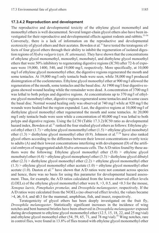
17.3.4.2 Reproduction and development

The reproductive and developmental toxicity of the ethylene glycol monomethyl and

monoethyl ethers is well documented. Several longer-chain glycol ethers also have been in-

vestigated for their reproductive and developmental effects against rodents and rabbits.53-56

Conversely, there is a lack of information on the reproductive and developmental

ecotoxicity of glycol ethers and their acetates. Bowden et al.31 have tested the teratogenic ef-

fects of four glycol ethers through their ability to inhibit the regeneration of isolated diges-

tion regions of Hydra vulgaris (syn. H. attenuata). They have shown that the concentrations

of ethylene glycol monomethyl, monoethyl, monobutyl, and diethylene glycol monoethyl

ethers that were 50% inhibitory to regenerating digestive regions (IC50) after 72-h of expo-

sure were 19,000, 1400, 540, and 19,000 mg/l, respectively. More specifically, at 10,000

mg/l of ethylene glycol monomethyl ether, the digestive regions regenerated the mouth and

some tentacles. At 19,000 mg/l only tentacle buds were seen, while 38,000 mg/l produced

disintegration of the coelenterates. Ethylene glycol monoethyl ether at 900 mg/l allowed the

regeneration of the mouth, some tentacles and the basal disc. At 1900 mg/l four digestive re-

gions showed wound healing while the remainder were dead. A concentration of 3700 mg/l

was lethal to both polyps and digestive regions. At concentrations up to 370 mg/l of ethyl-

ene glycol monobutyl ether, digestive regions regenerated some tentacles and in some cases

the basal disc. Normal wound healing only was observed at 740 mg/l while at 920 mg/l the

wounds were healed but the region expanded. Last, the digestive regions at 10,000 mg/l of

diethylene glycol monoethyl ether regenerated the mouth and some tentacles. At 20,000

mg/l only tentacle buds were seen while a concentration of 40,000 mg/l was lethal to both

polyps and digestive regions. Using the LC50 (Table 17.3.2)/IC50 ratio as developmental

hazard index, Bowden et al.31 ranked the four studied glycol ethers as follows: Ethylene gly-

col ethyl ether (1.7) > ethylene glycol monomethyl ether (1.5) > ethylene glycol monobutyl

ether (1.3) > diethylene glycol monoethyl ether (0.9). Johnson et al.57,58 have also ranked

glycol ethers according to the difference between their lowest concentrations overtly toxic

to adults (A) and their lowest concentrations interfering with development (D) of the artifi-

cial embryos of reaggregated adult Hydra attenuata cells. The A/D ratios found by these au-

thors were the following: Ethylene glycol monoethyl ether (5.0) > ethylene glycol

monobutyl ether (4.4) > ethylene glycol monophenyl ether (3.3) > diethylene glycol dibutyl

ether (2.3) > diethylene glycol monoethyl ether (2.2) > ethylene glycol monomethyl ether

(1.3) > ethylene glycol monomethyl ether acetate (1.0) = ethylene glycol monoethyl ether

acetate (1.0). Daston et al.37 have shown that A/D ratios were not constant across species

and hence, there was no basis for using this parameter for developmental hazard assess-

ment. Thus, for example, the A/D ratios calculated from the lowest observed effect levels

(LOELs) of the ethylene glycol monomethyl ether were 8, >3, 0.5, and <0.3 for the mouse,

Xenopus laevis, Pimephales promelas, and Drosophila melanogaster, respectively. If the

A/D ratios were calculated from the NOELs (no observed effect levels), the values became

>4, ≥6, 0.4, and ≤0.3 for the mammal, amphibian, fish, and insect, respectively.Teratogenicity of glycol ethers has been deeply investigated on the fruit fly,

Drosophila melanogaster. Statistically significant increases in the incidence of wingnotches and bent humeral bristles have been observed in Drosophila melanogaster exposedduring development to ethylene glycol monomethyl ether (12.5, 15, 18, 22, and 25 mg/vial)and ethylene glycol monoethyl ether (54, 59, 65, 71, and 78 mg/vial).59 Wing notches, rarein control flies, were found in 13.8% of flies treated with ethylene glycol monomethyl ether


(7.5µl/g).60 In general, male pupae are much more affected by ethylene glycol monomethylether than female pupae. However, teratogenicity appears strain dependent. Higher detoxi-fication occurs with increased alcohol dehydrogenase (ADH) activity. Ethylene glycolmonomethyl ether is much more toxic than its oxidation product, methoxyacetic acid, at thelevel of adult eclosion. Teratogenic effects were observed in an ADH-negative strain inspite of lacking ADH activity suggesting that apparently, ethylene glycol monomethyl etheris a teratogenic compound by itself against Drosophila melanogaster.61 Last, it is interestingto note that recently, Eisses has shown62 that administration of ethylene glycol monomethylether to larvae of fruit fly, containing the highly active alcohol dehydrogenase variantADH-71k, exposed the mitotic germ cells and the mitotic somatic cells of the imaginal discssimultaneously to the mutagen methoxyacetaldehyde and the teratogen methoxyacetic acid,respectively. Consequently, the chances for specific gene mutations, though non-adaptive,were likely increased by a feedback mechanism.

17.3.5 CONCLUSION

Despite their widespread use, glycol ethers and their acetates have received little attention

as potential environmental contaminants. Based on their physico-chemical properties, they

would tend to remain in the aquatic ecosystems where their bioconcentration, biomagnifi-

cation and sorption onto sediments will appear negligible. Volatilization from water and hy-

drolysis or photolysis in the aquatic ecosystems are generally of minimal importance.

Glycol ethers are also poorly sorbed to soil and their rapid removal in the atmosphere is ex-

pected. While glycol ethers are biodegradable under aerobic conditions, these chemicals

may persist for many years under anaerobic conditions.Based on the available acute ecotoxicity data, glycol ethers and their acetates can be

considered as practically non-toxic. However, there is a lack of information on theirlong-term effects on the biota. This is particularly annoying because the developmental tox-icity of some of them has been clearly identified against mammals. Consequently, there is aneed for studies dealing with the potential long-term effects of these chemicals against or-ganisms occupying different trophic levels in the environment in order to see whether or notthe classical methodological frameworks used for assessing the environmental risk ofxenobiotics remain acceptable for this class of chemicals.

17.3.6 ACKNOWLEDGMENT

This study was supported by the French Ministry of the Environment as part of the

PNETOX program (1998).

REFERENCES

1 R.J. Smialowicz, Occup. Hyg., 2, 269 (1996).

2 Anonymous in Ethers de Glycols. Quels Risques pour la Santé?, INSERM, Paris, 1999, pp. 1-19.

3 K. Nagano, E. Nakayama, M. Koyano, H. Oobayashi, H. Adachi, and T. Yamada, Jap. J. Ind. Health, 21, 29

(1979).


5 A. Cicolella, Cahiers de Notes Documentaires, 148, 359 (1992).

6 W. Eckel, G. Foster, and B. Ross, Occup. Hyg., 2, 97 (1996).

7 D.K. Nguyen, A. Bruchet, and P. Arpino, J. High Resol. Chrom., 17, 153 (1994).

8 A. Yasuhara, H. Shiraishi, M. Tsuji, and T. Okuno, Environ. Sci. Technol., 15, 570 (1981).

9 P. Ciccioli, E. Brancaleoni, A. Cecinato, R. Sparapani, and M. Frattoni, J. Chromatogr., 643, 55 (1993).

10 K.S. Price, G.T. Waggy, and R.A. Conway, J.Water Pollut. Control Fed., 46, 63 (1974).

11 A.L. Bridié, C.J.M. Wolff, and M. Winter, Water Res., 13, 627 (1979).

12 T. Fuka, V. Sykora, and P. Pitter, Sci. Pap. Inst. Chem. Technol. Praze Technol. Water, F25, 203 (1983) (in

Czech).

13 S. Takemoto, Y. Kuge, and M. Nakamoto, Suishitsu Odaku Kenkyu, 4, 22 (1981) (in Japanese).


14 P. Pitter and J. Chudoba, Biodegradability of Organic Substances in the Aquatic Environment, CRC Press,

Boca Raton, 1990.

15 G.T. Waggy, R.A. Conway, J.L. Hansen, and R.L. Blessing, Environ. Toxicol. Chem., 13, 1277 (1994).

16 C.A. Staples, R.J. Boatman, and M.L. Cano, Chemosphere, 36, 1585 (1998).

17 L. Babeu and D.D. Vaishnav, J. Ind. Microbiol., 2, 107 (1987).

18 S.J. Gonsior and R.J. West, Environ. Toxicol. Chem., 14, 1273 (1995).

19 T. Harada and Y. Nagashima, J. Ferment. Technol., 53, 218 (1975).

20 F. Kawai, Appl. Microbiol. Biotechnol., 44, 532 (1995).

21 R. Atkinson, Int. J. Chem. Kinetics, 19, 799 (1987).

22 P.H. Howard, R.S. Boethling, W.F. Jarvis, W.M. Meylan, and E.M. Michalenko, Handbook of

Environmental Degradation Rates, CRC Press, Boca Raton, 1991.

23 D. Grosjean, J. Air Waste Manage. Assoc., 40, 1397 (1990).

24 G. Bringmann and R. Kühn, Z. Wasser Abwasser Forsch., 10, 87 (1977).

25 R.A. Neihof and C.A. Bailey, Appl. Environ. Microbiol., 35, 698 (1978).

26 G. Bringmann and R. Kühn, Mitt. Internat. Verein. Limnol., 21, 275 (1978).

27 K.H. Lee and H.A. Wong, Appl. Environ. Microbiol., 38, 24 (1979).

28 G. Bringmann, R. Kühn, and A. Winter, Z. Wasser Abwasser Forsch., 13, 170 (1980).


30 G. Bringmann, Z. Wasser Abwasser Forsch., 11, 210 (1978).

31 H.C. Bowden, O.K. Wilby, C.A. Botham, P.J. Adam, and F.W. Ross, Toxic. in Vitro, 9, 773 (1995).



34 A.L. Bridié, C.J.M. Wolff, and M. Winter, Water Res., 13, 623 (1979).

35 I. Juhnke and D. Lüdemann, Z. Wasser Abwasser Forsch., 11, 161 (1978).

36 S. Tsuji, Y. Tonogai, Y. Ito, and S. Kanoh, Eisei Kagaku, 32, 46 (1986) (in Japanese).

37 G.P. Daston, J.M. Rogers, D.J. Versteeg, T.D. Sabourin, D. Baines, and S.S. Marsh, Fund. Appl. Toxicol., 17,

696 (1991).

38 H. Könemann, Toxicology, 19, 209 (1981).

39 G.W. Dawson, A.L. Jennings, D. Drozdowski, and E. Rider, J. Hazard. Materials, 1, 303 (1975-1977).

40 K.L.E. Kaiser and V.S. Palabrica, Water Poll. Res. J. Canada, 26, 361 (1991).

41 IRCHA, Les Produits Chimiques dans l’Environnement. Registre des Données Normalisées de leurs Effets

dans l’Environnement. Classeurs I et II et mises à jour, IRCHA, Vert-Le-Petit, 1981-1985.

42 J. Hermens, H. Canton, P. Janssen, and R. de Jong, Aquat. Toxicol., 5, 143 (1984).

43 Results from the MBA Laboratories, Houston, Texas (1984).

44 W.B. Neely, Chemosphere, 13, 813 (1984).

45 IUCLID Data Set, RIVM/ACT, Substance ID: 111-77-3, 19-Nov-98.

46 C. Curtis, A. Lima, S.J. Lozano, and G.D. Veith, in Aquatic Toxicology and Hazard Assessment. Fifth

Conference. ASTM STP 766, J.G. Pearson, R.B. Foster, and W.E. Bishop, Eds., American Society for

Testing and Materials, Philadelphia, pp. 170-178.

47 D. Nacci, E. Jackim, and R. Walsh, Environ. Toxicol. Chem., 5, 521 (1986).

48 R.V. Thurston, T.A. Gilfoil, E.L. Meyn, R.K. Zajdel, T.I. Aoki, and G.D. Veith, Water Res., 19, 1145 (1985).

49 E. Jackim and D. Nacci, Environ. Toxicol. Chem. 5, 561 (1986).

50 IUCLID Data Set, RIVM/ACT, Substance ID: 112-34-5, 19-Nov-98.

51 R.B. Sleet, Toxicologist, 11, 296 (1991).

52 Anonymous in Ethers de Glycols. Quels Risques pour la Santé, INSERM, Paris, 1999, pp. 51-67.

53 C.A. Kimmel, Occup. Hyg., 2, 131 (1996).

54 A. Cicolella, Santé Publique, 2, 157 (1997).



57 E.M. Johnson, B.E.G. Gabel, and J. Larson, Environ. Health Perspect., 57, 135 (1984).

58 E.M. Johnson, L.M. Newman, B.E.G. Gabel, T.F. Boerner, and L.A. Dansky, J. Am. Coll. Toxicol., 7, 111

(1988).

59 D. Lynch and M. Toraason, Occup. Hyg., 2, 171 (1996).

60 R.L. Schuler, B.D. Hardin, and R.W. Niemeier, Teratogenesis Carcinog. Mutagen., 2, 293 (1982).

61 K.T. Eisses, Teratogenesis Carcinog. Mutagen., 9, 315 (1989).

62 K.T. Eisses, Teratogenesis Carcinog. Mutagen., 19, 183 (1999).


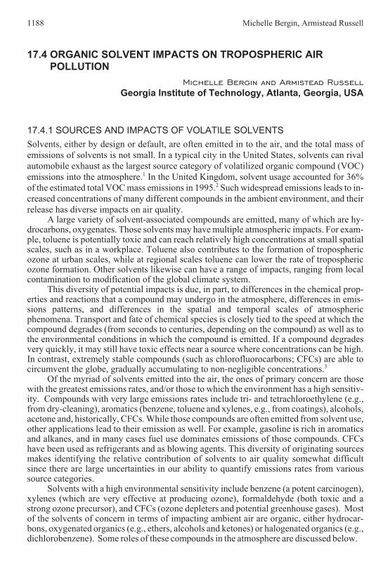
17.4 ORGANIC SOLVENT IMPACTS ON TROPOSPHERIC AIRPOLLUTION

Michelle Bergin and Armistead Russell

Georgia Institute of Technology, Atlanta, Georgia, USA

17.4.1 SOURCES AND IMPACTS OF VOLATILE SOLVENTS

Solvents, either by design or default, are often emitted in to the air, and the total mass of

emissions of solvents is not small. In a typical city in the United States, solvents can rival

automobile exhaust as the largest source category of volatilized organic compound (VOC)

emissions into the atmosphere.1 In the United Kingdom, solvent usage accounted for 36%

of the estimated total VOC mass emissions in 1995.2 Such widespread emissions leads to in-

creased concentrations of many different compounds in the ambient environment, and their

release has diverse impacts on air quality.A large variety of solvent-associated compounds are emitted, many of which are hy-

drocarbons, oxygenates. Those solvents may have multiple atmospheric impacts. For exam-ple, toluene is potentially toxic and can reach relatively high concentrations at small spatialscales, such as in a workplace. Toluene also contributes to the formation of troposphericozone at urban scales, while at regional scales toluene can lower the rate of troposphericozone formation. Other solvents likewise can have a range of impacts, ranging from localcontamination to modification of the global climate system.

This diversity of potential impacts is due, in part, to differences in the chemical prop-erties and reactions that a compound may undergo in the atmosphere, differences in emis-sions patterns, and differences in the spatial and temporal scales of atmosphericphenomena. Transport and fate of chemical species is closely tied to the speed at which thecompound degrades (from seconds to centuries, depending on the compound) as well as tothe environmental conditions in which the compound is emitted. If a compound degradesvery quickly, it may still have toxic effects near a source where concentrations can be high.In contrast, extremely stable compounds (such as chlorofluorocarbons; CFCs) are able tocircumvent the globe, gradually accumulating to non-negligible concentrations.3

Of the myriad of solvents emitted into the air, the ones of primary concern are thosewith the greatest emissions rates, and/or those to which the environment has a high sensitiv-ity. Compounds with very large emissions rates include tri- and tetrachloroethylene (e.g.,from dry-cleaning), aromatics (benzene, toluene and xylenes, e.g., from coatings), alcohols,acetone and, historically, CFCs. While those compounds are often emitted from solvent use,other applications lead to their emission as well. For example, gasoline is rich in aromaticsand alkanes, and in many cases fuel use dominates emissions of those compounds. CFCshave been used as refrigerants and as blowing agents. This diversity of originating sourcesmakes identifying the relative contribution of solvents to air quality somewhat difficultsince there are large uncertainties in our ability to quantify emissions rates from varioussource categories.

Solvents with a high environmental sensitivity include benzene (a potent carcinogen),xylenes (which are very effective at producing ozone), formaldehyde (both toxic and astrong ozone precursor), and CFCs (ozone depleters and potential greenhouse gases). Mostof the solvents of concern in terms of impacting ambient air are organic, either hydrocar-bons, oxygenated organics (e.g., ethers, alcohols and ketones) or halogenated organics (e.g.,dichlorobenzene). Some roles of these compounds in the atmosphere are discussed below.

1188 Michelle Bergin, Armistead Russell

While the toxicity of some solvents is uncertain, the role of emissions on direct expo-sure is not in question. Indoors, vaporized solvents can accumulate to levels of concern foracute and/or chronic exposure. However, the toxicity of solvents outdoors is not typically ofas great of concern as indoors except very near sources. Outdoors, solvents have adverse ef-fects other than toxicity. The importance of CFC emissions on stratospheric ozone, for ex-ample, is significant, but the problem is well understood and measures are in place toalleviate the problem. Reactive compounds can also aid in the formation of other pollutants,referred to as secondary pollutants because they are not emitted, but formed from directlyemitted primary precursors. Of particular concern is tropospheric ozone, a primary constitu-ent of photochemical smog. In the remainder of this chapter, the impacts of solvents on airquality are discussed, with particular attention given to the formation of tropospheric ozone.This emphasis is motivated by current regulatory importance as well as by lingering scien-tific issues regarding the role of volatile organics in secondary pollution formation.

17.4.2 MODES AND SCALES OF IMPACT

Many organic solvents are toxic, and direct exposure to the compound through the atmo-

sphere (e.g., via inhalation) can be harmful. While toxic effects of solvents rely on direct ex-

posure, many solvents also contribute to the formation of secondary pollutants such as

tropospheric ozone or particulate matter (PM), which cause health problems and damage

the environment on larger spatial scales such as over urban areas and multi-state/country re-

gions. Very slowly reacting solvent compounds also impact the atmosphere on the global

scale, which may cause imbalances in living systems and in the environment. While some

mechanisms of environmental imbalance are understood, the risks associated with global

atmospheric impacts are highly uncertain.Transport of solvents in the atmosphere is similar to most other gaseous pollutants,

and is dominated by the wind and turbulent diffusion. There is little difference between thetransport of different solvent compounds, and the fact that most solvents have much highermolecular weights than air does not lead to enhanced levels at the ground. Heavy solventsare, for the most part, as readily diffused as lighter solvents, although they may not vaporizeas fast. The higher levels of many solvents measured near the ground are due to proximity toemissions sources, which are near the surface, and the fact that most solvents degrade chem-ically as they mix upwards. A major difference in the evolution of various solvents is howfast they react chemically. Some, such as formaldehyde, have very short lifetimes whileothers, such as CFCs, last decades.

17.4.2.1 Direct exposure

Volatilization of solvents allows air to serve as a mode of direct exposure to many com-

pounds known to be toxic. Generally, direct exposure is a risk near strong or contained

sources, and can cause both acute and chronic responses. Most of the non-workplace expo-

sure to solvents occurs indoors. This is not surprising since, on average, people spend a vast

majority of their time indoors, and solvents are often used indoors. Outdoors, solvents rap-

idly disperse and can oxidize, leading to markedly lower levels than what is found indoors

near a source. For example, indoor formaldehyde levels are often orders of magnitude

greater than outdoors. There still are cases when outdoor exposure may be non-negligible,

such as if one spends a significant amount of time near a major source. Toxic effects of sol-

vents are fairly well understood, and many countries have developed regulatory structures

to protect people from direct exposure. The toxic effects of solvent emissions on ecosys-

tems are less well understood, but are of growing concern.

17.4 Organic solvent impacts on tropospheric air pollution 1189

17.4.2.2 Formation of secondary compounds

In addition to transport, organic compounds emitted into the air may also participate in com-

plex sets of chemical reactions. While many of these reactions “cleanse” the atmosphere

(most organic compounds ultimately react to form carbon dioxide), a number of undesirable

side effects may also occur. Such adverse impacts include the formation of respiratory irri-

tants and the destruction of protective components of the atmosphere. Ozone is a classic ex-

ample of the complexity of secondary atmospheric impacts. Ozone is a highly reactive

molecule consisting of three oxygen atoms (O3). In one part of the atmosphere ozone is ben-

eficial, in another, it is a pollutant of major concern. Solvents and other organic emissions

may either increase or decrease ozone concentrations, depending on the compound, loca-

tion of reaction, and background chemistry. The mechanisms of some adverse secondary re-

sponses are discussed below.

17.4.2.3 Spatial scales of secondary effects

Two layers of the Earth’s atmosphere are known to be adversely impacted by solvents - the

troposphere and the stratosphere. These two layers are closest to Earth, and have distinct

chemical and physical properties. The troposphere (our breathable atmosphere) is the clos-

est layer, extending from the Earth to a height of between 10 to 15 km. The rate of chemical

reaction generally determines the spatial scale over which emissions have an impact in the

troposphere. Most non-halogenated solvents have lifetimes of a week or less, and elevated

concentrations will only be found near the sources.4 Compounds that do not react rapidly in

the troposphere (e.g., CFCs) are relatively uniformly distributed, and may eventually reach

the stratosphere. The stratosphere is the next vertical layer of the atmosphere, extending

from the tropopause (the top of the troposphere) to about 50 km in altitude. Little vertical

mixing occurs in the stratosphere, and mixing between the troposphere and the stratosphere

is slow.Impacts on the stratosphere can be considered global in scale, while impacts on the

troposphere are generally urban or regional in scale. Distinct chemical systems of interestconcerning solvents in the atmosphere are stratospheric ozone depletion, global climatechange, and tropospheric photochemistry leading to enhanced production of ozone, particu-late matter, and other secondary pollutants such as organonitrates.

17.4.2.3.1 Global impacts

Because some solvent compounds are nearly inert, they can eventually reach the strato-

sphere where they participate in global scale atmospheric dynamics such as the destruction

of stratospheric ozone and unnatural forcing of the climate system. Stratospheric ozone de-

pletion by chlorofluorocarbons (CFCs) is a well-known example of global scale impacts.

CFCs were initially viewed as environmentally superior to organic solvents. They are gen-

erally less toxic than other similarly acting compounds, less flammable and are virtually in-

ert in the troposphere. Replacing solvents using volatile organic compounds (VOCs) with

CFCs was hoped to reduce the formation of tropospheric ozone and other secondary pollut-

ants. Because of their inert properties, there are no effective routes for the troposphere to re-

move CFCs, and, over the decades, emissions of CFCs have caused their accumulation,

enabling them to slowly leak into the stratosphere. In the stratosphere, the strong ultraviolet

(UV) light photodissociates CFCs, releasing chlorine, which then catalytically attacks

ozone. CFC use has been largely eliminated for that reason. Partially halogenated organic

solvents do not contribute as seriously to this problem since they react faster in the tropo-


sphere than CFCs, so the associated chlorine does not reach the stratosphere as efficiently.

CFCs and other solvent compounds also have a potential impact on global climate change.

17.4.2.3.2 Stratospheric ozone depletion

Natural concentrations of stratospheric O3 are balanced by the production of ozone via

photolysis of oxygen by strong UV light, and destruction by a number of pathways, includ-

ing reactions with nitrogen oxides and oxidized hydrogen products that are present.

Photolysis of an oxygen molecule leads to the production of two free oxygen atoms:

O2 + hν —> O + O [17.4.1]

Each oxygen atom can then combine with an oxygen molecule to form ozone:

O + O2 —> O3 [17.4.2]

Ozone is then destroyed when it reacts with some other compound, e.g., with NO:

O3 + NO —> NO2 + O2 [17.4.3]

Addition of either chlorine or bromine atoms leads to extra, and very efficient, path-ways for ozone destruction. The free chlorine (or bromine) atom reacts with ozone, and theproduct of that reaction removes a free oxygen atom:

Cl + O3 —> ClO + O2 [17.4.4]

ClO + O —> Cl + O2 [17.4.5]

Net (reactions 4+5 together): O3+ O —> 2 O2 [17.4.6]

Removing a free oxygen atoms also reduce ozone since one less ozone molecule willbe formed via reaction 17.4.2. Thus, the chlorine atom reactions effectively remove twoozone molecules by destroying one and preventing the formation of another. Additionally,the original chlorine atom is regenerated to catalytically destroy more ozone. This reactioncycle can proceed thousands of times, destroying up to 100,000 molecules of O3 before thechlorine is removed from the system (e.g., by the formation of HCl).

Reduction of ozone is greatly enhanced over the poles by a combination of extremelylow temperatures, decreased transport and mixing, and the presence of polar stratosphericclouds that provide heterogeneous chemical pathways for the regeneration of atomic chlo-rine. The resulting rate of O3 destruction is much greater than the rate at which it can be nat-urally replenished.

Current elevated levels of CFCs in the troposphere will provide a source of chlorine tothe stratosphere for decades, such that the recent actions taken to reduce CFC emissions(through the Montreal Protocol) will have a delayed impact.

17.4.2.3 Global climate forcing

Over the past decade, the potential for non-negligible changes in climate caused by human

activity has been an issue of great concern. Very large uncertainties are associated with both

estimations of possible effects on climate as well as estimations of the potential impacts of

changes in climate. However, current consensus in the international scientific community is

that observations suggest “a discernible human influence on global climate”.3


Solvent compounds, especially CFCs and their replacements, participate in climatechange as “greenhouse gases”. Greenhouse gases allow short-wave solar radiation to passthrough, much of which the earth absorbs and re-radiates as long-wave radiation. Green-house gases absorb the long-wave radiation, causing the atmosphere to heat up, thereby act-ing as a blanket to trap radiation that would normally vent back to space. Climate change is acontroversial and complex issue, but it is likely that restrictions such as those from theKyoto Protocol will be adopted for emissions of compounds strongly suspected of exacer-bating climate change. Many countries have already adopted stringent policies to reducegreenhouse gas emissions.

17.4.2.4 Urban and regional scales

Another area of concern regarding outdoor air is exposure to secondary pollutants that are

due, in part, to chemical reactions involving solvent compounds. Examples include the for-

mation of elevated levels of ozone, formaldehyde, organonitrates, and particulate matter.

Formaldehyde, a suspected carcinogen, is an oxidation product of organic compounds. Tro-

pospheric ozone and organonitrates, as discussed below, are formed from a series of reac-

tions of organic gases and nitrogen oxides in the presence of sunlight. Particulate matter

formation is linked to ozone, and some solvents may react to form particulate matter. The

particulate matter of concern is small (generally less than 2.5 µm in diameter) usually

formed by gas-to-aerosol condensation of compounds via atmospheric chemical reactions.

Ozone and particulate matter are both regulated as “criteria” pollutants in the United States

because they have been identified as risks to human health. Ozone is believed to cause respi-

ratory problems and trigger asthma attacks, and PM has a variety of suspected adverse

health outcomes (e.g., respiratory and coronary stress and failure). Many organonitrates,

such as peroxyacetyl nitrate, are eye irritants and phytotoxins. Currently, the formation and

effects of ozone are better understood than those of fine particulate matter and

organonitrates. The following section of this chapter discusses the effects, formation, and

control of tropospheric ozone. The role of solvents in forming particulate matter is currently

viewed as less urgent.

17.4.3 TROPOSPHERIC OZONE

Tropospheric ozone, a primary constituent of photochemical smog, is naturally present at

concentrations on the order of 20-40 parts per billion (ppb).4 However, elevated levels of

ground-level ozone are now found virtually worldwide, reaching in some cities concentra-

tions of up to 10 times the natural background.

17.4.3.1 Effects

Ozone is believed to be responsible for both acute (short-term) and chronic (long-term) im-

pacts on human health, especially on lung functions. Major acute effects of ozone are de-

creased lung function and increased susceptibility to respiratory problems such as asthma

attacks and pulmonary infection. Short-term exposure can also cause eye irritation, cough-

ing, and breathing discomfort.5-7 Evidence of acute effects of ozone is believed to be “clear

and compelling”.8 Chronic health effects may present a potentially far more serious prob-

lem; however, definitive evidence is difficult to obtain. Recent studies do suggest that ambi-

ent levels of ozone induce inflammation in human lungs, which is generally accepted as a

precursor to irreversible lung damage,6 and chronic animal exposure studies at concentra-

tions within current ambient peak levels indicate progressive and persistent lung function

and structural abnormalities.5,8


Crop damage caused by air pollution has also received much attention. It is estimated that

10% to 35% of the world’s grain production occurs in regions where ozone pollution likely

reduces crop yields.9 Air pollution accounts for an estimated several billion dollar crop loss

every year in the United States alone, and research and analysis suggests that about 90% of

this crop loss can be directly or indirectly attributed to ozone.10 Evidence also indicates that

ozone may cause short- and long-term damage to the growth of forest trees,11 as well as al-

tering the biogenic hydrocarbon emissions of vegetation.12

17.4.3.2 Tropospheric photochemistry and ozone formation

In the lowest part of the atmosphere, chemical interactions are very complex. A large num-

ber of chemical compounds are present, the levels of many of these compounds are greatly

elevated, and emissions vary rapidly due to both natural and anthropogenic sources. Ozone

formation in the troposphere results from non-linear interactions between NOx, VOCs, and

sunlight.4,13 In remote regions, ozone formation is driven essentially by methane,14 however

elsewhere most VOCs participate in ozone generation. For example, measurements of

non-methane organic compounds in the South Coast Air Basin of California during the

1987 Southern California Air Quality Study, identified more than 280 ambient hydrocarbon

and oxygenated organic species,15 many of which originated from solvents and contribute in

differing degrees to ozone generation.

The only significant process forming O3 in the lower atmosphere is the photolysis of NO2

(reaction with sunlight), followed by the rapid reactions of the oxygen atoms formed with

O2.The only significant process forming O3 in the lower atmosphere is the photolysis of

NO2 (reaction with sunlight), followed by the rapid reactions of the oxygen atoms formedwith O2.

NO2 + hν → O(3P) + NO [17.4.7]

O(3P) + O2 + M → O3 + M

This is reversed by the rapid reaction of O3 with NO,

O3 + NO → NO + O2 [17.4.8]

This reaction cycle results in a photostationary state for O3, where concentrations onlydepend on the amount of sunlight available, dictated by the NO2 photolysis rate (k1) and the[NO2]/[NO] concentration ratio.

[ ] [ ][ ]

Ok NO

k NOsteady state3

1 2

2−

= [17.4.9]

Because of this photostationary state, ozone levels generally rise and fall with the sun,behavior that is referred to as “diurnal.”

If the above NOx cycle were the only chemical process at work, the steady-state con-centrations of ozone would be relatively low. However, when VOCs such as organic solventcompounds are present, they react to form radicals that may either (1) consume NO or (2)convert NO to NO2. This additional reaction cycle combined with the above photostationarystate relationship causes O3 to increase.


Although many types of reactions are involved,4,13,16,17 the major processes for mostVOCs can be summarized as follows:

VOC + OH → RO2 + products [17.4.10a]

RO2 + NO → NO2 + radicals [17.4.10b]

radicals → ...→ OH + products [17.4.10c]

products → ...→...+ CO2 [17.4.10d]

The last two pseudo-reactions given comprise many steps, and the products often in-clude formaldehyde, carbon monoxide and organonitrates. The rate of ozone increasecaused by these processes depends on the amount of VOCs present, the type of VOCs pres-ent, and the level of OH radicals and other species with which the VOCs can react. One ofthe major determinants of a compound’s impact on ozone is the rate of the reaction of theparticular VOC with the hydroxyl radical via reaction [17.4.10a], above. The total amountof ozone formed is largely determined by the amount of VOC and NOx available.

The dependence of O3 production on the initial amounts of VOC and NOx is frequentlyrepresented by means of an ozone isopleth diagram. An example of such a diagram isshown in Figure 17.4.1. The diagram is a contour plot of ozone maxima obtained from alarge number of air quality model simulations using an atmospheric chemical mechanism.Initial concentrations of VOC and NOx are varied; all other variables are held constant. No-tice that there is a “ridge” along a certain VOC-to-NOx ratio where the highest ozone con-centrations occur at given VOC levels. This is referred to as the “optimum” VOC-to-NOx

ratio. While the atmosphere is more complicated than this idealized system, important fea-tures are very similar.

VOC-to-NOx ratios sufficiently low to retard ozone formation from an optimum ratio(represented in the upper left quadrant of Figure 17.4.1) can occur in central cities and inplumes immediately downwind of strong NOx sources. Rural environments tend to be char-acterized by fairly high VOC-to-NOx ratios because of the relatively rapid removal of NOx


Figure 17.4.1. Ozone isopleth diagram showing the dependencies of ozone on varying levels of initial VOCs and

NOx. Concentrations are given in ppb. [Adapted from M.S. Bergin et al., Enc. of Env. Analysis and Remediation,

29, 3029, (1998)]

from non-local sources as compared to that of VOCs, coupled with the usual absence ofstrong local NOx sources and the presence of natural VOC sources. In such rural environ-ments, the formation of ozone is limited more by the absence emissions of NOx, and mostozone present was directly transported from upwind. Indeed, in most of the troposphere,except in areas of strong NOx sources, the availability of NOx governs ozone production.

17.4.3.3 Assessing solvent impacts on ozone and VOC reactivity

As mentioned previously, the contribution of solvents to the VOC levels, and hence ozone

formation, is significant. For example, in Los Angeles, about 25% of the VOC mass is from

solvent use.1 This fraction is down from earlier years due to various controls such as using

water-based paints and enclosing/controlling paint spraying operations. On the other hand,

reduction in the use of CFCs as propellants has led to an increase in organic emissions from

substituted compounds.2 However, the impact on ozone formation by a specific source is

not directly proportional to the amount of VOC emitted by that source. A major determinant

of the ozone forming potential is the reactivity of the compound or compound mixture emit-

ted. Reactivity can be viewed as the propensity for a compound to form ozone, and this pro-

pensity varies dramatically between compounds and between environments.18,19

As seen in Table 17.4.1, ‘box’ model (single cell) simulations designed to representsummertime conditions in Los Angeles, California indicate that the amount of carbon asso-ciated with each class of compound only roughly corresponds to the amount of ozoneformed from those compounds. Methane, which reacts very slowly but comprises most ofthe carbon, contributes little to ozone formation. Alkenes and aromatics are only a smallpart of the total carbon, but lead to much of the ozone formation.

Table 17.4.1. Percentage of ozone production attributable to each organic. Thepercentages shown should be viewed as only approximate, and will depend uponlocal emissions characteristics. (*While not considered organic carbon, carbonmonoxide acts to facilitate ozone formation similar to organic compounds.) [Adaptedfrom F.M. Bowman and J.H. Seinfeld, J. Geophys. Res., 99, 5309, (1994) and M.S.Bergin et al., Env. Sci. Technol., 29, 3029 (1998)]

Compound ClassPercent of carbon in each

specified class

Percent of ozone due to

specified organic class

carbon monoxide* 35 6

methane 40 1

aldehydes and ketones 1 3

non-methane alkanes, ~4C 8 17

non-methane alkanes, ~8C 5 16

aromatics, including toluene 3 5

aromatics, including xylenes

and others3 13

ethene 2 12

biogenic alkenes ans isoprene 1 10

other alkenes 2 17


17.4.3.3.1 Quantification of solvent emissions on ozone formation

Two methods are generally employed to quantify the role pollutants play in forming ozone:

experimental and computational. Both types of estimation approaches have their limita-

tions. In the case of physical experiments, it is difficult to fully simulate ambient conditions,

so the results do not have general applicability. In the case of computational approaches, un-

certainties and approximations in the model for airshed conditions, in its formulation, and in

the chemical mechanism cause uncertainties in the predicted ozone impacts. For these rea-

sons, modeling predictions and experimental measurements are used together.

17.4.3.3.1.1 Experimental analysis

Experimental analysis is performed using environmental ‘smog’ chambers, either with a se-

ries of single hydrocarbons irradiated in the presence of NOx or using complex mixtures to

simulate, for example, automobile exhaust emitted into characteristic urban ambient condi-

tions. Such chambers are large reaction vessels (some with internal volumes of cubic me-

ters), in which air and small amounts of hydrocarbons and NOx are injected, and then

irradiated with real or artificial light. Both indoor and outdoor chambers are used so behav-

iors can be evaluated under natural radiative conditions and under controlled conditions.

While these experiments18-23 clearly indicate differences in ozone formation from individual

hydrocarbons, they do not represent some important physical systems of urban pollution

such as the mixing processes and continuing emissions cycles. Such experiments have fo-

cused both on groups of compounds as well as specific VOCs, including solvents. A partic-

ular limitation has been studying very low vapor pressure solvents because it is difficult to

get enough of the compound into the vapor phase in the chamber to appreciably change the

ozone levels. Another limitation is the expense of using smog chambers to simulate a large

range of conditions that might occur in the atmosphere. On the other hand, smog chambers

are very powerful, if not fundamental, for developing chemical mechanisms that describe

the reaction pathways that can be used in computational approaches.

17.4.3.3.1.2 Computational analysis (air quality models)

Given the limitations of physical experiments to simulate atmospheric conditions, computer

models have been developed to assess the impact of emissions on ozone. These models,

called airshed models, are computerized representations of the atmospheric processes re-

sponsible for air pollution, and are core to air quality management.23 They have been ap-

plied in two fashions to assess how solvents affect ozone. One approach is to conduct a

number of simulations with varying levels of solvent emissions.2 The second approach is to

evaluate individual compounds and then calculate the incremental reactivity of solvent mix-

tures.19,21,24-28

Derwent and Pearson2 examined the impact of solvent emissions on ozone by simulat-ing air parcel trajectories ending in the United Kingdom and perturbing the emissions to ac-count for an anticipated 30% mass reduction in VOCs from solvents between 1995 and2007. They found a small decrease in ozone-from 78 to 77 ppb in the mean peak ozone inthe UK, and a 9 ppb reduction from 129 ppb outside of London. A more substantial decreaseof 33 ppb from the 129 ppb peak outside of London was found from reducing non-solventmass VOC emissions by 30% outside of the UK and 40% within the UK. This suggests thatthe VOC emissions from sources other than solvents have a higher average reactivity, as isdiscussed by McBride et al.29

While the types of simulations conducted by Derwent and Pearson2 are important tounderstanding the net effect of solvent emissions on ozone, there is an unanswered associ-ated and important question, that being which specific solvents have the greatest impacts.


This question is critical to assessing if one solvent leads to significantly more ozone forma-tion than a viable substitute (or vice versa).

To evaluate the contribution of individual organic compounds to ozone formation, theuse of incremental reactivities (IR) was proposed,18-21 defined as the change in ozone causedby a change in the emissions of a VOC in an air pollution episode. To remove the depend-ence on the amount of VOC added, incremental reactivity is defined by equation [17.4.11]as the limit as the amount of VOC added approaches zero, i.e., as the derivative of ozonewith respect to VOC:

[ ][ ]

IRO

VOCi

i

=∂

∂3

[17.4.11]

Here, IRi is the incremental reactivity and the subscript i denotes the VOC being examined.

This definition takes into account the effects of all aspects of the organic’s reaction mecha-

nism and the effects of the environment where the VOC is emitted. A similar quantity is the

relative reactivity,23 RRi:

RRR

F Ri

i

B i

i

N

i

=

=∑

1

[17.4.12]

where:

FB imass fraction of compound i in the reference mixture

IRi incremental reactivity of species i (grams ozone formed per gram compound i emitted)

In this case, the incremental reactivity is normalized by the reactivities of a suite oforganics, thus removing much of the environmental dependencies found when using IRsdefined by [17.4.11]. This metric provides a means for directly comparing individual com-pounds to each other in terms of their likely impact on ozone.

A number of investigators have performed calculations to quantify incremental and/orrelative reactivities for various solvents and other organics23-28,30 and references therein.Those studies found very similar results for the relative reactivities of most compoundsfound in solvents. Figure 17.4.2 (based on references 23, 24 and 26) shows the relative reac-tivities for some of the more common compounds, as well as possible solvent substitutesand isoprene, a naturally emitted organic. (For a more extensive list of relative reactivities,see 19, 27 and 30.) As can be seen, even normalized compound reactivities can vary by or-ders of magnitude. Some compounds even exhibit “negative” reactivities, that is that theiremission can lead to ozone decreases under specific conditions. In particular, negative reac-tivities are found most commonly when the levels of NOx are low, e.g., in non-urban loca-tions. For example, Kahn et al.,26 found that a solvent can promote ozone formation in onearea (e.g., near downtown Los Angeles), but retard ozone formation further downwind.Kahn also found that the relative reactivities of the eight different solvents studied weresimilar in very different locations, e.g., Los Angeles, Switzerland and Mexico City.

Looking at Figure 17.4.2, it is apparent that alkenes and aromatic hydrocarbons withmultiple alkyl substitutions (e.g., xylenes and tri-methyl benzene) have relatively high reac-tivities. Alcohols, ethers and alkanes have lower reactivities. Halogenated organics havesome of the lowest reactivities, so low that they are often considered unreactive. This sug-gests that there are two ways to mitigate how solvents contribute to air quality problems.The more traditional method is to reduce the mass of organic solvent emissions (e.g., by us-ing water-based paints). A second approach is to reduce the overall reactivity of the solvent


used, e.g., by switching to ethers, alcohols, alkanes or halogenated compounds. Solventsubstitution, however, is complicated by the need to maintain product quality.

17.4.4 REGULATORY APPROACHES TO OZONE CONTROL ANDSOLVENTS

Historically, regulatory approaches to reducing ozone concentrations have relied reducing

the mass emissions of VOCs,2,4 and this has led to stringent controls on solvents. Two fac-

tors are important in determining if an organic solvent is considered a VOC: its reactivity

(discussed above) and its vapor pressure. In the U.S., traditionally, if a compound was less

reactive than ethane, it was considered unreactive. Such compounds include many

halogenated species and some acetates and ethers. Recently, acetone was also added as an

unreactive compound. A vapor pressure threshold is also used in many areas (e.g., Europe)

since it is viewed that compounds with very low vapor pressures will not be emitted rapidly

into the atmosphere. It has been argued that a vapor pressure limit may not be appropriate

since, given time, even lower vapor pressure compounds will have ample time to evaporate.

Just recently, California is considering regulations that more fully account for the full range

of reactivities that solvents possess. This is due, in part, to make it easier for manufacturers

to meet stringent regulations being adopted in that state to help them meet their air quality

goals. It is likely that other areas will also have to employ increasingly more stringent regu-

lations, to both lower ozone and alleviate other environmental damage.In many countries, greater focus is now being placed on reducing NOx emissions to

mitigate ozone formation. This has important ramifications for solvent use, indicating the


Figure 17.4.2. Solvent relative reactivities based on mass of ozone formed per gram of solvent emitted into the gas

phase. PCBTF is para-chlorobenzo-trifluoride, BTF is benzo-trifluoride and TBA is tertiary butyl acetate.

[Adapted from M.S. Bergin et al., Env. Sci. Technol., 29, 3029 (1998) and M. Khan et al., Atmos. Env., 33, 1085

(1999)].

regulatory focus is now turning from VOCs towards NOx, the other main precursor toozone. Another imminent regulatory issue is the control of ambient fine particulate matter.While the role of solvent emissions in forming particulate matter is not well understood,studies to date do not suggest they are a major contributor.

17.4.5 SUMMARY

Solvents are, and will continue to be, one of the major classes of organic compounds emit-

ted into the atmosphere. These compounds have a wide range of air quality impacts. Accu-

mulation of toxic compounds indoors is of concern, although outdoors the concern of

toxicity is significantly less substantial due to rapid dilution. In the stratosphere, some of the

halogenated solvents lead to depletion of the protective layer of ozone, while in the tropo-

sphere solvents generally lead to increased ozone levels, where it adversely affects health

and the environment. The former has led to regulations of CFCs, and the latter to regulations

of organic solvents. Some solvents are also considered to be precursors to the formation of

secondary tropospheric pollutants other than ozone, such as particulate matter, however

these relationships are currently less certain.

In the aggregate, total VOC emissions from solvents in the U.S. are the second largest single

source category in polluted urban areas, falling just behind motor vehicle VOC emissions

both in terms of mass and urban ozone production. For now, regulations are designed to re-

duce the loss of ozone in the stratosphere and the formation of excess ozone in the tropo-

sphere. However, while some solvents are very reactive, others are substantially less

reactive, suggesting that there is considerable opportunity to reduce urban ozone formation

from solvents by utilizing substitutes with low ozone forming potentials. Currently, most

regulations are targeted at reducing the mass of VOC emissions, not their relative impacts

on ozone.

REFERENCES

1 SCAQMD (South Coast Air Quality Management District). (1996). 1997 Air Quality Management Plan.

November.

2 R.G. Derwent and J.K. Pearson, Environ. Technol., 18, 1029 (1997).

3 Climate Change 1995: The Science of Climate Change. Contribution of Working Group I to the Second

Assessment Report of the Intergovernmental Panel on Climate Change (IPCC). Ed. J.T. Houghton, et al.

Cambridge University Press, Cambridge, Great Britain. 1996.

4 NRC (National Research Council). Rethinking the Ozone Problem in Urban and Regional Air Pollution.

National Academy Press, Washington, DC. (1991).

5 OTA (U.S. Congress, Office of Technology Assessment). Catching Our Breath: Next Steps for Reducing

Urban Ozone, OTA-O-412, U.S. Government Printing Office, Washington, DC. July,1989.

6 S.M. Horvath and D.J.McKee (1994). In D.J. McKee, ed., Tropospheric Ozone: Human Health and

Agricultural Impacts, CRC Press/Lewis Publishers, Boca Raton, FL, Chapter 3.

7 M. Lippmann, Environ. Sci. & Technol., 25(12), 1954, (1991).

8 M. Lippmann, J. of Exposure Analysis and Environmental Epidemiology, 3(1), 103, (1993).

9 W.L.Chameides, P.S. Kasibhatla, J Yienger, and H. Levy II., Science, 264(5155), 74, (1994).

10 D.T. Tingey, D.M. Olszyk, A.A.Herstrom, and E.H. Lee, (1994). “Effects of Ozone on Crops” in

D.J. McKee, ed., Tropospheric Ozone: Human Health and Agricultural Impacts, CRC Press/Lewis

Publishers, Boca Raton, FL, Chapter 6.

11 S.B.McLaughlin and L.J. Downing, Nature, 374(6519), 252, (1995).

12 W. Mehlhorn, Nature, 327, 417, (1989).

13 J.H. Seinfeld and S.N. Pandis, Atmospheric Chemistry and Physic: From Air Pollution to Climate

Change, New York: J. Wiley & Sons, (1998).

14 J.A. Logan, M.J. Pather, S.C. Wofsy, and M.B. McElroy, J. Geophys. Res., 86, 7210, (1981).

15 F.W.Lurmann and H.H. Main, Analysis of the Ambient VOC Data Collected in the Southern California Air

Quality Study, final report, Contract A832-130, California Air Resources Board, Sacramento, CA., 1992.

16 R. Atkinson, Atmos. Environ., 24A, 1, (1990).


17 R. Atkinson, J. Phys. Chem. Ref. Data, Monograph No. 2, (1994).

18 W.P.L. Carter, Atmos. Environ., 24A, 481, (1990).

19 W.P.L.Carter, (1991). Development of Ozone Reactivity Scales for Volatile Organic Compounds,

EPA 600/3-91-050. U.S. Environmental Protection Agency, Research Triangle Park, NC (August).

20 W.P.L. Carter and R. Atkinson, Environ. Sci. and Technol., 23, 864, (1989).

21 W.P.L. Carter, Atmos. Environ., 29, 2513, (1995).

22 N.A. Kelly and P. Wang, (1996) Part I: Indoor Smog Chamber Study of Reactivity in Kelly, N.A.; Wang, P.;

Japar, S.M.; Hurley, M.D.; and Wallington, T.J. (1996). Measurement of the Atmosphere Reactivity of

Emissions from Gasoline and Alternative-Fueled Vehicles: Assessment of Available Methodologies,

Second-Year Final Report, CRC Contract No. AQ-6-1-92 and NREL Contract No. AF-2-112961.

Environmental Research Consortium, (September).

23 M.S. Bergin, A.G. Russell, W.P.L. Carter, B.E. Croes, and J.H. Seinfeld, Ozone Control and VOC

Reactivity, in the Encyclopedia of Environmental Analysis and Remediation, Ed. R.A. Meyers, J. Wiley

& Sons, Inc, New York, NY. 1998.

24 M.S. Bergin et al., Env. Sci Technol., 29, 3029 (1998)

25 F.M. Bowman and J.H. Seinfeld, J. Geophys. Res., 99, 5309, (1994a).

26 M. Khan et al., Atmos. Env., 33, 1085 (1999).

27 W.P.L. Carter, J. Air and Waste Mgmt. Assoc., 44, 881, (1994a).

28 R.G. Derwent, and M.E. Jenkin, Atmos. Environ., 25(A):1661-1673 (1991).

29 S. B. McBride et al., Env. Sci. Technol., 31, 238a, (1997)

30 http://www.cert.ucr.edu/~carter/bycarter.htm


Documents

Environmental Impact of Solvents - mdmasearch.mdma.ch/picproxie_docs/000532906-14581_17.pdf · Environmental Impact of Solvents 17.1 THE ENVIRONMENTAL FATE AND MOVEMENT OF ORGANIC