Environmental & Engineering Geoscience

Environmental &Engineering GeoscienceFEBRUARY 2015 VOLUME XXI, NUMBER 1

THE JOINT PUBLICATION OF THE

ASSOCIATION OF ENVIRONMENTAL AND ENGINEERING GEOLOGISTS

AND THE GEOLOGICAL SOCIETY OF AMERICA

SERVING PROFESSIONALS IN

ENGINEERING GEOLOGY, ENVIRONMENTAL GEOLOGY, AND HYDROGEOLOGY

Environmental & Engineering Geoscience (ISSN 1078-7275) is pub-lished quarterly by the Association of Environmental and EngineeringGeologists (AEG) and the Geological Society of America (GSA).Periodicals postage paid at AEG, 1100 Brandywine Blvd, Suite H, Zane-sville, OH 43701-7303 and additional mailing offices.

EDITORIAL OFFICE: Environmental & EngineeringGeoscience journal, Department of Geology, Kent StateUniversity, Kent, OH 44242, U.S.A. phone: 330-672-2968, fax:330-672-7949, [email protected].

CLAIMS: Claims for damaged or not received issues will behonored for 6 months from date of publication. AEG membersshould contact AEG, 1100 Brandywine Blvd, Suite H, Zanes-

. GSA members who are not members ofAEG should contact the GSA Member Service center. Allclaims must be submitted in writing.

POSTMASTER: Send address changes to AEG, 1100 Brand- ywine Blvd, Suite H, Zanesville, OH 43701-7303 . Include both oldand new addresses, with ZIP code. Canada agreement numberPM40063731. Return undeliverable Canadian addresses toStation A P.O. Box 54, Windsor, ON N9A 6J5 Email: [email protected].

DISCLAIMER NOTICE: Authors alone are responsible forviews expressed in articles. Advertisers and their agencies aresolely responsible for the content of all advertisements printed andalso assume responsibility for any claims arising therefromagainst the publisher. AEG and Environmental & EngineeringGeoscience reserve the right to reject any advertising copy.

SUBSCRIPTIONS:

Member subscriptions: AEG members automatically receive the journal as part of their AEG membership dues. Additionalsubscriptions may be ordered at $40 per year. GSA memberswho are not members of AEG may order for $40 per year ontheir annual GSA dues statement or by contacting GSA.

Nonmember subscriptions are $175 and may be ordered fromthe subscription department of either organization. A postagedifferential of $10 may apply to nonmember subscribers outsidethe United States, Canada, and Pan America. Contact AEG at844-331-7867; contact GSA Subscription Services, c/oAmerican Institute of Physics, 2 Huntington Quadrangle, Suite1N01, Melville, NY 11747-4502.

Single copies are $50.00 each. Requests for single copies shouldbe sent to AEG, 1100 Brandywine Blvd, Suite H, Zanesville, OH

© 2015 by the Association of Environmental & EngineeringGeologists

All rights reserved. No part of this publication may be reproduced or transmitted in any form or by any means, electronic or mechanical, including photocopying, recording, orby any information storage and retrieval system, without permission in writing from AEG.

THIS PUBLICATION IS PRINTED ON ACID-FREE PAPER

ABDUL SHAKOOR

Department of GeologyKent State University

Kent, OH 44242330-672-2968

[email protected]

BRIAN G. KATZ

Florida Department of EnvironmentalProtection

2600 Blair Stone Rd.Tallahassee, FL 32399

[email protected]

EDITORS Cover photo

Cal Trans employee on California Route 2, within the San Gabriel Mountainsnorth of Los Angeles, CA, September 17, 2006, during the Station Fire. Dryravel is actively forming a debris cone encroaching on the traffic lane. Dust risesas sand-sized particles to rocks nearly a foot in diameter cascade from the steepslope. Photo Credit: U.S. Forest Service, Burned Area Emergency Response(BAER) Team geologist, Jonathan Swartz.

SUBMISSION OF MANUSCRIPTS

Environmental & Engineering Geoscience (E&EG), is a quar-terly journal devoted to the publication of original papers thatare of potential interest to hydrogeologists, environmental andengineering geologists, and geological engineers working in siteselection, feasibility studies, investigations, design or construc-tion of civil engineering projects or in waste management,groundwater, and related environmental fields. All papers arepeer reviewed.

The editors invite contributions concerning all aspects of envi-ronmental and engineering geology and related disciplines.Recent abstracts can be viewed under “Archive” at the website, “http://eeg.geoscienceworld.org”. Articles that report onresearch, case histories and new methods, and book reviewsare welcome. Discussion papers, which are critiques of print-ed articles and are technical in nature, may be published withreplies from the original author(s). Discussion papers andreplies should be concise.

To submit a manuscript go to http://eeg.allentrack.net. If youhave not used the system before, follow the link at the bottom ofthe page that says New users should register for an account.Choose your own login and password. Further instructions willbe available upon logging into the system. Please carefully readthe “Instructions for Authors”.

Authors do not pay any charge for color figures that are essen-tial to the manuscript. Manuscripts of fewer than 10 pages maybe published as Technical Notes.

For further information, you may contact Dr. Abdul Shakoor atthe editorial office.

JOHN W. BELL

Nevada Bureau of Mines andGeologyRICHARD E. JACKSON

(Book Reviews Editor)Geofirma Engineering, Ltd.JEFFREY R. KEATON

AMEC AmericasPAUL G. MARINOS

National Technical Universityof Athens, Greece

JUNE E. MIRECKI

U.S. Army Corps of Engineers

PETER PEHME

Waterloo Geophysics, IncNICHOLAS PINTER

Southern Illinois University

PAUL M. SANTI

Colorado School of MinesROBERT L. SCHUSTER

U.S. Geological SurveyROY J. SHLEMON

R. J. Shlemon& Associates, Inc.

GREG M. STOCK

National Park ServiceRESAT ULUSAY

Hacettepe University, TurkeyCHESTER F. “SKIP” WATTS

Radford UniversityTERRY R. WEST

Purdue University

EDITORIAL BOARD

ASSOCIATE EDITORS

JEROME V. DEGRAFF

USDA Forest ServiceTHOMAS J. BURBEY

Virginia Polytechnic InstituteSYED E. HASAN

University of Missouri, Kansas City

ROBERT H. SYDNOR

ConsulantCHESTER F. WATTS (SKIP)Radford University

43701-7303.

ville, OH 43701-7303

Environmental &Engineering Geoscience

Volume 21, Number 1, February 2015

Table of Contents

1 Simulations of Potential Future Conditions in the Cache Critical Groundwater Area, Arkansas

Haveen M. Rashid, Brian R. Clark, Hanan H. Mahdi, Hanadi S. Rifai, and Haydar J. Al-Shukri

21 Uncertainty Associated with Evaluating Rockfall Hazard to Roads in Burned AreasJerome V. De Graff, Bill Shelmerdine, Alan Gallegos, and David Annis

35 Complex Landslide Triggered in an Eocene Volcanic-Volcaniclastic Succession along Sutherland River,

British Columbia, Canada

Andree Blais-Stevens, Marten Geertsema, James W. Schwab, and Theo W. J. Van Asch

47 Modeling the Northern Coastline of Yucatan, Mexico, with GENESIS

Roger Gonzalez-Herrera, Alfonso Solıs-Pimentel, Carlos Zetina-Moguel, and Ismael Marino-Tapia

63 Collection and Application of Outcrop Measurements in Glacial Materials for Geo-Engineering and

Hydrogeology along the Vermilion River, East-Central Illinois

Christopher J. Stohr, Andrew J. Stumpf, and Barbara J. Stiff

Simulations of Potential Future Conditions in the

Cache Critical Groundwater Area, Arkansas

HAVEEN M. RASHID

Dams and Water Resources Department, Faculty of Engineering, University ofSulaimani, Sulaymaniyah, Iraq; and Department of Applied Science, University of

Arkansas, 2801 South University Avenue, Little Rock, AR 72204

BRIAN R. CLARK

U.S. Geological Survey, Arkansas Water Science Center, Fayetteville Field Office,700 West Research Boulevard, MS 36, Fayetteville, AR 72701

HANAN H. MAHDI

Graduate Institute of Technology, University of Arkansas,2801 South University Avenue, Little Rock, AR 72204

HANADI S. RIFAI

Civil and Environmental Engineering Department, University of Houston,Room N107, Engineering Building 1, Houston, TX 77204-4003

HAYDAR J. AL-SHUKRI

Department of Applied Science, University of Arkansas,2801 South University Avenue, Little Rock, AR 72204

Key Terms: Modeling, Aquifer, Calibration, Pilot Point,MODFLOW

ABSTRACT

A three-dimensional finite-difference model for partof the Mississippi River Valley alluvial aquifer in theCache Critical Groundwater Area of eastern Arkansaswas constructed to simulate potential future conditionsof groundwater flow. The objectives of this study wereto test different pilot point distributions to findreasonable estimates of aquifer properties for thealluvial aquifer, to simulate flux from rivers, and todemonstrate how changes in pumping rates for differentscenarios affect areas of long-term water-level declinesover time. The model was calibrated using theparameter estimation code. Additional calibration wasachieved using pilot points with regularization andsingular value decomposition. Pilot point parametervalues were estimated at a number of discrete locationsin the study area to obtain reasonable estimates ofaquifer properties. Nine pumping scenarios for theyears 2011 to 2020 were tested and compared to thesimulated water-level heads from 2010. Hydraulicconductivity values from pilot point calibration rangedbetween 42 and 173 m/d. Specific yield values ranged

between 0.19 and 0.337. Recharge rates ranged between0.00009 and 0.0006 m/d. The model was calibratedusing 2,322 hydraulic head measurements for the years2000 to 2010 from 150 observation wells located in thestudy area. For all scenarios, the volume of waterdepleted ranged between 5.7 and 23.3 percent, except inScenario 2 (minimum pumping rates), in which thevolume increased by 2.5 percent.

INTRODUCTION

The Mississippi River Valley alluvial aquifer, oftentermed the ‘‘alluvial aquifer,’’ is a water-bearingassemblage consisting of gravels and sands thatunderlies about 82,879 km2 of Missouri, Kentucky,Tennessee, Mississippi, Louisiana, and Arkansas(Czarnecki et al., 2002). In eastern Arkansas, thealluvial aquifer occurs in an area generally 80 to 201 kmwide by about 402 km long adjacent to the MississippiRiver (Czarnecki et al., 2002). Crowley’s Ridge, whichtrends approximately north to south in northeasternArkansas, separates the alluvial aquifer into two parts.The ridge rises 30 to 76 m above the surroundingalluvial plain, is about 241 km in length, and averagesabout 4.8 km wide in the southern half and 16 km widein the northern half (Gonthier and Mahon, 1993).

Environmental & Engineering Geoscience, Vol. XXI, No. 1, February 2015, pp. 1–19 1

Pumping of groundwater from the alluvial aquiferfor agriculture started in the early 1900s in theGrand Prairie area for the irrigation of rice andsoybeans. The first documentation of water-leveldeclines in the alluvial aquifer was in 1927 (Engler etal., 1945; Czarnecki, 2010). Long-term water-levelmeasurements in the alluvial aquifer show an averageannual decline of 0.3 m/yr in some areas (Freiwald,2005; Schrader, 2010). Because of the heavy demandsplaced on the aquifer for irrigation, two major conesof depression have formed in the potentiometric

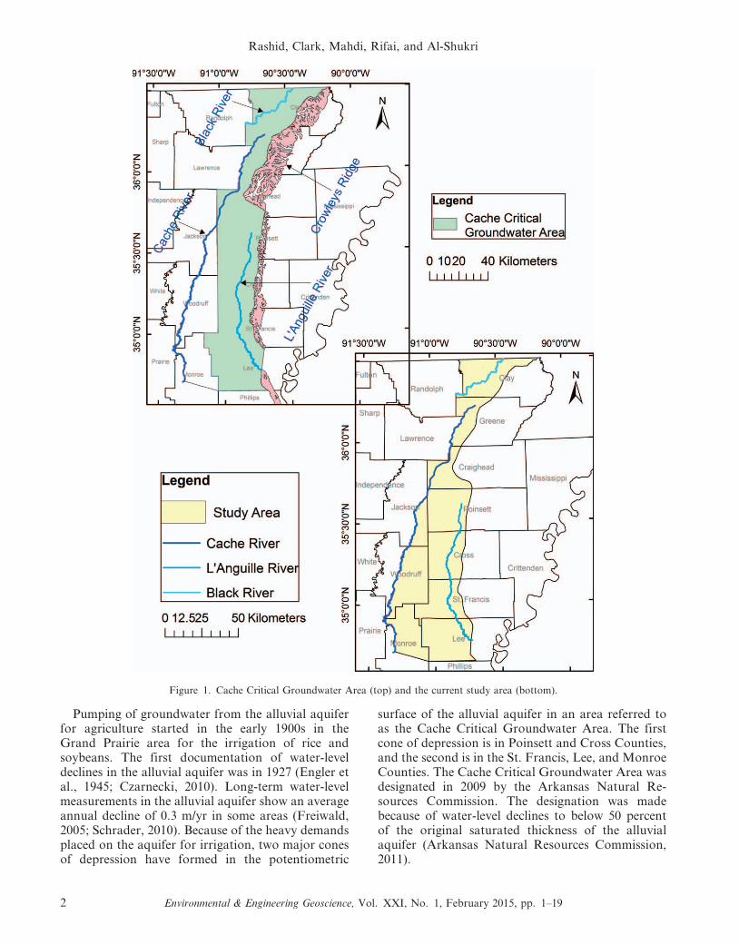
surface of the alluvial aquifer in an area referred toas the Cache Critical Groundwater Area. The firstcone of depression is in Poinsett and Cross Counties,and the second is in the St. Francis, Lee, and MonroeCounties. The Cache Critical Groundwater Area wasdesignated in 2009 by the Arkansas Natural Re-sources Commission. The designation was madebecause of water-level declines to below 50 percentof the original saturated thickness of the alluvialaquifer (Arkansas Natural Resources Commission,2011).

Figure 1. Cache Critical Groundwater Area (top) and the current study area (bottom).

Rashid, Clark, Mahdi, Rifai, and Al-Shukri

2 Environmental & Engineering Geoscience, Vol. XXI, No. 1, February 2015, pp. 1–19

Objectives of the Study

A numerical model of groundwater flow of theMississippi River Valley alluvial aquifer in the CacheCritical Groundwater Area was developed thatfacilitated simulation of an 11-year period from2000 to 2010 and various forecast scenarios from2011 to 2020. The objectives of the study were to testdifferent pilot point distributions to estimate aquiferproperties for the alluvial aquifer, to simulate fluxfrom rivers, and to demonstrate how changes inpumping rates for different scenarios affect thedepleted area over time.

Description of Study Area

The study and model area is 6,869 km2 and extendsfrom Crowley’s Ridge on the east, west to the CacheRiver, north to the Arkansas State line, and south toLee County (Figure 1). This allows model boundaries

to be far enough away from major pumping areas topermit a reasonable comparison to existing conditionswithin the model area. The model domain includesparts of Clay, Greene, Craighead, Cross, Poinsett, St.Francis, Lee, Monroe, Woodruff, and Jackson Coun-ties and is bounded between latitudes 34u399010 to36u299530N and longitudes 90u109560 to 91u239420W.Parts of three rivers are located within the study area:the Cache River, the L’Anguille River, and the BlackRiver. The northeastern corner of the model grid islocated at 36u299530N latitude and 90u109560W longi-tude. Land surface altitudes range from 109 m to 47 mabove National Geodetic Vertical Datum (NGVD) of1929, from north to south in the study area (Figure 2).Mean annual precipitation for the years 2000 to 2010is 1,219 mm (PRISM Group, 2012). The averageannual temperature for the area is approximately 60uF(15.5uC) (Broom and Lyford, 1981; PRISM Group,2012). The dominant land use (almost 90 percent of thearea) in the area consists of cultivated crops such as

Figure 2. Representation of land surface over the model area.

Simulations of Future Conditions in Arkansas


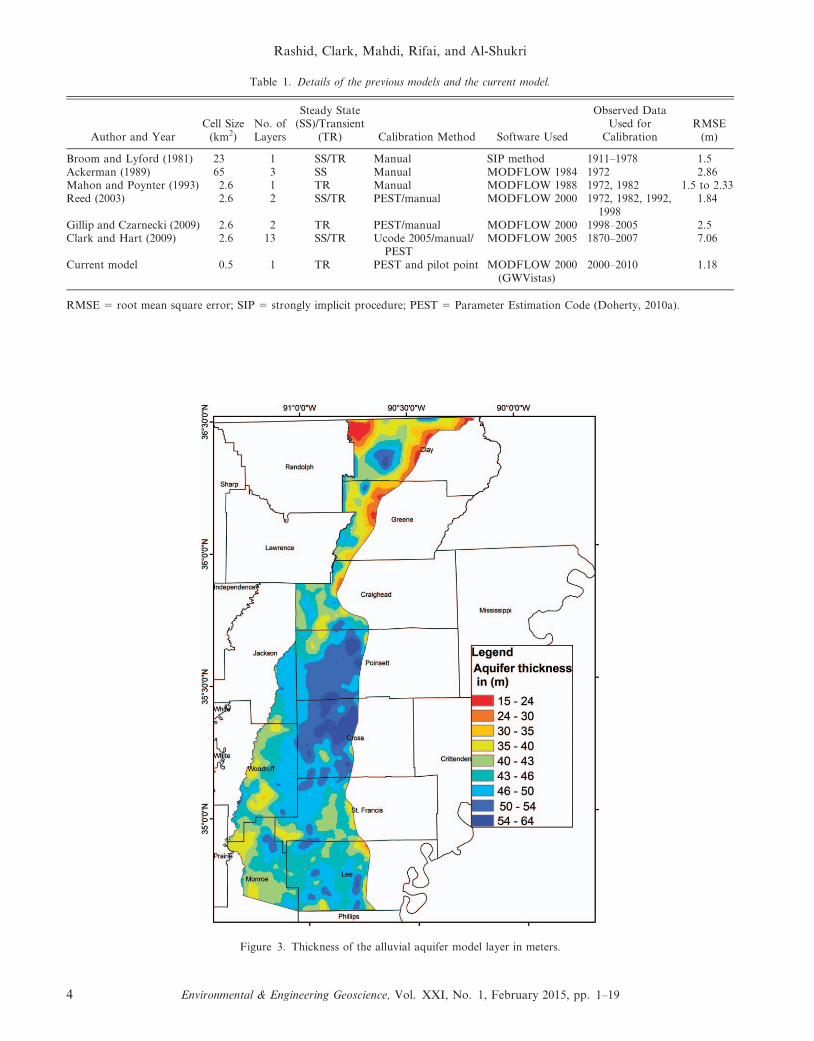
Table 1. Details of the previous models and the current model.

Author and YearCell Size

(km2)No. ofLayers

Steady State(SS)/Transient

(TR) Calibration Method Software Used

Observed DataUsed for

CalibrationRMSE

(m)

Broom and Lyford (1981) 23 1 SS/TR Manual SIP method 1911–1978 1.5Ackerman (1989) 65 3 SS Manual MODFLOW 1984 1972 2.86Mahon and Poynter (1993) 2.6 1 TR Manual MODFLOW 1988 1972, 1982 1.5 to 2.33Reed (2003) 2.6 2 SS/TR PEST/manual MODFLOW 2000 1972, 1982, 1992,

19981.84

Gillip and Czarnecki (2009) 2.6 2 TR PEST/manual MODFLOW 2000 1998–2005 2.5Clark and Hart (2009) 2.6 13 SS/TR Ucode 2005/manual/

PESTMODFLOW 2005 1870–2007 7.06

Current model 0.5 1 TR PEST and pilot point MODFLOW 2000(GWVistas)

2000–2010 1.18

RMSE 5 root mean square error; SIP 5 strongly implicit procedure; PEST 5 Parameter Estimation Code (Doherty, 2010a).

Figure 3. Thickness of the alluvial aquifer model layer in meters.



rice, soybeans, cotton, corn, sorghum, and wheat (U.S.Department of Agriculture, NRCS, 2011). Twoproposed irrigation project areas, L’Anguille Riverand Bayou DeView, of approximately 500 and427 km2, respectively, are located in part of each ofthe Craighead and Poinsett Counties (Czarnecki et al.,2003; U.S. Department of Agriculture, NRCS, 2011).Water use in the study area is dominantly for irrigation(Holland, 2007).

The alluvial aquifer is composed of alluvial andterrace deposits of Quaternary age (Ackerman, 1989).Lithologically, Quaternary alluvial and terrace depos-its are similar, consisting of unconsolidated sedimentsthat grade from gravel and coarse sand in the lowersections to silt and clay in the upper sections. The totalthickness of the alluvial aquifer ranges from 15 to 50 mand consists of coarse sand and gravel deposits. Theupper part of the alluvial aquifer (clay cap) consistsof clay, silt, and fine-grained sand that are generally

3–15 m thick (Czarnecki et al., 2002). The alluvialaquifer for most of the study area is unconfined, asdocumented in earlier studies (Czarnecki et al., 2002;Reed, 2003). Generally, within the study area, lateralflow of groundwater occurs from the north and westand flows toward the south and east. Crowley’s Ridge,which coincides with the easternmost part of the studyarea, is an erosional remnant of deposits of Tertiaryage trending north to south. Crowley’s Ridge is aprominent topographic feature compared to the low-relief surface of the Mississippi Alluvial Plain andforms a physical barrier to groundwater flow in thealluvial aquifer (Schrader, 2010).

Several groundwater flow models have been con-structed to simulate regional groundwater flow in thealluvial aquifer. Broom and Lyford (1981) developed atwo-dimensional digital model of the alluvial aquifer.Ackerman (1989) constructed a three-layer finite-difference model to simulate two-dimensional steady-

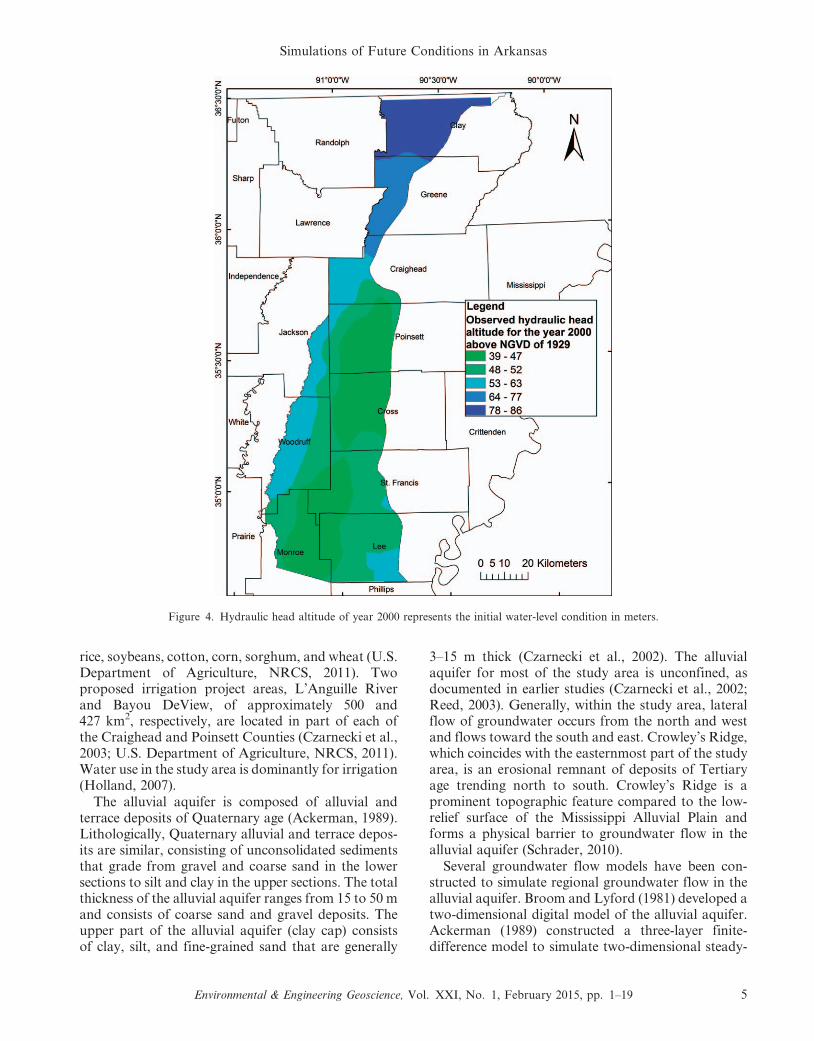
Figure 4. Hydraulic head altitude of year 2000 represents the initial water-level condition in meters.



state flow in the aquifer for the year 1972. Mahon andPoynter (1993) developed two separate models: one forthe area north of the Arkansas River and one for thearea south of the Arkansas River. Reed (2003)constructed a digital model of the alluvial aquifer ineastern Arkansas based on the model developed byMahon and Poynter (1993) to simulate groundwaterflow for the period from 1918 to 2049. Gillip andCzarnecki (2009) published a validation of the Reed(2003) groundwater flow model that was updated with1998–2005 water-use and water-level data. Clark andHart (2009) developed the Mississippi EmbaymentRegional Aquifer. Table 1 show details of the previousmodels and the current model.

METHODS

A numerical finite-difference model was construct-ed using Groundwater Vistas (version 6.18), which

provides a Windows graphical interface of MOD-FLOW. The MODFLOW 2000 (Harbaugh et al.,2000; Hill et al., 2000) and the PreconditionedConjugate-Gradient Method (PCG2) solver (Hill,1990) were used for simulation. The software wasused to solve the three-dimensional groundwater flowgoverning Eq. 1 (Anderson and Woessner, 1992).

LLx

KLh

Lx

� �z

LLy

KLh

Ly

� �z

LLz

KLh

Lz

� �{R~Ss

Lh

Ltð1Þ

where K is hydraulic conductivity; h is piezometric head;R is volumetric flux per unit volume (representingsource/sink terms); t is time; x, y, and z axes are assumedto be parallel to the major axes of the hydraulicconductivity; and Ss is specific storage coefficient.

The developed groundwater flow model simulates12,078 irrigation wells located in the study area thatwere pumped between 2000 and 2010. All wells were

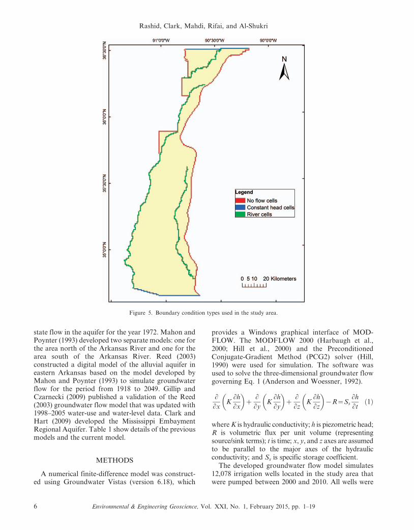
Figure 5. Boundary condition types used in the study area.



imported individually and represented using a wellpackage of MODFLOW; the summation of pumpingfor each model cell also was accomplished withinMODFLOW. Groundwater pumping from the allu-vial aquifer for irrigation is seasonal, occurringmainly from April to September (spring–summer),with little to no pumping from October to March(fall–winter). Most of the 10 counties located in thestudy area use groundwater at a rate of between 0.38and 1.5 million m3/d, except for Clay, Poinsett, andCross Counties, which have an estimated groundwa-ter use in the range of 1.5 to 4.5 million m3/d(Holland, 2007).

Model Discretization

The finite-difference grid used in the current modelconsists of 294 rows, 149 columns, and a single layerwith varying thickness by cell. Each model cellrepresents 0.5 km2 in area. The model simulation

represents 11 years (2000 to 2010) using 23 transientstress periods. Stress periods 2 to 23 are each 6 monthsin length to accommodate irrigation pumping occur-ring from April to September and the lack ofirrigation from October to March. All stress periodsare divided into six time steps (each time steprepresents a month in length) except for stress period1, which has three time steps.

River Package

The river package uses stream bed conductance(COND) to account for the length (L) and width (W)of the river channel in the cell, the thickness of theriver bed sediments (M), and their vertical hydraulicconductivity (Kv) (Anderson and Woessner, 1992),thus:

COND~KvLW

M,

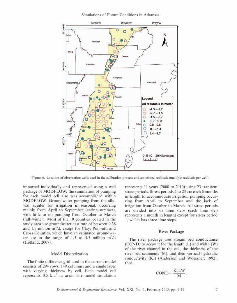
Figure 6. Location of observation wells used in the calibration process and associated residuals (multiple residuals per well).



where Kv was taken as 0.1 m/d for the Cache River and0.05 m/d for both the L’Anguille and Black Rivers as aninitial vertical hydraulic conductivity; W was taken asthe average width of the rivers measured from TOPOsoftware (version 3.4.3) as 19 m, 30 m, and 52 m forL’Anguille, Black, and Cache Rivers, respectively; andM was taken as 1 m. The total lengths (within the studyarea) of the simulated rivers were 62,049 m, 115,450 m,and 254,792 m for the Black, L’Anguille, and CacheRivers, respectively. The bottom of the rivers was takenas the same altitude of the datum of the gauges. Theriver stage data, taken from six gauges located on therivers (Figure 2), were downloaded for the years 2000to 2010 from the National Hydrography Dataset Plus.

The rate of leakage (Qriver) between the river andthe aquifer is calculated from the stream bedconductance, head in the river (Hriver), and head inthe aquifer (h) (Anderson and Woessner, 1992), thus:Qriver 5 COND (Hriver 2 h), for h . bottom of thestream bed (RBOT).

The leakage rate is calculated from Qriver 5

COND (Hriver 2 RBOT) for h # RBOT.

Layer Thickness

The layer thickness of the alluvial aquifer wasestimated using a Geographic Information System(Arc GIS10) by digitizing the two thickness contourmaps: 1) thickness of the Quaternary alluvial and

terrace deposits comprising the alluvial aquifer ineastern Arkansas (Pugh et al., 1997) and 2) thicknessof the Mississippi River Valley confining unit ineastern Arkansas (Gonthier and Mahon, 1993); thenthe thicknesses were added together to derive thelayer thickness. The top of the alluvial aquifer wasassumed to be land surface, and the bottom of thealluvial aquifer was calculated by subtracting thethickness of the aquifer from the top of the aquifer.Figure 3 shows the thickness of the model layer thatranged between 15 and 64 m. One layer was used tosimulate the alluvial aquifer. While this layer thick-ness includes the clay of the upper part of the aquifer,this inclusion is inconsequential in terms of aquiferproperties because the average depth of water isbelow the clay layer (Reed, 2003). Thus, whensimulated as a convertible layer, transmissivity,storage, and other head-dependent calculations arebased on the simulated water level rather than on thetop of the aquifer layer.

Model Parameters

The initial input model parameters, such ashydraulic conductivity and specific yield, assumed tobe homogeneous and isotropic, were 70 m/d (Pugh,2008) and 0.3 (dimensionless) (Broom and Lyford,1981; Anderson and Woessner, 1992; and Clark andHart, 2009), respectively. The recharge to the aquiferoccurs mainly from infiltration of precipitationthrough the upper fine-grained materials. Ground-water flow from the adjacent and underlying aquifersis assumed to be negligible and was neglected (Mahonand Poynter, 1993). The recharge rates of previousmodel simulations in the alluvial aquifer ranged from0.000055 to 0.00028 m/d (Ackerman, 1989; Mahonand Ludwig, 1989; and Clark and Hart, 2009). Theinitial recharge rate for this model was assumed to bea uniform rate of 0.00015 m/d.

Potentiometric Surfaces and InitialWater-Level Condition

Two aerially extensive cones of depression haveformed in the potentiometric surface in the CacheCritical Groundwater Area (Figure 4). One cone ofdepression occurs in Poinsett and Cross Counties(northern cone), and the second is in St. Francis, Lee,and Monroe Counties (southern cone). The potenti-ometric surface contours indicate that groundwaterflows toward the south and east, except where flow isaffected by groundwater withdrawals, such as in theareas of the cones of depression. More recently, thenorthern cone has expanded farther south into CrossCounty (Schrader, 2010). The potentiometric surface

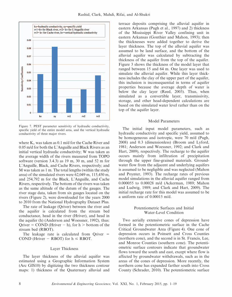
Figure 7. PEST parameter sensitivity of hydraulic conductivity,specific yield of the entire model area, and the vertical hydraulicconductivity of three major rivers.



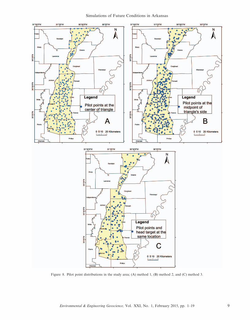
Figure 8. Pilot point distributions in the study area; (A) method 1, (B) method 2, and (C) method 3.



for the year 2000 was used as an initial water-levelcondition for the numerical model (Figure 4).

Boundary Conditions

In general, boundary conditions are mathematicalstatements specifying the dependent variable (head)or the derivative of the dependent variable (flux) at

the boundaries of the model domain. Boundaryconditions used in the model (Figure 5) consist ofthe constant head boundary condition for thenorthern and southern boundaries of the model.The specified head for the northern boundary changestemporally and ranges from 85 to 88 m. The southernspecified head boundary changes temporally andspatially and ranges between 45 and 57 m. For the

Table 2. Final parameter estimation from pilot point methods.

MethodTotal Number andType of Pilot Point Kx (m/d) Specific Yield Recharge (m/d) Residual Mean (m) RMS Error (m)

1 654_PH 42–173 0.1920.337 8.7 3 1025–6 3 1024 20.27 1.181 654_PV 41–175 0.18520.337 8.3 3 1025–6 3 1024 20.35 1.242 921_PH 43–172 0.18320.333 8.4 3 1025–6 3 1024 20.36 1.232 921_PV 43–180 0.18320.335 8.4 3 1025–6 3 1024 20.35 1.233 450_PH 43–169 0.18720.344 6.9 3 1025–6 3 1024 20.38 1.283 450_PV 43–169 0.18720.348 6.8 3 1025–6 3 1024 20.39 1.28

PH 5 preferred homogeneity; PV 5 preferred value.

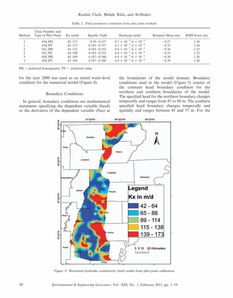
Figure 9. Horizontal hydraulic conductivity (m/d) results from pilot point calibration.



eastern boundary of the model, which coincides withCrowley’s Ridge, the no-flow boundary condition wasapplied because the ridge functions as a groundwaterflow barrier. For most of the western boundary ofthe area, the river boundary condition was applied (theCache River being the actual boundary) using theMODFLOW river package.

Calibration

Calibration is the process of adjusting model inputparameter values to match the simulated values to thefield observations. Simulated heads were compared to2,322 hydraulic head observations from 150 observa-tion wells completed in Quaternary alluvium andterrace deposits located in the study area (Figure 6).The model was calibrated in two phases. The firstphase used the parameter estimation code (PEST)process (Doherty, 2010a, 2010b), which assumes thestudy area is homogeneous and isotropic and was

used to determine the sensitivity of model results tooverall aquifer properties. In the second phase, a pilotpoint technique was used in three different ways,described in the following section, to evaluate pilotpoint distribution effects on model calibration. Theparameters estimated in the first phase included thehorizontal hydraulic conductivity, the specific yield,and the river conductance for all three simulatedrivers. The most sensitive parameters were specificyield (sy), hydraulic conductivity (kx), and riververtical hydraulic conductivity for the Cache River(rv3), L’Anguille River (rv2), and Black River (rv1),respectively (Figure 7). Thus, pilot point calibrationwas undertaken to improve the spatial distribution,and consequently the calibration, of these variables.

Pilot Points

In the second phase of model calibration, pilotpoints were used with regularization and Singular

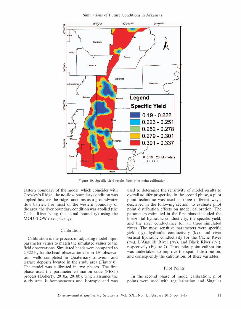
Figure 10. Specific yield results from pilot point calibration.



Value Decomposition assist to improve the spatialvariation in parameter values and the model calibra-tion. The aim of using pilot points is to provide anintermediate approach for characterizing heterogene-ity in groundwater models between direct representa-tion of cell by cell variability and reduction ofparameterization to a relatively few homogeneouszones (Doherty et al., 2010).

Pilot points allow for greater flexibility in thespatial assignment of the aquifer properties. Eachpoint at a specified location can be assigned a value ofa hydraulic property, which can change throughoutthe calibration process. A hydraulic property valuefor each model cell is interpolated based on the valuesof surrounding pilot points, which can serve tospatially vary the properties in a gradational manner,rather than as fixed discrete zones of hydraulicproperties. For more information on pilot pointsand geostatistical methods associated with their usesee Doherty (2013).

Pilot point parameter values were estimated at anumber of discrete locations distributed throughoutthe model domain, and these parameter values werethen spatially interpolated to the cells of the model gridusing a kriging spatial interpolation method (Doherty,2010a). Three different distributions of the pilot pointswere used (Rashid et al., 2013) (Figure 8), as follows:1) observation triangulation method using preferredhomogeneity regularization in which a triangle foreach neighboring observation well was constructedand pilot points were specified at the center of eachtriangle (Rumbaugh and Rumbaugh, 2011); 2) similarto method 1; however, the pilot points were specified atthe midpoints of each side of a given triangle; and 3)pilot points specified exactly at the same location ofobservation wells. For all three methods, additionalpilot points were included to fill in gaps (areas that didnot have pilot points within a 7-km radius). The totalnumbers of pilot points were 654, 921, and 450 formethods 1, 2, and 3, respectively (Figure 8). For each

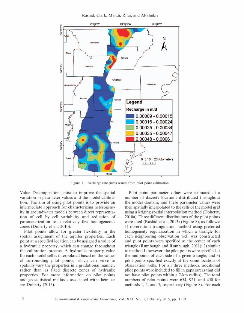
Figure 11. Recharge rate (m/d) results from pilot point calibration.



of the parameter groups—hydraulic conductivity,specific yield, and recharge—218, 307, and 150 pilotpoints were used in methods 1, 2, and 3, respectively.The pilot point distribution method 1 using theobservation triangulation method (654 pilot points)with preferred homogeneity regularization was chosenas the final model calibration because of the lower rootmean square error (RMSE) in comparison with thoseof the other pilot point distributions, althoughdifferences in RMSE among the three methods wererelatively small, on the order of 0.1 m (Table 2).

RESULTS

The final parameter estimates for the calibratedmodel (Figures 9 through 11) were considered reason-able estimates based on the simulations that werecompleted as well as on previous studies for the materialtype and condition found in the alluvial aquifer.Horizontal hydraulic conductivity ranged from 42 to

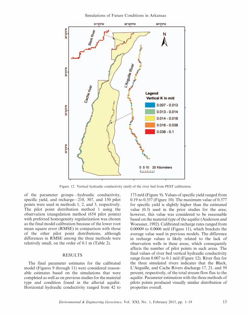
173 m/d (Figure 9). Values of specific yield ranged from0.19 to 0.337 (Figure 10). The maximum value of 0.377for specific yield is slightly higher than the estimatedvalue (0.3) used in the prior studies for the area;however, this value was considered to be reasonablebased on the material type of the aquifer (Anderson andWoessner, 1992). Calibrated recharge rates ranged from0.00009 to 0.0006 m/d (Figure 11), which brackets theaverage value used in previous models. The differencein recharge values is likely related to the lack ofobservation wells in these areas, which consequentlyaffects the number of pilot points in such areas. Thefinal values of river bed vertical hydraulic conductivityrange from 0.007 to 0.1 m/d (Figure 12). River flux forthe three simulated rivers indicates that the Black,L’Anguille, and Cache Rivers discharge 17, 21, and 59percent, respectively, of the total stream flow flux to theaquifer. Parameter estimation with the three methods ofpilots points produced visually similar distribution ofproperties overall.

Figure 12. Vertical hydraulic conductivity (m/d) of the river bed from PEST calibration.



Hydraulic Head Observations and Error

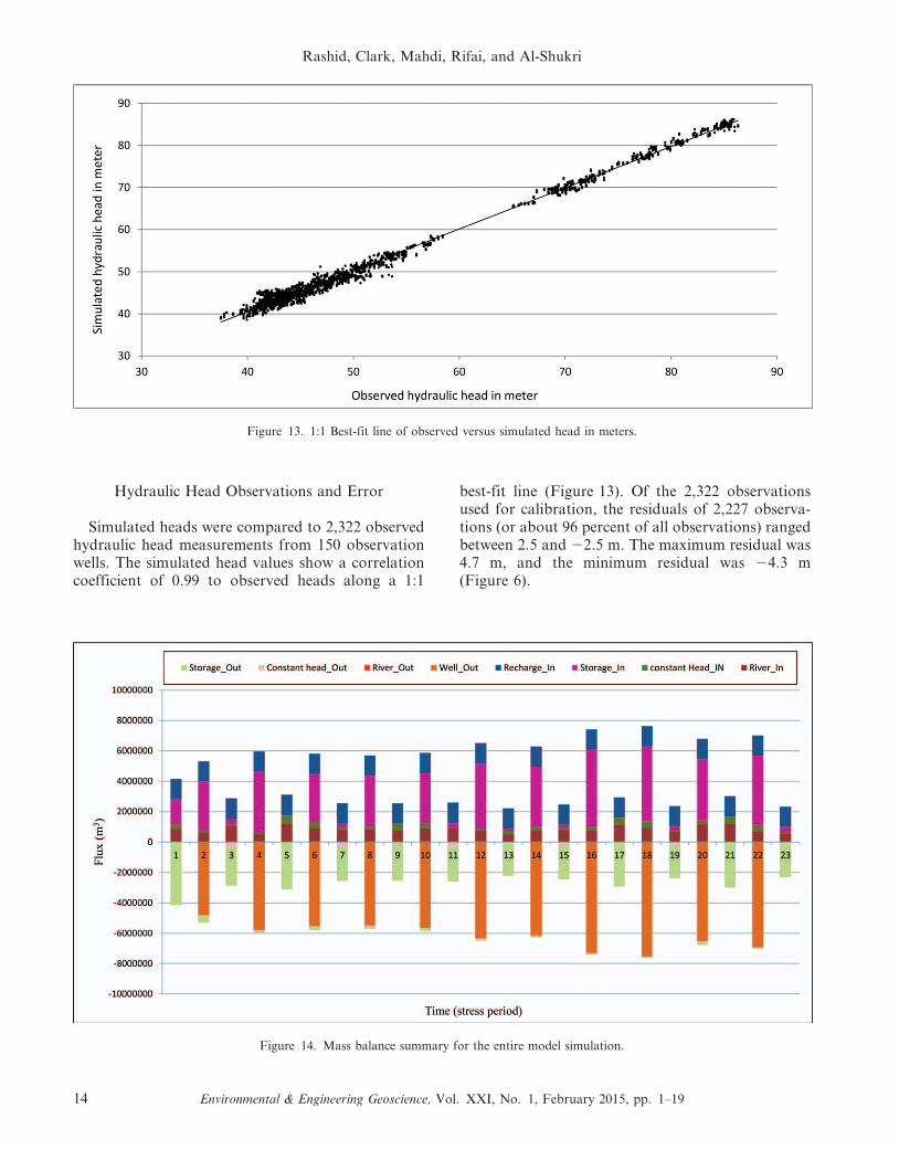
Simulated heads were compared to 2,322 observedhydraulic head measurements from 150 observationwells. The simulated head values show a correlationcoefficient of 0.99 to observed heads along a 1:1

best-fit line (Figure 13). Of the 2,322 observationsused for calibration, the residuals of 2,227 observa-tions (or about 96 percent of all observations) rangedbetween 2.5 and 22.5 m. The maximum residual was4.7 m, and the minimum residual was 24.3 m(Figure 6).

Figure 13. 1:1 Best-fit line of observed versus simulated head in meters.

Figure 14. Mass balance summary for the entire model simulation.



RMSE was determined using the equation

RMSE~½Sum(ho{hs)2=n�0:5

(ho{hs) is residual in meters

where ho is observed hydraulic head in meters; hs issimulated hydraulic head in meters, and n is numberof observations.

The average value of the RMSE for the first phase ofcalibration was 1.64 m, whereas the values of theRMSE for the second phase ranged from 0.94 m in2002 to 1.45 m in 2008, with an average of 1.18 m over arange of observed hydraulic head of 48.84 m (the rangeequals the difference between the highest and lowestobserved hydraulic head). The mean of residualsindicates model bias depending on the magnitude anddirection of the mean away from zero (Clark and Hart,2009). The closer the mean to zero, the less model biasoccurs. A positive mean indicates that the model tendsto under-predict, and a negative mean indicates themodel tends to over-predict. The mean residual for theentire model simulation was 20.27 m, which indicates aslight bias of simulated heads to over-predict theobserved hydraulic heads. Out of 2,322 observations,

1,374 residuals (59.18 percent) were less than zero(over-prediction), and 948 residuals (40.82 percent)were greater than zero (under-prediction).

Mass Balance

The mass balance summary, which indicateschanges in storage, for all inflow to the aquifer andoutflow from the aquifer for the entire modelsimulation (23 stress periods) is shown in Figure 14.Positive rates indicate inflows to the aquifer, andnegative rates indicate outflows from the aquifer. Thepercent error between the inflow to the aquifer andoutflow from the aquifer was equal to 23.79 3 1025.

Withdrawal Scenarios

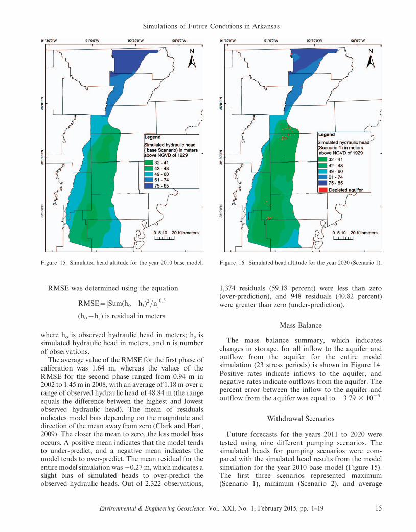
Future forecasts for the years 2011 to 2020 weretested using nine different pumping scenarios. Thesimulated heads for pumping scenarios were com-pared with the simulated head results from the modelsimulation for the year 2010 base model (Figure 15).The first three scenarios represented maximum(Scenario 1), minimum (Scenario 2), and average

Figure 15. Simulated head altitude for the year 2010 base model. Figure 16. Simulated head altitude for the year 2020 (Scenario 1).



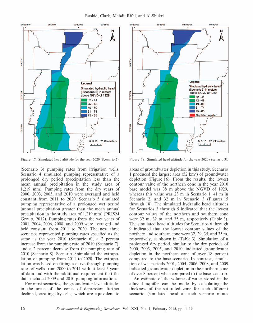
(Scenario 3) pumping rates from irrigation wells.Scenario 4 simulated pumping representative of aprolonged dry period (precipitation less than themean annual precipitation in the study area of1,219 mm). Pumping rates from the dry years of2000, 2003, 2005, and 2010 were averaged and heldconstant from 2011 to 2020. Scenario 5 simulatedpumping representative of a prolonged wet period(annual precipitation greater than the mean annualprecipitation in the study area of 1,219 mm) (PRISMGroup, 2012). Pumping rates from the wet years of2001, 2004, 2006, 2008, and 2009 were averaged andheld constant from 2011 to 2020. The next threescenarios represented pumping rates specified as thesame as the year 2010 (Scenario 6), a 2 percentincrease from the pumping rate of 2010 (Scenario 7),and a 2 percent decrease from the pumping rate of2010 (Scenario 8). Scenario 9 simulated the extrapo-lation of pumping from 2011 to 2020. The extrapo-lation was based on fitting a curve through pumpingrates of wells from 2000 to 2011 with at least 5 yearsof data and with the additional requirement that thedata included 2009 and 2010 pumping information.

For most scenarios, the groundwater level altitudesin the areas of the cones of depression furtherdeclined, creating dry cells, which are equivalent to

areas of groundwater depletion in this study. Scenario1 produced the largest area (52 km2) of groundwaterdepletion (Figure 16). From the results, the lowestcontour value of the northern cone in the year 2010base model was 38 m above the NGVD of 1929,whereas this value was 23 m in Scenario 1, 41 m inScenario 2, and 32 m in Scenario 3 (Figures 15through 18). The simulated hydraulic head altitudesfor Scenarios 3 through 5 indicated that the lowestcontour values of the northern and southern conewere 32 m, 32 m, and 35 m, respectively (Table 3).The simulated head altitudes for Scenarios 6 through9 indicated that the lowest contour values of thenorthern and southern cone were 32, 29, 35, and 35 m,respectively, as shown in (Table 3). Simulation of aprolonged dry period, similar to the dry periods of2000, 2003, 2005, and 2010, indicated groundwaterdepletion in the northern cone of over 18 percentcompared to the base scenario. In contrast, simula-tion of wet periods 2001, 2004, 2006, 2008, and 2009indicated groundwater depletion in the northern coneof over 8 percent when compared to the base scenario.

An estimate of the volume of water stored in thealluvial aquifer can be made by calculating thethickness of the saturated zone for each differentscenario (simulated head at each scenario minus

Figure 17. Simulated head altitude for the year 2020 (Scenario 2). Figure 18. Simulated head altitude for the year 2020 (Scenario 3).



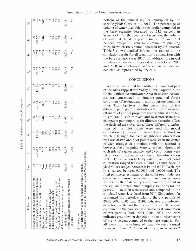
bottom of the alluvial aquifer, multiplied by thespecific yield; Clark et al., 2011). The percentage ofvolume of water available in the aquifer compared tothe base scenario decreased by 23.3 percent inScenario 1. For the nine tested scenarios, the volumeof water depleted ranged between 5.7 and 23.3percent, except in Scenario 2 (minimum pumpingrate), in which the volume increased by 2.5 percent.Table 3 shows detailed information related to thesimulation results for all scenarios in comparison withthe base scenario (year 2010). In addition, the modelsimulations indicated the period of time between 2011and 2020, in which areas of the alluvial aquifer aredepleted, as represented by dry cells.

CONCLUSIONS

A three-dimensional finite-difference model of partof the Mississippi River Valley alluvial aquifer in theCache Critical Groundwater Area in eastern Arkan-sas was constructed to simulate potential futureconditions of groundwater heads at various pumpingrates. The objectives of this study were to testdifferent pilot point distributions to find reasonableestimates of aquifer properties for the alluvial aquifer,to simulate flux from rivers and to demonstrate howchanges in pumping rates for different scenarios affectthe depleted area over time. Three different distribu-tions of the pilot points were used for modelcalibration: 1) observation triangulation method, inwhich a triangle for each neighboring observationwell was drawn and pilot points were set in the centerof each triangle; 2) a method similar to method 1;however, the pilot points were set at the midpoints ofeach side of a given triangle; and 3) pilot points wereset at exactly the same location of the observationwells. Hydraulic conductivity values from pilot pointcalibration ranged between 42 and 173 m/d. Specificyield values ranged between 0.19 and 0.337. Rechargerates ranged between 0.00009 and 0.0006 m/d. Thefinal parameter estimates of the calibrated model areconsidered reasonable estimates based on previousstudies for the material type and condition found inthe alluvial aquifer. Nine pumping scenarios for theyears 2011 to 2020 were tested and compared to thesimulated water-level head from 2010. Simulation of aprolonged dry period, similar to the dry periods of2000, 2003, 2005, and 2010, indicates groundwaterdepletion in the northern cone of over 18 percentcompared to the base scenario; in contrast, simulationof wet periods 2001, 2004, 2006, 2008, and 2009indicates groundwater depletion in the northern coneof over 8 percent compared to the base scenario. Forall scenarios the volume of water depleted rangedbetween 5.7 and 23.3 percent, except in Scenario 2

Ta

ble

3.

Sim

ula

tio

nre

sult

so

fa

llsc

ena

rio

s.

Info

rma

tio

nB

ase

S1

S2

S3

S4

S5

S6

S7

S8

S9

Lo

wes

tco

nto

ur

va

lue

for

no

rth

ern

con

e1(m

)3

82

34

13

23

23

53

22

93

53

5R

an

ge

inth

ed

iffe

ren

cein

sim

ula

ted

hea

d(m

)0

20

.22

–2

0.7

24

.3–

2.6

21

.4–

7.9

22

.2–

8.1

21

.8–

7.7

22

.5–

7.9

21

.6–

9.0

22

.8–

5.9

21

.1–

7.2

Lo

wes

tco

nto

ur

va

lue

for

sou

ther

nco

ne2

(m)

38

20

41

32

32

32

32

29

35

35

Dry

cell

sta

rty

ear

N/A

20

12

N/A

20

16

20

13

20

12

20

14

20

13

20

16

20

13

No

.o

fd

ryce

lls

as

sta

rted

N/A

6N

/A2

31

12

11

To

tal

no

.o

fd

ryce

lls

at

yea

r2

02

0N

/A1

04

N/A

89

58

10

58

To

tal

pu

mp

ing

rate

(mil

lio

nm

3)

6.9

12

.43

.57

.57

.27

.46

.98

.35

.57

.3P

erce

nt

incr

ease

/dec

rea

seo

fp

um

pin

gra

te0

.07

8.6

25

0.0

8.1

4.2

6.4

0.0

19

.32

20

.25

.8M

ean

hea

do

fw

ate

rst

ore

din

the

aq

uif

er(m

)8

.26

.38

.57

.67

.67

.67

.67

.57

.87

.8V

olu

me

of

wa

ter

sto

red

inth

ea

qu

ifer

(mil

lio

nm

3)

56

,63

64

3,4

25

58

,06

45

1,9

57

52

,08

65

2,2

08

52

,44

45

1,2

74

53

,42

05

3,3

14

Per

cen

td

ecre

ase

/in

crea

seo

fst

ore

dv

olu

me

of

wa

ter

0.0

22

3.3

2.5

28

.32

8.0

27

.82

7.4

29

.52

5.7

25

.9

S5

scen

ari

o.

1N

ort

her

nco

ne

5co

ne

inP

oin

sett

an

dC

ross

Co

un

ties

.2S

ou

ther

nco

ne

5co

ne

inS

t.F

ran

cis,

Lee

,a

nd

Mo

nro

eC

ou

nti

es.



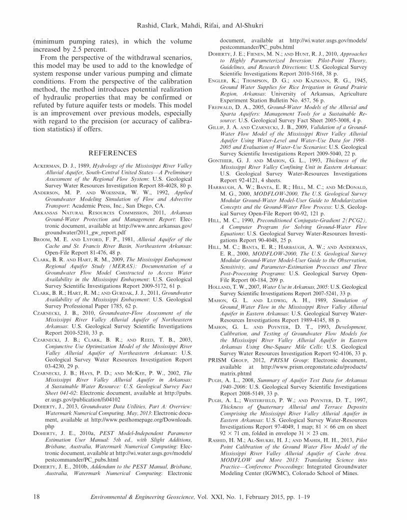
(minimum pumping rates), in which the volumeincreased by 2.5 percent.

From the perspective of the withdrawal scenarios,this model may be used to add to the knowledge ofsystem response under various pumping and climateconditions. From the perspective of the calibrationmethod, the method introduces potential realizationof hydraulic properties that may be confirmed orrefuted by future aquifer tests or models. This modelis an improvement over previous models, especiallywith regard to the precision (or accuracy of calibra-tion statistics) if offers.

REFERENCES

ACKERMAN, D. J., 1989, Hydrology of the Mississippi River ValleyAlluvial Aquifer, South-Central United States—A PreliminaryAssessment of the Regional Flow System: U.S. GeologicalSurvey Water Resources Investigation Report 88-4028, 80 p.

ANDERSON, M. P. AND WOESSNER, W. W., 1992, AppliedGroundwater Modeling Simulation of Flow and AdvectiveTransport: Academic Press, Inc., San Diego, CA.

ARKANSAS NATURAL RESOURCES COMMISSION, 2011, ArkansasGround-Water Protection and Management Report: Elec-tronic document, available at http://www.anrc.arkansas.gov/groundwater/2011_gw_report.pdf

BROOM, M. E. AND LYFORD, F. P., 1981, Alluvial Aquifer of theCache and St. Francis River Basin, Northeastern Arkansas:Open-File Report 81-476, 48 p.

CLARK, B. R. AND HART, R. M., 2009, The Mississippi EmbaymentRegional Aquifer Study (MERAS): Documentation of aGroundwater Flow Model Constructed to Access WaterAvailability in the Mississippi Embayment: U.S. GeologicalSurvey Scientific Investigations Report 2009-5172, 61 p.

CLARK, B. R.; HART, R. M.; AND GURDAK, J. J., 2011, GroundwaterAvailability of the Mississippi Embayment: U.S. GeologicalSurvey Professional Paper 1785, 62 p.

CZARNECKI, J. B., 2010, Groundwater-Flow Assessment of theMississippi River Valley Alluvial Aquifer of NortheasternArkansas: U.S. Geological Survey Scientific InvestigationsReport 2010-5210, 33 p.

CZARNECKI, J. B.; CLARK, B. R.; AND REED, T. B., 2003,Conjunctive Use Optimization Model of the Mississippi RiverValley Alluvial Aquifer of Northeastern Arkansas: U.S.Geological Survey Water Resources Investigation Report03-4230, 29 p.

CZARNECKI, J. B.; HAYS, P. D.; AND MCKEE, P. W., 2002, TheMississippi River Valley Alluvial Aquifer in Arkansas:A Sustainable Water Resource: U.S. Geological Survey FactSheet 041-02: Electronic document, available at http://pubs.er.usgs.gov/publication/fs04102

DOHERTY, J., 2013, Groundwater Data Utilities, Part A: Overview:Watermark Numerical Computing, May, 2013: Electronic docu-ment, available at http://www.pesthomepage.org/Downloads.php

DOHERTY, J. E., 2010a, PEST Model-Independent ParameterEstimation User Manual: 5th ed., with Slight Additions,Brisbane, Australia, Watermark Numerical Computing: Elec-tronic document, available at http://wi.water.usgs.gov/models/pestcommander/PC_pubs.html

DOHERTY, J. E., 2010b, Addendum to the PEST Manual, Brisbane,Australia, Watermark Numerical Computing: Electronic

document, available at http://wi.water.usgs.gov/models/pestcommander/PC_pubs.html

DOHERTY, J. E.; FIENEN, M. N.; AND HUNT, R. J., 2010, Approachesto Highly Parameterized Inversion: Pilot-Point Theory,Guidelines, and Research Directions: U.S. Geological SurveyScientific Investigations Report 2010-5168, 38 p.

ENGLER, K.; THOMPSON, D. G.; AND KAZMANN, R. G., 1945,Ground Water Supplies for Rice Irrigation in Grand PrairieRegion, Arkansas: University of Arkansas, AgricultureExperiment Station Bulletin No. 457, 56 p.

FREIWALD, D. A., 2005, Ground-Water Models of the Alluvial andSparta Aquifers: Management Tools for a Sustainable Re-source: U.S. Geological Survey Fact Sheet 2005-3008, 4 p.

GILLIP, J. A. AND CZARNECKI, J. B., 2009, Validation of a Ground-Water Flow Model of the Mississippi River Valley AlluvialAquifer Using Water-Level and Water-Use Data for 1998–2005 and Evaluation of Water-Use Scenarios: U.S. GeologicalSurvey Scientific Investigations Report 2009-5040, 22 p.

GONTHIER, G. J. AND MAHON, G. L., 1993, Thickness of theMississippi River Valley Confining Unit in Eastern Arkansas:U.S. Geological Survey Water-Resources InvestigationsReport 92-4121, 4 sheets.

HARBAUGH, A. W.; BANTA, E. R.; HILL, M. C.; AND MCDONALD,M. G., 2000, MODFLOW-2000, The U.S. Geological SurveyModular Ground-Water Model-User Guide to ModularizationConcepts and the Ground-Water Flow Process: U.S. Geolog-ical Survey Open-File Report 00-92, 121 p.

HILL, M. C., 1990, Preconditioned Conjugate-Gradient 2(PCG2),A Computer Program for Solving Ground-Water FlowEquations: U.S. Geological Survey Water-Resources Investi-gations Report 90-4048, 25 p.

HILL, M. C.; BANTA, E. R.; HARBAUGH, A. W.; AND ANDERMAN,E. R., 2000, MODFLOW-2000, The U.S. Geological SurveyModular Ground-Water Model-User Guide to the Observation,Sensitivity, and Parameter-Estimation Processes and ThreePost-Processing Programs: U.S. Geological Survey Open-File Report 00-184, 209 p.

HOLLAND, T. W., 2007, Water Use in Arkansas, 2005: U.S. GeologicalSurvey Scientific Investigations Report 2007-5241, 33 p.

MAHON, G. L. AND LUDWIG, A. H., 1989, Simulation ofGround_Water Flow in the Mississippi River Valley AlluvialAquifer in Eastern Arkansas: U.S. Geological Survey Water-Resources Investigations Report 1989-4145, 88 p.

MAHON, G. L. AND POYNTER, D. T., 1993, Development,Calibration, and Testing of Groundwater Flow Models forthe Mississippi River Valley Alluvial Aquifer in EasternArkansas Using One-Square Mile Cells: U.S. GeologicalSurvey Water Resources Investigation Report 92-4106, 33 p.

PRISM GROUP, 2012, PRISM Group: Electronic document,available at http://www.prism.oregonstate.edu/products/matrix.phtml

PUGH, A. L., 2008, Summary of Aquifer Test Data for Arkansas1940–2006: U.S. Geological Survey Scientific InvestigationsReport 2008-5149, 33 p.

PUGH, A. L.; WESTERFIELD, P. W.; AND POYNTER, D. T., 1997,Thickness of Quaternary Alluvial and Terrace DepositsComprising the Mississippi River Valley Alluvial Aquifer inEastern Arkansas: U.S. Geological Survey Water-ResourcesInvestigations Report 97-4049, 1 map; 81 3 66 cm on sheet92 3 71 cm, folded in envelope 31 3 23 cm.

RASHID, H. M.; AL-SHUKRI, H. J.; AND MAHDI, H. H., 2013, PilotPoint Calibration of the Ground Water Flow Model of theMississippi River Valley Alluvial Aquifer of Cache Area.MODFLOW and More 2013: Translating Science intoPractice—Conference Proceedings: Integrated GroundwaterModeling Center (IGWMC), Colorado School of Mines.



REED, T. B., 2003, Recalibration of a Ground-Water Model of theMississippi River Valley Alluvial Aquifer of Northeast Arkansas,1918–1998, with Simulations of Water Levels Caused by ProjectedGround-Water Withdrawals through 2049: U.S. GeologicalSurvey Water Resources Investigations Report 2003-4109, 58 p.

RUMBAUGH, J. O. AND RUMBAUGH, D. B., 2011, Guide to UsingGroundwater Vistas, version 6: Environmental Simulations, Inc.,Reinholds, PA.

SCHRADER, T. P., 2010, Water Levels and Selected Water-QualityConditions in the Mississippi River Valley Alluvial Aquiferin Eastern Arkansas, 2008: U.S. Geological Survey Water-Resources Scientific Investigations Report 2010-5140,71 p.

U.S. DEPARTMENT OF AGRICULTURE, NRCS, 2011, IrrigationProjects: Electronic document, available at http://www.ar.nrcs.usda.gov/programs/watersheds_irrigation.html



Uncertainty Associated with Evaluating Rockfall

Hazard to Roads in Burned Areas

JEROME V. DE GRAFF1

USDA Forest Service, 1600 Tollhouse Road, Clovis, CA 93611

BILL SHELMERDINE

Olympic National Forest, 1835 Black Lake Boulevard, SW, Olympia, WA 98512

ALAN GALLEGOS

USDA Forest Service, 1600 Tollhouse Road, Clovis, CA 93611

DAVID ANNIS

Eldorado National Forest, 100 Forni Road, Placerville, CA 95667

Key Terms: Rockfall, Wildfires, Roads, Western USA,Natural Hazards

ABSTRACT

During and following wildfires affecting steep mountainslopes, there can be an increase in rockfall activity usuallytaking the form of individual rocks, and occasionally,groups of rocks rolling, sliding or bouncing downslope.This increase results from removal of stabilizing vegeta-tion, downed wood, and organics within the soil matrix aswell as increase in erosional processes such as dry ravel.The hazard posed to vehicles is difficult to assess becauseof uncertainty manifested in several ways. First, there isuncertainty in defining the road segments that will beimpacted by increased rockfall activity. Second, it isdifficult to quantify the size, number, and/or travelbehavior of rocks which may impact a given roadsegment. Finally, there is uncertainty as to how longincreased rockfall activity may persist after a wildfire.Between 2007 and 2013, some insight into the first twouncertainty issues was provided by observed rockfall onroads within eight different wildfires in California andIdaho. This insight provided an efficient and effectivemeans to prioritize rapid assessment for rockfall hazardfor a large number of roads within the 2013 Rim Fire inthe central Sierra Nevada, California. Data on the thirdrockfall uncertainty issue, persistence, was developed fora road on the Olympic National Forest in Washington.Monitoring of rocks accumulating on the road at sixteensites between July 2006 and April 2007 recorded 3,463

rocks with the number of rocks found to decrease overtime.

INTRODUCTION

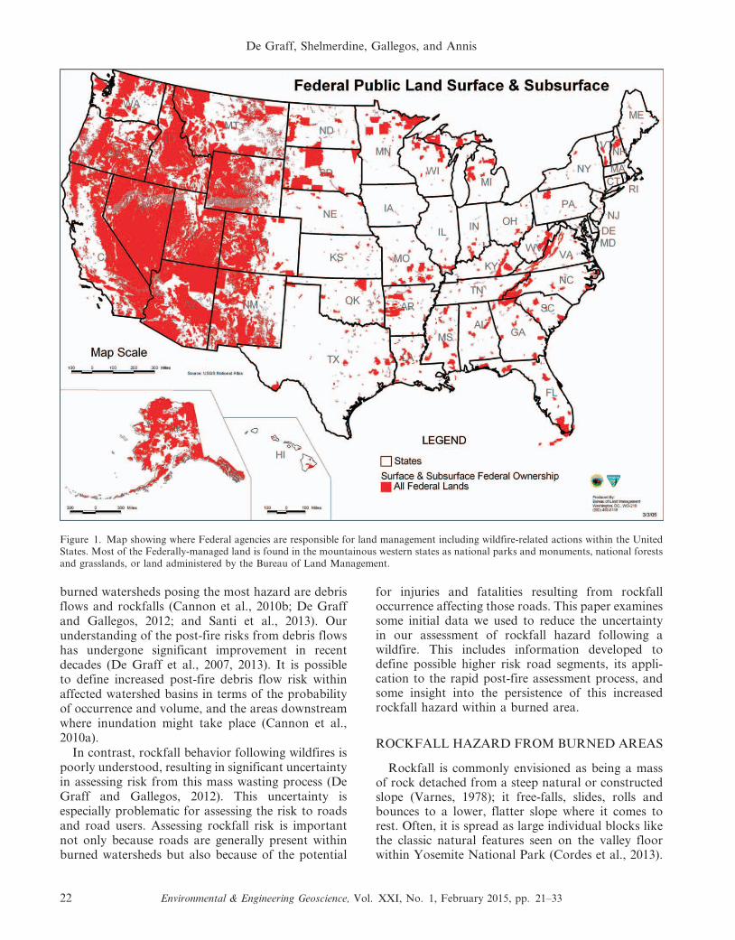
Since the 1980s, wildfires occurring in the westernUnited States have increased on the basis of eitherarea being burned (Stephens, 2005) or frequency(Westerling et al., 2006). Much of this increasingtrend can be attributed to climatic control (Littell etal., 2009). Commonly, western wildfires are concen-trated in mountainous landscapes often involvingland administered by Federal agencies including theForest Service, National Park Service and Bureau ofLand Management (Figure 1).

The mountainous areas of the western United Statesare largely rural in character with fewer roads than arefound within the major valleys and plains boundingthem. The steep slopes limit most of the Interstate andState highways to certain corridors across the mountainranges. Local roads are typically more numerous andexist to access mountain communities, residences,energy development sites, ski resorts and other recrea-tional facilities, mining operations, and to carry outland management activities such as timber harvest andfire suppression. Many roads in these mountainousareas are subject to landslide impacts which interferewith their intended uses, threaten public safety, andimpose significant hardship on road users (De Graffand Cunningham, 1982; De Graff et al., 1984; Cannonet al., 2001; Harp et al., 2008; and Beukelman andErickson, 2012).

Landslide activity can be greater after a wildfire,increasing the risk posed to roads within the burnedarea. The landslide types commonly associated with1Corresponding author email: [email protected].


burned watersheds posing the most hazard are debrisflows and rockfalls (Cannon et al., 2010b; De Graffand Gallegos, 2012; and Santi et al., 2013). Ourunderstanding of the post-fire risks from debris flowshas undergone significant improvement in recentdecades (De Graff et al., 2007, 2013). It is possibleto define increased post-fire debris flow risk withinaffected watershed basins in terms of the probabilityof occurrence and volume, and the areas downstreamwhere inundation might take place (Cannon et al.,2010a).

In contrast, rockfall behavior following wildfires ispoorly understood, resulting in significant uncertaintyin assessing risk from this mass wasting process (DeGraff and Gallegos, 2012). This uncertainty isespecially problematic for assessing the risk to roadsand road users. Assessing rockfall risk is importantnot only because roads are generally present withinburned watersheds but also because of the potential

for injuries and fatalities resulting from rockfalloccurrence affecting those roads. This paper examinessome initial data we used to reduce the uncertaintyin our assessment of rockfall hazard following awildfire. This includes information developed todefine possible higher risk road segments, its appli-cation to the rapid post-fire assessment process, andsome insight into the persistence of this increasedrockfall hazard within a burned area.

ROCKFALL HAZARD FROM BURNED AREAS

Rockfall is commonly envisioned as being a massof rock detached from a steep natural or constructedslope (Varnes, 1978); it free-falls, slides, rolls andbounces to a lower, flatter slope where it comes torest. Often, it is spread as large individual blocks likethe classic natural features seen on the valley floorwithin Yosemite National Park (Cordes et al., 2013).

Figure 1. Map showing where Federal agencies are responsible for land management including wildfire-related actions within the UnitedStates. Most of the Federally-managed land is found in the mountainous western states as national parks and monuments, national forestsand grasslands, or land administered by the Bureau of Land Management.

De Graff, Shelmerdine, Gallegos, and Annis


Rockfall from large individual boulders or multiplelarge rocks can also be generated from slopes mantledby glacial, fluvial, or colluvial deposits. This is oftenin response to the erosional loss of the fine-grainedmatrix surrounding these large rock blocks (Turnerand Jayprakash, 2012). Turner and Jayprakash (2012)point out that while large rockfalls can blocktransportation corridors for days, rockfalls involvingrelatively small volumes can pose significant hazardsto travelers, recreationists, and workers.

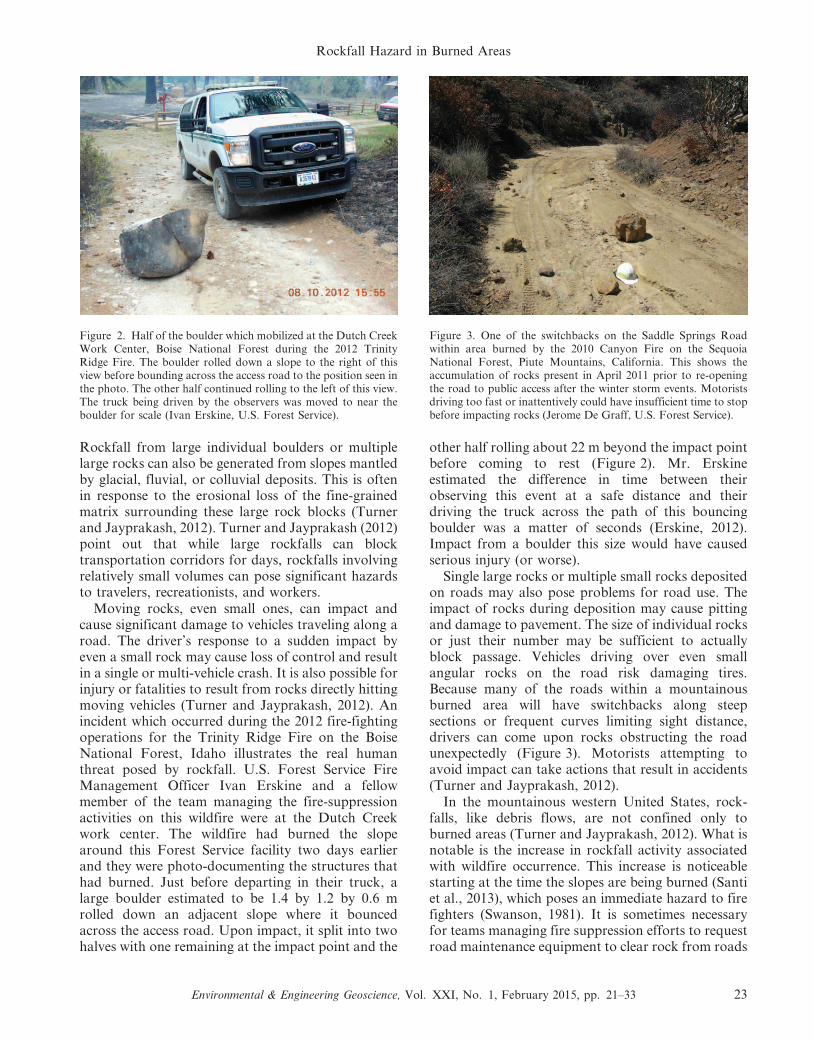
Moving rocks, even small ones, can impact andcause significant damage to vehicles traveling along aroad. The driver’s response to a sudden impact byeven a small rock may cause loss of control and resultin a single or multi-vehicle crash. It is also possible forinjury or fatalities to result from rocks directly hittingmoving vehicles (Turner and Jayprakash, 2012). Anincident which occurred during the 2012 fire-fightingoperations for the Trinity Ridge Fire on the BoiseNational Forest, Idaho illustrates the real humanthreat posed by rockfall. U.S. Forest Service FireManagement Officer Ivan Erskine and a fellowmember of the team managing the fire-suppressionactivities on this wildfire were at the Dutch Creekwork center. The wildfire had burned the slopearound this Forest Service facility two days earlierand they were photo-documenting the structures thathad burned. Just before departing in their truck, alarge boulder estimated to be 1.4 by 1.2 by 0.6 mrolled down an adjacent slope where it bouncedacross the access road. Upon impact, it split into twohalves with one remaining at the impact point and the

other half rolling about 22 m beyond the impact pointbefore coming to rest (Figure 2). Mr. Erskineestimated the difference in time between theirobserving this event at a safe distance and theirdriving the truck across the path of this bouncingboulder was a matter of seconds (Erskine, 2012).Impact from a boulder this size would have causedserious injury (or worse).

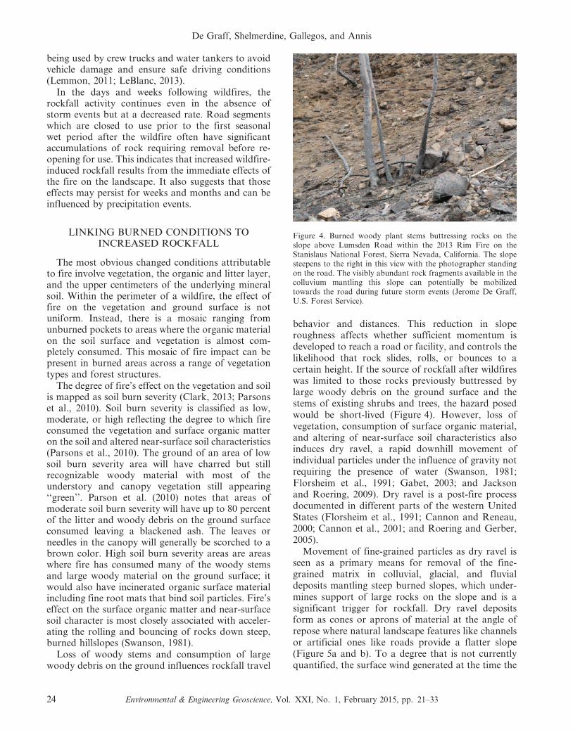
Single large rocks or multiple small rocks depositedon roads may also pose problems for road use. Theimpact of rocks during deposition may cause pittingand damage to pavement. The size of individual rocksor just their number may be sufficient to actuallyblock passage. Vehicles driving over even smallangular rocks on the road risk damaging tires.Because many of the roads within a mountainousburned area will have switchbacks along steepsections or frequent curves limiting sight distance,drivers can come upon rocks obstructing the roadunexpectedly (Figure 3). Motorists attempting toavoid impact can take actions that result in accidents(Turner and Jayprakash, 2012).

In the mountainous western United States, rock-falls, like debris flows, are not confined only toburned areas (Turner and Jayprakash, 2012). What isnotable is the increase in rockfall activity associatedwith wildfire occurrence. This increase is noticeablestarting at the time the slopes are being burned (Santiet al., 2013), which poses an immediate hazard to firefighters (Swanson, 1981). It is sometimes necessaryfor teams managing fire suppression efforts to requestroad maintenance equipment to clear rock from roads

Figure 2. Half of the boulder which mobilized at the Dutch CreekWork Center, Boise National Forest during the 2012 TrinityRidge Fire. The boulder rolled down a slope to the right of thisview before bounding across the access road to the position seen inthe photo. The other half continued rolling to the left of this view.The truck being driven by the observers was moved to near theboulder for scale (Ivan Erskine, U.S. Forest Service).

Figure 3. One of the switchbacks on the Saddle Springs Roadwithin area burned by the 2010 Canyon Fire on the SequoiaNational Forest, Piute Mountains, California. This shows theaccumulation of rocks present in April 2011 prior to re-openingthe road to public access after the winter storm events. Motoristsdriving too fast or inattentively could have insufficient time to stopbefore impacting rocks (Jerome De Graff, U.S. Forest Service).

Rockfall Hazard in Burned Areas


being used by crew trucks and water tankers to avoidvehicle damage and ensure safe driving conditions(Lemmon, 2011; LeBlanc, 2013).

In the days and weeks following wildfires, therockfall activity continues even in the absence ofstorm events but at a decreased rate. Road segmentswhich are closed to use prior to the first seasonalwet period after the wildfire often have significantaccumulations of rock requiring removal before re-opening for use. This indicates that increased wildfire-induced rockfall results from the immediate effects ofthe fire on the landscape. It also suggests that thoseeffects may persist for weeks and months and can beinfluenced by precipitation events.

LINKING BURNED CONDITIONS TOINCREASED ROCKFALL

The most obvious changed conditions attributableto fire involve vegetation, the organic and litter layer,and the upper centimeters of the underlying mineralsoil. Within the perimeter of a wildfire, the effect offire on the vegetation and ground surface is notuniform. Instead, there is a mosaic ranging fromunburned pockets to areas where the organic materialon the soil surface and vegetation is almost com-pletely consumed. This mosaic of fire impact can bepresent in burned areas across a range of vegetationtypes and forest structures.

The degree of fire’s effect on the vegetation and soilis mapped as soil burn severity (Clark, 2013; Parsonset al., 2010). Soil burn severity is classified as low,moderate, or high reflecting the degree to which fireconsumed the vegetation and surface organic matteron the soil and altered near-surface soil characteristics(Parsons et al., 2010). The ground of an area of lowsoil burn severity area will have charred but stillrecognizable woody material with most of theunderstory and canopy vegetation still appearing‘‘green’’. Parson et al. (2010) notes that areas ofmoderate soil burn severity will have up to 80 percentof the litter and woody debris on the ground surfaceconsumed leaving a blackened ash. The leaves orneedles in the canopy will generally be scorched to abrown color. High soil burn severity areas are areaswhere fire has consumed many of the woody stemsand large woody material on the ground surface; itwould also have incinerated organic surface materialincluding fine root mats that bind soil particles. Fire’seffect on the surface organic matter and near-surfacesoil character is most closely associated with acceler-ating the rolling and bouncing of rocks down steep,burned hillslopes (Swanson, 1981).

Loss of woody stems and consumption of largewoody debris on the ground influences rockfall travel

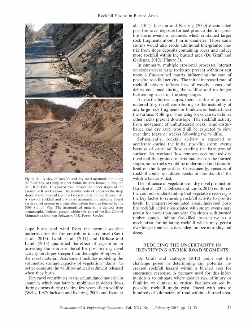
behavior and distances. This reduction in sloperoughness affects whether sufficient momentum isdeveloped to reach a road or facility, and controls thelikelihood that rock slides, rolls, or bounces to acertain height. If the source of rockfall after wildfireswas limited to those rocks previously buttressed bylarge woody debris on the ground surface and thestems of existing shrubs and trees, the hazard posedwould be short-lived (Figure 4). However, loss ofvegetation, consumption of surface organic material,and altering of near-surface soil characteristics alsoinduces dry ravel, a rapid downhill movement ofindividual particles under the influence of gravity notrequiring the presence of water (Swanson, 1981;Florsheim et al., 1991; Gabet, 2003; and Jacksonand Roering, 2009). Dry ravel is a post-fire processdocumented in different parts of the western UnitedStates (Florsheim et al., 1991; Cannon and Reneau,2000; Cannon et al., 2001; and Roering and Gerber,2005).

Movement of fine-grained particles as dry ravel isseen as a primary means for removal of the fine-grained matrix in colluvial, glacial, and fluvialdeposits mantling steep burned slopes, which under-mines support of large rocks on the slope and is asignificant trigger for rockfall. Dry ravel depositsform as cones or aprons of material at the angle ofrepose where natural landscape features like channelsor artificial ones like roads provide a flatter slope(Figure 5a and b). To a degree that is not currentlyquantified, the surface wind generated at the time the

Figure 4. Burned woody plant stems buttressing rocks on theslope above Lumsden Road within the 2013 Rim Fire on theStanislaus National Forest, Sierra Nevada, California. The slopesteepens to the right in this view with the photographer standingon the road. The visibly abundant rock fragments available in thecolluvium mantling this slope can potentially be mobilizedtowards the road during future storm events (Jerome De Graff,U.S. Forest Service).



slope burns and wind from the normal weatherpatterns after the fire contribute to dry ravel (Santiet al., 2013). Lamb et al. (2011) and DiBiase andLamb (2013) quantified the effect of vegetation inproviding the source material for post-fire dry ravelactivity on slopes steeper than the angle of repose forthe ravel material. Assessment includes modeling thevolumetric storage capacity of vegetation ‘‘dams’’ tobetter compute the wildfire-induced sediment releasedwhen they burn.

Dry ravel contributes to the accumulated material inchannels which can later be mobilized in debris flowsduring storms during the first few years after a wildfire(Wells, 1987; Jackson and Roering, 2009; and Kean et

al., 2011). Jackson and Roering (2009) documentedpost-fire ravel deposits formed prior to the first post-fire storm events in channels which contained largerrock fragments about 1 m in diameter. Those samestorms would also erode additional fine-grained ma-trix from slope deposits containing rocks and inducemore rockfall within the burned area (De Graff andGallegos, 2012) (Figure 3).

In summary, multiple erosional processes interacton slopes where large rocks are present within or restupon a fine-grained matrix influencing the rate ofpost-fire rockfall activity. The initial increased rate ofrockfall activity reflects loss of woody stems anddebris consumed during the wildfire and no longerbuttressing rocks on the steep slopes.

Across the burned slopes, there is a flux of granularmaterial (dry ravel) contributing to the instability ofany large rock fragments or boulders embedded nearthe surface. Rolling or bouncing rocks can destabilizeother rocks present downslope. The rockfall activityfrom movement of unbuttressed rocks, wind distur-bance and dry ravel would all be expected to slowover time (days or weeks) following the wildfire.

Subsequently, rockfall activity is expected toaccelerate during the initial post-fire storm eventsbecause of overland flow eroding the bare groundsurface. As overland flow removes accumulated dryravel and fine-grained matrix material on the burnedslopes, some rocks would be undermined and destabi-lized on the slope surface. Consequently, episodes ofrockfall could be induced weeks or months after thewildfire has subsided.

The influence of vegetation on dry ravel production(Lamb et al., 2011; DiBiase and Lamb, 2013) reinforcesthe common understanding that vegetative recovery isthe key factor to returning rockfall activity to pre-firelevels. In chaparral-dominated areas, increased post-fire rockfall activity associated with storm events maypersist for more than one year. On slopes with burnedtimber stands, falling fire-killed trees serve as amechanism for initiating rockfall which may persistover longer time scales dependent on tree mortality anddecay.

REDUCING THE UNCERTAINTY INIDENTIFYING AT-RISK ROAD SEGMENTS

De Graff and Gallegos (2012) point out thechallenge posed in determining any potential in-creased rockfall hazard within a burned area foremergency response. A primary need for this infor-mation is to mitigate where greater risk of injury orfatalities or damage to critical facilities caused bypost-fire rockfall might exist. Faced with tens tohundreds of kilometers of road within a burned area,

Figure 5a. A view of rockfall and dry ravel accumulation alongthe road west of Camp Mather within the area burned during the2013 Rim Fire. This paved road crosses the upper slopes of theTuolumne River Canyon. The granitic bedrock underlies the steepslopes above the road (Jerome De Graff, U.S. Forest Service). 5b.A view of rockfall and dry ravel accumulation along a ForestService road present in a watershed within the area burned by the2009 Station Fire. The accumulated material is derived frommetamorphic bedrock present within this part of the San GabrielMountains (Jonathan Schwartz, U.S. Forest Service).



the uncertainty associated with identifying whichsegments may have a greater rockfall risk is daunting.As mitigation, it is neither practical to close all roadspotentially at risk for an extended period nor effectiveto place hazard warning signs along all roads withinthe fire perimeter having an assumed greater rockfallrisk.

An initial effort was made between 2007 and 2013to identify characteristics useful in identifying roadsegments at higher risk of wildfire-related rockfall. Ageologist experienced in both burned area assessmentand landslide processes participated on teams assem-bled for sixteen wildfires in California during thisperiod. Of the sixteen wildfires, field observationsidentified seven where significant rockfall occurred onroads within days after the slopes above them burned.The eighth rockfall-affected road in this dataset is the

one previously described by the fire managementobserver on the Trinity Ridge wildfire (Figure 6).

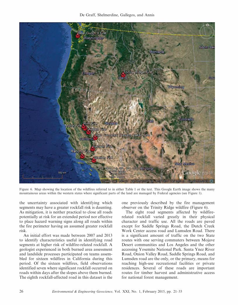
The eight road segments affected by wildfire-related rockfall varied greatly in their physicalcharacter and traffic use. All the roads are pavedexcept for Saddle Springs Road, the Dutch CreekWork Center access road and Lumsden Road. Thereis a significant amount of traffic on the two Stateroutes with one serving commuters between MojaveDesert communities and Los Angeles and the otheraccessing Yosemite National Park. Santa Ynez RiverRoad, Onion Valley Road, Saddle Springs Road, andLumsden road are the only, or the primary, means forreaching high-use recreational facilities or privateresidences. Several of these roads are importantroutes for timber harvest and administrative accessfor national forest management.

Figure 6. Map showing the location of the wildfires referred to in either Table 1 or the text. This Google Earth image shows the manymountainous areas within the western states where significant parts of the land are managed by Federal agencies (see Figure 1).



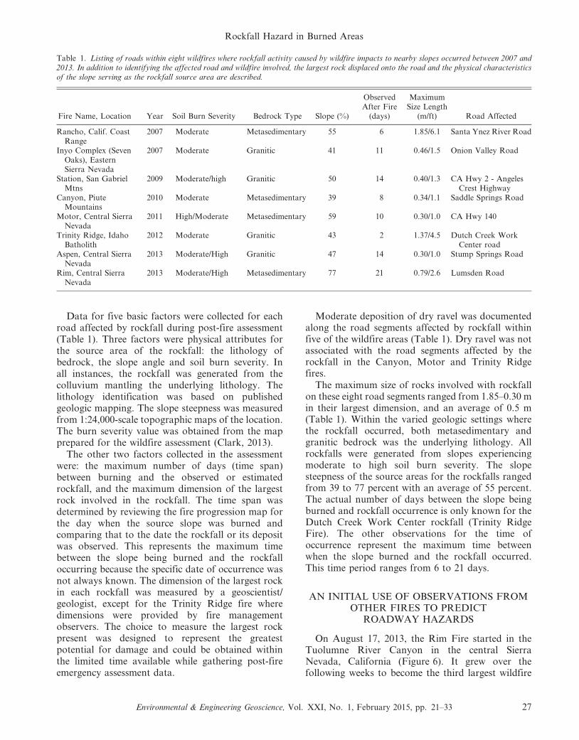
Data for five basic factors were collected for eachroad affected by rockfall during post-fire assessment(Table 1). Three factors were physical attributes forthe source area of the rockfall: the lithology ofbedrock, the slope angle and soil burn severity. Inall instances, the rockfall was generated from thecolluvium mantling the underlying lithology. Thelithology identification was based on publishedgeologic mapping. The slope steepness was measuredfrom 1:24,000-scale topographic maps of the location.The burn severity value was obtained from the mapprepared for the wildfire assessment (Clark, 2013).

The other two factors collected in the assessmentwere: the maximum number of days (time span)between burning and the observed or estimatedrockfall, and the maximum dimension of the largestrock involved in the rockfall. The time span wasdetermined by reviewing the fire progression map forthe day when the source slope was burned andcomparing that to the date the rockfall or its depositwas observed. This represents the maximum timebetween the slope being burned and the rockfalloccurring because the specific date of occurrence wasnot always known. The dimension of the largest rockin each rockfall was measured by a geoscientist/geologist, except for the Trinity Ridge fire wheredimensions were provided by fire managementobservers. The choice to measure the largest rockpresent was designed to represent the greatestpotential for damage and could be obtained withinthe limited time available while gathering post-fireemergency assessment data.

Moderate deposition of dry ravel was documentedalong the road segments affected by rockfall withinfive of the wildfire areas (Table 1). Dry ravel was notassociated with the road segments affected by therockfall in the Canyon, Motor and Trinity Ridgefires.

The maximum size of rocks involved with rockfallon these eight road segments ranged from 1.85–0.30 min their largest dimension, and an average of 0.5 m(Table 1). Within the varied geologic settings wherethe rockfall occurred, both metasedimentary andgranitic bedrock was the underlying lithology. Allrockfalls were generated from slopes experiencingmoderate to high soil burn severity. The slopesteepness of the source areas for the rockfalls rangedfrom 39 to 77 percent with an average of 55 percent.The actual number of days between the slope beingburned and rockfall occurrence is only known for theDutch Creek Work Center rockfall (Trinity RidgeFire). The other observations for the time ofoccurrence represent the maximum time betweenwhen the slope burned and the rockfall occurred.This time period ranges from 6 to 21 days.

AN INITIAL USE OF OBSERVATIONS FROMOTHER FIRES TO PREDICT

ROADWAY HAZARDS

On August 17, 2013, the Rim Fire started in theTuolumne River Canyon in the central SierraNevada, California (Figure 6). It grew over thefollowing weeks to become the third largest wildfire

Table 1. Listing of roads within eight wildfires where rockfall activity caused by wildfire impacts to nearby slopes occurred between 2007 and2013. In addition to identifying the affected road and wildfire involved, the largest rock displaced onto the road and the physical characteristicsof the slope serving as the rockfall source area are described.

Fire Name, Location Year Soil Burn Severity Bedrock Type Slope (%)

ObservedAfter Fire

(days)

MaximumSize Length

(m/ft) Road Affected

Rancho, Calif. CoastRange

2007 Moderate Metasedimentary 55 6 1.85/6.1 Santa Ynez River Road

Inyo Complex (SevenOaks), EasternSierra Nevada

2007 Moderate Granitic 41 11 0.46/1.5 Onion Valley Road

Station, San GabrielMtns

2009 Moderate/high Granitic 50 14 0.40/1.3 CA Hwy 2 - AngelesCrest Highway

Canyon, PiuteMountains

2010 Moderate Metasedimentary 39 8 0.34/1.1 Saddle Springs Road

Motor, Central SierraNevada

2011 High/Moderate Metasedimentary 59 10 0.30/1.0 CA Hwy 140

Trinity Ridge, IdahoBatholith

2012 Moderate Granitic 43 2 1.37/4.5 Dutch Creek WorkCenter road

Aspen, Central SierraNevada

2013 Moderate/High Granitic 47 14 0.30/1.0 Stump Springs Road

Rim, Central SierraNevada

2013 Moderate/High Metasedimentary 77 21 0.79/2.6 Lumsden Road



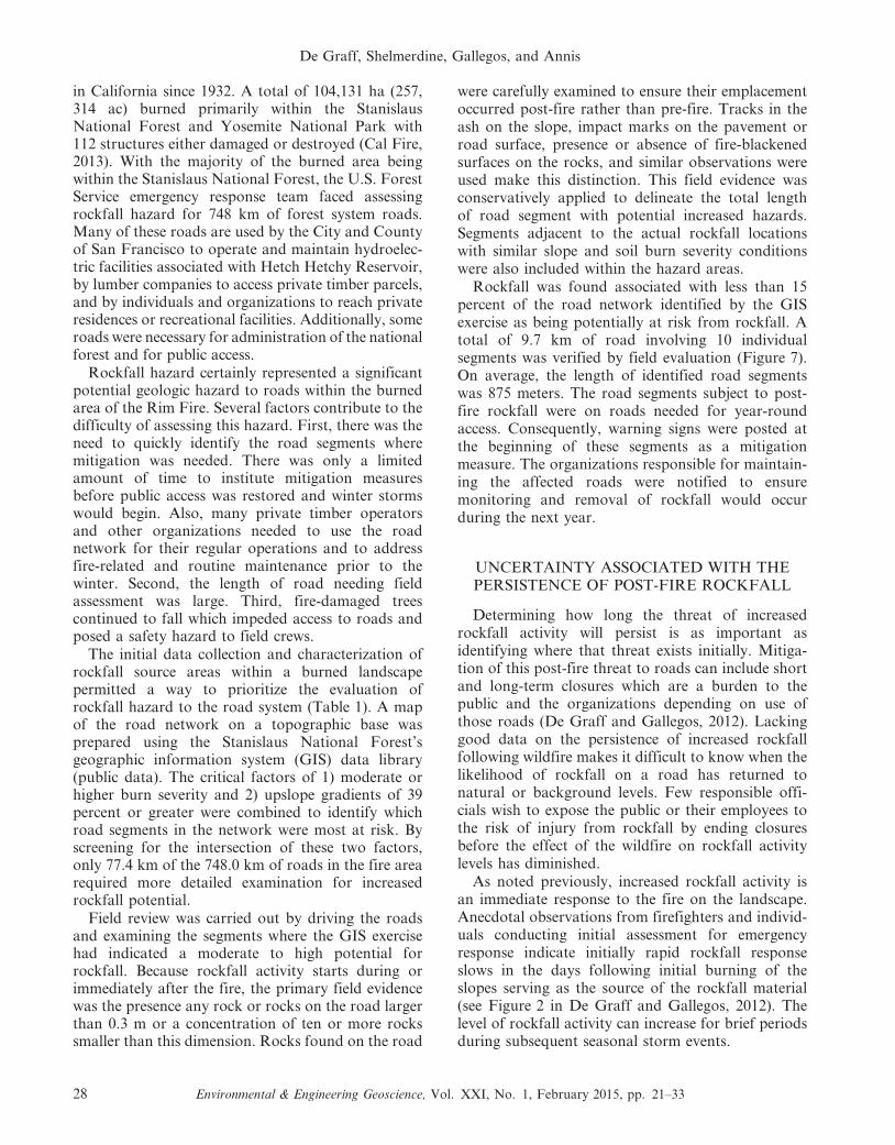
in California since 1932. A total of 104,131 ha (257,314 ac) burned primarily within the StanislausNational Forest and Yosemite National Park with112 structures either damaged or destroyed (Cal Fire,2013). With the majority of the burned area beingwithin the Stanislaus National Forest, the U.S. ForestService emergency response team faced assessingrockfall hazard for 748 km of forest system roads.Many of these roads are used by the City and Countyof San Francisco to operate and maintain hydroelec-tric facilities associated with Hetch Hetchy Reservoir,by lumber companies to access private timber parcels,and by individuals and organizations to reach privateresidences or recreational facilities. Additionally, someroads were necessary for administration of the nationalforest and for public access.

Rockfall hazard certainly represented a significantpotential geologic hazard to roads within the burnedarea of the Rim Fire. Several factors contribute to thedifficulty of assessing this hazard. First, there was theneed to quickly identify the road segments wheremitigation was needed. There was only a limitedamount of time to institute mitigation measuresbefore public access was restored and winter stormswould begin. Also, many private timber operatorsand other organizations needed to use the roadnetwork for their regular operations and to addressfire-related and routine maintenance prior to thewinter. Second, the length of road needing fieldassessment was large. Third, fire-damaged treescontinued to fall which impeded access to roads andposed a safety hazard to field crews.

The initial data collection and characterization ofrockfall source areas within a burned landscapepermitted a way to prioritize the evaluation ofrockfall hazard to the road system (Table 1). A mapof the road network on a topographic base wasprepared using the Stanislaus National Forest’sgeographic information system (GIS) data library(public data). The critical factors of 1) moderate orhigher burn severity and 2) upslope gradients of 39percent or greater were combined to identify whichroad segments in the network were most at risk. Byscreening for the intersection of these two factors,only 77.4 km of the 748.0 km of roads in the fire arearequired more detailed examination for increasedrockfall potential.

Field review was carried out by driving the roadsand examining the segments where the GIS exercisehad indicated a moderate to high potential forrockfall. Because rockfall activity starts during orimmediately after the fire, the primary field evidencewas the presence any rock or rocks on the road largerthan 0.3 m or a concentration of ten or more rockssmaller than this dimension. Rocks found on the road

were carefully examined to ensure their emplacementoccurred post-fire rather than pre-fire. Tracks in theash on the slope, impact marks on the pavement orroad surface, presence or absence of fire-blackenedsurfaces on the rocks, and similar observations wereused make this distinction. This field evidence wasconservatively applied to delineate the total lengthof road segment with potential increased hazards.Segments adjacent to the actual rockfall locationswith similar slope and soil burn severity conditionswere also included within the hazard areas.

Rockfall was found associated with less than 15percent of the road network identified by the GISexercise as being potentially at risk from rockfall. Atotal of 9.7 km of road involving 10 individualsegments was verified by field evaluation (Figure 7).On average, the length of identified road segmentswas 875 meters. The road segments subject to post-fire rockfall were on roads needed for year-roundaccess. Consequently, warning signs were posted atthe beginning of these segments as a mitigationmeasure. The organizations responsible for maintain-ing the affected roads were notified to ensuremonitoring and removal of rockfall would occurduring the next year.

UNCERTAINTY ASSOCIATED WITH THEPERSISTENCE OF POST-FIRE ROCKFALL

Determining how long the threat of increasedrockfall activity will persist is as important asidentifying where that threat exists initially. Mitiga-tion of this post-fire threat to roads can include shortand long-term closures which are a burden to thepublic and the organizations depending on use ofthose roads (De Graff and Gallegos, 2012). Lackinggood data on the persistence of increased rockfallfollowing wildfire makes it difficult to know when thelikelihood of rockfall on a road has returned tonatural or background levels. Few responsible offi-cials wish to expose the public or their employees tothe risk of injury from rockfall by ending closuresbefore the effect of the wildfire on rockfall activitylevels has diminished.

As noted previously, increased rockfall activity isan immediate response to the fire on the landscape.Anecdotal observations from firefighters and individ-uals conducting initial assessment for emergencyresponse indicate initially rapid rockfall responseslows in the days following initial burning of theslopes serving as the source of the rockfall material(see Figure 2 in De Graff and Gallegos, 2012). Thelevel of rockfall activity can increase for brief periodsduring subsequent seasonal storm events.



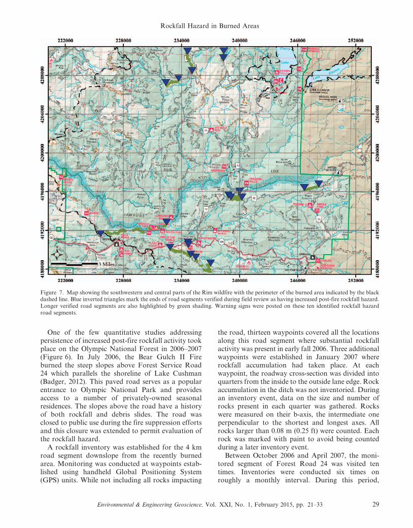
One of the few quantitative studies addressingpersistence of increased post-fire rockfall activity tookplace on the Olympic National Forest in 2006–2007(Figure 6). In July 2006, the Bear Gulch II Fireburned the steep slopes above Forest Service Road24 which parallels the shoreline of Lake Cushman(Badger, 2012). This paved road serves as a popularentrance to Olympic National Park and providesaccess to a number of privately-owned seasonalresidences. The slopes above the road have a historyof both rockfall and debris slides. The road wasclosed to public use during the fire suppression effortsand this closure was extended to permit evaluation ofthe rockfall hazard.

A rockfall inventory was established for the 4 kmroad segment downslope from the recently burnedarea. Monitoring was conducted at waypoints estab-lished using handheld Global Positioning System(GPS) units. While not including all rocks impacting

the road, thirteen waypoints covered all the locationsalong this road segment where substantial rockfallactivity was present in early fall 2006. Three additionalwaypoints were established in January 2007 whererockfall accumulation had taken place. At eachwaypoint, the roadway cross-section was divided intoquarters from the inside to the outside lane edge. Rockaccumulation in the ditch was not inventoried. Duringan inventory event, data on the size and number ofrocks present in each quarter was gathered. Rockswere measured on their b-axis, the intermediate oneperpendicular to the shortest and longest axes. Allrocks larger than 0.08 m (0.25 ft) were counted. Eachrock was marked with paint to avoid being countedduring a later inventory event.

Between October 2006 and April 2007, the moni-tored segment of Forest Road 24 was visited tentimes. Inventories were conducted six times onroughly a monthly interval. During this period,

Figure 7. Map showing the southwestern and central parts of the Rim wildfire with the perimeter of the burned area indicated by the blackdashed line. Blue inverted triangles mark the ends of road segments verified during field review as having increased post-fire rockfall hazard.Longer verified road segments are also highlighted by green shading. Warning signs were posted on these ten identified rockfall hazardroad segments.



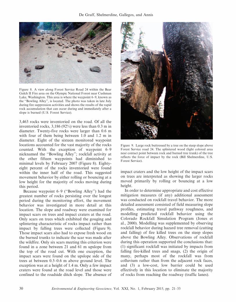
3,463 rocks were inventoried on the road. Of all theinventoried rocks, 3,186 (92%) were less than 0.3 m indiameter. Twenty-five rocks were larger than 0.6 mwith four of them being between 1.0 and 1.2 m indiameter. Eight of the sixteen monitored waypointlocations accounted for the vast majority of the rockscounted. With the exception of waypoint 6–9nicknamed the ‘‘Bowling Alley’’; rockfall activity atthe other fifteen waypoints had diminished tominimal levels by February 2007 (Figure 8). Eighty-eight percent of the rocks inventoried were foundwithin the inner half of the road. This suggestedmovement behavior by either rolling or bouncing at alow height for the majority of rocks moving duringthis period.

Because waypoint 6–9 (‘‘Bowling Alley’’) had thegreatest number of rocks persisting over the longestperiod during the monitoring effort, the movementbehavior was investigated in more detail at thislocation. The slope and roadway were examined forimpact scars on trees and impact craters at the road.Only scars on trees which exhibited the gouging andsplintering characteristic of rocks impact rather thanimpact by falling trees were collected (Figure 9).Those impact scars also had to expose fresh wood onthe burned trunks to indicate the scar was made afterthe wildfire. Only six scars meeting this criterion werefound in a zone between 21 and 61 m upslope fromthe top of the road cut. With one exception, theimpact scars were found on the upslope side of thetrees at between 0.5–0.6 m above ground level. Theexception was at a height of 1.4 m. Only a few impactcraters were found at the road level and those wereconfined to the roadside ditch slope. The absence of

impact craters and the low height of the impact scarson trees are interpreted as showing the larger rocksmoved primarily by rolling or bouncing at a lowheight.

In order to determine appropriate and cost effectivemitigation measures (if any) additional assessmentwas conducted on rockfall travel behavior. The moredetailed assessment consisted of field measuring slopeprofiles, estimating travel pathway roughness, andmodelling predicted rockfall behavior using theColorado Rockfall Simulation Program (Jones etal., 2000). Modelling was supplemented by observingrockfall behavior during hazard tree removal (cuttingand falling) of fire killed trees on the steep slopesabove the Bowling Alley. Observations of rockfallduring this operation supported the conclusions that:(1) significant rockfall was initiated by impacts fromfalling fire-killed trees and snags, (2) the origin ofmany, perhaps most of the rockfall was fromcolluvium rather than from the adjacent rock faces,and (3) a low-cost, low barrier could be usedeffectively in this location to eliminate the majorityof rocks from reaching the roadway (traffic lanes).

Figure 8. A view along Forest Service Road 24 within the BearGulch II Fire area on the Olympic National Forest near CushmanLake, Washington. This area is where the waypoint 6–9, known asthe ‘‘Bowling Alley’’, is located. The photo was taken in late Julyduring fire suppression activities and shows the results of the rapidrock accumulation that can occur during and immediately after aslope is burned (U.S. Forest Service).

Figure 9. Large rock buttressed by a tree on the steep slope aboveForest Service road 24. The splintered wood (light colored areanear contact point between rock and burned tree trunk) of the treereflects the force of impact by the rock (Bill Shelmerdine, U.S.Forest Service).



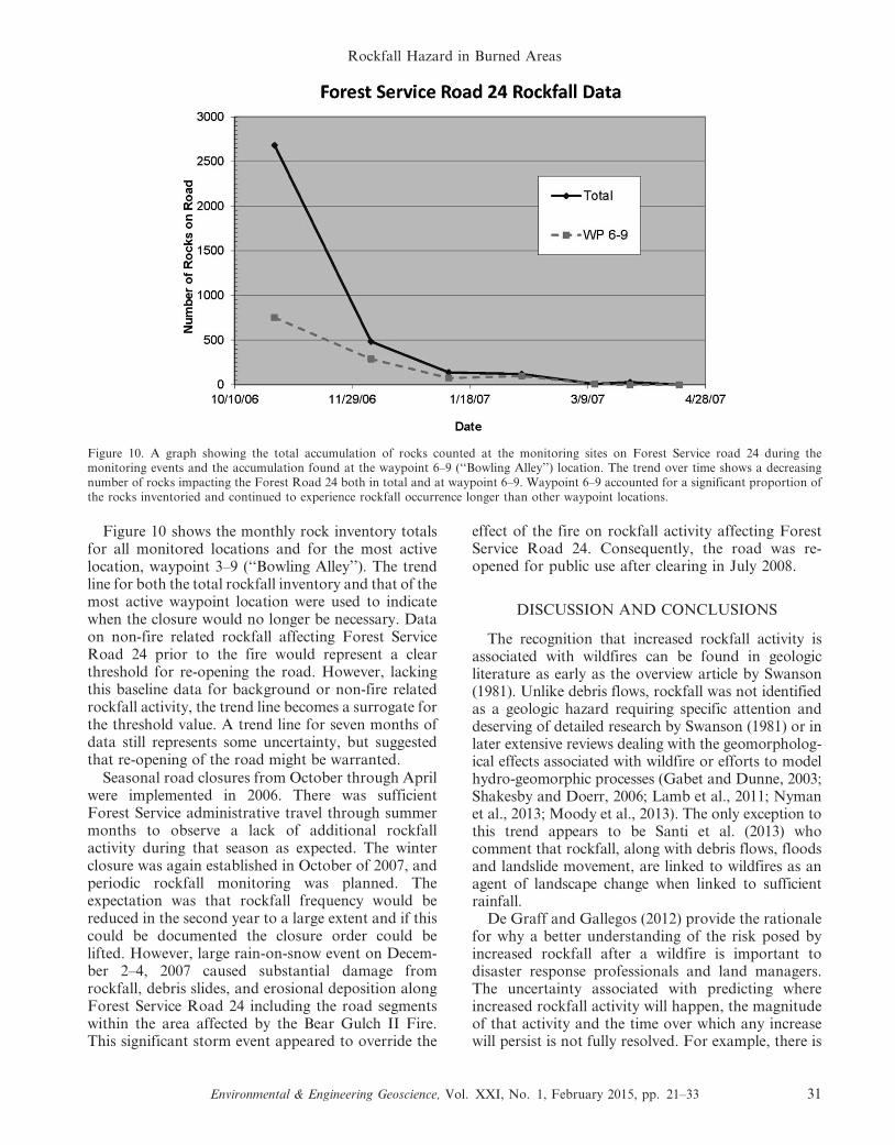
Figure 10 shows the monthly rock inventory totalsfor all monitored locations and for the most activelocation, waypoint 3–9 (‘‘Bowling Alley’’). The trendline for both the total rockfall inventory and that of themost active waypoint location were used to indicatewhen the closure would no longer be necessary. Dataon non-fire related rockfall affecting Forest ServiceRoad 24 prior to the fire would represent a clearthreshold for re-opening the road. However, lackingthis baseline data for background or non-fire relatedrockfall activity, the trend line becomes a surrogate forthe threshold value. A trend line for seven months ofdata still represents some uncertainty, but suggestedthat re-opening of the road might be warranted.

Seasonal road closures from October through Aprilwere implemented in 2006. There was sufficientForest Service administrative travel through summermonths to observe a lack of additional rockfallactivity during that season as expected. The winterclosure was again established in October of 2007, andperiodic rockfall monitoring was planned. Theexpectation was that rockfall frequency would bereduced in the second year to a large extent and if thiscould be documented the closure order could belifted. However, large rain-on-snow event on Decem-ber 2–4, 2007 caused substantial damage fromrockfall, debris slides, and erosional deposition alongForest Service Road 24 including the road segmentswithin the area affected by the Bear Gulch II Fire.This significant storm event appeared to override the

effect of the fire on rockfall activity affecting ForestService Road 24. Consequently, the road was re-opened for public use after clearing in July 2008.

DISCUSSION AND CONCLUSIONS

The recognition that increased rockfall activity isassociated with wildfires can be found in geologicliterature as early as the overview article by Swanson(1981). Unlike debris flows, rockfall was not identifiedas a geologic hazard requiring specific attention anddeserving of detailed research by Swanson (1981) or inlater extensive reviews dealing with the geomorpholog-ical effects associated with wildfire or efforts to modelhydro-geomorphic processes (Gabet and Dunne, 2003;Shakesby and Doerr, 2006; Lamb et al., 2011; Nymanet al., 2013; Moody et al., 2013). The only exception tothis trend appears to be Santi et al. (2013) whocomment that rockfall, along with debris flows, floodsand landslide movement, are linked to wildfires as anagent of landscape change when linked to sufficientrainfall.

De Graff and Gallegos (2012) provide the rationalefor why a better understanding of the risk posed byincreased rockfall after a wildfire is important todisaster response professionals and land managers.The uncertainty associated with predicting whereincreased rockfall activity will happen, the magnitudeof that activity and the time over which any increasewill persist is not fully resolved. For example, there is

Figure 10. A graph showing the total accumulation of rocks counted at the monitoring sites on Forest Service road 24 during themonitoring events and the accumulation found at the waypoint 6–9 (‘‘Bowling Alley’’) location. The trend over time shows a decreasingnumber of rocks impacting the Forest Road 24 both in total and at waypoint 6–9. Waypoint 6–9 accounted for a significant proportion ofthe rocks inventoried and continued to experience rockfall occurrence longer than other waypoint locations.



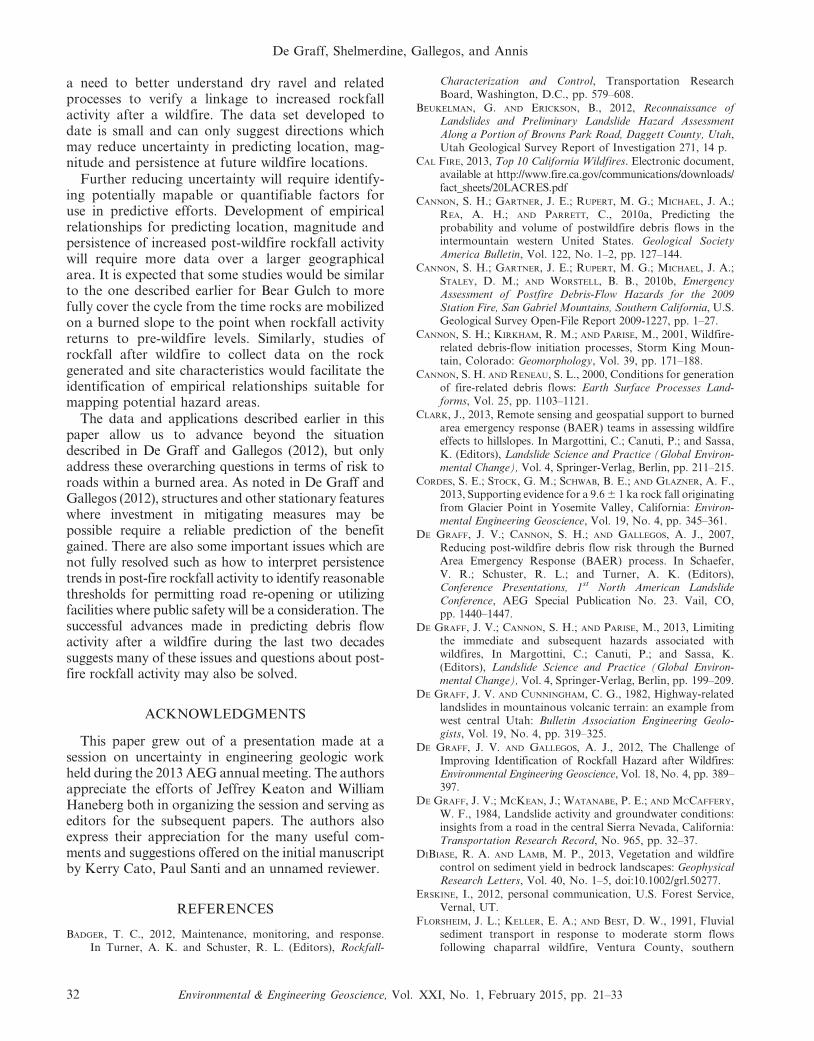
a need to better understand dry ravel and relatedprocesses to verify a linkage to increased rockfallactivity after a wildfire. The data set developed todate is small and can only suggest directions whichmay reduce uncertainty in predicting location, mag-nitude and persistence at future wildfire locations.

Further reducing uncertainty will require identify-ing potentially mapable or quantifiable factors foruse in predictive efforts. Development of empiricalrelationships for predicting location, magnitude andpersistence of increased post-wildfire rockfall activitywill require more data over a larger geographicalarea. It is expected that some studies would be similarto the one described earlier for Bear Gulch to morefully cover the cycle from the time rocks are mobilizedon a burned slope to the point when rockfall activityreturns to pre-wildfire levels. Similarly, studies ofrockfall after wildfire to collect data on the rockgenerated and site characteristics would facilitate theidentification of empirical relationships suitable formapping potential hazard areas.

The data and applications described earlier in thispaper allow us to advance beyond the situationdescribed in De Graff and Gallegos (2012), but onlyaddress these overarching questions in terms of risk toroads within a burned area. As noted in De Graff andGallegos (2012), structures and other stationary featureswhere investment in mitigating measures may bepossible require a reliable prediction of the benefitgained. There are also some important issues which arenot fully resolved such as how to interpret persistencetrends in post-fire rockfall activity to identify reasonablethresholds for permitting road re-opening or utilizingfacilities where public safety will be a consideration. Thesuccessful advances made in predicting debris flowactivity after a wildfire during the last two decadessuggests many of these issues and questions about post-fire rockfall activity may also be solved.

ACKNOWLEDGMENTS

This paper grew out of a presentation made at asession on uncertainty in engineering geologic workheld during the 2013 AEG annual meeting. The authorsappreciate the efforts of Jeffrey Keaton and WilliamHaneberg both in organizing the session and serving aseditors for the subsequent papers. The authors alsoexpress their appreciation for the many useful com-ments and suggestions offered on the initial manuscriptby Kerry Cato, Paul Santi and an unnamed reviewer.

REFERENCES

BADGER, T. C., 2012, Maintenance, monitoring, and response.In Turner, A. K. and Schuster, R. L. (Editors), Rockfall-

Characterization and Control, Transportation ResearchBoard, Washington, D.C., pp. 579–608.

BEUKELMAN, G. AND ERICKSON, B., 2012, Reconnaissance ofLandslides and Preliminary Landslide Hazard AssessmentAlong a Portion of Browns Park Road, Daggett County, Utah,Utah Geological Survey Report of Investigation 271, 14 p.

CAL FIRE, 2013, Top 10 California Wildfires. Electronic document,available at http://www.fire.ca.gov/communications/downloads/fact_sheets/20LACRES.pdf

CANNON, S. H.; GARTNER, J. E.; RUPERT, M. G.; MICHAEL, J. A.;REA, A. H.; AND PARRETT, C., 2010a, Predicting theprobability and volume of postwildfire debris flows in theintermountain western United States. Geological SocietyAmerica Bulletin, Vol. 122, No. 1–2, pp. 127–144.

CANNON, S. H.; GARTNER, J. E.; RUPERT, M. G.; MICHAEL, J. A.;STALEY, D. M.; AND WORSTELL, B. B., 2010b, EmergencyAssessment of Postfire Debris-Flow Hazards for the 2009Station Fire, San Gabriel Mountains, Southern California, U.S.Geological Survey Open-File Report 2009-1227, pp. 1–27.

CANNON, S. H.; KIRKHAM, R. M.; AND PARISE, M., 2001, Wildfire-related debris-flow initiation processes, Storm King Moun-tain, Colorado: Geomorphology, Vol. 39, pp. 171–188.

CANNON, S. H. AND RENEAU, S. L., 2000, Conditions for generationof fire-related debris flows: Earth Surface Processes Land-forms, Vol. 25, pp. 1103–1121.

CLARK, J., 2013, Remote sensing and geospatial support to burnedarea emergency response (BAER) teams in assessing wildfireeffects to hillslopes. In Margottini, C.; Canuti, P.; and Sassa,K. (Editors), Landslide Science and Practice (Global Environ-mental Change), Vol. 4, Springer-Verlag, Berlin, pp. 211–215.

CORDES, S. E.; STOCK, G. M.; SCHWAB, B. E.; AND GLAZNER, A. F.,2013, Supporting evidence for a 9.6 6 1 ka rock fall originatingfrom Glacier Point in Yosemite Valley, California: Environ-mental Engineering Geoscience, Vol. 19, No. 4, pp. 345–361.

DE GRAFF, J. V.; CANNON, S. H.; AND GALLEGOS, A. J., 2007,Reducing post-wildfire debris flow risk through the BurnedArea Emergency Response (BAER) process. In Schaefer,V. R.; Schuster, R. L.; and Turner, A. K. (Editors),Conference Presentations, 1st North American LandslideConference, AEG Special Publication No. 23. Vail, CO,pp. 1440–1447.

DE GRAFF, J. V.; CANNON, S. H.; AND PARISE, M., 2013, Limitingthe immediate and subsequent hazards associated withwildfires, In Margottini, C.; Canuti, P.; and Sassa, K.(Editors), Landslide Science and Practice (Global Environ-mental Change), Vol. 4, Springer-Verlag, Berlin, pp. 199–209.

DE GRAFF, J. V. AND CUNNINGHAM, C. G., 1982, Highway-relatedlandslides in mountainous volcanic terrain: an example fromwest central Utah: Bulletin Association Engineering Geolo-gists, Vol. 19, No. 4, pp. 319–325.

DE GRAFF, J. V. AND GALLEGOS, A. J., 2012, The Challenge ofImproving Identification of Rockfall Hazard after Wildfires:Environmental Engineering Geoscience, Vol. 18, No. 4, pp. 389–397.

DE GRAFF, J. V.; MCKEAN, J.; WATANABE, P. E.; AND MCCAFFERY,W. F., 1984, Landslide activity and groundwater conditions:insights from a road in the central Sierra Nevada, California:Transportation Research Record, No. 965, pp. 32–37.

DIBIASE, R. A. AND LAMB, M. P., 2013, Vegetation and wildfirecontrol on sediment yield in bedrock landscapes: GeophysicalResearch Letters, Vol. 40, No. 1–5, doi:10.1002/grl.50277.

ERSKINE, I., 2012, personal communication, U.S. Forest Service,Vernal, UT.

FLORSHEIM, J. L.; KELLER, E. A.; AND BEST, D. W., 1991, Fluvialsediment transport in response to moderate storm flowsfollowing chaparral wildfire, Ventura County, southern



California. Geological Society America Bulletin, Vol. 103,pp. 504–511.

GABET, E. J., 2003, Sediment transport by dry ravel: JournalGeophysical Research: Solid Earth (1978–2012), Vol. 108,Issue B1, pp: 2049, doi: 10.1029/2001JB001686

GABET, E. J. AND DUNNE, T., 2003, A stochastic sediment deliverymodel for a steep Mediterranean landscape: Water ResourcesResearch, Vol. 39, No. 9, pp: 1237, doi: 10.1029/2003WRR002341

HARP, E. L.; REID, M. E.; GODT, J. W.; DE GRAFF, J. V.; AND

GALLEGOS, A. J., 2008, Ferguson rock slide buries CaliforniaState Highway near Yosemite National Park: Landslides,Vol. 5, No. 3, pp. 331–337.

JACKSON, M. AND ROERING, J. J., 2009, Post-fire geomorphicresponse in steep, forested landscapes: Oregon Coast Range,USA: Quaternary Science Reviews, Vol. 28, No. 11–12, pp.1131–1146.

JONES, C. L.; HIGGINS, J. D.; AND ANDREW, R. D., 2000, Coloradorockfall simulation program version 4.0. Colorado Depart-ment of Transportation, Colorado Geological Survey,Denver, CO, 127 p.

KEAN, J. W.; STALEY, D. M.; AND CANNON, S. H., 2011, In situmeasurements of post-fire debris flows in southern Califor-nia: Comparisons of the timing and magnitude of 24 debris-flow events with rainfall and soil moisture conditions: JournalGeophysical Research, Vol. 116, No. F4, p. F04019.

LAMB, M. P.; SCHEINGROSS, J. S.; AMIDON, W. H.; SWANSON, E.;AND LIMAYE, A., 2011, A model for fire-induced sedimentyield by dry ravel in steep landscapes: Journal GeophysicalResearch 116, F03006, doi: 10.1029/2010JF001878

LEBLANC, R., 2013 personal communication, Stanislaus NF RoadsEngineer, Sonora, CA.

LEMMON, M., 2011 personal communication, Motor Fire IncidentCommander, Clovis, CA.

LITTELL, J. S.; MCKENZIE, D.; PETERSON, D. L.; AND WESTERLING,A. L., 2009, Climate and wildfire burned in western U.S.Ecoprovinces, 1916–2003: Ecological Applications, Vol. 19,No. 4, pp. 1003–1021.

MOODY, J. A.; SHAKESBY, R. A.; ROBICHAUD, P. R.; CANNON, S. H.;AND MARTIN, D. A., 2013, Current research issues related topost-wildfire runoff and erosion processes: Earth ScienceReviews, doi: 10.1016/j.earscirev.2013.03.004

NYMAN, P.; SHERIDAN, G. L.; AND LANE, P. N. J., 2013, Hydro-

geomorphic response models for burned areas and their

applications in land management: Progress Physical Geogra-

phy, Vol. 37, No. 6, pp. 787–812.

PARSONS, A.; ROBICHAUD, P. R.; LEWIS, S. A.; NAPPER, C.; AND

CLARK, J. T., 2010, Field Guide for Mapping Post-fire Soil

Burn Severity, USDA Forest Service General Technical

Report RMRS-GR-243, 49 p.

ROERING, J. J. AND GERBER, M., 2005, Fire and the evolution of

steep, soil-mantled landscapes: Geology, Vol. 33, No. 5,

pp. 349–352.

SANTI, P.; CANNON, S.; AND DE GRAFF, J., 2013, Wildfire and

Landscape Change, In Shroder, J. F. (Editor), Treatise

Geomorphology, Vol. 13, Academic Press, San Diego,

pp. 262–287.

SHAKESBY, R. A. AND DOERR, S. H., 2006, Wildfire as a

hydrological and geomorphological agent. Earth-Science

Reviews, Vol. 74, pp. 269–307.

STEPHENS, S. L., 2005, Forest fire causes and extent on United

States Forest Service lands: International Journal Wildland

Fire, Vol. 14, pp. 213–222.

SWANSON, F. J., 1981, Fire and geomorphic processes. In Mooney,

H. A.; Bonnicksen, T. M.; Christensen, N. L.; Lotan, J. E.;

and Reiners, W. A. (Editors), Fire Regime and Ecosystem

Properties, pp. 401–421. USDA Forest Service General

Technical Report WO-26.

TURNER, A. K. AND JAYPRAKASH, G. P., 2012, Introduction, In

Turner, A. K. and Schuster, R. L. (Editors), Rockfall-

Characterization and Control, Transportation Research

Board, Washington, D.C., pp. 3–20.

VARNES, D. J., 1978, Slope movement types and processes. In

Schuster, R. L. and Krizek, R. J. (Editors), Landslide

Analysis and Control, Transportation Research Board,

Washington, DC, pp. 11–33.

WELLS, W. G., 1987, The effects of fire on the generation of debris

flows in southern California. Reviews Engineering Geology,

Vol. 7, pp. 105–114.

WESTERLING, A. L.; HIDALGO, H. G.; CAYAN, D. R.; AND SWETNAM,

T. W., 2006, Warming and earlier spring increase U.S. Forest

wildfire activity: Science, Vol. 313, pp. 940–943.



Complex Landslide Triggered in an Eocene

Volcanic-Volcaniclastic Succession along Sutherland

River, British Columbia, Canada

ANDREE BLAIS-STEVENS1

Geological Survey of Canada, 601 Booth Street, Ottawa, Ontario, K1A 0E8

MARTEN GEERTSEMA

BC Ministry of Forests, Lands, and Natural Resource Operations,1044 5th Avenue, Prince George, British Columbia V2L 5G4

JAMES W. SCHWAB

P.O. Box 2525, Smithers, British Columbia V0J 2N0

THEO W. J. VAN ASCH

Department of Physical Geography, Utrecht University, P.O. Box 80115,3508 TC Utrecht, The Netherlands

Key Terms: Northern British Columbia, Landslide,Complex Rock slide-Debris Avalanche, Seismic Signal,Eocene Volcanic and Volcaniclastic Rocks

ABSTRACT

On July 13, 2005 a complex 3 Mm3 and 1.5 km longrock slide-debris avalanche occurred near SutherlandRiver, 40 km west of Fort St. James, British Columbia,Canada. The landslide was initiated in a succession ofsub-horizontal competent mafic basalts (Endako For-mation) capping weaker felsic volcanic and volcaniclas-tic rocks (Ootsa Lake Group) of Eocene age. Severallandslides have been observed in similar volcanicsuccessions worldwide including in southern BritishColumbia. Some common characteristics of theselandslides are: structurally undisturbed; horizontal tosub-horizontal bedding; curved head scarp; steep joints;debris consists of intact blocks; volcaniclastics contain-ing smectite (expandable clay mineral); fossils andlignite within the volcaniclastics. The Sutherlandlandslide is one of many large landslides that haveoccurred in recent years in northern British Columbia.At least eight other large landslides have been triggeredin volcanic rocks within the Nechako plateau.

INTRODUCTION

On the southwestern flank of the Sutherland Rivervalley, approximately 40 km west of Fort St. James,within Sutherland River Provincial Park, located in anisolated area of north central British Columbia (BC) isthe Sutherland complex landslide; a rock slide-debrisavalanche (Blais-Stevens et al., 2007; Figure 1). Thislarge 3 Mm3 complex landslide was initiated in Eocenevolcanics and volcaniclastics on the Nechako Plateau(Struik et al., 2000). It destroyed an estimated area of40 ha with an approximate volume of 8,000 m3 oftimber. Air photos dated as far back as 1957 indicate thehead scarp had experienced on-going deformation. Theobjectives of the paper are to expand on preliminaryresults from research by Blais-Stevens et al. (2007) anddescribe the Sutherland landslide setting and landslidepre-conditions in an attempt to understand the potentialtriggers, characteristics, material properties, and slopemovement. A comparison is made with other large rockslides in northern BC as well as some that have occurredin similar volcanic successions in southern BC andworldwide. Natural gas and oil pipelines are projectedto cross the Nechako Plateau’s subdued topography.Thus, identification of potential landslide zones in thistype of terrain will help decision-makers in assessing thelandslide risk to infrastructure and population.

PHYSIOGRAPHIC AND GEOLOGIC SETTING

The Nechako Plateau physiographic region, wherethe Sutherland landslide is located, is part of the1Corresponding author email: [email protected].


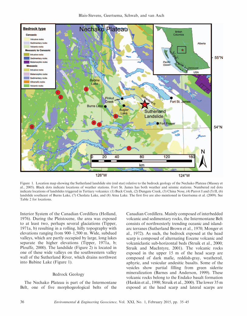
Interior System of the Canadian Cordillera (Holland,1976). During the Pleistocene, the area was exposedto at least two, perhaps several glaciations (Tipper,1971a, b) resulting in a rolling, hilly topography withelevations ranging from 900–1,500 m. Wide, subduedvalleys, which are partly occupied by large, long lakesseparate the higher elevations (Tipper, 1971a, b;Plouffe, 2000). The landslide (Figure 2) is located inone of these wide valleys on the southwestern valleywall of the Sutherland River, which drains northwestinto Babine Lake (Figure 1).

Bedrock Geology

The Nechako Plateau is part of the IntermontaneBelt, one of five morphogeological belts of the

Canadian Cordillera. Mainly composed of interbeddedvolcanic and sedimentary rocks, the Intermontane Beltconsists of northwesterly trending oceanic and island-arc terranes (Sutherland Brown et al., 1970; Monger etal., 1972). As such, the bedrock exposed at the headscarp is composed of alternating Eocene volcanic andvolcaniclastic sub-horizontal beds (Struik et al., 2000;Struik and MacIntyre, 2001). The volcanic rocksexposed in the upper 15 m of the head scarp arecomposed of dark mafic, reddish-gray, weathered,aphyric, and vesicular andesitic basalts. Some of thevesicles show partial filling from green sideritemineralization (Barnes and Anderson, 1999). Thesevolcanic rocks belong to the Endako basalt formation(Haskin et al., 1998; Struik et al., 2000). The lower 35 mexposed at the head scarp and lateral scarps are

Figure 1. Location map showing the Sutherland landslide site (red star) relative to the bedrock geology of the Nechako Plateau (Massey etal., 2005). Black dots indicate locations of weather stations. Fort St. James has both weather and seismic stations. Numbered red dotsindicate locations of landslides triggered in Tertiary volcanics: (1) Buck Creek, (2) Dungate Creek, (3) China Nose, (4) Parrot I and (5) II, (6)landslide southeast of Burns Lake, (7) Cheslata Lake, and (8) Atna Lake. The first five are also mentioned in Geertsema et al. (2009). SeeTable 2 for locations.

Blais-Stevens, Geertsema, Schwab, and van Asch


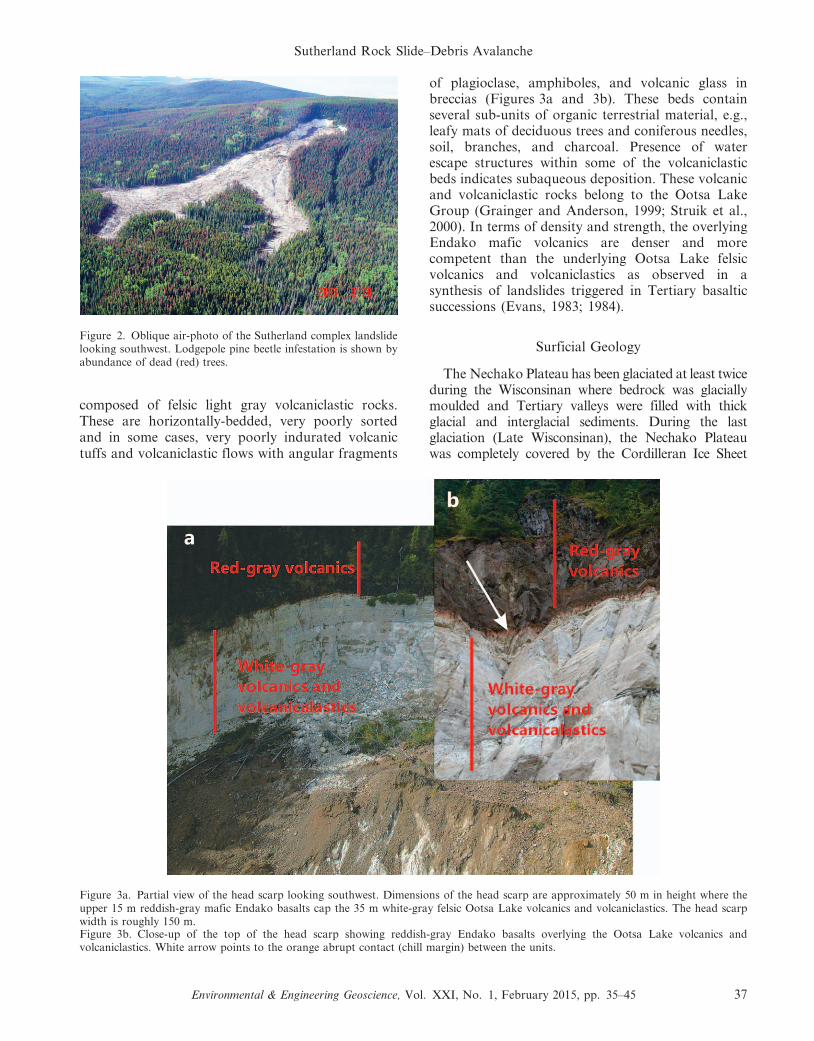
composed of felsic light gray volcaniclastic rocks.These are horizontally-bedded, very poorly sortedand in some cases, very poorly indurated volcanictuffs and volcaniclastic flows with angular fragments

of plagioclase, amphiboles, and volcanic glass inbreccias (Figures 3a and 3b). These beds containseveral sub-units of organic terrestrial material, e.g.,leafy mats of deciduous trees and coniferous needles,soil, branches, and charcoal. Presence of waterescape structures within some of the volcaniclasticbeds indicates subaqueous deposition. These volcanicand volcaniclastic rocks belong to the Ootsa LakeGroup (Grainger and Anderson, 1999; Struik et al.,2000). In terms of density and strength, the overlyingEndako mafic volcanics are denser and morecompetent than the underlying Ootsa Lake felsicvolcanics and volcaniclastics as observed in asynthesis of landslides triggered in Tertiary basalticsuccessions (Evans, 1983; 1984).

Surficial Geology

The Nechako Plateau has been glaciated at least twiceduring the Wisconsinan where bedrock was glaciallymoulded and Tertiary valleys were filled with thickglacial and interglacial sediments. During the lastglaciation (Late Wisconsinan), the Nechako Plateauwas completely covered by the Cordilleran Ice Sheet

Figure 2. Oblique air-photo of the Sutherland complex landslidelooking southwest. Lodgepole pine beetle infestation is shown byabundance of dead (red) trees.

Figure 3a. Partial view of the head scarp looking southwest. Dimensions of the head scarp are approximately 50 m in height where theupper 15 m reddish-gray mafic Endako basalts cap the 35 m white-gray felsic Ootsa Lake volcanics and volcaniclastics. The head scarpwidth is roughly 150 m.Figure 3b. Close-up of the top of the head scarp showing reddish-gray Endako basalts overlying the Ootsa Lake volcanics andvolcaniclastics. White arrow points to the orange abrupt contact (chill margin) between the units.

Sutherland Rock Slide–Debris Avalanche


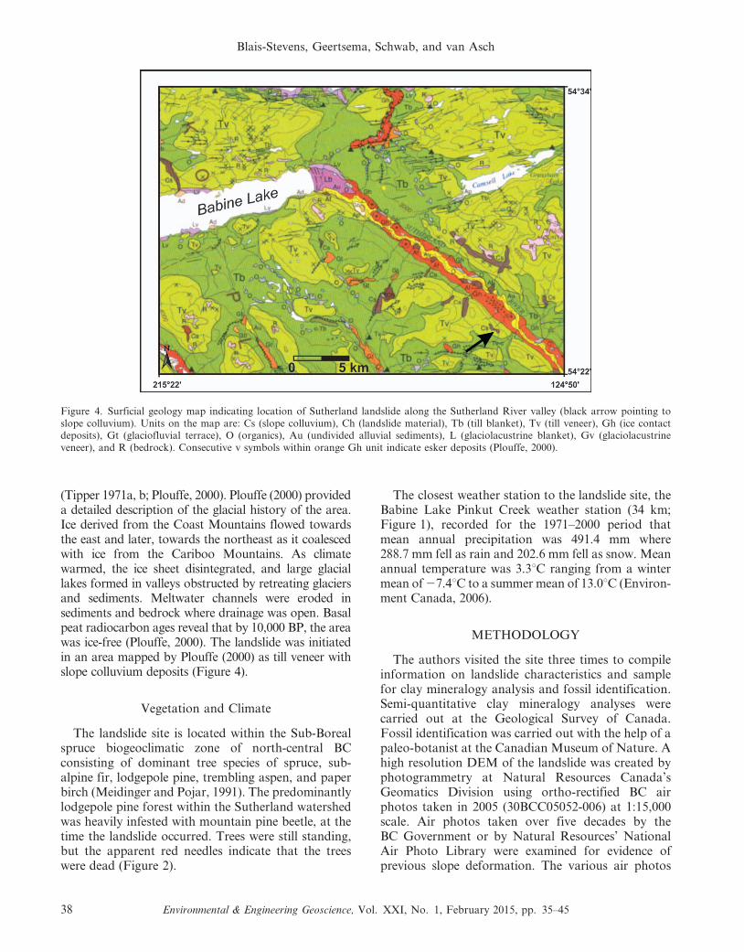
(Tipper 1971a, b; Plouffe, 2000). Plouffe (2000) provideda detailed description of the glacial history of the area.Ice derived from the Coast Mountains flowed towardsthe east and later, towards the northeast as it coalescedwith ice from the Cariboo Mountains. As climatewarmed, the ice sheet disintegrated, and large glaciallakes formed in valleys obstructed by retreating glaciersand sediments. Meltwater channels were eroded insediments and bedrock where drainage was open. Basalpeat radiocarbon ages reveal that by 10,000 BP, the areawas ice-free (Plouffe, 2000). The landslide was initiatedin an area mapped by Plouffe (2000) as till veneer withslope colluvium deposits (Figure 4).

Vegetation and Climate

The landslide site is located within the Sub-Borealspruce biogeoclimatic zone of north-central BCconsisting of dominant tree species of spruce, sub-alpine fir, lodgepole pine, trembling aspen, and paperbirch (Meidinger and Pojar, 1991). The predominantlylodgepole pine forest within the Sutherland watershedwas heavily infested with mountain pine beetle, at thetime the landslide occurred. Trees were still standing,but the apparent red needles indicate that the treeswere dead (Figure 2).

The closest weather station to the landslide site, theBabine Lake Pinkut Creek weather station (34 km;Figure 1), recorded for the 1971–2000 period thatmean annual precipitation was 491.4 mm where288.7 mm fell as rain and 202.6 mm fell as snow. Meanannual temperature was 3.3uC ranging from a wintermean of 27.4uC to a summer mean of 13.0uC (Environ-ment Canada, 2006).

METHODOLOGY

The authors visited the site three times to compileinformation on landslide characteristics and samplefor clay mineralogy analysis and fossil identification.Semi-quantitative clay mineralogy analyses werecarried out at the Geological Survey of Canada.Fossil identification was carried out with the help of apaleo-botanist at the Canadian Museum of Nature. Ahigh resolution DEM of the landslide was created byphotogrammetry at Natural Resources Canada’sGeomatics Division using ortho-rectified BC airphotos taken in 2005 (30BCC05052-006) at 1:15,000scale. Air photos taken over five decades by theBC Government or by Natural Resources’ NationalAir Photo Library were examined for evidence ofprevious slope deformation. The various air photos

Figure 4. Surficial geology map indicating location of Sutherland landslide along the Sutherland River valley (black arrow pointing toslope colluvium). Units on the map are: Cs (slope colluvium), Ch (landslide material), Tb (till blanket), Tv (till veneer), Gh (ice contactdeposits), Gt (glaciofluvial terrace), O (organics), Au (undivided alluvial sediments), L (glaciolacustrine blanket), Gv (glaciolacustrineveneer), and R (bedrock). Consecutive v symbols within orange Gh unit indicate esker deposits (Plouffe, 2000).



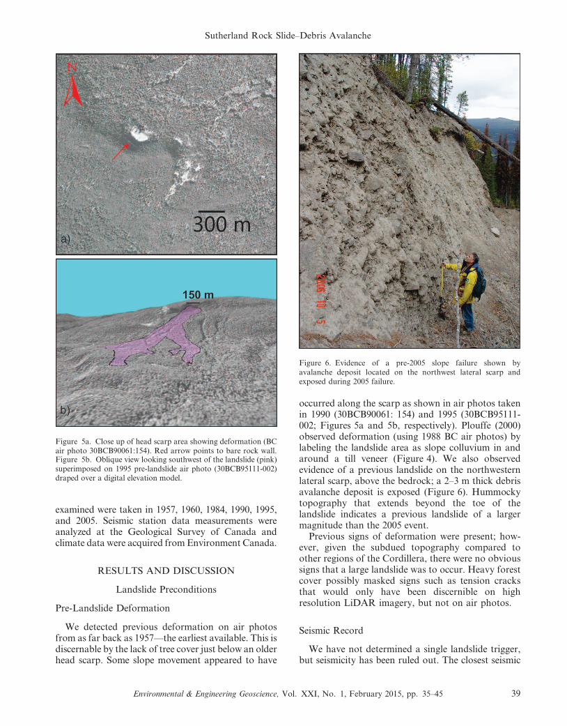
examined were taken in 1957, 1960, 1984, 1990, 1995,and 2005. Seismic station data measurements wereanalyzed at the Geological Survey of Canada andclimate data were acquired from Environment Canada.

RESULTS AND DISCUSSION

Landslide Preconditions

Pre-Landslide Deformation

We detected previous deformation on air photosfrom as far back as 1957—the earliest available. This isdiscernable by the lack of tree cover just below an olderhead scarp. Some slope movement appeared to have

occurred along the scarp as shown in air photos takenin 1990 (30BCB90061: 154) and 1995 (30BCB95111-002; Figures 5a and 5b, respectively). Plouffe (2000)observed deformation (using 1988 BC air photos) bylabeling the landslide area as slope colluvium in andaround a till veneer (Figure 4). We also observedevidence of a previous landslide on the northwesternlateral scarp, above the bedrock; a 2–3 m thick debrisavalanche deposit is exposed (Figure 6). Hummockytopography that extends beyond the toe of thelandslide indicates a previous landslide of a largermagnitude than the 2005 event.

Previous signs of deformation were present; how-ever, given the subdued topography compared toother regions of the Cordillera, there were no obvioussigns that a large landslide was to occur. Heavy forestcover possibly masked signs such as tension cracksthat would only have been discernible on highresolution LiDAR imagery, but not on air photos.

Seismic Record

We have not determined a single landslide trigger,but seismicity has been ruled out. The closest seismic

Figure 5a. Close up of head scarp area showing deformation (BCair photo 30BCB90061:154). Red arrow points to bare rock wall.Figure 5b. Oblique view looking southwest of the landslide (pink)superimposed on 1995 pre-landslide air photo (30BCB95111-002)draped over a digital elevation model.

Figure 6. Evidence of a pre-2005 slope failure shown byavalanche deposit located on the northwest lateral scarp andexposed during 2005 failure.



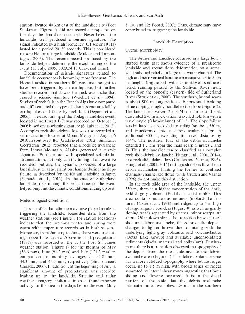
station, located 40 km east of the landslide site (FortSt. James; Figure 1), did not record earthquakes onthe day the landslide occurred. Nevertheless, thelandslide itself produced a seismic signature. Thesignal indicated by a high frequency (0.1 sec or 10 Hz)lasted for a period 20–30 seconds. This is consideredreasonable for a large landslide (Mulder and Lamon-tagne, 2005). The seismic record produced by thelandslide helped determine the exact timing of theevent (13 July, 2005, 0023:34:15 Universal Time).

Documentation of seismic signatures related tolandslide occurrences is becoming more frequent. TheHope landslide in southern BC was first thought tohave been triggered by an earthquake, but furtherstudies revealed that it was the rock avalanche thatcaused a seismic signature (Weichert et al., 1994).Studies of rock falls in the French Alps have comparedand differentiated the types of seismic signatures left byearthquakes and those by rock falls (Deparis et al.,2006). The exact timing of the Todagin landslide event,located in northwest BC, was recorded on October 3,2006 based on its seismic signature (Sakals et al., 2012).A complex rock slide-debris flow was also recorded atseismic stations located at Mount Meager on August 62010 in southwest BC (Guthrie et al., 2012). Similarly,Geertsema (2012) reported that a rock/ice avalanchefrom Lituya Mountain, Alaska, generated a seismicsignature. Furthermore, with specialized seismic in-strumentation, not only can the timing of an event berecorded, but also the dynamic processes of a largelandslide, such as acceleration changes during the slopefailure, as described for the Katani landslide in Japan(Yamada et al., 2013). In the case of Sutherlandlandslide, determining the exact time of the eventhelped pinpoint the climatic conditions leading up to it.

Meteorological Conditions

It is possible that climate may have played a role intriggering the landslide. Recorded data from theweather stations (see Figure 1 for station locations)indicate that the previous winter and spring werewarm with temperature records set in both seasons.Moreover, from January to June, there were oscillat-ing freeze thaw cycles. Above normal precipitation(177%) was recorded at the at the Fort St. Jamesweather station (Figure 1) for the months of May(56.6 mm), June (91.2 mm) and July (121.2 mm) incomparison to monthly averages of 31.8 mm,44.3 mm, and 46.5 mm, respectively (EnvironmentCanada, 2006). In addition, at the beginning of July, asignificant amount of precipitation was recordedleading up to the landslide. Satellite and radarweather imagery indicate intense thundershoweractivity for the area in the days before the event (July

8, 10, and 12; Foord, 2007). Thus, climate may havecontributed to triggering the landslide.

Landslide Description

Overall Morphology

The Sutherland landslide occurred in a large bowl-shaped basin that shows evidence of a prehistoriclandslide and recent slope deformation on a some-what subdued relief of a large meltwater channel. Thehigh and near-vertical head scarp measures up to 50 min height (Figure 3a) with a northwest-southeasttrend, running parallel to the Sullivan River fault,located on the opposite (eastern) side of SutherlandRiver (Struik et al., 2000). The southern, lateral scarpis about 900 m long with a sub-horizontal beddingplane dipping roughly parallel to the slope (Figure 2).The landslide involved 2.5–3 Mm3 of rock and soil,descended 270 m in elevation, travelled 1.45 km with atravel angle (fahrboschung) of 11u. The slope failurewas initiated as a rock slide traveling for about 550 m,and transformed into a debris avalanche for anadditional 900 m, extending its travel distance by164%. The northern fork of the debris avalancheextended 1.2 km from the main scarp (Figures 2 and7). Thus, the landslide can be classified as a complexrock slide-debris avalanche (Hungr et al., 2001, 2014),or a rock slide-debris flow (Cruden and Varnes, 1996).Hungr et al. (2001, 2014) distinguish debris flows fromdebris avalanches, limiting the former to confinedchannels (channelized flows) while Cruden and Varnes(1996) do not make this distinction.

In the rock slide area of the landslide, the upper550 m, there is a higher concentration of the dark,reddish-gray volcanic (Endako basalts) rubble. Thisarea contains numerous mounds (molard-like fea-tures; Cassie et al., 1988) and ridges up to 5 m highof large angular boulders (Figure 8) as well as gentlysloping treads separated by steeper, minor scarps. Atabout 550 m down slope, the transition between rockslide and debris avalanche, the color of the depositchanges to lighter brown due to mixing with theunderlying light gray volcanics and volcaniclastics(Ootsa Lake Group) and available unconsolidatedsediments (glacial material and colluvium). Further-more, there is a transition observed in topography ofthe deposit from the rock slide area to the debris-avalanche area (Figure 7). The debris avalanche zonehas a more subdued topography where lobate ridgesoccur, up to 1.5 m high, with broad zones of ridgesseparated by lateral shear zones suggesting that bothsliding and flowing occurred. It is in the distalportion of the slide that the debris avalanchebifurcated into two lobes. Debris in the southern



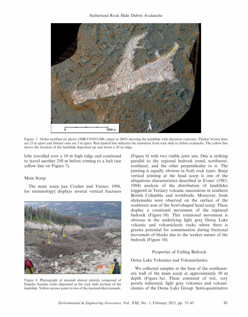
lobe travelled over a 10 m high ridge and continuedto travel another 250 m before coming to a halt (seeyellow line on Figure 7).

Main Scarp

The main scarp [see Cruden and Varnes, 1996,for terminology] displays several vertical fractures

(Figure 9) with two visible joint sets. One is strikingparallel to the regional bedrock trend, northwest-southeast, and the other perpendicular to it. Thejointing is equally obvious in both rock types. Steepvertical jointing at the head scarp is one of theubiquitous characteristics described in Evans’ (1983,1984) analysis of the distribution of landslidestriggered in Tertiary volcanic successions in southernBritish Columbia and worldwide. Moreover, freshslickensides were observed on the surface of thesouthwest arm of the bowl-shaped head scarp. Thesedisplay a rotational movement of the rupturedbedrock (Figure 10). This rotational movement isobvious in the underlying light gray Ootsa Lakevolcanic and volcaniclastic rocks where there isgreater potential for comminution during frictionalmovement of blocks due to the weaker nature of thebedrock (Figure 10).

Properties of Failing Bedrock

Ootsa Lake Volcanics and Volcaniclastics

We collected samples at the base of the southeast-ern wall of the main scarp at approximately 50 mdepth (Figure 3a). These consisted of wet, verypoorly indurated, light gray volcanics and volcani-clastics of the Ootsa Lake Group. Semi-quantitative

Figure 7. Ortho-rectified air photo (30BCC05052-006; taken in 2005) showing the landslide with elevation contours. Thicker brown linesare 25 m apart and thinner ones are 5 m apart. Red dashed line indicates the transition from rock slide to debris avalanche. The yellow lineshows the location of the landslide deposited up and down a 10 m ridge.

Figure 8. Photograph of mounds almost entirely composed ofEndako basaltic rocks deposited in the rock slide portion of thelandslide. Yellow arrows point to two of the (molard-like) mounds.



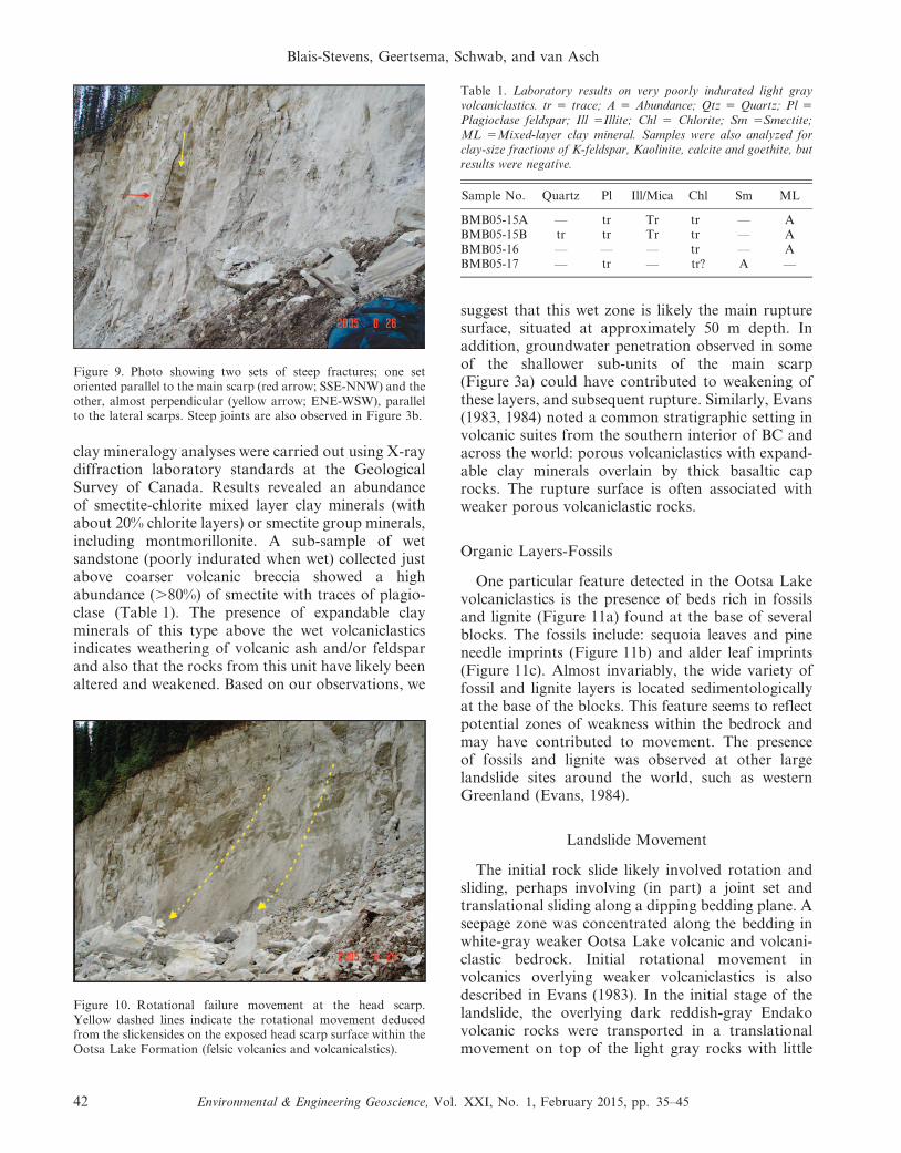
clay mineralogy analyses were carried out using X-raydiffraction laboratory standards at the GeologicalSurvey of Canada. Results revealed an abundanceof smectite-chlorite mixed layer clay minerals (withabout 20% chlorite layers) or smectite group minerals,including montmorillonite. A sub-sample of wetsandstone (poorly indurated when wet) collected justabove coarser volcanic breccia showed a highabundance (.80%) of smectite with traces of plagio-clase (Table 1). The presence of expandable clayminerals of this type above the wet volcaniclasticsindicates weathering of volcanic ash and/or feldsparand also that the rocks from this unit have likely beenaltered and weakened. Based on our observations, we

suggest that this wet zone is likely the main rupturesurface, situated at approximately 50 m depth. Inaddition, groundwater penetration observed in someof the shallower sub-units of the main scarp(Figure 3a) could have contributed to weakening ofthese layers, and subsequent rupture. Similarly, Evans(1983, 1984) noted a common stratigraphic setting involcanic suites from the southern interior of BC andacross the world: porous volcaniclastics with expand-able clay minerals overlain by thick basaltic caprocks. The rupture surface is often associated withweaker porous volcaniclastic rocks.

Organic Layers-Fossils

One particular feature detected in the Ootsa Lakevolcaniclastics is the presence of beds rich in fossilsand lignite (Figure 11a) found at the base of severalblocks. The fossils include: sequoia leaves and pineneedle imprints (Figure 11b) and alder leaf imprints(Figure 11c). Almost invariably, the wide variety offossil and lignite layers is located sedimentologicallyat the base of the blocks. This feature seems to reflectpotential zones of weakness within the bedrock andmay have contributed to movement. The presenceof fossils and lignite was observed at other largelandslide sites around the world, such as westernGreenland (Evans, 1984).

Landslide Movement

The initial rock slide likely involved rotation andsliding, perhaps involving (in part) a joint set andtranslational sliding along a dipping bedding plane. Aseepage zone was concentrated along the bedding inwhite-gray weaker Ootsa Lake volcanic and volcani-clastic bedrock. Initial rotational movement involcanics overlying weaker volcaniclastics is alsodescribed in Evans (1983). In the initial stage of thelandslide, the overlying dark reddish-gray Endakovolcanic rocks were transported in a translationalmovement on top of the light gray rocks with little

Figure 9. Photo showing two sets of steep fractures; one setoriented parallel to the main scarp (red arrow; SSE-NNW) and theother, almost perpendicular (yellow arrow; ENE-WSW), parallelto the lateral scarps. Steep joints are also observed in Figure 3b.

Figure 10. Rotational failure movement at the head scarp.Yellow dashed lines indicate the rotational movement deducedfrom the slickensides on the exposed head scarp surface within theOotsa Lake Formation (felsic volcanics and volcanicalstics).

Table 1. Laboratory results on very poorly indurated light grayvolcaniclastics. tr 5 trace; A 5 Abundance; Qtz 5 Quartz; Pl 5

Plagioclase feldspar; Ill 5Illite; Chl 5 Chlorite; Sm 5Smectite;ML 5Mixed-layer clay mineral. Samples were also analyzed forclay-size fractions of K-feldspar, Kaolinite, calcite and goethite, butresults were negative.

Sample No. Quartz Pl Ill/Mica Chl Sm ML

BMB05-15A — tr Tr tr — ABMB05-15B tr tr Tr tr — ABMB05-16 — — — tr — ABMB05-17 — tr — tr? A —



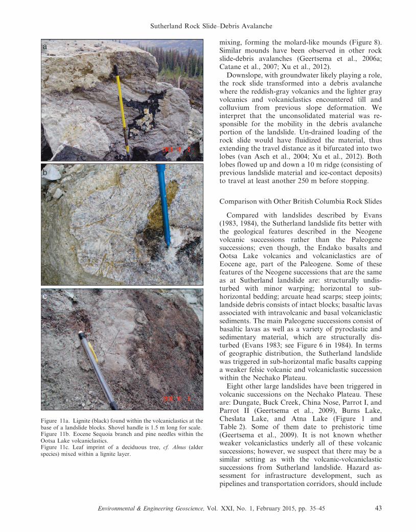
mixing, forming the molard-like mounds (Figure 8).Similar mounds have been observed in other rockslide-debris avalanches (Geertsema et al., 2006a;Catane et al., 2007; Xu et al., 2012).

Downslope, with groundwater likely playing a role,the rock slide transformed into a debris avalanchewhere the reddish-gray volcanics and the lighter grayvolcanics and volcaniclastics encountered till andcolluvium from previous slope deformation. Weinterpret that the unconsolidated material was re-sponsible for the mobility in the debris avalancheportion of the landslide. Un-drained loading of therock slide would have fluidized the material, thusextending the travel distance as it bifurcated into twolobes (van Asch et al., 2004; Xu et al., 2012). Bothlobes flowed up and down a 10 m ridge (consisting ofprevious landslide material and ice-contact deposits)to travel at least another 250 m before stopping.

Comparison with Other British Columbia Rock Slides

Compared with landslides described by Evans(1983, 1984), the Sutherland landslide fits better withthe geological features described in the Neogenevolcanic successions rather than the Paleogenesuccessions; even though, the Endako basalts andOotsa Lake volcanics and volcaniclastics are ofEocene age, part of the Paleogene. Some of thesefeatures of the Neogene successions that are the sameas at Sutherland landslide are: structurally undis-turbed with minor warping; horizontal to sub-horizontal bedding; arcuate head scarps; steep joints;landside debris consists of intact blocks; basaltic lavasassociated with intravolcanic and basal volcaniclasticsediments. The main Paleogene successions consist ofbasaltic lavas as well as a variety of pyroclastic andsedimentary material, which are structurally dis-turbed (Evans 1983; see Figure 6 in 1984). In termsof geographic distribution, the Sutherland landslidewas triggered in sub-horizontal mafic basalts cappinga weaker felsic volcanic and volcaniclastic successionwithin the Nechako Plateau.

Eight other large landslides have been triggered involcanic successions on the Nechako Plateau. Theseare: Dungate, Buck Creek, China Nose, Parrot I, andParrot II (Geertsema et al., 2009), Burns Lake,Cheslata Lake, and Atna Lake (Figure 1 andTable 2). Some of them date to prehistoric time(Geertsema et al., 2009). It is not known whetherweaker volcaniclastics underly all of these volcanicsuccessions; however, we suspect that there may be asimilar setting as with the volcanic-volcaniclasticsuccessions from Sutherland landslide. Hazard as-sessment for infrastructure development, such aspipelines and transportation corridors, should include

Figure 11a. Lignite (black) found within the volcaniclastics at thebase of a landslide blocks. Shovel handle is 1.5 m long for scale.Figure 11b. Eocene Sequoia branch and pine needles within theOotsa Lake volcaniclastics.Figure 11c. Leaf imprint of a deciduous tree, cf. Alnus (alderspecies) mixed within a lignite layer.



further detailed analyses of the Nechako Plateauvolcanics and underlying volcaniclastics. Some rec-ommendations include: detailed analyses of geotech-nical/geophysical properties of the materials, magni-tude/frequency of events, and spatial distributionusing high resolution imagery (e.g., LiDAR) relativeto the regional geology. Assessment of the volcanicand volcaniclastic successions is necessary to identifyand avoid potential landslide terrain that maycoincide with a transportation corridor across theNechako Plateau.

CONCLUSIONS

The Sutherland landslide is a complex rock slide-debris avalanche. It is located about 40 km west ofFort St. James, in Eocene volcanics and volcaniclas-tics of the Ootsa Lake Formation. The Sutherlandlandslide possesses a number of characteristics similarto large landslides triggered worldwide in Tertiarybasaltic successions. This includes thick horizontalcompetent basalts overlying weaker layered volcanicsand volcaniclastics and a very steep head scarpparallel to major faults and bedrock trend. Therapidly moving landslide involved 3 Mm3 of rock andsoil, travelled 1.45 km, and bifurcated in the runoutzone. The landslide area encompasses roughly 40 ha.The rupture surface is thought to be a very poorlyindurated volcaniclastic deposit of the Ootsa LakeGroup, rich in expandable clay minerals, and wet dueto abundant water seepage following above averageprecipitation. Initial landslide movement was rota-tional at the head scarp shown by presence ofrotational slickensides on white-gray volcanic andvolcaniclastic rocks in the southern lateral scarp.Historic air photos revealed that deformation wasongoing. Subdued topography and densely forestedterrain possibly masked signs that such a largecomplex landslide might occur. The exact time ofthe landslide was determined by a seismic signaturetypical of rock slides and avalanches. Above normalprecipitation in the months preceding the event mayhave been a contributing factor in triggering the

landslide. The prediction of these large rock ava-lanches and runout could be improved by detailedtopographic mapping. Bare earth LiDAR surveyswould have revealed the existence and extent of aprehistoric landslide, and possibly, precursor defor-mation features of the Sutherland landslide. Furtherstudies of past large landslides in volcanic successionswithin the Nechako Plateau could shed light on therole of weaker underlying volcaniclastics, as docu-mented in southern British Columbia and worldwide.

ACKNOWLEDGMENTS

The authors wish to thank A. Castagner fordrafting Figure 1, formatting text, and ortho-rectify-ing air photos. F. Salvopol provided the DEM fromthe post-landslide air photo. Clay mineralogy analy-ses were carried out by A. Grenier and J. Percival. T.Mulder and M. Lamontagne confirmed the exacttiming of the landslide occurrence from seismicrecords. V. Foord analyzed climate data. Fossils wereidentified by S. Cumbaa at the Museum of Nature.We wish to thank A. Plouffe at the Geological Surveyof Canada and two anonymous critical reviewersfor their invaluable comments and suggestions. Partof this research was funded by the Public SafetyGeoscience Program at Natural Resources Canada;GSC contribution number: 20130473.

REFERENCES

BARNES, E. M. AND ANDERSON, R. G., 1999, Bedrock geology ofthe Uncha Mountain area, northwestern Nechako River maparea, central British Columbia; in Current Research 1999-A,Geological Survey of Canada, pp. 129–138.

BLAIS-STEVENS, A.; GEERTSEMA, M.; SCHWAB, J. W.; VAN ASCH, T.;AND EGGINGTON, V. N., 2007, The 2005 Sutherland Riverrock slide-debris avalanche, central British Columbia. In 1st

International landslide conference, Vail Colorado AEG

Special Publication, No. 23, pp. 677–686.

CASSIE, J. W.; VAN GASSEN, W.; AND CRUDEN, D. M., 1988,Laboratory analogue of the formation of molards, cones ofrock avalanches: Geology, Vol. 16, pp. 735–738.

CATANE, S. G.; CABRIA, H. B.; TOMARONG, C. P., JR.; SATURAY,R. M., JR.; ZARCO, M. A. H.; AND PIOQUINTO, W. C., 2007,Catastrophic rockslide-debris avalanche at St. Bernard, South-ern Leyte, Philippines: Landslides, Vol. 4, No. 1, pp. 85–90.

CRUDEN, D. M. AND VARNES, D. J., 1996, Landslide types andprocesses: In: Turner, A. K. and Shuster, R. L. (Editors),Landslides: Investigation and Mitigation: TransportationResearch Board, Special Report 247, pp. 36–75.

DEPARIS, J. J.; JONGMANS, D.; COTTON, F.; AND THOUVENOT, F.,2006, Analysis of seismic records of rock falls in the FrenchAlps EGU General Assembly, Programs and abstracts,Vienna, Austria, 07894.

ENVIRONMENT CANADA, 2006, Climate Data, available at www.climate.weatheroffice.ec.gc.ca

EVANS, S. G., 1983, Landslides in layered volcanic successions with

particular reference to the tertiary rocks of south central

Table 2. Numbers refer to locations on Figure 1.

Number on map Landslide Name Coordinates

1 Buck Creek 54u229 N, 126u369 W2 Dungate 54u209 N, 126u349 W3 China Nose 54u239 N, 126u229 W4 Parrot I 54u059 N, 126u189 W5 Parrot II 54u049 N, 126u179 W6 Burns Lake 54u119 N, 125u399 W7 Cheslata Lake 53u439 N, 125u199 W8 Atna Lake 54u019 N, 127u429 W



British Columbia, Unpublished PhD Thesis, University ofAlberta, 350 p.

EVANS, S. G., 1984, Landslides in Tertiary basaltic successions:Proceedings for The IV International Symposium on landslides,Toronto 1: 503–510.

FOORD, V., 2007, personal communication, B.C. Ministry ofForests, Lands, and Natural Resources, Prince George,British Columbia.

GEERTSEMA, M., 2012, Initial Observations of the 11 June 2012Rock/Ice Avalanche, Lituya Mountain, Alaska: The First

Meeting of International Conssortium of Landslides Cold

Region Landslides Network, Harbin, China. 2012, pp. 49–54.

GEERTSEMA, M.; HUNGR, O.; SCHWAB, J. W.; AND EVANS, S. G.,2006, A large rock avalanche – debris flow at Pink Mountain,

northeastern British Columbia: Engineering Geology, Vol. 83,pp. 64–75.

GEERTSEMA, M.; SCHWAB, J. W.; BLAIS-STEVENS, A.; AND SAKALS, M.E., 2009, Landslides impacting linear infrastructure in westcentral British Columbia: Natural Hazards, Vol. 48, pp. 59–72.

GRAINGER, N. C. AND ANDERSON, R. G., 1999, Geology of theEocene Ootsa Lake Group in northern Nechako River andsouthern Fort Fraser map areas, central British Columbia; in

Current Research 1999-A; Geological Survey of Canada,

pp. 139–148.

GUTHRIE, R. H.; FRIELE, P.; ALLSTADT, K.; ROBERTS, N.; EVANS,

S. G.; DELANEY, K. B.; ROCHE, D.; CLAGUE, J. J.; AND JAKOB,M., 2012, The August 6 2010 Mount Meager rock slide-debris flow, Coast Mountians, British Columbia: character-istics, dynamics, and implications for hazard and riskassessment: Natural Hazards and Earth System Sciences,Vol. 12, pp. 1277–1294.

HASKIN, M.; SNYDER, L. D.; AND ANDERSON, R. G., 1998, TertiaryEndako Group volcanic and sedimentary rocks at four sites

in the Nechako River and Fort Fraser map areas, centralBritish Columbia; in Current Research 1998-A; GeologicalSurvey of Canada, pp. 155–164.

HOLLAND, S. S., 1976, Landforms of British Columbia: Aphysiographic outline: British Columbia Department ofMines and Petroleum Resources, Vol. 48, 138 p.

HUNGR, O.; EVANS, S. G.; BOVIS, M. J.; AND HUTCHINSON, J. N.,2001, A review of the classification of landslides of the flowtype: Environmental and Engineering Geoscience, Vol. VII,

pp. 221–238.

HUNGR, O.; LEROUIEIL, S.; AND PICARELLI, L., 2014, The Varnesclassification of landslide types, an update: Landslides, Vol.

11, pp. 167–194.

MASSEY, N. W. D.; MACINTYRE, D. G.; DESJARDINS, P. J.; AND

COONEY, R. T., 2005, Digital Geology Map of British

Columbia: Whole Province: B.C. Ministry of Energy andMines, GeoFile 2005-1.

MEIDINGER, D. AND POJAR, J., 1991, Ecosystems of BritishColumbia: British Columbia Ministry of Forests SpecialReport Series, Victoria BC, Vol. 6, 330 p.

MONGER, J. W. H.; SOUTHER, J. G.; AND GABRIELSE, H., 1972,Evolution of the Canadian Cordillera: a plate tectonic model:American Journal Science, Vol. 272, pp. 577–602.

MULDER, T. AND LAMONTAGNE, M., 2005, personal communica-tion, Geological Survey of Canada, Sidney, British Columbiaand Ottawa, Ontario.

PLOUFFE, A., 2000, Quaternary geology of the Fort Fraser andManson River map areas, central British Columbia: GeologicalSurvey Canada Bulletin, 554: 92 p.

SAKALS, M. E.; GEERTSEMA, M.; SCHWAB, J. W.; AND FOORD, V., 2012,The Todagin Creek landslide of October 3, 2006, NorthwestBritish Columbia, Canada: Landslides, Vol. 9, pp. 107–115.

STRUIK, L. C.; FALLAS, K.; HRUDEY, M. G.; AND WHALEN, J. B.,2000, Bedrock geology of the Burns Lake map area, BritishColumbia at scale 1:100,000: Geological Survey Canada,Open File 3840.

STRUIK, L. C. AND MACINTYRE, D. G., 2001, Introduction to thespecial issue of Canadian Journal of Earth Sciences: TheNechako NATMAP Project of the central Canadian Cordil-lera: Canadian Journal Earth Sciences, Vol. 38, pp. 486–493.

SUTHERLAND BROWN, A.; CATHRO, R. J.; PANTELEYEV, A.; AND NEY,C. S., 1970, Metallogeny of the Canadian Cordillera:Canadian Institute Mining Metallurgy Transactions, Vol. 74,pp. 121–145.

TIPPER, H. W., 1971a, Glacial geomorphology and Pleistocenehistory of central British Columbia: Geological Survey ofCanada Bulletin, Vol. 96, 89 p.

TIPPER, H. W., 1971b, Multiple glaciation in central British Columbia:Canadian Journal of Earth Sciences, Vol. 8, pp. 743–752.

VAN ASCH, T. W. J.; MALET, J.-P.; REMAITRE, A.; MAQUAIRE, O.,2004, Numerical modeling of the run-out of a muddy debrisflow. The effect of rheology on velocity and deposit thicknessalong the run-out track. In Lacerda, Ehrlich, Fontoura andSayao (Editors), Landslides: Evaluation and stabilization:Taylor and Francis Group, London, pp. 1433–1438.

WEICHERT, D.; HORNER, R. B.; AND EVANS, S. G., 1994, Seismicsignatures of landslides: the 1990 Brenda Mine collapse andthe 1965 Hope rockslides: Bulletin Seismic Society NorthAmerica, Vol. 84, No. 5, pp. 1523–1532.

YAMADA, M.; KUMAGAI, H.; MATSUSHI, Y.; AND MATSUZAWA, T.,2013, Dynamic landslide processes revealed by broadbandseismic records: Geophysical Research Letters, Vol. 40, pp. 2998–3002.

XU, Q.; SHANG, Y.; VAN ASCH, T. W. J.; WANG, S.; ZHANG, Z.; AND

DONG, X., 2012, Observations from the large, rapid Yigongrock slide-debris avalanche, southeast Tibet. CanadianGeotechnical Journal, Vol. 49, pp. 589–606, doi:10.1139/T2012-021



Modeling the Northern Coastline of Yucatan, Mexico,

with GENESIS

ROGER GONZALEZ-HERRERA1

Universidad Autonoma de Yucatan, Facultad de Ingenierıa, Av. Industrias nocontaminantes s/n, Periferico Norte, Merida, Yucatan, Mexico, CP 97000

ALFONSO SOLIS-PIMENTEL

Axis Ingenierıa S.A. de C.V., Consultants for Maritime and EnvironmentalEngineering, Merida, Yucatan, Mexico

CARLOS ZETINA-MOGUEL

Universidad Autonoma de Yucatan, Facultad de Ingenierıa, Av. Industrias nocontaminantes s/n, Periferico Norte, Merida, Yucatan, Mexico, CP 97000

ISMAEL MARINO-TAPIA

CINVESTAV–IPN, Unidad Merida, Km 6 Antigua Carretera a Progreso,Merida, Yucatan, Mexico, CP 97310

Key Terms: Coastal Erosion, GENESIS, Modeling,Simulation, Yucatan

ABSTRACT

The sandy coast of the State of Yucatan is subject tonatural and anthropogenic disturbances. Coastal ero-sion is a clear example of these disturbances. Manyactions have been proposed and implemented to combatthis problem; however, they have been counterproduc-tive. In the present work the evolution of the north-ern coastline of Yucatan, Mexico was studied. TheGENESIS model was applied to assess the effect ofgroins, breakwaters parallel to the coast and sandnourishment. The model was calibrated with availableoceanographic information; a thorough treatment ofthis information made the calibration consistent. It wasfound that: a) the obliquity of the incidence wave is themain cause of longitudinal sediment transport; b) thesediment transport produced as a result of the waveheight gradient along the coast is negligible; and c) theincident waves on the coast present very low energyand are governed mainly by local wind action. Theflexibility provided by the calibration coefficients inGENESIS allowed it to be used on the beaches ofYucatan; the values obtained during this researchreproduced in an acceptable manner both the morpho-logical changes observed and the volumetric variabilityof sediments. For these values and the calibration

conditions, the model can be applied to analyze theevolution of the beaches in the Yucatan. Furthermore, itreinforces the hypothesis that the groins have acceler-ated erosion, breakwaters off the coast are a viablealternative to coastal erosion in the study area, and theplacement of artificial sand is just a temporary solution.

INTRODUCTION

The study area corresponds to the coast of Yucatan(Figure 1). From a social and economic point of view,a large number of human activities of great impor-tance are carried out in this area (Yanez-Arancibia etal., 2013). The Yucatan Peninsula is a great platformand forms the northern part of the province of theGulf of Mexico’s coastal plain; it is made up oflimestone, dolomite, and evaporites. Sediments wereexposed to the surface between the Upper Cretaceousperiod and the Holocene epoch, with horizontallayers and carbonates gradually deposited, beingyounger toward the margins of the peninsula(Gondwe et al., 2010; Bauer-Gottwein et al., 2011).It is a geologically recent region formed by contribu-tions of unconsolidated sedimentary organic rockstructures. Underlying rock structures of higherconsolidation and older biogenic origin exist and aresubjected to lengthy processes of erosion andcementation. The unconsolidated material is presentas long barrier islands along the coast (Marino-Tapiaet al., 2007). These bars appear as broad, sandybeaches. They are primarily constituted of theremains of skeletal and calcareous structures or1Corresponding author email: [email protected].


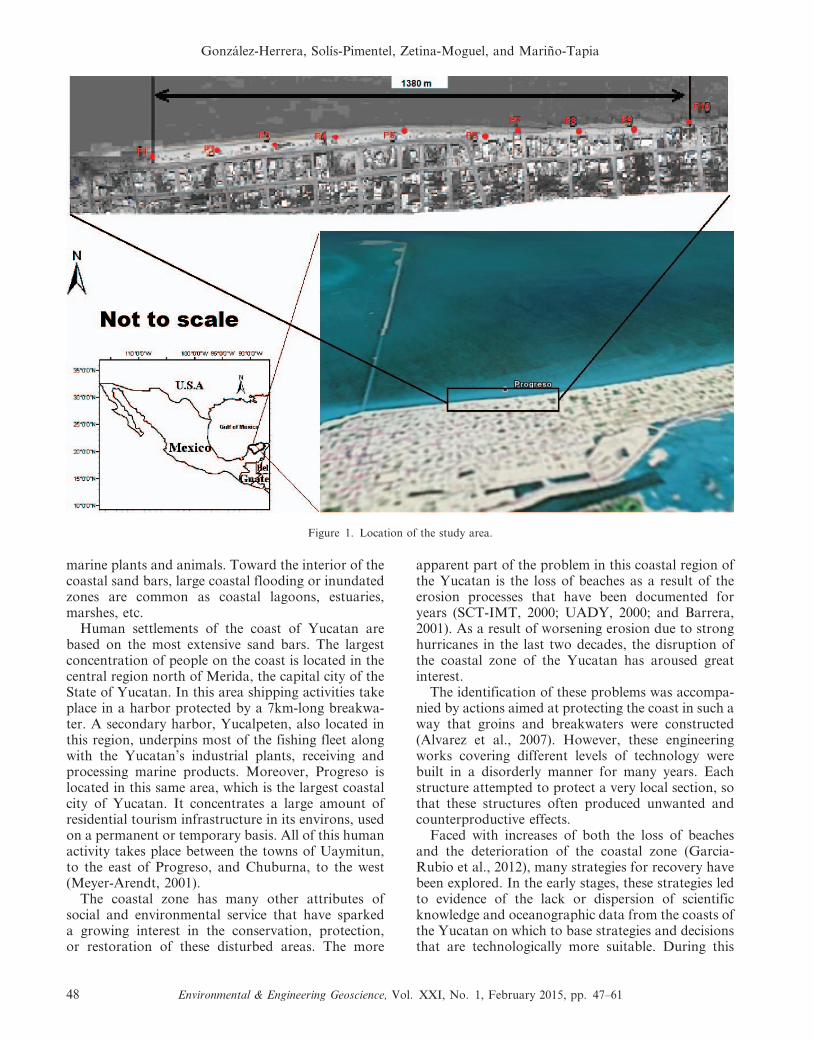
marine plants and animals. Toward the interior of thecoastal sand bars, large coastal flooding or inundatedzones are common as coastal lagoons, estuaries,marshes, etc.

Human settlements of the coast of Yucatan arebased on the most extensive sand bars. The largestconcentration of people on the coast is located in thecentral region north of Merida, the capital city of theState of Yucatan. In this area shipping activities takeplace in a harbor protected by a 7km-long breakwa-ter. A secondary harbor, Yucalpeten, also located inthis region, underpins most of the fishing fleet alongwith the Yucatan’s industrial plants, receiving andprocessing marine products. Moreover, Progreso islocated in this same area, which is the largest coastalcity of Yucatan. It concentrates a large amount ofresidential tourism infrastructure in its environs, usedon a permanent or temporary basis. All of this humanactivity takes place between the towns of Uaymitun,to the east of Progreso, and Chuburna, to the west(Meyer-Arendt, 2001).

The coastal zone has many other attributes ofsocial and environmental service that have sparkeda growing interest in the conservation, protection,or restoration of these disturbed areas. The more

apparent part of the problem in this coastal region ofthe Yucatan is the loss of beaches as a result of theerosion processes that have been documented foryears (SCT-IMT, 2000; UADY, 2000; and Barrera,2001). As a result of worsening erosion due to stronghurricanes in the last two decades, the disruption ofthe coastal zone of the Yucatan has aroused greatinterest.

The identification of these problems was accompa-nied by actions aimed at protecting the coast in such away that groins and breakwaters were constructed(Alvarez et al., 2007). However, these engineeringworks covering different levels of technology werebuilt in a disorderly manner for many years. Eachstructure attempted to protect a very local section, sothat these structures often produced unwanted andcounterproductive effects.

Faced with increases of both the loss of beachesand the deterioration of the coastal zone (Garcia-Rubio et al., 2012), many strategies for recovery havebeen explored. In the early stages, these strategies ledto evidence of the lack or dispersion of scientificknowledge and oceanographic data from the coasts ofthe Yucatan on which to base strategies and decisionsthat are technologically more suitable. During this

Figure 1. Location of the study area.

Gonzalez-Herrera, Solıs-Pimentel, Zetina-Moguel, and Marino-Tapia


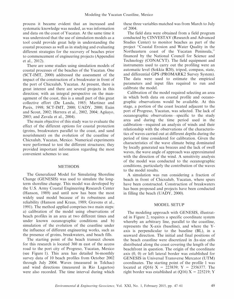
process it became evident that an increased andsystematic knowledge was needed, as was informationand data on the coast of Yucatan. At the same time itwas understood that the use of simulation models as atool could provide great help in understanding thecoastal processes as well as in studying and evaluatingdifferent strategies for the recovery of beaches priorto commencement of engineering projects (Appendiniet al., 2012).

There are some studies using simulation models ofcoastal processes of the beaches of the Yucatan. One(SCT-IMT, 2000) addressed the assessment of theimpact of the construction of a breakwater in front ofthe port of Chicxulub, Yucatan. At present, there isgreat interest and there are several projects in thisdirection; with an integral perspective on the man-agement of the coast, this is a small part of this greatcollective effort (De Landa, 1985; Martinez andPares, 1998; SCT-IMT, 2000; UADY, 2000; Euanand Scout, 2002; Herrera et al., 2002, 2004; Aguayo,2003; and Zavala et al., 2004).

The main objective of this study was to evaluate theeffect of the different options for coastal protection(groins, breakwaters parallel to the coast, and sandnourishment) on the evolution of the coastline ofChicxulub, Yucatan, Mexico. Numerical experimentswere performed to test the different structures; theyprovided important information regarding the mostconvenient schemes to use.

METHODS

The Generalized Model for Simulating ShorelineChange (GENESIS) was used to simulate the long-term shoreline change. This model was developed bythe U.S. Army Coastal Engineering Research Center(Hanson, 1989) and until now has been the mostwidely used model because of its robustness andreliability (Hanson and Kraus, 1989; Gravens et al.,1991). The method applied comprises two main steps:a) calibration of the model using observations ofbeach profiles in an area at two different times andunder known oceanographic conditions and b)simulation of the evolution of the coastline underthe influence of different engineering works, such asthe presence of groins, breakwaters, and beach fills.

The starting point of the beach transect chosenfor this research is located 360 m east of the accessroad to the port city of Progreso, Yucatan, Mexico(see Figure 1). This area has detailed bi-monthlysurvey data of 10 beach profiles from October 2002through July 2004. Waves (measured in Telchac)and wind directions (measured in Rio Lagartos)were also recorded. The time interval during which

these three variables matched was from March to Julyof 2004.

The field data were obtained from a field programconducted by CINVESTAV (Research and AdvancedStudies Center) to monitor beaches as part of theproject ‘‘Coastal Erosion and Water Quality in theNortheastern coast of the Yucatan Peninsula,’’financed by the National Council for Science andTechnology (CONACYT). The field equipment andinstruments used to carry out the profiling were anautomatic level (Sokkia B20), tripod, compass, state,and differential GPS (PROMARK2 Survey System).The data were used to estimate the empiricalparameters and input files required to run andcalibrate the model.

Calibration of the model required selecting an areain which both data on coastal profile and oceano-graphic observations would be available. At thisstage, a portion of the coast located adjacent to theport of Progreso, Yucatan, was selected. The lack ofoceanographic observations—specific to the studyarea and during the time period used in thecalibration—required an analysis of winds and theirrelationship with the observations of the characteris-tics of waves carried out at different depths during theperiod of time considered for calibration. Given thecharacteristics of the wave climate being dominatedby locally generated sea breezes and the lack of swellwaves, the wave angle of approach was approximatedwith the direction of the wind. A sensitivity analysisof the model was conducted to the oceanographicconditions, particularly the contribution of the wavesto the model results.

A simulation was run considering a fraction ofbeach in front of Chicxulub, Yucatan, where spurshave been constructed. Construction of breakwatershas been proposed and projects have been conductedin filling the beach (UADY, 2000).

MODEL SETUP

The modeling approach with GENESIS, illustrat-ed in Figure 2, requires a specific coordinate systemwhereby an arbitrary line, parallel to the coastline,represents the X-axis (baseline), and where the Y-axis is perpendicular to the baseline (BL), in aseaward direction. The initial and final positions ofthe beach coastline were discretized in Dx-size cellsdistributed along the coast covering the length of thebeachfront in question. The origin of the coordinateaxis (0, 0) or left lateral border was established forGENESIS in Universal Transverse Mercator (UTM)coordinates. The starting point of the profile 1 waslocated at (Q16) X 5 223839; Y 5 2356377. Theright border was established at (Q16) X 5 225219; Y

Modeling the Yucatan Coastline, Mexico


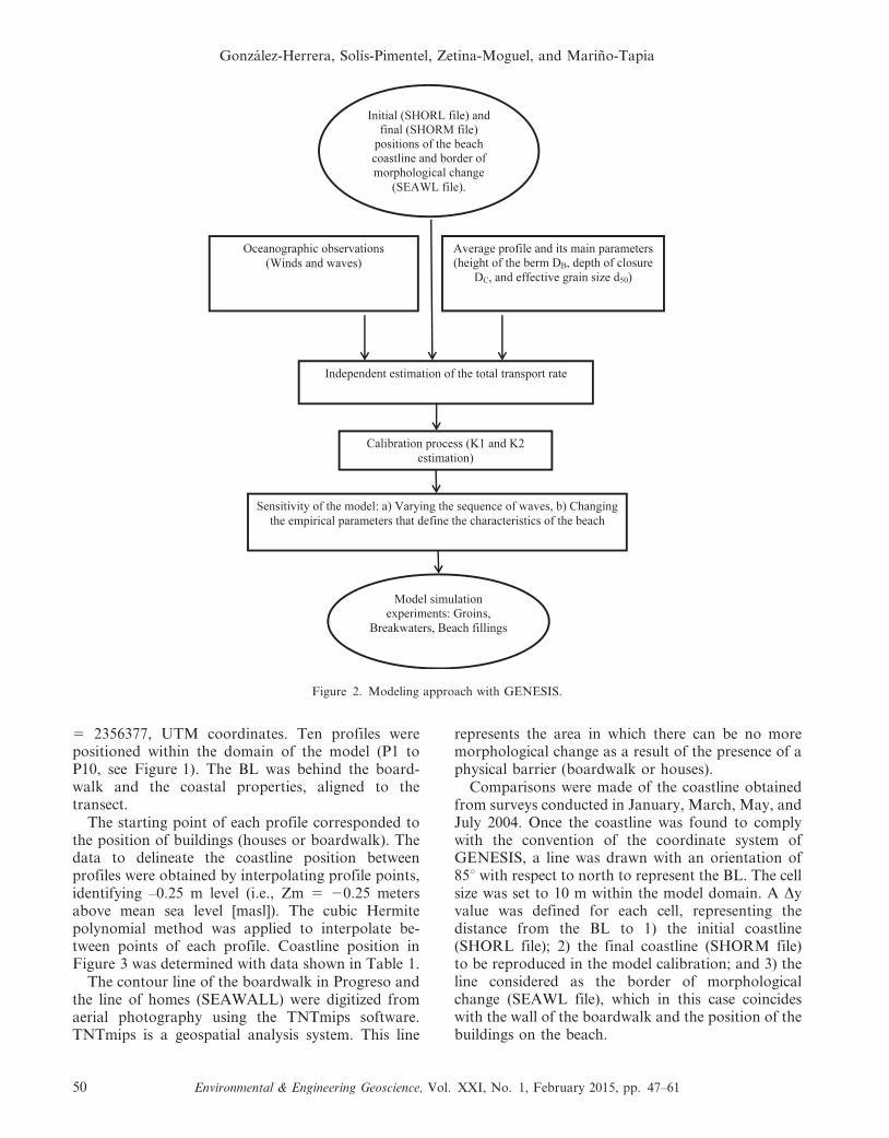
5 2356377, UTM coordinates. Ten profiles werepositioned within the domain of the model (P1 toP10, see Figure 1). The BL was behind the board-walk and the coastal properties, aligned to thetransect.

The starting point of each profile corresponded tothe position of buildings (houses or boardwalk). Thedata to delineate the coastline position betweenprofiles were obtained by interpolating profile points,identifying –0.25 m level (i.e., Zm 5 20.25 metersabove mean sea level [masl]). The cubic Hermitepolynomial method was applied to interpolate be-tween points of each profile. Coastline position inFigure 3 was determined with data shown in Table 1.

The contour line of the boardwalk in Progreso andthe line of homes (SEAWALL) were digitized fromaerial photography using the TNTmips software.TNTmips is a geospatial analysis system. This line

represents the area in which there can be no moremorphological change as a result of the presence of aphysical barrier (boardwalk or houses).

Comparisons were made of the coastline obtainedfrom surveys conducted in January, March, May, andJuly 2004. Once the coastline was found to complywith the convention of the coordinate system ofGENESIS, a line was drawn with an orientation of85u with respect to north to represent the BL. The cellsize was set to 10 m within the model domain. A Dyvalue was defined for each cell, representing thedistance from the BL to 1) the initial coastline(SHORL file); 2) the final coastline (SHORM file)to be reproduced in the model calibration; and 3) theline considered as the border of morphologicalchange (SEAWL file), which in this case coincideswith the wall of the boardwalk and the position of thebuildings on the beach.

Figure 2. Modeling approach with GENESIS.



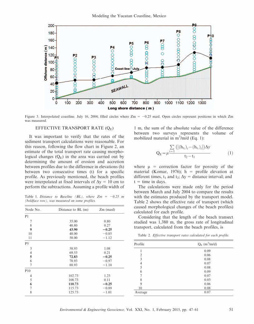
EFFECTIVE TRANSPORT RATE (QE)

It was important to verify that the rates of thesediment transport calculations were reasonable. Forthis reason, following the flow chart in Figure 2, anestimate of the total transport rate causing morpho-logical changes (QE) in the area was carried out bydetermining the amount of erosion and accretionbetween profiles due to the difference in elevations (h)between two consecutive times (t) for a specificprofile. As previously mentioned, the beach profileswere interpolated at fixed intervals of Dy 5 10 cm toperform the subtractions. Assuming a profile width of

1 m, the sum of the absolute value of the differencebetween two surveys represents the volume ofmobilized material in m3/m/d (Eq. 1):

QE~m

Pi~1

ht2ð Þi{ ht1

ð Þi��

Dy

t2{t1ð1Þ

where m 5 correction factor for porosity of thematerial (Komar, 1976); h 5 profile elevation atdifferent times, t1 and t2; Dy 5 distance interval; andt 5 time in days.

The calculations were made only for the periodbetween March and July 2004 to compare the resultswith the estimates produced by the transport model.Table 2 shows the effective rate of transport (whichcaused morphological changes of the beach profiles)calculated for each profile.

Considering that the length of the beach transectstudied was 1,380 m, the gross rate of longitudinaltransport, calculated from the beach profiles, is

Figure 3. Interpolated coastline. July 16, 2004; filled circles where Zm 5 20.25 masl. Open circles represent positions in which Zmwas measured.

Table 1. Distance to Baseline (BL), where Zm 5 20.25 m(boldface row), was measured on some profiles.

Node No. Distance to BL (m) Zm (masl)

P1

7 35.00 0.808 40.80 0.279 43.90 20.25

10 48.00 20.8511 58.00 21.12

P5

3 58.93 1.084 69.53 0.215 72.83 20.256 78.93 20.977 88.93 21.10

P10

4 102.73 1.235 108.73 0.116 110.73 20.257 115.73 20.898 125.73 21.01

Table 2. Effective transport rates calculated for each profile.

Profile QE (m3/m/d)

1 0.092 0.063 0.084 0.075 0.086 0.097 0.078 0.039 0.06

10 0.08Average 0.07



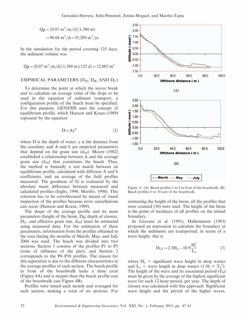
Qg~ 0:07 m3=m=d� �

1,380 mð Þ

~96:68 m3=d~35,289 m3=yr

In the simulation for the period covering 125 days,the sediment volume was

Qg~ 0:07 m3=m=d� �

1,380 mð Þ 125 dð Þ~12,085 m3

EMPIRICAL PARAMETERS (D50, DB, AND DC)

To determine the point at which the waves breakand to calculate an average value of the slope to beused in the equation of sediment transport, aconfiguration profile of the beach must be specified.For this purpose, GENESIS uses the concept ofequilibrium profile, which Hanson and Kraus (1989)represent by the equation

D~Ayb ð2Þ

where D is the depth of water; y is the distance fromthe coastline; and A and b are empirical parametersthat depend on the grain size (d50). Moore (1982)established a relationship between A and the averagegrain size (d50) that constitutes the beach. Thus,the method is basically a test match between anequilibrium profile, calculated with different A and bcoefficients, and an average of the field profilesmeasured. The goodness of fit is evaluated by theabsolute mean difference between measured andcalculated profiles (Inglis, 1996; Marino, 1998). Thiscriterion has to be corroborated by means of visualinspection of the profiles because error cancellationscan occur (Hanson and Kraus, 1989).

The shape of the average profile and its mainparameters (height of the berm, DB; depth of closure,DC; and effective grain size, d50) must be estimatedusing measured data. For the estimation of theseparameters, information from the profiles obtained inthe area during the months of March, May, and July2004 was used. The beach was divided into twosections. Section 1 consists of the profiles P1 to P5(zone of influence of the pier), and Section 2corresponds to the P6–P10 profiles. The reason forthis separation is due to the different characteristics inthe average profiles of each section. The beach profilein front of the boardwalk lacks a dune crest(Figure 4A) and is steeper than the beach profile eastof the boardwalk (see Figure 4B).

Profiles were tested each month and averaged foreach section, making a total of six sections. For

estimating the height of the berm, all the profiles thatwere counted (30) were used. The height of the bermis the point of incidence of all profiles on the inlandboundary.

In Gravens et al. (1991), Hallermeirer (1983)proposed an expression to calculate the boundary atwhich the sediments are transported; in terms of awave height, this is

DLT~2:3Ho{10:9H2

o

Loð3Þ

where Ho 5 significant wave height in deep watersand Lo 5 wave length in deep waters (1.56 3 TS

2).The height of the wave and its associated period (TS)must be given by the average of the highest significantwave for each 12-hour period, per year. The depth ofclosure was calculated with this approach. Significantwave height and the period of the higher waves,

Figure 4. (A). Beach profiles 1 to 5 in front of the boardwalk. (B).Beach profiles 6 to 10 east of the boardwalk.



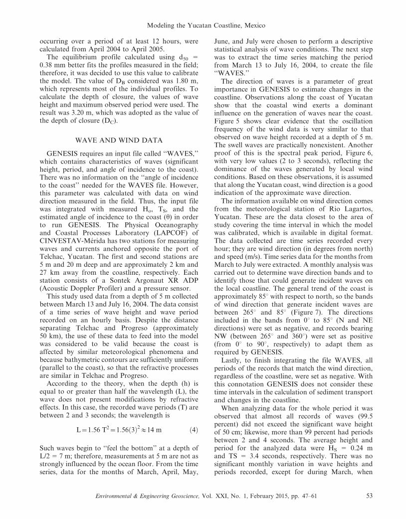
occurring over a period of at least 12 hours, werecalculated from April 2004 to April 2005.

The equilibrium profile calculated using d50 5

0.38 mm better fits the profiles measured in the field;therefore, it was decided to use this value to calibratethe model. The value of DB considered was 1.80 m,which represents most of the individual profiles. Tocalculate the depth of closure, the values of waveheight and maximum observed period were used. Theresult was 3.20 m, which was adopted as the value ofthe depth of closure (DC).

WAVE AND WIND DATA

GENESIS requires an input file called ‘‘WAVES,’’which contains characteristics of waves (significantheight, period, and angle of incidence to the coast).There was no information on the ‘‘angle of incidenceto the coast’’ needed for the WAVES file. However,this parameter was calculated with data on winddirection measured in the field. Thus, the input filewas integrated with measured Ho, TS, and theestimated angle of incidence to the coast (h) in orderto run GENESIS. The Physical Oceanographyand Coastal Processes Laboratory (LAPCOF) ofCINVESTAV-Merida has two stations for measuringwaves and currents anchored opposite the port ofTelchac, Yucatan. The first and second stations are5 m and 20 m deep and are approximately 2 km and27 km away from the coastline, respectively. Eachstation consists of a Sontek Argonaut XR ADP(Acoustic Doppler Profiler) and a pressure sensor.

This study used data from a depth of 5 m collectedbetween March 13 and July 16, 2004. The data consistof a time series of wave height and wave periodrecorded on an hourly basis. Despite the distanceseparating Telchac and Progreso (approximately50 km), the use of these data to feed into the modelwas considered to be valid because the coast isaffected by similar meteorological phenomena andbecause bathymetric contours are sufficiently uniform(parallel to the coast), so that the refractive processesare similar in Telchac and Progreso.

According to the theory, when the depth (h) isequal to or greater than half the wavelength (L), thewave does not present modifications by refractiveeffects. In this case, the recorded wave periods (T) arebetween 2 and 3 seconds; the wavelength is

L~1:56 T2~1:56 3ð Þ2&14 m ð4Þ

Such waves begin to ‘‘feel the bottom’’ at a depth ofL/2 5 7 m; therefore, measurements at 5 m are not asstrongly influenced by the ocean floor. From the timeseries, data for the months of March, April, May,

June, and July were chosen to perform a descriptivestatistical analysis of wave conditions. The next stepwas to extract the time series matching the periodfrom March 13 to July 16, 2004, to create the file‘‘WAVES.’’

The direction of waves is a parameter of greatimportance in GENESIS to estimate changes in thecoastline. Observations along the coast of Yucatanshow that the coastal wind exerts a dominantinfluence on the generation of waves near the coast.Figure 5 shows clear evidence that the oscillationfrequency of the wind data is very similar to thatobserved on wave height recorded at a depth of 5 m.The swell waves are practically nonexistent. Anotherproof of this is the spectral peak period, Figure 6,with very low values (2 to 3 seconds), reflecting thedominance of the waves generated by local windconditions. Based on these observations, it is assumedthat along the Yucatan coast, wind direction is a goodindication of the approximate wave direction.

The information available on wind direction comesfrom the meteorological station of Rio Lagartos,Yucatan. These are the data closest to the area ofstudy covering the time interval in which the modelwas calibrated, which is available in digital format.The data collected are time series recorded everyhour; they are wind direction (in degrees from north)and speed (m/s). Time series data for the months fromMarch to July were extracted. A monthly analysis wascarried out to determine wave direction bands and toidentify those that could generate incident waves onthe local coastline. The general trend of the coast isapproximately 85u with respect to north, so the bandsof wind direction that generate incident waves arebetween 265u and 85u (Figure 7). The directionsincluded in the bands from 0u to 85u (N and NEdirections) were set as negative, and records bearingNW (between 265u and 360u) were set as positive(from 0u to 90u, respectively) to adapt them asrequired by GENESIS.

Lastly, to finish integrating the file WAVES, allperiods of the records that match the wind direction,regardless of the coastline, were set as negative. Withthis connotation GENESIS does not consider thesetime intervals in the calculation of sediment transportand changes in the coastline.

When analyzing data for the whole period it wasobserved that almost all records of waves (99.5percent) did not exceed the significant wave heightof 50 cm; likewise, more than 99 percent had periodsbetween 2 and 4 seconds. The average height andperiod for the analyzed data were HS 5 0.24 mand TS 5 3.4 seconds, respectively. There was nosignificant monthly variation in wave heights andperiods recorded, except for during March, when



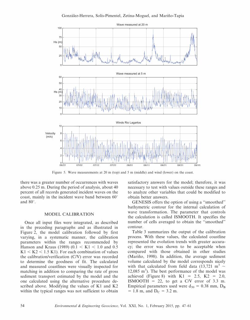
there was a greater number of occurrences with wavesabove 0.25 m. During the period of analysis, about 40percent of all records generated incident waves on thecoast, mainly in the incident wave band between 60uand 80u.

MODEL CALIBRATION

Once all input files were integrated, as describedin the preceding paragraphs and as illustrated inFigure 2, the model calibration followed by firstvarying, in a systematic manner, the calibrationparameters within the ranges recommended byHanson and Kraus (1989) (0.1 , K1 , 1.0 and 0.5K1 , K2 , 1.5 K1). For each combination of valuesthe calibration/verification (C/V) error was recordedto determine the goodness of fit. The calculatedand measured coastlines were visually inspected formatching in addition to comparing the rate of grosssediment transport estimated by the model and theone calculated using the alternative procedure de-scribed above. Modifying the values of K1 and K2within the typical ranges was not sufficient to obtain

satisfactory answers for the model; therefore, it wasnecessary to test with values outside these ranges andto analyze other variables that could be modified toobtain better answers.

GENESIS offers the option of using a ‘‘smoothed’’bathymetric contour for the internal calculation ofwave transformation. The parameter that controlsthe calculation is called ISMOOTH. It specifies thenumber of cells averaged to obtain the ‘‘smoothed’’contour.

Table 3 summarizes the output of the calibrationprocess. With these values, the calculated coastlinerepresented the evolution trends with greater accura-cy; the error was shown to be acceptable whencompared with those obtained in other studies(Marino, 1998). In addition, the average sedimentvolume calculated by the model corresponds nicelywith that calculated from field data (13,721 m3 ,12,085 m3). The best performance of the model wasachieved (Figure 8) with K1 5 2.5, K2 5 2.0,ISMOOTH 5 22, to get a C/V error of 3.3 m.Empirical parameters used were d50 5 0.38 mm, DB

5 1.8 m, and DC 5 3.2 m.

Figure 5. Wave measurements at 20 m (top) and 5 m (middle) and wind (lower) on the coast.



The sensitivity of the model was also tested toexamine the effect of some of the input variables onthe quality of the output data. These tests involve 1)varying the sequence of waves to investigate theirability to replicate acceptable changes in the coastlineand 2) changing the empirical parameters that definethe characteristics of the beach (d50, DB, and DC).

RESULTS

With the calibrated model, simulation experimentswere conducted to model the evolution of thecoastline in the presence of coastal protectionstructures (see Figure 2). This was carried out in a500-m transect located in the area of Chicxulub,Yucatan, approximately 5 km east of the area chosenfor the calibration of the model. For the simulationsthe initial coast line was set as reported in the studyarea by UADY (2000), corresponding to July 2000;its position and the SEAWALL line were obtainedfrom measurements by hand-drawing part of thestudy performed by UADY (2000) on a map (scale1:10,000).

The conditions under which the simulation exper-iments were run were 1) ‘‘normal’’ wave conditions(‘‘normal’’ conditions are those that do not occur innorthern and tropical storms, such as hurricanes); forthis reason the same data were used, time series ofwaves, with which the model was calibrated. 2) Timeintervals. The simulation time was the same in which

the model was calibrated; this is from March 13 toJuly 16, 2004 (125 days). 3) Size of the mesh. Thesame cell size (Dx 5 10 m), defined in the calibrationstage, was used; this was done to obtain a goodresolution in the positioning of the structures. 4)Values of empirical and calibration parameters.

The same empirical values obtained from field dataand the values of K1 and K2, with which the best resultswere obtained, as described in the model calibrationsection, were used. Therefore, the simulation experi-ments were run with the following values: K1 5 2.5, K25 2.0, and ISMOOTH 5 22. The simulation period was125 days, and the spatial intervals were 10-m incre-ments. For the conditions described above, the effects ofgroins, breakwaters off the coast, and beach fillingswere assessed. The specifications of the experimentsconducted are listed below.

Effect of Groins

Groins that existed in the area in July 2000 werelocated within the model domain. The position andlength of the groins were obtained from measure-ments by hand drawings using a map (scale 1:10,000)from the study performed by UADY (2000). It wasassumed that the water depth at the tip of thesubmerged groins is 0.5 m and that the permeability(ability of these structures to let sand pass throughthem) is 25 percent; it is also assumed that thesestructures are not completely waterproof because they

Figure 6. Monthly distribution of the wave period.



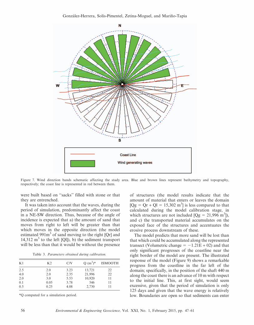
were built based on ‘‘sacks’’ filled with stone or thatthey are entrenched.

It was taken into account that the waves, during theperiod of simulation, predominantly affect the coastin a NE-SW direction. Thus, because of the angle ofincidence is expected that a) the amount of sand thatmoves from right to left will be greater than thatwhich moves in the opposite direction (the modelestimated 991m3 of sand moving to the right [Qr] and14,312 m3 to the left [Ql]), b) the sediment transportwill be less than that it would be without the presence

of structures (the model results indicate that theamount of material that enters or leaves the domain[Qg 5 Qr + Ql 5 15,302 m3] is less compared to thatcalculated during the model calibration stage, inwhich structures are not included [Qg 5 21,996 m3]),and c) the transported material accumulates on theexposed face of the structures and accentuates theerosive process downstream of these.

The model predicts that more sand will be lost thanthat which could be accumulated along the representedtransect (Volumetric change 5 21.21E + 02) and thatonly significant progresses of the coastline near theright border of the model are present. The illustratedresponse of the model (Figure 9) shows a remarkableprogress from the coastline in the far left of thedomain; specifically, in the position of the shaft 440 malong the coast there is an advance of 10 m with respectto the initial line. This, at first sight, would seemexcessive, given that the period of simulation is only125 days and given that the wave energy is relativelylow. Boundaries are open so that sediments can enter

Figure 7. Wind direction bands schematic affecting the study area. Blue and brown lines represent bathymetry and topography,respectively; the coast line is represented in red between them.

Table 3. Parameters obtained during calibration.

K1 K2 C/V Q (m3)* ISMOOTH

2.5 2.0 3.23 13,721 224.0 2.0 2.35 21,996 222.0 3.0 5.53 10,920 110.1 0.05 3.78 546 110.5 0.25 4.08 2,730 11

*Q computed for a simulation period.



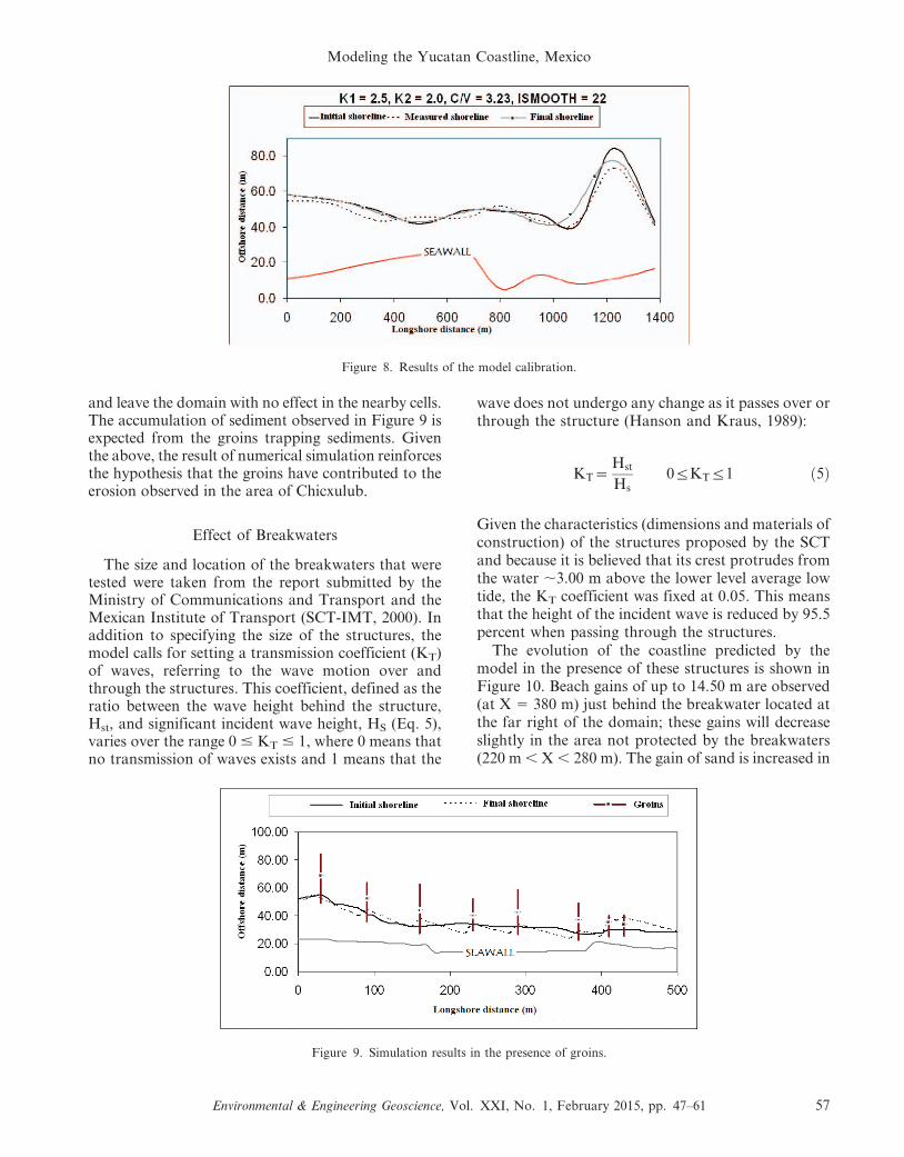
and leave the domain with no effect in the nearby cells.The accumulation of sediment observed in Figure 9 isexpected from the groins trapping sediments. Giventhe above, the result of numerical simulation reinforcesthe hypothesis that the groins have contributed to theerosion observed in the area of Chicxulub.

Effect of Breakwaters

The size and location of the breakwaters that weretested were taken from the report submitted by theMinistry of Communications and Transport and theMexican Institute of Transport (SCT-IMT, 2000). Inaddition to specifying the size of the structures, themodel calls for setting a transmission coefficient (KT)of waves, referring to the wave motion over andthrough the structures. This coefficient, defined as theratio between the wave height behind the structure,Hst, and significant incident wave height, HS (Eq. 5),varies over the range 0 # KT # 1, where 0 means thatno transmission of waves exists and 1 means that the

wave does not undergo any change as it passes over orthrough the structure (Hanson and Kraus, 1989):

KT~Hst

Hs0ƒKTƒ1 ð5Þ

Given the characteristics (dimensions and materials ofconstruction) of the structures proposed by the SCTand because it is believed that its crest protrudes fromthe water ,3.00 m above the lower level average lowtide, the KT coefficient was fixed at 0.05. This meansthat the height of the incident wave is reduced by 95.5percent when passing through the structures.

The evolution of the coastline predicted by themodel in the presence of these structures is shown inFigure 10. Beach gains of up to 14.50 m are observed(at X 5 380 m) just behind the breakwater located atthe far right of the domain; these gains will decreaseslightly in the area not protected by the breakwaters(220 m , X , 280 m). The gain of sand is increased in

Figure 8. Results of the model calibration.

Figure 9. Simulation results in the presence of groins.



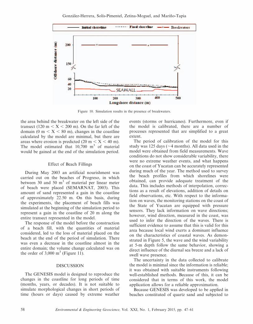
the area behind the breakwater on the left side of thetransect (120 m , X , 200 m). On the far left of thedomain (0 m , X , 80 m), changes in the coastlinecalculated by the model are minimal, but there areareas where erosion is predicted (20 m , X , 40 m).The model estimated that 10,700 m3 of materialwould be gained at the end of the simulation period.

Effect of Beach Fillings

During May 2003 an artificial nourishment wascarried out on the beaches of Progreso, in whichbetween 30 and 50 m3 of material per linear meterof beach were placed (SEMARNAT, 2003). Thisamount of sand represented a gain in the coastlineof approximately 22.50 m. On this basis, duringthe experiments, the placement of beach fills wassimulated at the beginning of the simulation period torepresent a gain in the coastline of 20 m along theentire transect represented in the model.

The response of the model before the constructionof a beach fill, with the quantities of materialconsidered, led to the loss of material placed on thebeach at the end of the period of simulation. Therewas even a decrease in the coastline almost in theentire domain; the volume change calculated was onthe order of 3,000 m3 (Figure 11).

DISCUSSION

The GENESIS model is designed to reproduce thechanges in the coastline for long periods of time(months, years, or decades). It is not suitable tosimulate morphological changes in short periods oftime (hours or days) caused by extreme weather

events (storms or hurricanes). Furthermore, even ifthe model is calibrated, there are a number ofprocesses represented that are simplified to a greatextent.

The period of calibration of the model for thisstudy was 125 days (,4 months). All data used in themodel were obtained from field measurements. Waveconditions do not show considerable variability, therewere no extreme weather events, and what happenson the coast of Yucatan can be accurately representedduring much of the year. The method used to surveythe beach profiles from which shorelines wereobtained, can provide adequate treatment of thedata. This includes methods of interpolation, correc-tions as a result of elevations, addition of details onfield observations, etc. With respect to the informa-tion on waves, the monitoring stations on the coast ofthe State of Yucatan are equipped with pressuresensors. They lack information on wave directions;however, wind direction, measured in the coast, wasused to infer the direction of the waves. There issufficient evidence to assume that this is valid for thisarea because local wind exerts a dominant influenceon the characteristics of coastal waves. As demon-strated in Figure 5, the wave and the wind variabilityat 5-m depth follow the same behavior, showing adirect influence of the diurnal sea breeze and a lack ofswell wave presence.

The uncertainty in the data collected to calibratethe model is minimal since the information is reliable;it was obtained with suitable instruments followingwell-established methods. Because of this, it can beconsidered that in terms of this work, the modelapplication allows for a reliable approximation.

Because GENESIS was developed to be applied inbeaches constituted of quartz sand and subjected to

Figure 10. Simulation results in the presence of breakwaters.



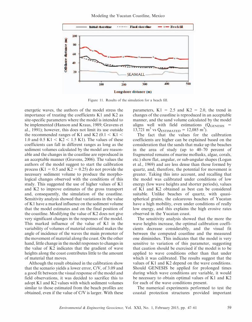
energetic waves, the authors of the model stress theimportance of treating the coefficients K1 and K2 assite-specific parameters where the model is intended tobe implemented (Hanson and Kraus, 1989; Gravens etal., 1991); however, this does not limit its use outsidethe recommended ranges of K1 and K2 (0.1 , K1 ,

1.0 and 0.5 K1 , K2 , 1.5 K1). The values of thesecoefficients can fall in different ranges as long as thesediment volumes calculated by the model are reason-able and the changes in the coastline are reproduced inan acceptable manner (Gravens, 2006). The values theauthors of the model suggest to start the calibrationprocess (K1 5 0.5 and K2 5 0.25) do not provide thenecessary sediment volume to produce the morpho-logical changes observed with the conditions of thisstudy. This suggested the use of higher values of K1and K2 to improve estimates of the gross transportand, consequently, the simulation of the coastline.Sensitivity analysis showed that variations in the valueof K1 have a marked influence on the sediment volumethat the model estimates and on the final position ofthe coastline. Modifying the value of K2 does not givevery significant changes in the responses of the model.This marked influence of the value of K1 in thevariability of volumes of material estimated makes theangle of incidence of the waves the main promoter ofthe movement of material along the coast. On the otherhand, little change in the model responses to changes inthe value of K2 indicates that the gradient of waveheights along the coast contributes little to the amountof material that moves.

Although the result obtained in the calibration showthat the scenario yields a lower error, C/V, of 3.09 anda good fit between the visual response of the model andfield observations, it was decided to sacrifice this toadopt K1 and K2 values with which sediment volumessimilar to those estimated from the beach profiles areobtained, even if the value of C/V is larger. With these

parameters, K1 5 2.5 and K2 5 2.0, the trend inchanges of the coastline is reproduced in an acceptablemanner, and the sand volume calculated by the modelaligns well with field estimations (QGENESIS 5

13,721 m3 vs QESTIMATED 5 12,085 m3).The fact that the values for the calibration

coefficients are higher can be explained based on theconsideration that the sands that make up the beachesin the area of study (up to 40–70 percent offragmented remains of marine mollusks, algae, corals,etc.) show flat, angular, or sub-angular shapes (Loganet al., 1969) and are less dense than those formed byquartz, and, therefore, the potential for movement isgreater. Taking this into account, and recalling thatthe model was calibrated under conditions of lowenergy (low wave heights and shorter periods), valuesof K1 and K2 obtained as best can be consideredsuitable. Unlike beaches of quartz, with quasi-spherical grains, the calcareous beaches of Yucatanhave a high mobility, even under conditions of reallylow energy, and this explains the high erosive ratesobserved in the Yucatan coast.

The sensitivity analysis showed that the more thewave heights increase, the optimal calibration coeffi-cients decrease considerably, and the visual fitbetween the computed coastline and the measuredone diminishes. This indicates that the model is verysensitive to variation of this parameter, suggestingthat caution should be exercised if the model is to beapplied to wave conditions other than that underwhich it was calibrated. The results suggest that thevalues of K1 and K2 depend on the wave conditions.Should GENESIS be applied for prolonged timesduring which wave conditions are variable, it wouldbe necessary to obtain optimal values of K1 and K2for each of the wave conditions present.

The numerical experiments performed to test thecoastal protection structures provided important

Figure 11. Results of the simulation for a beach fill.



information regarding the most convenient schemesto use. The simulation considering the presence ofgroins reproduces results in a manner that would beexpected of such schemes (i.e., accumulation of sandin the ‘‘updrift’’ structures, which reduces material tothe beaches ‘‘downdrift’’). This is corroborated bycomparing the response of the model with aerialphotographs of the area. Furthermore, the modelpredicts a net sediment loss in the whole domain,which is a clear indication that these structures cancontribute to the erosion process, as observed in thearea of Chicxulub and in many other regions of theYucatan coast.

On the other hand, model results considering thepresence of shore-parallel breakwaters off the coastshow that this geometry can help considerably theaccreting processes on local beaches. Sand accumu-lates in the protected part of the beach (behind thebreakwaters); this sand accumulation in the coastlinedecreases slightly in the fair space where the beach isnot directly protected by the structures, but the effectis very mild. Using the geometry of these structures,the model predicts that, in general, it will be a net gainof sediment on the beach. Despite the fact that suchstructures are a viable alternative to protect the coaststudied, this specific design could generate severalshortcomings due to its size, which include a hazardfor leisure navigation and the damaging of theaesthetic value of a tourist-oriented beach (byblocking of the view).

Finally, beach nourishment has been used world-wide as a successful beach protection scheme, which isespecially useful for sediment-starved beaches, such asthose of Yucatan. Nevertheless, this choice appearsless encouraging, as the model results suggest that itcould be lost rapidly (after just 4 months). Despitewhat recent beach profile analysis suggests—that thisrapid beach loss is overestimated—beach loss afternourishment is undeniable. Measures that could helpthe nourishment to remain longer could be increasingthe length of the beach fill or the volume of sand fed.Combination of beach protection schemes could alsobe a way to improve the performance of theseschemes.

CONCLUSIONS

The northern coast of the Yucatan peninsula hasbeen suffering the problem of shoreline retreat forseveral decades, and a series of beach protectionschemes have been implemented with limited degreesof success. A shoreline change model, GENESIS, wasimplemented on the beaches of the region, using a setof field data to define the shorelines, profile charac-teristics, and wave climate to study the effect on

shoreline stabilization of different beach protectionschemes, including groins (the most popular), offshoreparallel breakwaters, and beach nourishment.

Groins, as shown in practice and as evidence frommany regions of the world point out, are a veryinefficient scheme that generated sand accumulationonly for the first and second updrift structures, butthe overall result on the whole beach is widespreaderosion, with more sediment being lost than accumu-lated. Offshore breakwaters have the capability ofretaining sand, resulting in a beach width gain ofabout 5–10 m after a 4-month simulation. Neverthe-less, the geometry of the structures needs to becarefully planned so they do not represent a hazardfor navigation or an obstacle to the aesthetic value ofthe coast. Nowadays beach nourishment is one of thepreferred options for shore protection, as it re-nourishes sediment-starved beaches; however, for itto function properly it must be performed for enoughlengths along the coast and it must supply anadequate volume. For the region of interest, modelresults suggest that beach fills could be rapidly lost;therefore, a combination of appropriate beach fillsand shore parallel structures seem to offer anadequate beach protection scheme for this region.

ACKNOWLEDGMENTS

This study was carried out while the second authorwas granted a scholarship to carry out graduatestudies by the National Council of Science andTechnology (CONACYT); we are thankful for thesupport provided by FOMIX–CONACYT, throughthe projects ‘‘Coastal Erosion and Water Quality inthe Northeastern Coast of the Yucatan Peninsula’’and ‘‘Use Of Simulation Models for the Assessmentof Strategies for Physical Recovery of Beaches Basedon Coastal Engineering Works on the Coast ofYucatan’’; and the Center for Research and Ad-vanced Studies (CINVESTAV) in Merida, for pro-viding part of the field data used in this work. We arealso grateful with the personnel of the FIUADY andthe Physical Oceanography and Coastal ProcessesLaboratory (LAPCOF) at CINVESTAV, MeridaUnit, for the facilities granted for the developmentof this work.

REFERENCES

AGUAYO, G. M., 2003, Patrones de Variacion de la VegetacionAcuatica Sumergida en la Costa de Yucatan como Indicadoresde la Calidad del Agua Costera: Master’s Thesis, CINVES-TAV-IPN, Unidad Merida, Mexico.

ALVAREZ, E.; RUBIO, R.; AND RICALDE, H., 2007, Beach restorationwith geotextile tubes as submerged breakwaters in Yucatan,Mexico: Geotextiles Geomembranes, Vol. 25, pp. 233–241.



APPENDINI, C. M.; SALLES, P.; MENDOZA, E. T.; LOPEZ, J.; AND

TORRES-FREYERMUTH, A., 2012, Longshore sediment trans-port on the northern coast of the Yucatan Peninsula: JournalCoastal Research, Vol. 28, No. 6, pp. 1404–1417.

BARRERA, C. M., 2001, Deformacion en la Lınea de 1 Kilometrode Playa Comprendido Entre las Comisarıas de ChelemPuerto y Chuburna Puerto: Tesis de Licenciatura, Universi-dad Autonoma de Yucatan, Mexico.

BAUER-GOTTWEIN, P.; GONDWE, B. R. N.; CHARVET, G.; MARIN, L.E.; REBOLLEDO-VIEYRA, M.; AND MEREDIZ-ALONSO, G., 2011,Review: The Yucatan Peninsula karst aquifer, Mexico:Hydrogeology Journal, Vol. 19, pp. 507–524. doi:10.1007/s10040-010-0699-5

DE LANDA, D., 1985, Relacion de las Costas de Yucatan, Historia16: Cronicas de America 7. Madrid, Espana.

EUAN, A. J. AND SCOUT, W. G., 2002, Promoting integrated coastalmanagement in the Yucatan Peninsula, Mexico: JournalPolicy Studies, Vol. 12, pp. 1–16.

GARCIA-RUBIO, G.; HUNTLEY, D.; AND RUSSSELL, P., 2012,Assessing shoreline change using satellite-derived shorelinesin Progreso, Yucatan, Mexico, In Lynett, P. and Smith, J. M.(Editors), Coastal Engineering 2012, Proceedings of the 33rdCoastal Engineering. Santander, Spain. Published by theCoastal Engineering Research Council.

GONDWE, R. N.; LERER, S.; STINSEN, S.; MARIN, L.; REBOLLEDO-VIEYRA, M.; MEREDIZ-ALONSO, G.; AND BAUER-GOTTWEIN, P.,2010, Hydrogeology of the southeastern Yucatan Peninsula:New insights from water level measurements, geochemistry,geophysics and remote sensing: Journal Hydrology, Vol. 389,pp. 1–17. doi:10.1016/j.jhydrol.2010.04.044

GRAVENS, M. B.; KRAUS, N. C.; AND HANSON, H., 1991, GENESIS:Generalized Model for Simulating Shoreline Change. Report 2.Workbook and System User’s Manual: No. CERC-TR-89-19-2. U.S. Army Corps of Engineers. Coastal EngineeringResearch Center (CERC), Vicksburg, MS.

GRAVENS, M. B., 2006, personal communication.HALLERMEIER, R. J., 1983, Sand transport limits in coastal

structure design. In J. Richard Weggel (Editor). CoastalStructures ’83. Conference Proceedings. American Society ofCivil Engineers. New York, NY, pp. 703–716.

HANSON, H., 1989, GENESIS: A Generalized Shoreline ChangeNumerical Model: Journal Coastal Research, Vol. 5, No. 1,pp. 1–27.

HANSON, H. AND KRAUS, N. C., 1989, GENESIS: GeneralizedModel for Simulating Shoreline Change, Report 1. TechnicalReference: U.S. Army Corps of Engineers. Coastal Engineer-ing Research Center (CERC), Vicksburg, MS.

HERRERA, S. J. A.; COMIN, S. F.; AND CAPURRO, F. L., 2004, Losusos y abusos de la zona costera en la Penınsula de Yucatan.In El Manejo Costero en Mexico, Ed. EPOMEX, Mexico,pp. 387–396.

HERRERA, S. J. A.; MEDINA, G. N.; ZALDIVAR, J. A.; RAMIREZ, J.;AND TREJO, J., 2002, Trophic status in coastal waters ofthe Yucatan Peninsula (SE, Mexico) using water quality

indicators. In Brevibia, C. A. (Editor), EnvironmentalProblems in Coastal Regions IV: Wit-Press, pp. 351–359.

INGLIS, M. L., 1996, A Numerical Model Study Using GENESISV.3 of a Macrotidal, Shingle Beach after Construction ofExtensive Sea Defenses at Sidmouth, Devon: M.S. Thesis,University of Plymouth, U.K.

KOMAR, P. D., 1976, Beach Processes and Sedimentation: Prentice-Hall, Englewood Cliffs, NJ.

LOGAN, B. W.; HARDING, J. L.; AHR, W. M.; WILLIAMS, J. D.; AND

SNEAD, R. G., 1969, Carbonate Sediments and Reefs, YucatanShelf, Mexico: American Association of Petroleum Geolo-gists, Washington, DC.

MARINO, T. I., 1998, Morphological Changes on Teignmouth Beach,South Devon, UK: A Comparison between Field Observations andNumerical Model: M.S. Thesis, University of Plymouth, U.K.

MARINO-TAPIA, I.; RUSSELL, P. E.; O’HARE, T. J.; DAVIDSON,M. A.; AND HUNTLEY, D. A., 2007, Cross-shore sedimenttransport on natural beaches and their relation to sand barmigration patterns: Part 1. Field observations: JournalGeophysical Research, Vol. 112, p. C03001. doi:10.1029/2005JC002893

MARTINEZ, L. B. AND PARES, S., 1998, Circulacion del Golfo deMexico Inducida por Mareas, Viento y Corrientes deYucatan: Ciencias Marinas, Vol. 24, No. 1, pp. 65–93.

MEYER-ARENDT, K. J., 2001, Recreational development andshoreline modification along the north coast of Yucatan,Mexico. Tourism Geographies: International Journal TourismSpace, Place Environment, Vol. 3, No. 1, pp. 87–104. doi:10.1080/14616680010008720

MOORE, B., 1982, Beach Profile Evolution in Response to Changesin Water Level and Wave Height: M.S. Thesis, Department ofCivil Engineering, University of Delaware, Newark, DE.

SCT-IMT, 2000, Reporte Tecnico Preliminar del Estudio deDinamica Costera Para Definir las Obras de Proteccion Contrala Erosion de la Playa Localizada entre Huaymitun y Chuburna,Yuc: Secretarıa de Comunicaciones y Transportes–InstitutoMexicano del Transporte, Mexico.

SEMARNAT, 2003, Erosion Costera, Secretarıa de MedioAmbiente y Recursos Naturales, Mexico: Electronic docu-ment, available at www.semarnat.gob.mx/yucatan/ErosionCostera/ProgramaRecuperacion03.shtm

UADY, 2000, Modelo Hidrodinamico del Arrastre de Arenas ySedimentos en Chicxulub Puerto, Estado de Yucatan: Uni-versidad Autonoma de Yucatan, Mexico.

YANEZ-ARANCIBIA, A.; DAY, J. W.; AND REYES, E., 2013, Under-standing the coastal ecosystem-based management approach inthe Gulf of Mexico. In Brock, J. C.; Barras, J. A.; and Williams,S. J. (Editors), Understanding and predicting change in thecoastal ecosystems of the Northern Gulf of Mexico: JournalCoastal Research, Vol. 63, Special Issue, pp. 243–261.

ZAVALA, H. J.; GALLEGOS, A.; MOREY, S. L.; AND O’BRIEN, J. J.,2004, Upwelling and circulation on the Western Shelf Gulfof Mexico. In XII International Conference on Physics ofEstuarine and Coastal Seas: Merida, Mexico.



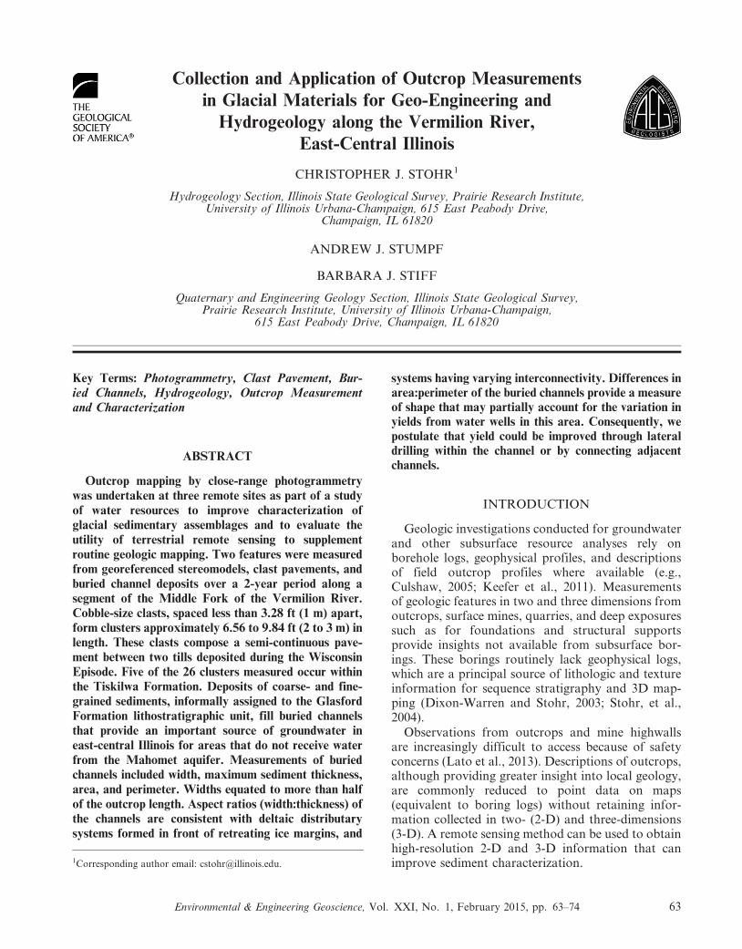
Collection and Application of Outcrop Measurements

in Glacial Materials for Geo-Engineering and

Hydrogeology along the Vermilion River,

East-Central Illinois

CHRISTOPHER J. STOHR1

Hydrogeology Section, Illinois State Geological Survey, Prairie Research Institute,University of Illinois Urbana-Champaign, 615 East Peabody Drive,

Champaign, IL 61820

ANDREW J. STUMPF

BARBARA J. STIFF

Quaternary and Engineering Geology Section, Illinois State Geological Survey,Prairie Research Institute, University of Illinois Urbana-Champaign,

615 East Peabody Drive, Champaign, IL 61820

Key Terms: Photogrammetry, Clast Pavement, Bur-ied Channels, Hydrogeology, Outcrop Measurementand Characterization

ABSTRACT

Outcrop mapping by close-range photogrammetrywas undertaken at three remote sites as part of a studyof water resources to improve characterization ofglacial sedimentary assemblages and to evaluate theutility of terrestrial remote sensing to supplementroutine geologic mapping. Two features were measuredfrom georeferenced stereomodels, clast pavements, andburied channel deposits over a 2-year period along asegment of the Middle Fork of the Vermilion River.Cobble-size clasts, spaced less than 3.28 ft (1 m) apart,form clusters approximately 6.56 to 9.84 ft (2 to 3 m) inlength. These clasts compose a semi-continuous pave-ment between two tills deposited during the WisconsinEpisode. Five of the 26 clusters measured occur withinthe Tiskilwa Formation. Deposits of coarse- and fine-grained sediments, informally assigned to the GlasfordFormation lithostratigraphic unit, fill buried channelsthat provide an important source of groundwater ineast-central Illinois for areas that do not receive waterfrom the Mahomet aquifer. Measurements of buriedchannels included width, maximum sediment thickness,area, and perimeter. Widths equated to more than halfof the outcrop length. Aspect ratios (width:thickness) ofthe channels are consistent with deltaic distributarysystems formed in front of retreating ice margins, and

systems having varying interconnectivity. Differences inarea:perimeter of the buried channels provide a measureof shape that may partially account for the variation inyields from water wells in this area. Consequently, wepostulate that yield could be improved through lateraldrilling within the channel or by connecting adjacentchannels.

INTRODUCTION

Geologic investigations conducted for groundwaterand other subsurface resource analyses rely onborehole logs, geophysical profiles, and descriptionsof field outcrop profiles where available (e.g.,Culshaw, 2005; Keefer et al., 2011). Measurementsof geologic features in two and three dimensions fromoutcrops, surface mines, quarries, and deep exposuressuch as for foundations and structural supportsprovide insights not available from subsurface bor-ings. These borings routinely lack geophysical logs,which are a principal source of lithologic and textureinformation for sequence stratigraphy and 3D map-ping (Dixon-Warren and Stohr, 2003; Stohr, et al.,2004).

Observations from outcrops and mine highwallsare increasingly difficult to access because of safetyconcerns (Lato et al., 2013). Descriptions of outcrops,although providing greater insight into local geology,are commonly reduced to point data on maps(equivalent to boring logs) without retaining infor-mation collected in two- (2-D) and three-dimensions(3-D). A remote sensing method can be used to obtainhigh-resolution 2-D and 3-D information that canimprove sediment characterization.1Corresponding author email: [email protected].


Remote measuring by terrestrial or close-rangephotogrammetry using uncalibrated cameras is awell-established, low-cost method of collecting fielddata (Karara, 1972; Karara and Abdel-Aziz, 1974).The delineation of features by close-range photo-grammetric techniques is analogous to the use ofvertical stereomodels for geologic mapping withprojection stereoplotters (Rabben et al., 1960; Moffittand Mikhail, 1980; Avery and Berlin, 1985).

Remote sensing techniques, such as photography,surveying, close-range photogrammetry, and laserscanning, offer important opportunities to supple-ment traditional geologic mapping methods bycreating a georeferenced 3-D gridded model uponwhich sedimentary features on an exposed surface canbe delineated and measured (Xu et al., 2000; Bellianet al., 2005; Haneberg, 2008; Stohr et al., 2011).Furthermore, with image processing and field obser-vations, additional information or consultation notobtained at the site can be measured in a virtualrevisit. These relatively new techniques requiresophisticated instruments, software, and expertisenot in common geologic practice. Only a feweducational institutions teach these methods as partof their field mapping courses (Whitmeyer et al.,2009). Consequently, integration of these methodsinto the geosciences curriculum has been slow.

For this study, two sedimentary features weremeasured twice at three sites, namely, clast (cobbleand boulder) pavements and channel deposits. Theformer are of interest because of potential damage toexcavating equipment and interference in drilling anddriving sheet piles (Sauer, 1974). The Illinois StateGeological Survey has received inquiries about thecharacter of boulder pavements from consultantsperforming excavations in the Midwestern states.This study provides the measurements about thecontinuity of the glacial sedimentary feature.

The principal features of interest are buriedmeltwater channels that are now exposed in glacialsediments interpreted to have been deposited duringthe deglacial phase of the Illinois Episode glaciation.These channels are filled by coarse-grained sedimentthat constitutes a local aquifer, and are recognized asan important source of groundwater (Kempton et al.,1981), especially in areas not receiving water from theMahomet aquifer. Because water wells completed inthis aquifer (formed during the Illinois Episode) havelow to moderate pumpage rates, information con-cerning the distribution, character, and dimensions ofthese buried channels will assist water specialists byimproving the maps and models used to developwater management strategies. Improvement of yieldsfrom wells can reduce problems during drought and

allow rural residents and farmers to expand commer-cial and personal use of water resources.

GEOLOGY

Outcrops analyzed in this study were selected froma 2-mi (3-km) reach of river length of the MiddleFork of the Vermilion River, a National ScenicRiver that includes a State Fish and Wildlife Area(Figure 1). The outcrops were accessed from threesites, Blue Hole, Higginsville, and Porter Cemetery,informally named for nearby geographic locations orlocal cultural features. The outcrop at the Blue Holesite is situated along a bank at a right-angle bend inthe river. The Higginsville outcrop is located a shortdistance downstream of the Blue Hole site along anorth-to-south linear bank of the river. The outcropat the Porter Cemetery site is situated at a bend in theriver oriented N32uW. The sites were chosen becauseof their accessibility, the variety of sediments exposed,and the extent of the exposures (Table 1).

The three sites are located in a river valley that isincised into subglacial and proglacial deposits ofmultiple glaciations. The sediments exposed inoutcrops at these sites are assigned to two separateglacial events. Deposits of the more recent WisconsinEpisode include the Yorkville Member till andBatestown Member till of the Lemont Formation,and the Tiskilwa Formation till. Underlying these aredeposits of the Illinois Episode, including sediment ofthe upper and lower units of the Vandalia Member ofthe Glasford Formation (Figure 2).

Inset into this diamicton are glacial meltwaterchannels of the upper unit of the Vandalia Member ofthe Glasford Formation filled with deposits consistingof horizontally bedded to cross-bedded sand andgravel, or laminated to bedded silt and clay. In someplaces, the channels are cut deeper and extend into theunderlying till of the lower unit of the VandaliaMember of the Glasford Formation.

Detailed investigation of these outcrops revealed anotable clast pavement between tills of the BatestownMember and Tiskilwa Formation (Figures 3, 4, and5). Although these tills have very similar textures, theunits can be easily distinguished by their distinctivecolor and surface weathering. In some places, thecontact between them has been obscured by materialthat has fallen on the slope from above.

Clast pavements were delineated at three sites;however, only the pavement at the Higginsville sitewas entirely accessible. In earlier studies undertakenat the Higginsville site, Voorhees (1996, 1998)excavated and described a clast pavement ‘‘cobblezone’’ in considerable detail. The exact location of thepit and outcrop studied by Voorhees is not known but

Stohr, Stumpf, and Stiff


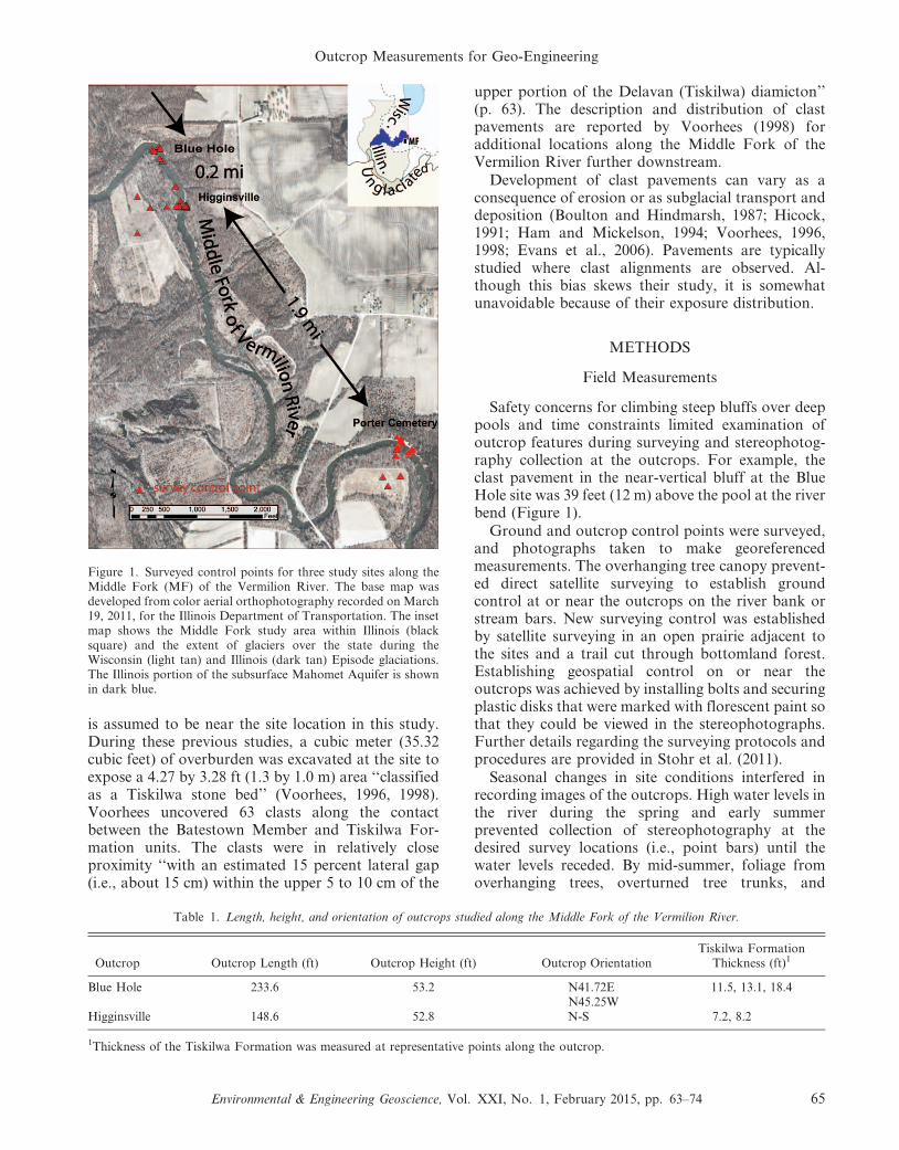
is assumed to be near the site location in this study.During these previous studies, a cubic meter (35.32cubic feet) of overburden was excavated at the site toexpose a 4.27 by 3.28 ft (1.3 by 1.0 m) area ‘‘classifiedas a Tiskilwa stone bed’’ (Voorhees, 1996, 1998).Voorhees uncovered 63 clasts along the contactbetween the Batestown Member and Tiskilwa For-mation units. The clasts were in relatively closeproximity ‘‘with an estimated 15 percent lateral gap(i.e., about 15 cm) within the upper 5 to 10 cm of the

upper portion of the Delavan (Tiskilwa) diamicton’’(p. 63). The description and distribution of clastpavements are reported by Voorhees (1998) foradditional locations along the Middle Fork of theVermilion River further downstream.

Development of clast pavements can vary as aconsequence of erosion or as subglacial transport anddeposition (Boulton and Hindmarsh, 1987; Hicock,1991; Ham and Mickelson, 1994; Voorhees, 1996,1998; Evans et al., 2006). Pavements are typicallystudied where clast alignments are observed. Al-though this bias skews their study, it is somewhatunavoidable because of their exposure distribution.

METHODS

Field Measurements

Safety concerns for climbing steep bluffs over deeppools and time constraints limited examination ofoutcrop features during surveying and stereophotog-raphy collection at the outcrops. For example, theclast pavement in the near-vertical bluff at the BlueHole site was 39 feet (12 m) above the pool at the riverbend (Figure 1).

Ground and outcrop control points were surveyed,and photographs taken to make georeferencedmeasurements. The overhanging tree canopy prevent-ed direct satellite surveying to establish groundcontrol at or near the outcrops on the river bank orstream bars. New surveying control was establishedby satellite surveying in an open prairie adjacent tothe sites and a trail cut through bottomland forest.Establishing geospatial control on or near theoutcrops was achieved by installing bolts and securingplastic disks that were marked with florescent paint sothat they could be viewed in the stereophotographs.Further details regarding the surveying protocols andprocedures are provided in Stohr et al. (2011).

Seasonal changes in site conditions interfered inrecording images of the outcrops. High water levels inthe river during the spring and early summerprevented collection of stereophotography at thedesired survey locations (i.e., point bars) until thewater levels receded. By mid-summer, foliage fromoverhanging trees, overturned tree trunks, and

Figure 1. Surveyed control points for three study sites along theMiddle Fork (MF) of the Vermilion River. The base map wasdeveloped from color aerial orthophotography recorded on March19, 2011, for the Illinois Department of Transportation. The insetmap shows the Middle Fork study area within Illinois (blacksquare) and the extent of glaciers over the state during theWisconsin (light tan) and Illinois (dark tan) Episode glaciations.The Illinois portion of the subsurface Mahomet Aquifer is shownin dark blue.

Table 1. Length, height, and orientation of outcrops studied along the Middle Fork of the Vermilion River.

Outcrop Outcrop Length (ft) Outcrop Height (ft) Outcrop OrientationTiskilwa Formation

Thickness (ft)1

Blue Hole 233.6 53.2 N41.72E 11.5, 13.1, 18.4N45.25W

Higginsville 148.6 52.8 N-S 7.2, 8.2

1Thickness of the Tiskilwa Formation was measured at representative points along the outcrop.

Outcrop Measurements for Geo-Engineering


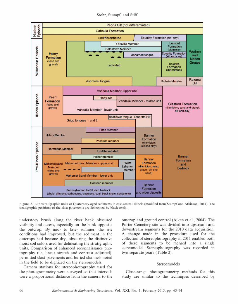
understory brush along the river bank obscuredvisibility and access, especially on the bank oppositethe outcrop. By mid- to late- summer, the siteconditions had improved, but the sediment in theoutcrops had become dry, obscuring the distinctivemoist soil colors used for delineating the stratigraphicunits. Comparison of enhanced reconnaissance pho-tography (i.e. linear stretch and contrast adjusted),permitted clast pavements and buried channels notedin the field to be digitized on the stereomodels.

Camera stations for stereophotography used forthe photogrammetry were surveyed so that intervalswere a proportional distance from the camera to the

outcrop and ground control (Aiken et al., 2004). ThePorter Cemetery site was divided into upstream anddownstream segments for the 2010 data acquisition.A change made in the procedure used for thecollection of stereophotography in 2011 enabled bothof these segments to be merged into a singlestereomodel. Stereophotography was recorded intwo separate years (Table 2).

Stereomodels

Close-range photogrammetry methods for thisstudy are similar to the techniques described by

Figure 2. Lithostratigraphic units of Quaternary-aged sediments in east-central Illinois (modified from Stumpf and Atkinson, 2014). Thestratigraphic positions of the clast pavements are delineated by black ovals.



Haneberg (2008), Poropat (2006), and Stohr et al.(2011). Photographs were taken with a tripod-mounted Nikon D80 camera (10.2 megapixels) anda Nikon 28-mm f/2 lens. A custom-made bracket witha clinometer and compass was used to ensure that thecamera orientation along three axes was consistent.

Creation of 3-D models and mosaics and determi-nation of georeferenced positions, feature delinea-tions, and other measurements were done using CAESirovisionTM software (version 4.1) developed by theAustralian Commonwealth Scientific and IndustrialResearch Organization (CSIRO) and CAE Mining.CAE Sirovision is a commercial close-range terrestrialdigital photogrammetry program created for geolog-ical and geotechnical mapping. The software consistsof two programs: Siro3D for 3-D model creation andSirojoint (version 5.0.18.0) for structural mappingand analysis.

Euclidean distances and summary statistics for allmeasurements were calculated using Microsoft OfficeExcelH software (version 2010). Computations ofprojected channel areas and perimeters were madeusing ArcMapTM Desktop software (version 10.1.1),a geographic information system and geodatabasemanagement system developed by the EnvironmentalSystems Research Institute (ESRI, Redlands, CA).Hugin freeware software (http://hugin.sourceforge.net/) and Adobe Photoshop (version 12.0.3) wereused to make uncontrolled mosaics (i.e., not geomet-rically corrected) for office use.

The location and distribution of individual cobble-sized clasts were determined by digitizing on geo-referenced stereomodels in Sirovision. Resolution andoverlap of individual images in the compositestereomodel required enhancement of the fieldphotographs for consultation to aid in identifying

Figure 3. Clast pavements and buried channel deposits in an outcrop at the Blue Hole site along the Middle Fork of the Vermilion River.Clasts are circled in blue in the Batestown Member till, in red in the Tiskilwa Formation till, and in green in unnamed sands of the GlasfordFormation and the Vandalia Member till. Clasts forming the pavement between the Batestown and Tiskilwa are circled in black. Solidorange, blue, green, and black lines represent formation boundaries. The buried channels within the upper unit of the Vandalia Member ofthe Glasford Formation are delineated with a stippled pattern, and the dashed lines indicate contacts that are covered or obscured. Thewhite sheets of paper are targets used as controls in the stereomodel.

Figure 4. Clast pavements and buried channel deposits in an outcrop at the Higginsville site along the Middle Fork of the Vermilion River.Clasts are circled in blue in the Batestown Member till, in red in the Tiskilwa Formation till, and in green in Unit 1 of the GlasfordFormation and Vandalia Member till. Clasts forming the pavement between the Batestown and Tiskilwa are circled in blue. Solid orange,blue, green, and black lines represent formational boundaries. The buried channels within the upper unit of the Vandalia Member of theGlasford Formation are delineated with a stippled pattern, and the dashed lines indicate contacts that are covered or obscured. Controlmarks are marked with orange paint. The white sheets of paper are targets used as controls in the stereomodel.



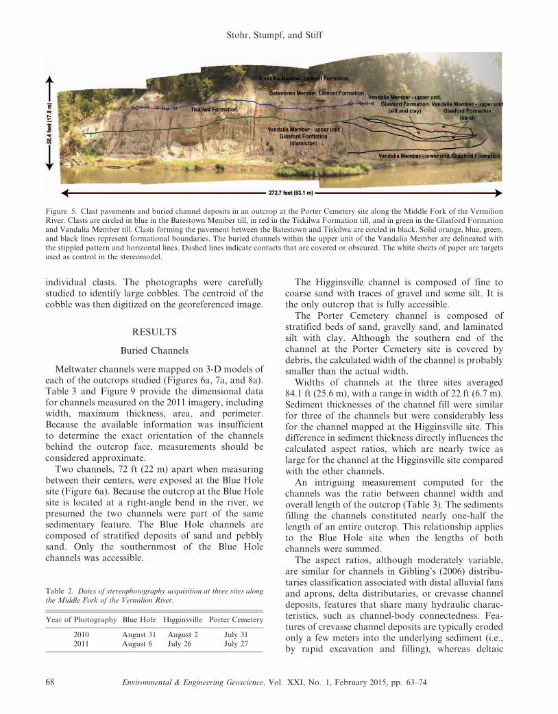
individual clasts. The photographs were carefullystudied to identify large cobbles. The centroid of thecobble was then digitized on the georeferenced image.

RESULTS

Buried Channels

Meltwater channels were mapped on 3-D models ofeach of the outcrops studied (Figures 6a, 7a, and 8a).Table 3 and Figure 9 provide the dimensional datafor channels measured on the 2011 imagery, includingwidth, maximum thickness, area, and perimeter.Because the available information was insufficientto determine the exact orientation of the channelsbehind the outcrop face, measurements should beconsidered approximate.

Two channels, 72 ft (22 m) apart when measuringbetween their centers, were exposed at the Blue Holesite (Figure 6a). Because the outcrop at the Blue Holesite is located at a right-angle bend in the river, wepresumed the two channels were part of the samesedimentary feature. The Blue Hole channels arecomposed of stratified deposits of sand and pebblysand. Only the southernmost of the Blue Holechannels was accessible.

The Higginsville channel is composed of fine tocoarse sand with traces of gravel and some silt. It isthe only outcrop that is fully accessible.

The Porter Cemetery channel is composed ofstratified beds of sand, gravelly sand, and laminatedsilt with clay. Although the southern end of thechannel at the Porter Cemetery site is covered bydebris, the calculated width of the channel is probablysmaller than the actual width.

Widths of channels at the three sites averaged84.1 ft (25.6 m), with a range in width of 22 ft (6.7 m).Sediment thicknesses of the channel fill were similarfor three of the channels but were considerably lessfor the channel mapped at the Higginsville site. Thisdifference in sediment thickness directly influences thecalculated aspect ratios, which are nearly twice aslarge for the channel at the Higginsville site comparedwith the other channels.

An intriguing measurement computed for thechannels was the ratio between channel width andoverall length of the outcrop (Table 3). The sedimentsfilling the channels constituted nearly one-half thelength of an entire outcrop. This relationship appliesto the Blue Hole site when the lengths of bothchannels were summed.

The aspect ratios, although moderately variable,are similar for channels in Gibling’s (2006) distribu-taries classification associated with distal alluvial fansand aprons, delta distributaries, or crevasse channeldeposits, features that share many hydraulic charac-teristics, such as channel-body connectedness. Fea-tures of crevasse channel deposits are typically erodedonly a few meters into the underlying sediment (i.e.,by rapid excavation and filling), whereas deltaic

Figure 5. Clast pavements and buried channel deposits in an outcrop at the Porter Cemetery site along the Middle Fork of the VermilionRiver. Clasts are circled in blue in the Batestown Member till, in red in the Tiskilwa Formation till, and in green in the Glasford Formationand Vandalia Member till. Clasts forming the pavement between the Batestown and Tiskilwa are circled in black. Solid orange, blue, green,and black lines represent formational boundaries. The buried channels within the upper unit of the Vandalia Member are delineated withthe stippled pattern and horizontal lines. Dashed lines indicate contacts that are covered or obscured. The white sheets of paper are targetsused as control in the stereomodel.

Table 2. Dates of stereophotography acquisition at three sites alongthe Middle Fork of the Vermilion River.

Year of Photography Blue Hole Higginsville Porter Cemetery

2010 August 31 August 2 July 312011 August 6 July 26 July 27



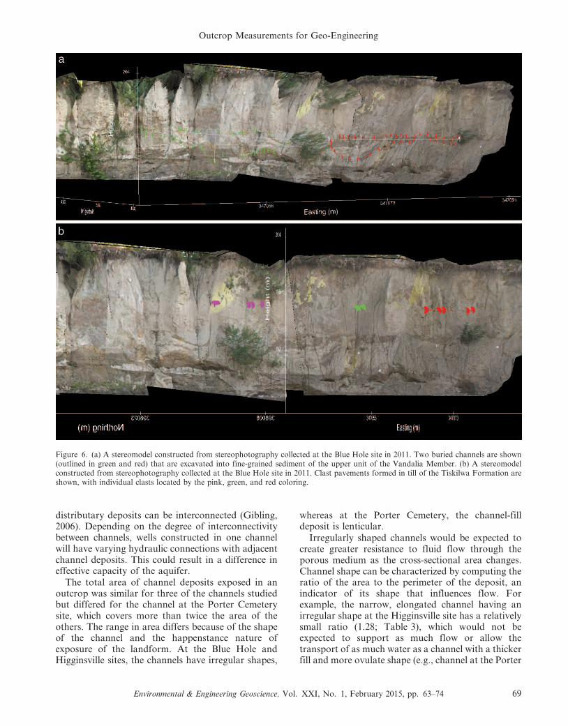
distributary deposits can be interconnected (Gibling,2006). Depending on the degree of interconnectivitybetween channels, wells constructed in one channelwill have varying hydraulic connections with adjacentchannel deposits. This could result in a difference ineffective capacity of the aquifer.

The total area of channel deposits exposed in anoutcrop was similar for three of the channels studiedbut differed for the channel at the Porter Cemeterysite, which covers more than twice the area of theothers. The range in area differs because of the shapeof the channel and the happenstance nature ofexposure of the landform. At the Blue Hole andHigginsville sites, the channels have irregular shapes,

whereas at the Porter Cemetery, the channel-filldeposit is lenticular.

Irregularly shaped channels would be expected tocreate greater resistance to fluid flow through theporous medium as the cross-sectional area changes.Channel shape can be characterized by computing theratio of the area to the perimeter of the deposit, anindicator of its shape that influences flow. Forexample, the narrow, elongated channel having anirregular shape at the Higginsville site has a relativelysmall ratio (1.28; Table 3), which would not beexpected to support as much flow or allow thetransport of as much water as a channel with a thickerfill and more ovulate shape (e.g., channel at the Porter

Figure 6. (a) A stereomodel constructed from stereophotography collected at the Blue Hole site in 2011. Two buried channels are shown(outlined in green and red) that are excavated into fine-grained sediment of the upper unit of the Vandalia Member. (b) A stereomodelconstructed from stereophotography collected at the Blue Hole site in 2011. Clast pavements formed in till of the Tiskilwa Formation areshown, with individual clasts located by the pink, green, and red coloring.



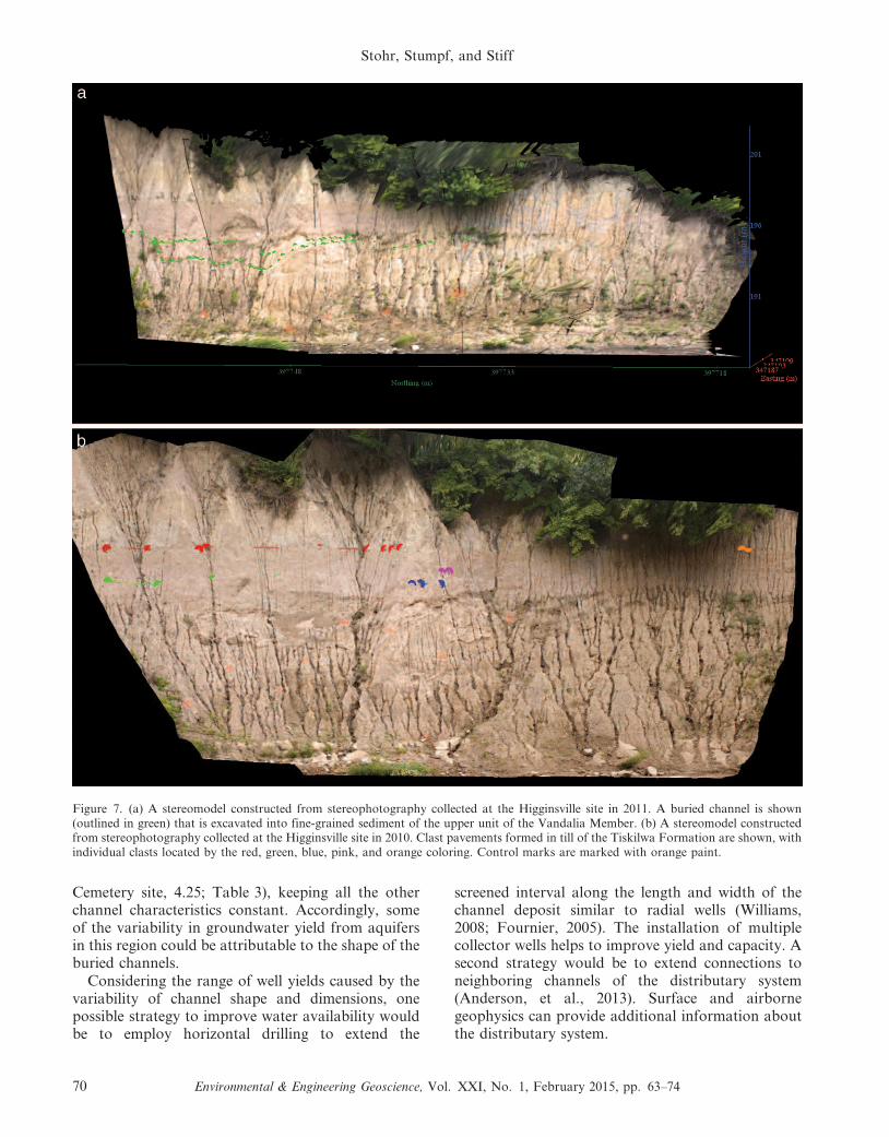
Cemetery site, 4.25; Table 3), keeping all the otherchannel characteristics constant. Accordingly, someof the variability in groundwater yield from aquifersin this region could be attributable to the shape of theburied channels.

Considering the range of well yields caused by thevariability of channel shape and dimensions, onepossible strategy to improve water availability wouldbe to employ horizontal drilling to extend the

screened interval along the length and width of thechannel deposit similar to radial wells (Williams,2008; Fournier, 2005). The installation of multiplecollector wells helps to improve yield and capacity. Asecond strategy would be to extend connections toneighboring channels of the distributary system(Anderson, et al., 2013). Surface and airbornegeophysics can provide additional information aboutthe distributary system.

Figure 7. (a) A stereomodel constructed from stereophotography collected at the Higginsville site in 2011. A buried channel is shown(outlined in green) that is excavated into fine-grained sediment of the upper unit of the Vandalia Member. (b) A stereomodel constructedfrom stereophotography collected at the Higginsville site in 2010. Clast pavements formed in till of the Tiskilwa Formation are shown, withindividual clasts located by the red, green, blue, pink, and orange coloring. Control marks are marked with orange paint.



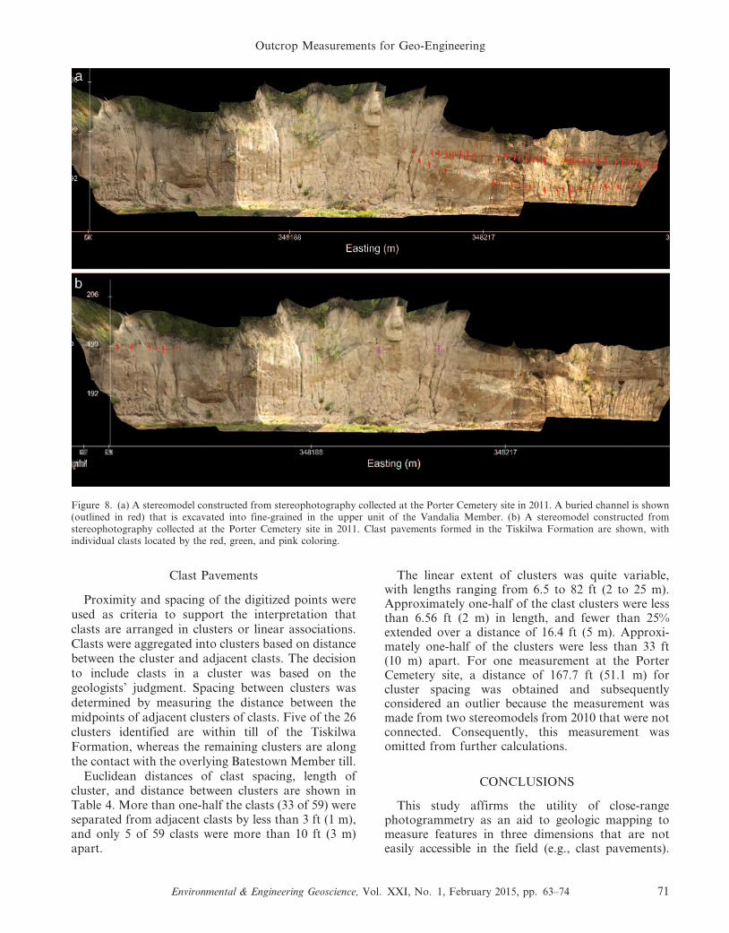
Clast Pavements

Proximity and spacing of the digitized points wereused as criteria to support the interpretation thatclasts are arranged in clusters or linear associations.Clasts were aggregated into clusters based on distancebetween the cluster and adjacent clasts. The decisionto include clasts in a cluster was based on thegeologists’ judgment. Spacing between clusters wasdetermined by measuring the distance between themidpoints of adjacent clusters of clasts. Five of the 26clusters identified are within till of the TiskilwaFormation, whereas the remaining clusters are alongthe contact with the overlying Batestown Member till.

Euclidean distances of clast spacing, length ofcluster, and distance between clusters are shown inTable 4. More than one-half the clasts (33 of 59) wereseparated from adjacent clasts by less than 3 ft (1 m),and only 5 of 59 clasts were more than 10 ft (3 m)apart.

The linear extent of clusters was quite variable,with lengths ranging from 6.5 to 82 ft (2 to 25 m).Approximately one-half of the clast clusters were lessthan 6.56 ft (2 m) in length, and fewer than 25%extended over a distance of 16.4 ft (5 m). Approxi-mately one-half of the clusters were less than 33 ft(10 m) apart. For one measurement at the PorterCemetery site, a distance of 167.7 ft (51.1 m) forcluster spacing was obtained and subsequentlyconsidered an outlier because the measurement wasmade from two stereomodels from 2010 that were notconnected. Consequently, this measurement wasomitted from further calculations.

CONCLUSIONS

This study affirms the utility of close-rangephotogrammetry as an aid to geologic mapping tomeasure features in three dimensions that are noteasily accessible in the field (e.g., clast pavements).

Figure 8. (a) A stereomodel constructed from stereophotography collected at the Porter Cemetery site in 2011. A buried channel is shown(outlined in red) that is excavated into fine-grained in the upper unit of the Vandalia Member. (b) A stereomodel constructed fromstereophotography collected at the Porter Cemetery site in 2011. Clast pavements formed in the Tiskilwa Formation are shown, withindividual clasts located by the red, green, and pink coloring.



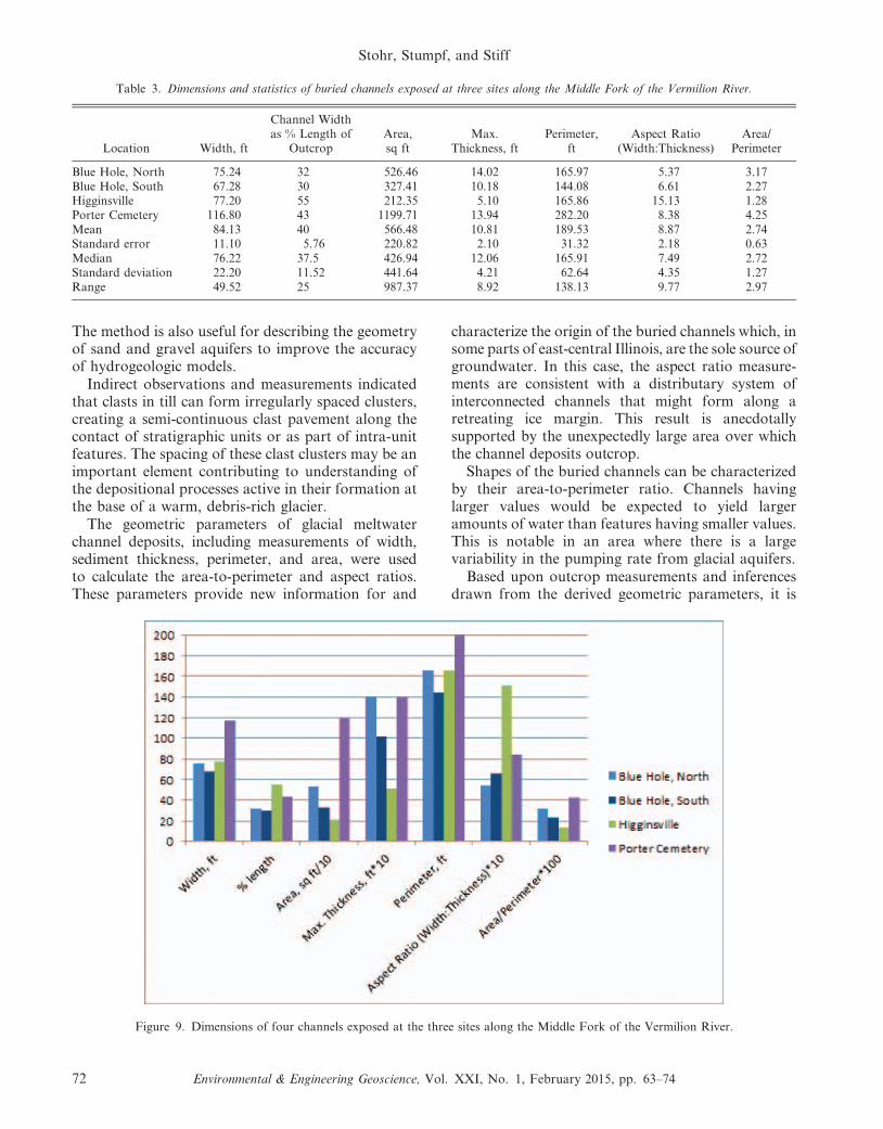
The method is also useful for describing the geometryof sand and gravel aquifers to improve the accuracyof hydrogeologic models.

Indirect observations and measurements indicatedthat clasts in till can form irregularly spaced clusters,creating a semi-continuous clast pavement along thecontact of stratigraphic units or as part of intra-unitfeatures. The spacing of these clast clusters may be animportant element contributing to understanding ofthe depositional processes active in their formation atthe base of a warm, debris-rich glacier.

The geometric parameters of glacial meltwaterchannel deposits, including measurements of width,sediment thickness, perimeter, and area, were usedto calculate the area-to-perimeter and aspect ratios.These parameters provide new information for and

characterize the origin of the buried channels which, insome parts of east-central Illinois, are the sole source ofgroundwater. In this case, the aspect ratio measure-ments are consistent with a distributary system ofinterconnected channels that might form along aretreating ice margin. This result is anecdotallysupported by the unexpectedly large area over whichthe channel deposits outcrop.

Shapes of the buried channels can be characterizedby their area-to-perimeter ratio. Channels havinglarger values would be expected to yield largeramounts of water than features having smaller values.This is notable in an area where there is a largevariability in the pumping rate from glacial aquifers.

Based upon outcrop measurements and inferencesdrawn from the derived geometric parameters, it is

Figure 9. Dimensions of four channels exposed at the three sites along the Middle Fork of the Vermilion River.

Table 3. Dimensions and statistics of buried channels exposed at three sites along the Middle Fork of the Vermilion River.

Location Width, ft

Channel Widthas % Length of

OutcropArea,sq ft

Max.Thickness, ft

Perimeter,ft

Aspect Ratio(Width:Thickness)

Area/Perimeter

Blue Hole, North 75.24 32 526.46 14.02 165.97 5.37 3.17Blue Hole, South 67.28 30 327.41 10.18 144.08 6.61 2.27Higginsville 77.20 55 212.35 5.10 165.86 15.13 1.28Porter Cemetery 116.80 43 1199.71 13.94 282.20 8.38 4.25Mean 84.13 40 566.48 10.81 189.53 8.87 2.74Standard error 11.10 5.76 220.82 2.10 31.32 2.18 0.63Median 76.22 37.5 426.94 12.06 165.91 7.49 2.72Standard deviation 22.20 11.52 441.64 4.21 62.64 4.35 1.27Range 49.52 25 987.37 8.92 138.13 9.77 2.97



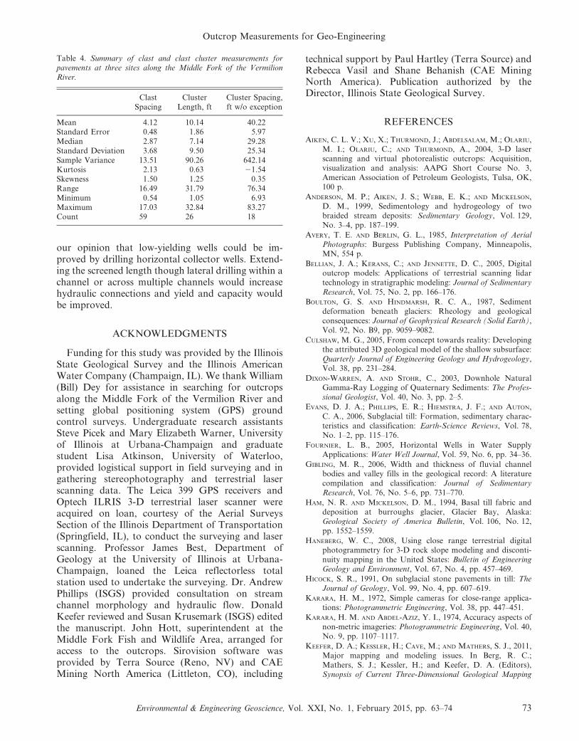
our opinion that low-yielding wells could be im-proved by drilling horizontal collector wells. Extend-ing the screened length though lateral drilling within achannel or across multiple channels would increasehydraulic connections and yield and capacity wouldbe improved.

ACKNOWLEDGMENTS

Funding for this study was provided by the IllinoisState Geological Survey and the Illinois AmericanWater Company (Champaign, IL). We thank William(Bill) Dey for assistance in searching for outcropsalong the Middle Fork of the Vermilion River andsetting global positioning system (GPS) groundcontrol surveys. Undergraduate research assistantsSteve Picek and Mary Elizabeth Warner, Universityof Illinois at Urbana-Champaign and graduatestudent Lisa Atkinson, University of Waterloo,provided logistical support in field surveying and ingathering stereophotography and terrestrial laserscanning data. The Leica 399 GPS receivers andOptech ILRIS 3-D terrestrial laser scanner wereacquired on loan, courtesy of the Aerial SurveysSection of the Illinois Department of Transportation(Springfield, IL), to conduct the surveying and laserscanning. Professor James Best, Department ofGeology at the University of Illinois at Urbana-Champaign, loaned the Leica reflectorless totalstation used to undertake the surveying. Dr. AndrewPhillips (ISGS) provided consultation on streamchannel morphology and hydraulic flow. DonaldKeefer reviewed and Susan Krusemark (ISGS) editedthe manuscript. John Hott, superintendent at theMiddle Fork Fish and Wildlife Area, arranged foraccess to the outcrops. Sirovision software wasprovided by Terra Source (Reno, NV) and CAEMining North America (Littleton, CO), including

technical support by Paul Hartley (Terra Source) andRebecca Vasil and Shane Behanish (CAE MiningNorth America). Publication authorized by theDirector, Illinois State Geological Survey.

REFERENCES

AIKEN, C. L. V.; XU, X.; THURMOND, J.; ABDELSALAM, M.; OLARIU,M. I.; OLARIU, C.; AND THURMOND, A., 2004, 3-D laserscanning and virtual photorealistic outcrops: Acquisition,visualization and analysis: AAPG Short Course No. 3,American Association of Petroleum Geologists, Tulsa, OK,100 p.

ANDERSON, M. P.; AIKEN, J. S.; WEBB, E. K.; AND MICKELSON,D. M., 1999, Sedimentology and hydrogeology of twobraided stream deposits: Sedimentary Geology, Vol. 129,No. 3–4, pp. 187–199.

AVERY, T. E. AND BERLIN, G. L., 1985, Interpretation of AerialPhotographs: Burgess Publishing Company, Minneapolis,MN, 554 p.

BELLIAN, J. A.; KERANS, C.; AND JENNETTE, D. C., 2005, Digitaloutcrop models: Applications of terrestrial scanning lidartechnology in stratigraphic modeling: Journal of Sedimentary

Research, Vol. 75, No. 2, pp. 166–176.

BOULTON, G. S. AND HINDMARSH, R. C. A., 1987, Sedimentdeformation beneath glaciers: Rheology and geologicalconsequences: Journal of Geophysical Research (Solid Earth),Vol. 92, No. B9, pp. 9059–9082.

CULSHAW, M. G., 2005, From concept towards reality: Developingthe attributed 3D geological model of the shallow subsurface:Quarterly Journal of Engineering Geology and Hydrogeology,Vol. 38, pp. 231–284.

DIXON-WARREN, A. AND STOHR, C., 2003, Downhole NaturalGamma-Ray Logging of Quaternary Sediments: The Profes-sional Geologist, Vol. 40, No. 3, pp. 2–5.

EVANS, D. J. A.; PHILLIPS, E. R.; HIEMSTRA, J. F.; AND AUTON,C. A., 2006, Subglacial till: Formation, sedimentary charac-teristics and classification: Earth-Science Reviews, Vol. 78,No. 1–2, pp. 115–176.

FOURNIER, L. B., 2005, Horizontal Wells in Water SupplyApplications: Water Well Journal, Vol. 59, No. 6, pp. 34–36.

GIBLING, M. R., 2006, Width and thickness of fluvial channelbodies and valley fills in the geological record: A literaturecompilation and classification: Journal of SedimentaryResearch, Vol. 76, No. 5–6, pp. 731–770.

HAM, N. R. AND MICKELSON, D. M., 1994, Basal till fabric anddeposition at burroughs glacier, Glacier Bay, Alaska:Geological Society of America Bulletin, Vol. 106, No. 12,pp. 1552–1559.

HANEBERG, W. C., 2008, Using close range terrestrial digitalphotogrammetry for 3-D rock slope modeling and disconti-nuity mapping in the United States: Bulletin of EngineeringGeology and Environment, Vol. 67, No. 4, pp. 457–469.

HICOCK, S. R., 1991, On subglacial stone pavements in till: TheJournal of Geology, Vol. 99, No. 4, pp. 607–619.

KARARA, H. M., 1972, Simple cameras for close-range applica-tions: Photogrammetric Engineering, Vol. 38, pp. 447–451.

KARARA, H. M. AND ABDEL-AZIZ, Y. I., 1974, Accuracy aspects ofnon-metric imageries: Photogrammetric Engineering, Vol. 40,No. 9, pp. 1107–1117.

KEEFER, D. A.; KESSLER, H.; CAVE, M.; AND MATHERS, S. J., 2011,Major mapping and modeling issues. In Berg, R. C.;Mathers, S. J.; Kessler, H.; and Keefer, D. A. (Editors),Synopsis of Current Three-Dimensional Geological Mapping

Table 4. Summary of clast and clast cluster measurements forpavements at three sites along the Middle Fork of the VermilionRiver.

ClastSpacing

ClusterLength, ft

Cluster Spacing,ft w/o exception

Mean 4.12 10.14 40.22Standard Error 0.48 1.86 5.97Median 2.87 7.14 29.28Standard Deviation 3.68 9.50 25.34Sample Variance 13.51 90.26 642.14Kurtosis 2.13 0.63 21.54Skewness 1.50 1.25 0.35Range 16.49 31.79 76.34Minimum 0.54 1.05 6.93Maximum 17.03 32.84 83.27Count 59 26 18



and Modeling in Geological Survey Organizations: IllinoisState Geological Survey Circular 578, pp. 5–10.

KEMPTON, J. P.; RINGLER, R. W.; HEIGOLD, P. C.; CARTWRIGHT, K.;AND POOLE, V. L., 1981, Groundwater Resources of NorthernVermilion County, Illinois: Illinois State Geological SurveyEnvironmental Geology Notes 101, 36 p.

LATO, M.; KEMENY, J.; HARRAP, R. M.; AND BEVAN, G., 2013,Rock bench: Establishing a common repository and stan-dards for assessing rockmass characteristics using LiDARand photogrammetry: Computers and Geosciences, Vol. 50,pp. 106–114.

MOFFITT, F. H. AND MIKHAIL, E. M., 1980, Photogrammetry, 3rded.: Harper and Row Publishers, New York, NY, 648 p.

POROPAT, G. V., 2006, Remote 3D mapping of rock massstructure. In Tonon, F. and J. Kottenstette, J. (Editors),Laser and Photogrammetric Methods for Rock Face Charac-terization Workshop: American Rock Mechanics Association,Alexandria, VA, pp. 63–75.

RABBEN, E. L.; CHALMERS, E. L., JR; MANLEY, E.; AND PICKUP, J.,1960, Fundamentals of photo interpretation. In Colwell,R. N. (Editor), Manual of Photographic Interpretation:American Society of Photogrammetry, Washington, DC,pp. 99–168.

SAUER, E. K., 1974, Geotechnical implications of Pleistocenedeposits in southern Saskatchewan: Canadian GeotechnicalJournal, Vol. 11, No. 3, pp. 359–373.

STOHR, C.; DIXON-WARREN, A.; KEITH, K.; KOENIG, S.; BARN-

HARDT, M.; CURRY, B.; STUMPF, A.; HANSEL, A.; BHAGWAT, S.;DUVAL, J.; AND KORTH, D., 2004, Downhole, NaturalGamma Logging for Engineering & Environmental Applica-tions of Quaternary Geology Mapping: 47th Annual Meetingof the Association of Engineering Geologists: DearbornMichigan (September 26–October 1, 2004), Program withAbstracts, pp. 54–55.

STOHR, C. J.; PETRAS, J.; MIKULIC, D. G.; AND THOMASON, J.,2011, Stereophotographic Measurement of Joint and Bedding

Orientation at Thornton Quarry, Illinois: Illinois StateGeological Survey Circular 579, 23 p. and seven appendices.Electronic document available at http://library.isgs.uiuc.edu/Pubs/pdfs/circulars/c579.pdf

STUMPF, A. J. AND ATKINSON, L. A., 2014, Cross sections of thegeology over the Mahomet Bedrock Valley in east-centralIllinois. Ill State Geological Survey Illinois Map 19.

STUMPF, A. J. AND DEY, W. S., editors, (in review), Understandingthe Mahomet Aquifer: Geological, Geophysical, and Hydro-geological Studies in Champaign County and Adjacent Areas:Illinois State Geological Survey, Draft Contract ReportIllinois American Water 2007-02899.

VOORHEES, D. H., 1996, Evidence and implications of a stone bedof a subglacial fluvial origin in east central Illinois. InProgram with Abstracts: Geological Society of America,Denver, CO, Vol. 28, No. 7, p. A111.

VOORHEES, D. H., 1998, Stone Bed Sedimentology and Petrographyof Wisconsinan Tills Used to Infer Subglacial Bed Conditionsin Northern Illinois: Unpublished Manuscript, Illinois StateGeological Survey, 355 p.

WHITMEYER, S. J.; FEELY, M.; DE PAOR, D. G.; HENNESSY, R.;WHITMEYER, S.; NICOLETTI, J.; SANTANGELO, B.; DANIELS, J.;AND RIVERA, M., 2009, Visualization techniques in fieldgeology education: A case study from western Ireland. InWhitmeyer, S. J.; Mogk, D.; and Pyle, E. J. (Editors), FieldGeology Education: Historical Perspectives and ModernApproaches: Geological Society of America Special Paper461, pp. 105–115. Electronic document available at http://dx.doi.org/10.1130/2009.2461(10)

WILLIAMS, D. E., 2008, Research and Development for Horizontal/Angle Well Technology: U.S. Department of the Interior,Bureau of Reclamation, Denver, CO, 77 p.

XU, X.; AIKEN, C. L.; BHATTACHARYA, J. P.; CORBEANU, R. M.;NIELSEN, K. C.; MCMECHAN, G. A.; AND ABDELSALAM, M. G.,2000, Creating virtual 3-D outcrop: The Leading Edge,Vol. 19, No. 2, pp. 197–202.



Documents

Environmental & Engineering Geoscience