Environment and productivities in developed and developing countries: The case of carbon dioxide and sulfur dioxide

lable at ScienceDirect

Journal of Environmental Management 91 (2010) 1580e1592

Contents lists avai

Journal of Environmental Management

journal homepage: www.elsevier .com/locate/ jenvman

Environment and productivities in developed and developing countries: The caseof carbon dioxide and sulfur dioxide

Surender Kumar a, Shunsuke Managi b,c,*aDepartment of Policy Studies, TERI University, 10, Institutional Area, Vasant Kunj, New Delhi 110070, IndiabGraduate School of Environmental Studies, Tohoku University, 6-6-20 Aramaki-Aza Aoba, Aoba-Ku, Sendai 980-8579, Japanc Institute for Global Environmental Strategies, Japan

a r t i c l e i n f o

Article history:Received 21 April 2009Received in revised form5 December 2009Accepted 10 March 2010Available online 10 April 2010

JEL classification:Q55O30

Keywords:Environmental efficiencyProductivitySemi-parametric estimation

* Corresponding author. Graduate School of EnvUniversity, 6-6-20 Aramaki-Aza Aoba, Aoba-Ku, Send45 339 3751; fax: þ81 45 339 3707.

E-mail address: [email protected] (S. Managi).1 Although the turning point has been identified fo

still considerable uncertainty with respect to those inenvironmental harm associated with the turningbehind the EKC (Verbeke and De Clercq, 2002). Thepioneering study by Grossman and Krueger (1993).and Krueger (1993), many studies such as SeldenEakin and Selden (1995) investigated this relationshienvironmental degradation with levels of pollutantsa summary of the recent literature, see Stern, 2004;Managi, 2006).

0301-4797/$ e see front matter � 2010 Elsevier Ltd.doi:10.1016/j.jenvman.2010.03.003

a b s t r a c t

We propose a productivity index for undesirable outputs such as carbon dioxide (CO2) and sulfur dioxide(SO2) emissions and measure it using data from 51 developed and developing countries over the period1971e2000. About half of the countries exhibit the productivity growth. The changes in the productivityindex are linked with their respective per capita income using a semi-parametric model. Our resultsshow technological catch up of low-income countries. However, overall productivities both of SO2 andCO2 show somewhat different results.

� 2010 Elsevier Ltd. All rights reserved.

1. Introduction

The environmental Kuznets curve (EKC) hypothesis has gener-ated a vast number of studies to examine the existence of aninverted ‘U’-shaped relationship between income and environ-mental degradation, and the literature is far from conclusive.1 Aftera certain level of income, concern for environmental degradationbecomes more relevant and a mechanism to reduce environmentaldegradation is put in place through necessary institutional, legal,and technological adjustments (e.g., Grossman and Krueger, 1995).

ironmental Studies, Tohokuai 980-8579, Japan. Tel.: þ81

r various pollutants, there iscome levels, the peak level ofpoint, and the mechanismsEKC draws its roots from theAfter the study by Grossmanand Song (1994) and Holtz-p for alternative measures ofor pollutant intensities (forDeacon and Norman, 2006;

All rights reserved.

However, one of the major criticisms against these studies isthat they have adopted a reduced form approach to examine therelationship between per capita income and pollution emissions(see Stern, 1998; Dinda, 2004, for detailed discussions on majorproblems in the EKC). These two variables are merely the outcomesof a production process, but they do not explain the underlyingproduction process, which converts inputs into outputs andpollutants. In fact, the transformation of this production processmay lead to environmental improvement at a higher level ofincome (Zaim and Taskin, 2000). Therefore, studies that examinethe transformation of production processes by quantifying theopportunity cost of adopting alternative environmentally superiortechnologies are more relevant to understanding the process ofpollution management and, therefore, to our study.

Some of the current income differences among countries are theoutcome of what happened to total factor productivity (TFP)subsequent to the beginning of modern economic growth (Prescott,1998). Similarly, differences in TFP have important implications forenvironmental quality (Chimeli and Braden, 2005). Therefore, it isimportant to understand TFP with regard to environmental perfor-mance and technology. More efficient utilization of pollutionabatement technologies, at least in part, influences the cost ofalternative production and pollution abatement technologies (e.g.,Jaffe et al., 2003; Managi, 2004). An extensive body of theoretical

mailto:[email protected]

www.sciencedirect.com/science/journal/03014797

http://www.elsevier.com/locate/jenvman

S. Kumar, S. Managi / Journal of Environmental Management 91 (2010) 1580e1592 1581

literature examines the role of environmental policy in encouraging(or discouraging) productivity growth. On the one hand, abatementpressuresmay stimulate innovative responses that reduce the actualcost of compliance below those originally estimated. On the otherhand, firms may be reluctant to innovate if they believe regulatorswill respond by ‘ratcheting-up’ standards even further. Therefore, inaddition to the changes in environmental regulations and tech-nology, management levels also affect the intertemporal environ-mental performance level. Thisperformance is calledenvironmentalproductivity (EP), which explains how efficiently pollutions aretreated (Managi et al., 2005). Thus, whether EP increases over timeand in a higher income range is an empirical question.

We are interested in whether there are any relationshipsbetween income and intertemporal environmental performance inthe spirit of the EKC. The objective of this paper is as follows. First,we measure productivity change for environmental (nonmarket)outputs such as carbon dioxide (CO2) and sulfur dioxide (SO2)emissions using country-level data for 51 developed and deve-loping countries over the period 1971e2000. We measure EPextending the TFP literature (see Färe et al., 2005; Managi et al.,2005). During our study period when public policies and publicconcern for global warming were minimal, we examine business-as-usual trends in costs of abatement and EP in CO2.2 In the case oflocal pollution of SO2, environmental policies have been imple-mented and therefore higher EP is expected if regulations areimplemented effectively. Then, the changes in EP in differentcountries are linked with their respective per capita income toexamine an EKC-type relationship. We then discuss the implica-tions for developed and developing countries.

The remainder of the paper is organized as follows: In Section 2,we discuss the empirical strategy and review the literature. Section3 describes the efficiency and productivity estimation models, andsemi-parametric estimation of an EKC-type relationship. Data usedin the study and results are presented and discussed in Section 4.The paper closes in Section 5 with some concluding remarks.

2. Empirical strategy

In the absence of direct data on the abatement costs and price ofemissions at the country level, we rely on a distance functionapproach that incorporates both the desirable output (grossdomestic product, GDP) and undesirable output such as CO2 andSO2 to measure ‘how far’ each country’s output vector is from thebest-practice frontier, for a given input vector. This approachrecognizes that pollution is an undesirable output that is not freelydisposable; rather it is weakly disposable. That is, some productiveresources have to be given up in order to reduce the pollution. Theextent to which a country would need to sacrifice its desirableoutput to reduce pollution represents its opportunity cost of

2 One of the important implications of global warming and increased CO2

emissions and growing global concern (and one of the causes of political concern) isthe impact on agriculture. The potential for dramatically disparate implications ofglobal warming and the impact of rising CO2 emissions by agricultural sector bycountry matter in determining winners and losers. Previous research on climatechange effect on agriculture is inconclusive about the sign and magnitude of itseffect (see, for example, Schlenker et al., 2006; Edgerton, 2009). Schlenker et al.(2006) identify major yield losses due to global warming in the corn sector,while Edgerton (2009) argues that CO2 increases consistent with global warmingwill boost corn yields. This suggests more work on CO2 as a factor of production inworld agriculture (see Ball et al. (2002)) and and a more careful analysis of winnersand losers at a subsector level is warranted. In our summary of country-levelanalysis of CO2 emissions is where the action is and where interpretable infor-mation can be developed. Sectoral analysis is beyond the scope of our paper, and weleave it for future research (See the subsector levels (e.g. Managi et al. (2005) focuson the oil and gas industry).

pollution reduction. We use the term environmental efficiency (EE)as a static notion of environmental performance measurement toestimate the opportunity cost following the production frontierliterature (see Färe et al., 2005). Less constrained firms areconsidered to be more environmentally efficient because they havechosen a more appropriate mix of desirable outputs, undesirableoutputs, and inputs, and would potentially find it less costly toreduce pollution.

We examine the trends in TFP3 for individual countries underthe assumption that emissions are weakly disposable and comparethese estimates with the conventional measures of productivitythat ignore the generation of these emissions.4 The ratio of thesetwo estimates of TFP provides a measure of the EP of a country,which can be interpreted as the intertemporal efficiency showinghowwell environmentally friendly technologies andmanagementsare utilized (e.g., Jaffe et al., 2003). EE and EP are two different waysto measure the effects of emission abatement. While EE is a staticmeasure of a country’s ability to increase GDP under the constraintof meeting emission reduction targets at a point in time, EP isa measure of the effect of those targets on a country’s ability tomove towards the best-practice frontier and to shift the frontierover time. EP can be considered as an extendedmeasure of TFP thatcredits activities reducing emissions. It provides a measure of theextent to which countries are becoming more efficient over time byincreasing desirable outputs while reducing undesirable outputs.We show that EE at a point in time is one of the several componentsof EP and that the two are not perfectly correlated.

There are several studies on the measurement of efficiencyand productivity changes in industries that produce desirableand undesirable outputs simultaneously during the productionprocess. Some of these studies have treated the undesirableoutputs as inputs,5 while others treated them as a syntheticoutput such as pollution abatement (e.g., Gollop and Roberts,1983). The approach adopted by Gollop and Roberts to treatthe reduction in undesirable output as desirable output createsa different nonlinear transformation of the original variable inthe absence of base constrained emission rates (Atkinson andDorfman, 2005). To overcome this problem, Pittman (1983)proposed that desirable and undesirable outputs should betreated nonsymmetrically. Following Chung et al. (1997) andYoruk and Zaim (2005), we use the directional output distancefunction to calculate production relationships involving desirableand undesirable outputs while treating them asymmetrically.

Several studies used the distance function approach to estimatethe country-level EE of CO2 to test EKC-type relationships. Thesestudies include Zaim and Taskin (2000), Zofio and Prieto (2001),and Taskin and Zaim (2001). The first two studies focused on theestimation of EE in OECD countries while the third study examinedthe effect of international trade on EE for a sample of 49 developed

3 Studies measuring TFP using the average production function assume thata firm is operating on its production frontier (e.g., Pittman, 1981; Murty and Kumar,2004). These studies treat TFP analogous to technological change.

4 Conventional measure of productivity ignores the generation of pollutants andonly considers good outputs and conventional inputs. It differs from themeasurement of productivity under the strong disposability of emissionsassumption. Productivity measurement assuming strong disposability of emissionsconsiders all good and bad outputs with conventional inputs, and bad outputs aretreated alike good outputs. That is, ignoring bad outputs is not equivalent to strongdisposability. In the DEA analysis strong disposability means emissions are includedin the analysis but modeled with an inequality sign.

5 See Pittman (1981), Cropper and Oates (1992), Kopp (1998), Reinhard et al.(1999), and Murty and Kumar (2004). Also see Kortelainen (2008) for review inthis literature.

7 Hailu and Veeman (2001) and Ebert and Welsch (2007) propose using emis-sions as inputs. However, Färe and Grosskopf (2003) show that it is inconsistentwith physical laws since it allows for the production of an unbounded amount ofundesirable outputs with given inputs and that instead of crediting firms forreducing bad outputs. It involves crediting them for producing the same good andbad outputs with fewer inputs. Though, the approach suggested by Ebert andWelsch (2007) satisfies the material balance condition, but it also producesambiguous results as it does not credit the firms for reducing emissions.Kuosmanen (2005) questions the conventional way in which weak disposability isspecified and shows how weakly disposable technology can be modeled such that

S. Kumar, S. Managi / Journal of Environmental Management 91 (2010) 1580e15921582

and developing countries over the period 1977e1990.6 The firsttwo studies find a U-shaped EKC exists between EE and per capitaincome among OECD countries. Taskin and Zaim (2001) found thisto be the case for high-income countries, but that an inverseU-shaped relationship occurred for low- and middle-incomecountries. They also found that increasing openness of a countryabove a threshold level increases EE among the high-incomecountries, but does not have a significant impact on EE of low- andmiddle-income countries. We test the EKC-type relationship of GDPper capita and environmental performances of EE and EP of CO2 andSO2 in this paper. Compared with previous studies, our study hasseveral advantages. We use more data and also analyze SO2 and EPin addition to EE. Themeasure of EP has the additional advantage ofbeing a measure of intertemporal performance. That is, EP isdecomposed into technological change and efficiency changemeasurements. Technological change measures shifts in the fron-tier pollution abatements. Efficiency change measures change inthe position of a production unit relative to the frontier, so-called‘catching up’. Developed countries usually develop and applyadvanced technologies. Therefore, they are expected to have fastertechnological change while developing countries may be catchingup to the frontier and thus the efficiency change might be high. Theoverall relationship to income, which is a sum of technological andefficiency changes, may not be clear and it is an empirical question.Therefore, we believe we are able to obtain a better understandingof environmental performance.

Traditionally, parametric functional forms (of quadratic andcubic polynomials) of the relationship betweenper capita emissionsand per capita real GDP have been used in the literature to examinethe existence of the EKC. Although there is abundant literature ontheEKC, its econometric applications havebeen criticized because ofa lack of robust econometric methods (Stern, 2004). Recently, inresponse to these claims, semi-parametric specifications have beenused to reexamine these results because it is more flexible thanpopular parametric functional forms (see Azomahou et al., 2006). Inthis study, we use semi-parametric estimation of generalized addi-tive models, which has not yet been applied in the EKC literature. Incomparison with previous nonparametric methods, this techniquehas the advantage of overcoming the difficulty of includingmultipleindependent variables into semi-parametric specifications.

3. Model

3.1. Measurement of EE and EP

Suppose that a country employs a vector of inputs x˛<Kþ toproduce a vector of desirable outputs y˛<Mþ , and undesirableoutputs b˛<Nþ. Let P(x) be the feasible output set for the given inputvector x and L(y, b) be the input requirement set for a given outputvector (y, b). Now the technology set is defined as:

T¼ {(y, b, x): x can produce (y, b)} (1)

The technology is modeled in alternative ways. The output isstrongly (or freely) disposable if (y, b)˛ P(x) and (y0, b0)� (y, b)0(y0, b0)˛ P(x). This implies that if an observed output vector isfeasible, then any output vector smaller than that is also feasible.This assumption excludes production processes that generateundesirable outputs that are costly to dispose. For example,

6 The EKC-related pollution and GDP per capita is expected to have an invertedU-shape relationship. One would therefore expect the relationship between(1� EE) and GDP per capita to be an inverted U-shape, and that the relationshipbetween EE and GDP per capita would be a mirror image. Therefore, it would be U-shaped as well.

concerns about SO2 and greenhouse gases imply that these shouldnot be considered to be freely disposable. In such cases, undesirableoutputs are considered as being weakly disposable: (y, b)˛ P(x) and0� q� 10 (qy, qb)˛ P(x). This implies that pollution is costly todispose and abatement activities would typically divert resourcesaway from the production of desirable outputs and thus lead tolower levels of desirable outputs with given inputs.7

A functional representation of the technology is provided by thedirectional output distance function, which also providesa measure of inefficiency. The directional distance function seeks toincrease the desirable outputs whilst simultaneously reducing theundesirable outputs. Formally, the directional distance function8 isdefined as:

D!

oðy;b; x; gÞ ¼ supfb : ðy;bÞ þ bg˛PðxÞg; (2)

where g is the vector of directions in which outputs can be scaled.Following Chung et al. (1997), the direction taken is g¼ (y, �b),such that as the desirable outputs are increased the undesirableoutputs are decreased.

3.1.1. Environmental efficiencyFäre et al. (1996) assumes separability between desirable and

undesirable outputs, and Färe et al. (1995) assumes separabilitybetween outputs and attributes. Both studies use input distancefunctions as an analytical tool. Following these studies, we assumethat the directional output distance function is separable in desir-able and undesirable outputs9:

D!t

o

�yt;bt;xt

�¼ B

�bt�D_�!t

o�yt;xt

�; (3)

where D_�!t

oðyt; xtÞ ¼ supfb : ðxt ; yt þ bgÞ˛T_ g and T

_ ¼ fðyt; xtÞ :xt can produce ytg.

The set T_

is a technology set restricted to the production ofdesirable outputs, but without any consideration of undesirableoutputs bt . Therefore, with this assumption one can decomposetechnical inefficiency into the factors that reflect the influence of

‘pure’ technical inefficiency, D_�!t

oðyt ; xtÞ and the effect of undesir-

able outputs, BðbtÞ. Thus, EE is defined as:

EE ¼�1þ D

!ti

�yt ;bt ; xt

��.�1þ D

_�!t

i�yt ;xt

��: (4)

EE represents the extent to which a country would be con-strained in increasing outputs by its potential to transfer itsproduction process from free disposability to costly disposability ofthe emissions. Countries that are less constrained have a loweropportunity cost of transfer in the production process and are

non-uniform abatement factors can be applied across firms.8 For the properties of directional distance functions, see Färe et al. (2005).9 As the production of bad outputs cannot be separated out from the production

of good output, it is a very strong assumption. Wossink et al. (2001) outlines thelimitation of taking the assumption of separability. As the objective of present studyis to measure environmental efficiency and productivity, to separate out the effectof environment it is essential to take the assumption.


considered to be more environmentally efficient. That is, ifa country can produce the same level of desirable output with thegiven inputs under different disposability assumption, it impliesthat the country is not constrained by the weak disposability of badoutputs and it termed as environmentally efficient, thus highervalues of EE indicate higher environmental performance.

It is important to note that environmental efficiency of input oroutput-oriented distance functions might provide ambiguousresults. For example, in input-oriented environmental efficiencymeasure proposed by Färe et al. (1996), some results may revealthe counter-intuitive result such that one firm is identified as the“best observed environmental practice” even though it producesthe largest amount of undesirable output both in absolute scale

MLtþ1t ¼

ffiffiffiffiffiffiffiffiffiffiffiffiffiffiffiffiffiffiffiffiffiffiffiffiffiffiffiffiffiffiffiffiffiffiffiffiffiffiffiffiffiffiffiffiffiffiffiffiffiffiffiffiffiffiffiffiffiffiffiffiffiffiffiffiffiffiffiffiffiffiffiffiffiffiffiffiffiffiffiffiffiffiffiffiffiffiffiffiffiffiffiffiffiffiffiffiffiffiffiffiffiffiffiffiffiffiffiffiffiffiffiffiffiffiffiffiffiffiffiffiffiffiffiffiffiffiffiffiffin1þ D

!tþ1o

�yt ;bt ; xt

�on1þ D

!tþ1o

�ytþ1;btþ1; xtþ1

�o�n1þ D

!to

�yt ;bt ; xt

�on1þ D

!to


�ovuuuut ; (6a)

MLtþ1t ¼

" n1þ D

!to

�yt ;bt

; xt�o

n1þ D

!tþ1o

�ytþ1;btþ1

; xtþ1�o

#|fflfflfflfflfflfflfflfflfflfflfflfflfflfflfflfflfflfflfflfflfflfflfflfflfflfflfflfflfflfflffl{zfflfflfflfflfflfflfflfflfflfflfflfflfflfflfflfflfflfflfflfflfflfflfflfflfflfflfflfflfflfflffl}

MLEC

�

ffiffiffiffiffiffiffiffiffiffiffiffiffiffiffiffiffiffiffiffiffiffiffiffiffiffiffiffiffiffiffiffiffiffiffiffiffiffiffiffiffiffiffiffiffiffiffiffiffiffiffiffiffiffiffiffiffiffiffiffiffiffiffiffiffiffiffiffiffiffiffiffiffiffiffiffiffiffiffiffiffiffiffiffiffiffiffiffiffiffiffiffiffiffiffiffiffiffiffiffiffiffiffiffiffiffiffiffiffiffiffiffiffiffiffiffiffiffiffin1þ D

!tþ1o

�yt ;bt

; xt�o

n1þ D

!to

�yt ;bt ; xt

�o �n1þ D

!tþ1o

�ytþ1;btþ1

; xtþ1�o

n1þ D

!to


�ovuuuut|fflfflfflfflfflfflfflfflfflfflfflfflfflfflfflfflfflfflfflfflfflfflfflfflfflfflfflfflfflfflfflfflfflfflfflfflfflfflfflfflfflfflfflfflfflfflfflfflfflfflfflfflfflfflfflfflfflffl{zfflfflfflfflfflfflfflfflfflfflfflfflfflfflfflfflfflfflfflfflfflfflfflfflfflfflfflfflfflfflfflfflfflfflfflfflfflfflfflfflfflfflfflfflfflfflfflfflfflfflfflfflfflfflfflfflfflffl}

MLTC

; (6b)

and per unit of output. However, the directional output distancefunction as applied in this study is able to provide unambiguousresults.

3.1.2. Environmental productivityFäre et al. (1995) assume separability between outputs and

attributes and construct the productivity associatedwith attributes.In a similar manner, EP using a directional distance function isdefined as:

MLtþ1t ¼

ffiffiffiffiffiffiffiffiffiffiffiffiffiffiffiffiffiffiffiffiffiffiffiffiffiffiffiffiffiffiffiffiffiffiffiffiffiffiffiffiffiffiffiffiffiffiffiffiffiffiffiffiffiffiffiffiffiffiffiffiffiffiffiffiffiffiffiffiffiffiffiffiffiffiffiffiffiffiffiffiffiffiffiffiffiffiffiffiffiffiffiffiffiffiffiffiffiffiffiffiffiffiffiffiffiffiffiffiffiffiffiffiffiffiffiffiffiffiffiffiffiffiffiffiffiffiffiffiffiffiffiffiffiffiffiffiffiffiffiffiffiffiffiffiffiffiffiffiffiffiffiffiffiffiffiffiffiffiffiffiffiffiffiffiffiffiffiffiffiffiffiffiffiffiffiffiffiffiffiffiffiffiffiffiffiffiffiffiffiffiffiffiffiffiffiffiffiffiffiffiffiffiffiffiffiffiffiffiffiffiffiffiffiffiffiffiffiffiffiffiffiffiffiffiffiffiffiffiffiffiffiffiffiffiffiffiffiffiffiffiffiffiffiffiffiffiffiffiffiffin1þ D

!tþ1o

�yt ;bt ; xt

�on1þ D

!tþ1o


�o�n1þ D

!to

�yt ;bt ; xt

�on1þ D

!to


�o�n1þ D

!tþ1o

�ytþ1;bt ; xtþ1

�on1þ D

!tþ1o

�ytþ1;bt ; xtþ1

�o�n1þ D

!to

�yt ;btþ1;xt

�on1þ D

!to

�yt ;btþ1;xt

�ovuuuut

¼ EPtþ1t �

ffiffiffiffiffiffiffiffiffiffiffiffiffiffiffiffiffiffiffiffiffiffiffiffiffiffiffiffiffiffiffiffiffiffiffiffiffiffiffiffiffiffiffiffiffiffiffiffiffiffiffiffiffiffiffiffiffiffiffiffiffiffiffiffiffiffiffiffiffiffiffiffiffiffiffiffiffiffiffiffiffiffiffiffiffiffiffiffiffiffiffiffiffiffiffiffiffiffiffiffiffiffiffiffiffiffiffiffiffiffiffiffiffiffiffiffiffiffiffiffiffiffiffiffiffin1þ D

!to

�yt ;btþ1

; xt�o

n1þ D

!to


�o�n1þ D

!tþ1o

�yt ;bt

; xt�o

n1þ D

!tþ1o

�ytþ1;bt ; xtþ1

�ovuuuut ;

(7)

EPtþ1t ¼

ffiffiffiffiffiffiffiffiffiffiffiffiffiffiffiffiffiffiffiffiffiffiffiffiffiffiffiffiffiffiffiffiffiffiffiffiffiffiffiffiffiffiffiffiffiffiffiffiffiffiffiffiffiffiffiffiffiffiffiffiffiffiffiffiffiffiffiffiffiffiffiffiffiffiffiffiffiffiffiffiffiffiffiffiffiffiffiffiffiffiffiffiffiffiffiffiffiffiffiffiffiffi1þ D

!to

�yt ;bt ;xt

�1þ D

!to

�yt ;btþ1;xt

�� 1þ D!tþ1

o

�ytþ1;bt ;xtþ1

�1þ D

!tþ1o

�ytþ1;btþ1;xtþ1

�vuuuut : (5)

EP depends on three parameters in addition to the value of badoutputs, the production technology represented by the directionaloutput distance function in two periods, the values of inputs andoutputs at these two points of time, whichmakes the value of EP anintegrated part of the production process. Note that EP measuresthe intertemporal environmental performance, which is based onthemixed period values of the directional output distance function.The EP index is the geometric mean of two ratios of directional

distance functions: the first takes period t as a reference and thesecond takes period tþ 1 as its reference point. The index EPtþ1

provides a direct measure of changes in environmental perfor-mance over time t.

As explained above, we assume that the technology admitsstrong disposability of desirable outputs and weak disposability of

undesirable outputs, so that if btþ1 < bt , D!t

oðyt ;btþ1; xtÞ �D!t

oðyt ;bt ; xtÞ and D!tþ1

o ðytþ1;btþ1; xtþ1Þ � D!tþ1

o ðytþ1;bt ; xtþ1Þ.Hence, if less pollution is produced in the next year, the index valueis greater than or equal to one, i.e., EP � 1.

Chung et al. (1997) defined the MalmquisteLuenberger (ML)index between periods t and tþ 1 as:

which can be further decomposed as:

where the first term, MLEC, represents the efficiency changecomponent, a movement towards the best-practice frontier or‘catch up’ to the frontier, while the second term, MLTC, is techno-logical change. Technological change explains how the frontieritself can shift over time.

In order to illustrate the relationship between the EP index of Eq.(5) and the ML index of Eq. (6), we note by introducing

1þ D!t

oðyt ; btþ1; xtÞ and 1þ D!tþ1

o ðytþ1; bt ; xtþ1Þ twice into Eq. (6)that:

i.e., the ML index can be written as a product of the EP index anda measure of productivity for a given level of undesirable outputvector. We note that if the undesirable output vector is dropped(using the assumption of separability between desirable andundesirable outputs) or emissions are freely disposable, the termin the root of Eq. (7) is the conventional measure of productivity(MS), i.e.:

MS ¼

ffiffiffiffiffiffiffiffiffiffiffiffiffiffiffiffiffiffiffiffiffiffiffiffiffiffiffiffiffiffiffiffiffiffiffiffiffiffiffiffiffiffiffiffiffiffiffiffiffiffiffiffiffiffiffiffiffiffiffiffiffiffiffiffiffiffiffiffiffiffiffiffiffiffiffiffiffiffiffiffiffiffiffiffiffiffiffiffiffiffiffiffiffiffiffiffiffiffiffiffiffiffi�1þ D

!to�yt ;xt

��1þ D

!to�ytþ1;xtþ1

��n1þ D

!tþ1o

�yt ;xt

�on1þ D

!tþ1o

�ytþ1;xtþ1

�ovuuuut ; (8a)


which can be further decomposed into two componentmeasures ofproductivity change:

MStþ1t ¼

" �1þ D

!to�yt ;xt

�n1þ D

!tþ1o

�ytþ1;xtþ1

�o#

|fflfflfflfflfflfflfflfflfflfflfflfflfflfflfflfflfflfflfflfflfflfflfflffl{zfflfflfflfflfflfflfflfflfflfflfflfflfflfflfflfflfflfflfflfflfflfflfflffl}MSEC

�

ffiffiffiffiffiffiffiffiffiffiffiffiffiffiffiffiffiffiffiffiffiffiffiffiffiffiffiffiffiffiffiffiffiffiffiffiffiffiffiffiffiffiffiffiffiffiffiffiffiffiffiffiffiffiffiffiffiffiffiffiffiffiffiffiffiffiffiffiffiffiffiffiffiffiffiffiffiffiffiffiffiffiffiffiffiffiffiffiffiffiffiffiffiffiffin1þ D

!tþ1o

�yt ;xt

�o�1þ D

!toðyt ;xtÞ

�n1þ D

!tþ1o

�ytþ1;xtþ1�o

�1þ D

!to�ytþ1;xtþ1

�vuuuut|fflfflfflfflfflfflfflfflfflfflfflfflfflfflfflfflfflfflfflfflfflfflfflfflfflfflfflfflfflfflfflfflfflfflfflfflfflfflfflfflfflfflfflfflfflffl{zfflfflfflfflfflfflfflfflfflfflfflfflfflfflfflfflfflfflfflfflfflfflfflfflfflfflfflfflfflfflfflfflfflfflfflfflfflfflfflfflfflfflfflfflfflffl}

MSTC

: ð8bÞ

In a similar manner, it is possible to decompose EP into envi-ronmental efficiency change (EEC) and environmental technolog-ical change (ETC) as follows:

Table 1Descriptive statistics.

EP ¼

f1þD!t

iðyt ;bt;xtÞg�

1þD!tþ1

i

�ytþ1;btþ1

;xtþ1�

f1þ D_�!t

i ðyt ;xtÞg

f1þ D_�!tþ1

i ðytþ1;xtþ1Þg|fflfflfflfflfflfflfflfflfflfflfflfflfflfflfflfflfflfflffl{zfflfflfflfflfflfflfflfflfflfflfflfflfflfflfflfflfflfflffl}EEC

�

ffiffiffiffiffiffiffiffiffiffiffiffiffiffiffiffiffiffiffiffiffiffiffiffiffiffiffiffiffiffiffiffiffiffiffiffiffiffiffiffiffiffiffiffiffiffiffiffiffiffiffiffiffiffiffiffiffiffiffiffiffiffiffiffiffiffiffiffiffiffiffiffiffiffiffiffiffiffiffiffiffiffiffiffiffiffiffiffiffiffiffiffiffiffiffiffiffiffiffiffiffiffiffiffiffiffiffiffiffiffiffiffiffiffiffiffiffiffiffin1þ D

!tþ1i


�on1þ D

!ti


�o �n1þ D

!tþ1i

�yt ;bt ; xt

�on1þ D

!ti

�yt ;bt ; xt

�on1þ D

_�!tþ1

i�ytþ1; xtþ1�o

�1þ D

_�!t

i�ytþ1; xtþ1

� �n1þ D

_�!tþ1

i�yt ;xt

�o�1þ D

_�!t

i ðyt ;xtÞ

vuuuuuuuuuuuuut|fflfflfflfflfflfflfflfflfflfflfflfflfflfflfflfflfflfflfflfflfflfflfflfflfflfflfflfflfflfflfflfflfflfflfflfflfflfflfflfflfflfflfflfflfflfflfflfflfflfflfflfflfflfflfflfflfflffl{zfflfflfflfflfflfflfflfflfflfflfflfflfflfflfflfflfflfflfflfflfflfflfflfflfflfflfflfflfflfflfflfflfflfflfflfflfflfflfflfflfflfflfflfflfflfflfflfflfflfflfflfflfflfflfflfflfflffl}

ETC

: (9)

Thus, EP ¼ EEC� ETC. See Appendix A for computation ofdirectional distance functions.

3.2. Estimation of an EKC-type relationship

As some EKC studies indicate, the appropriateness of functionalforms is problematic (e.g., Dasgupta et al., 2002). We thereforeintend to solve this problem using semi-parametric analysis. Semi-parametric regression analysis relaxes the assumption of linearityand typically substitutes the weaker assumption that the averagevalue of the response is a smooth function of the predictors.

Several nonparametric methods can be used to estimate theregression line. These include kernel smoothing, spline fitting orsmoothing, L-smoothing, R-smoothing, M-smoothing, and LOESS orLOWESS techniques. However, many nonparametric approaches donot performwell with more than two independent variables in themodel.10

Following the methodology suggested by Yatchew (2003), weconsider a semi-parametric regression model as follows:

yit ¼ aþ f ðzitÞ þ xitbþ 3it ; (10)

where yit is a dependent variable of country i in year t, a isa constant term, zit is an independent variable, xit are independentvariables, and 3it is an error term. The function f is a smooth, singlevalued function with a bounded first derivative.

10 There are two obstacles to nonparametric regressions. First, as the number ofindependent variables increases, the sparseness of data inflates the variance of theestimates. This problem of rapidly increasing variance is referred to as the curse ofdimensionality. Second, because nonparametric regression does not provide anequation relating the average response to the independent variables, we need todisplay the response surface graphically by slicing the surface. When the number ofindependent variables increases, the result becomes difficult to interpret (seeHastie and Tibshirani, 1990).

The first difference of (10) results in:

ðyit �yit�1Þ ¼ ðf ðzitÞ� f ðzit�1ÞÞþbðxit�xit�1Þþ 3it � 3it�1 (11)

When the sample size increases, f ðzitÞ� f ðzit�1Þ/0 because thederivative of f is bounded. We, therefore, obtain the estimates ofb as if there were no nonparametric component f in the model, andonce b are estimated, we are able to apply a nonparametric tech-nique as if b were known.

4. Data and results

4.1. Data

The Center for Air Pollution Impact and Trend Analysisproduced a comprehensive database on sulfur emissions incor-porating time and spatial variations from 1850 to 1990. Their

estimates are considered superior to others in terms of theirextent and spatial and temporal resolution. Stern (2005)extended this database to include more recent data. Carbondioxide data and use of energy is taken from the World Devel-opment Indicators. Per capita income defined as 1990 GDP percapita (measured in real PPP-adjusted dollars) is taken from thePenn World Table 6.1 (PWT) (Heston et al., 2002). The capital andlabor data are obtained from the Extended Penn World Table(Marquetti, 2004). The data set covers 51 countries from 1971 to2000. As the PWT revise the version, data changes and qualityimproves as noted in the technical documentation to the PWT.Therefore, we are able to think these data in developing coun-tries are reasonably accurate.

In constructing the productivity indices, the resourceconstraint consists of the net fixed standardized capital stock, thelabor force, as measured by the number of employed workers,and energy use measured in kilotons of oil equivalents. Thecountry selection is based on the availability of all of the requiredvariables and the choice of the study period is based on theavailability of data. Descriptive statistics of our data and theresults are provided in Table 1. Capital, labor, and use of energyare inputs to produce GDP as the desirable output and CO2 andSO2 as the undesirable outputs.

Variable Obs Mean Std. dev. Min Max

Income percapita

1428 0.087 0.132 0.000328 1.033

GDP 1428 3.09eþ11 9.31eþ11 2.652eþ09 9.17eþ12Capital 1428 4.51eþ11 1.44eþ12 9.913eþ08 1.42eþ13Labor 1428 1.89eþ07 4.70eþ07 97,098 4.05eþ08Energy use 1428 80,381.113 273,211.804 0.658e�03 2.304eþ06SO2 1428 503.503 1539.415 0.962 14,421.310CO2 1428 191,241.734 685,696.945 282.128 5,829,901

Table 2Environmental efficiency (average annual score over 1971e2000).

Developing countries Developed countries

Countries SO2 CO2 SO2 and CO2 Countries SO2 CO2 SO2 and CO2

Chile 0.890 0.567 0.481 Australia 1.000 1.000 1.000Côte d’Ivoire 0.500 0.541 0.477 Canada 1.000 1.000 1.000Cameroon 0.536 0.466 0.419 Switzerland 0.813 0.830 0.737Colombia 0.806 0.679 0.723 Denmark 0.968 0.686 0.770Costa Rica 0.479 0.439 0.405 UK 1.000 1.000 1.000Dominican 0.436 0.398 0.383 Greece 0.902 0.694 0.752Ecuador 0.435 0.365 0.354 Iceland 0.578 0.394 0.375Egypt 0.904 0.916 0.898 Japan 1.000 1.000 1.000Ethiopia 0.737 0.620 0.562 Korea 1.000 1.000 0.964Gabon 0.752 0.662 0.646 Sweden 0.573 0.405 0.490Ghana 0.294 0.335 0.250 Trinidad and Tobago 0.754 0.799 0.697Guatemala 0.604 0.568 0.523 USA 1.000 1.000 1.000Honduras 0.194 0.142 0.115Indonesia 1.000 1.000 0.976India 1.000 1.000 1.000Iran 0.868 0.685 0.667Jamaica 0.058 0.059 0.058Jordan 0.647 0.593 0.586Kenya 0.037 0.033 0.032Sri Lanka 0.435 0.406 0.325Morocco 0.625 0.625 0.576Mexico 1.000 1.000 1.000Malaysia 0.590 0.555 0.517Nigeria 0.698 0.703 0.598Nepal 0.037 0.027 0.033Pakistan 0.703 0.557 0.637Panama 0.460 0.366 0.351Philippines 0.762 0.589 0.640Paraguay 0.412 0.356 0.317Senegal 0.587 0.567 0.532El Salvador 0.594 0.601 0.567Syrian 0.579 0.540 0.535Togo 0.339 0.398 0.290Thailand 0.698 0.545 0.630Tanzania 0.001 0.001 0.001Uruguay 0.765 0.629 0.616Venezuela 0.627 0.611 0.566South Africa 1.000 1.000 1.000Zimbabwe 0.001 0.001 0.001


4.2. Results

4.2.1. Environmental efficiency and productivityThe approach outlined in Section 3 constructs a best-practice

frontier from the data.11 We estimate four versions of thedirectional distance function, i.e., only GDP is considered andbad outputs are ignored, GDP and only SO2 emissions areconsidered, GDP and only CO2 emissions are considered, andGDP and both SO2 and CO2 emissions are considered. This allowsus to examine the importance of the inclusion of the emissionsin the analysis of efficiency and productivity changes. Tables 2and 3 show the EEs and EPs as the average annual perfor-mances of each country, respectively.12

We first discuss the results for EE in Table 2. As describedearlier, the directional distance function serves as a measure of

11 An important issue in efficiency studies is the credibility of the assumption thatall production processes can actually reach the best-practice production frontier. Inthe present study, it would be incorrect when measuring technical efficiency toassume that all countries have access to the best-practice manufacturing frontier.This is because the specialized journals, technological fairs, and multinationalglobal marketing strategies that guarantee innovations are not readily equallyavailable to all firms in all countries. However, this assumption facilitates thecomparison between countries.12 Disaggregated results for each country are available from the authors onrequest.

technical inefficiency. The inefficiency scores are higher when SO2and CO2 emissions are ignored in comparison with the cases whenthese pollutants are considered. It reveals the potential to increasethe production of desirable output and reduce the undesirableoutputs with the given bundle of inputs. The measure of ineffi-ciency under weak disposability of pollutants can alternatively beinterpreted as a potential winewin opportunity to reduce pollut-ants while increasing GDP given a country’s distance from thebest-practice frontier. This winewin opportunity for both SO2 andCO2 are higher for developed countries than for developingcountries (see Fig. 1).

The estimates of EE presented in Table 2 show that most coun-tries are less than one, i.e., there are environmental inefficiencies.The results imply that, on average, most of these countries haveenvironmentally binding production technologies. For example, theaveragescoresare0.432and0.985 for thedevelopinganddevelopedcountries, respectively, when both the emissions of SO2 and CO2 areconsidered. In this case, inefficiency in the developing countries ishigher in comparison with developed countries. In the developingcountries, countrieswith larger inefficiency in EE areNepal, Jamaica,Kenya, Tanzania, and Zimbabwe. These countries have more envi-ronmentally binding production technologies than the others. Thatis, these countries have to forgo more of their GDP to reduce theemissions of SO2 and CO2 if they follow their existing productionpractices. Among the developed countries, about half of the samplecountries have nonbinding production technology.

Table 3Environmental productivities (average annual changes over 1971e2000).

Countries EEC ETC EP MS

SO2 CO2 SO2 and CO2 SO2 CO2 SO2 and CO2 SO2 CO2 SO2 and CO2 MS (TFP) MSEC MSTC

Chile 0.994 0.973 0.996 1.015 1.058 1.017 1.008 1.024 1.011 0.995 0.999 0.997Côte d’Ivoire 0.992 0.993 0.996 1.001 0.999 0.996 0.993 0.991 0.991 1.012 1.004 1.008Cameroon 1.006 1.014 1.012 1.007 0.999 1.009 1.012 1.012 1.020 0.990 0.990 1.001Colombia 0.994 0.979 0.986 1.008 1.053 1.029 0.997 1.021 1.008 1.010 1.000 1.013Costa Rica 1.006 1.005 1.008 1.004 0.984 0.990 1.010 0.988 0.998 1.006 0.994 1.013Dominican 0.998 0.993 0.997 1.002 1.001 1.001 0.998 0.994 0.997 1.007 1.000 1.007Ecuador 1.009 1.007 1.013 0.989 0.987 0.979 0.995 0.991 0.990 1.012 0.985 1.031Egypt 0.977 0.980 0.975 1.044 1.061 1.053 1.015 1.036 1.021 0.996 0.995 1.004Ethiopia 1.017 1.020 1.010 0.991 0.985 1.002 1.003 0.996 1.008 1.001 0.986 1.020Gabon 1.002 1.001 1.002 0.994 0.994 0.994 0.995 0.994 0.995 1.010 1.004 1.007Ghana 0.996 0.990 0.991 1.018 1.019 1.021 1.010 1.005 1.008 0.995 1.012 0.987Guatemala 1.003 0.994 0.998 0.994 1.003 0.993 0.996 0.996 0.991 1.005 0.998 1.007Honduras 1.000 1.003 1.003 1.013 1.005 1.006 1.012 1.007 1.007 0.990 0.995 0.996Indonesia 0.997 0.997 0.968 1.012 1.013 1.064 1.008 1.009 1.021 0.996 1.000 0.996India 0.990 0.998 0.985 1.016 0.998 1.025 1.006 0.996 1.005 1.007 0.997 1.010Iran 0.906 0.906 0.977 1.243 1.138 1.101 1.027 0.994 1.015 1.037 0.950 1.131Jamaica 1.005 1.007 1.002 1.002 0.998 1.003 1.006 1.004 1.005 0.995 0.995 1.001Jordan 1.000 1.000 1.001 0.995 0.994 0.995 0.994 0.994 0.996 1.006 0.999 1.007Kenya 0.998 1.005 0.997 1.007 0.990 1.006 0.998 0.989 0.997 1.006 1.003 1.008Sri Lanka 0.994 0.998 1.003 1.042 1.023 1.025 1.033 1.019 1.026 0.981 0.999 0.983Morocco 0.986 0.995 0.973 1.019 1.010 1.044 1.004 1.003 1.013 0.998 1.001 0.998Mexico 0.968 0.977 0.959 1.066 1.048 1.054 1.018 1.014 1.003 1.017 0.991 1.028Malaysia 0.992 0.999 0.974 1.006 1.000 1.035 0.994 0.995 1.000 1.007 0.980 1.030Nigeria 1.115 1.121 1.107 0.940 0.934 0.955 1.023 1.020 1.032 1.008 0.903 1.142Nepal 1.013 1.015 1.016 1.034 1.002 1.019 1.045 1.015 1.033 0.976 0.987 0.991Pakistan 0.986 0.976 0.984 1.026 1.087 1.042 1.004 1.040 1.016 0.996 1.001 0.997Panama 0.994 0.999 0.998 1.003 0.988 0.991 0.996 0.986 0.988 1.011 1.005 1.008Philippines 0.977 0.991 0.991 1.147 1.084 1.060 1.073 1.044 1.030 0.997 0.988 1.016Paraguay 1.002 1.006 1.009 1.008 0.989 0.991 1.010 0.995 0.999 1.001 0.994 1.007Senegal 0.995 0.992 0.994 1.010 1.012 1.011 1.003 1.002 1.003 0.997 1.010 0.989El Salvador 1.003 1.004 1.005 0.992 0.988 0.991 0.995 0.991 0.995 1.003 0.993 1.010Syrian 0.978 0.980 0.983 1.015 1.021 1.010 0.991 1.000 0.992 1.012 1.006 1.006Togo 1.010 1.015 1.012 1.017 1.003 1.018 1.019 1.016 1.022 0.982 0.987 0.996Thailand 1.023 0.996 1.001 0.988 1.034 1.039 0.986 1.013 1.006 1.028 0.984 1.086Tanzania 0.983 0.988 0.980 1.022 1.009 1.020 0.999 0.992 0.992 1.014 1.025 0.993Uruguay 0.999 0.992 0.999 1.000 1.005 0.996 0.998 0.995 0.994 1.010 1.002 1.010Venezuela 0.955 0.967 0.937 1.055 1.037 1.067 0.987 0.995 0.986 1.016 0.987 1.033South Africa 1.000 1.006 0.994 0.992 0.985 0.996 0.989 0.989 0.986 1.020 0.988 1.034Zimbabwe 0.974 0.979 0.980 1.042 1.026 1.026 1.011 1.003 1.003 0.999 1.013 0.988Australia 0.970 0.999 0.976 1.051 0.995 1.033 1.016 0.994 0.996 1.006 1.002 1.004Canada 0.987 0.995 0.989 1.033 1.010 1.022 1.018 1.005 1.011 1.005 1.001 1.004Switzerland 0.967 1.007 0.988 1.079 0.994 1.031 1.031 1.000 1.013 1.003 0.988 1.016Denmark 1.002 1.029 1.024 1.039 0.965 0.976 1.025 0.987 0.994 1.026 0.974 1.059UK 0.989 1.002 0.975 1.047 1.005 1.069 1.032 1.007 1.029 1.001 0.999 1.002Greece 0.991 0.996 0.985 1.057 1.005 1.032 1.029 0.998 1.010 1.010 0.982 1.034Iceland 0.990 0.999 0.994 1.006 0.998 0.999 0.997 0.998 0.993 1.007 1.002 1.005Japan 1.001 0.993 0.986 1.002 1.017 1.024 1.004 1.008 0.998 1.001 1.000 1.001Korea 1.005 1.015 0.972 0.993 0.969 1.043 0.991 0.976 1.000 1.032 0.992 1.052Sweden 0.987 1.005 0.999 1.034 0.993 1.006 1.014 0.998 1.004 1.016 0.994 1.022Trinidad and Tobago 1.001 0.997 1.001 1.005 1.003 1.011 1.004 0.999 1.010 1.006 1.001 1.005USA 0.997 1.000 0.985 1.021 1.007 1.021 1.018 1.007 1.005 1.001 1.000 1.001


Countries’ efficiency scores differ under the scenarios when theemissions are ignored and when they are considered in theanalysis, they suffer congestion from the emissions. That is, if thesecountries were to reduce emissions, they have to sacrifice theirGDP. Once this inefficiency is translated into loss of desirableoutput, the results indicate that developing countries such asNepal, Jamaica, Kenya, Tanzania, and Zimbabwe would have to losemost of their GDP because of congestion of production technolo-gies. As a whole, countries in our sample would lose 29% of GDP onaverage because of environmentally binding production tech-nology. The relative output loss because of the imposition of costlyabatements for developing countries is higher than the overallaverage of the entire sample.

We also find that EE on average is increasing over time indeveloping countries, but is almost steady in the developed coun-tries because these countries have nonbinding production

processes (see Fig. 1). It is interesting to find that both SO2 and CO2show similar trends on average. From 1975 to 1984, EE for deve-loping countries increases steadily.

We test for the eventual existence of s-convergence for EE indeveloped and developing countries. The cross-sectional standarddeviations of The EE for the two years at the beginning and end ofthe sample period are 0.354 and 0.281, respectively. The end ofsample period standard deviations is smaller than those of thebeginning. Therefore, there is a strong sign of convergence in theperiods.We are able to find the tendency of developing countries tocatch up in a cross-section bivariate regression on initial efficiencylevel and also tendency of sample dispersion of efficiency todiminish. However, the scores are almost constant after 1985 withthe exception of SO2 for developing countries after 1997. Theseresults suggest the following negative result. That is, even thoughtechnological and management assistance from developed

0.95

0.97

0.99

1.01

1.03

1.05

1.07

1973

1975

1977

1979

1981

1983

1985

1987

1989

1991

1993

1995

1997

1999

Year

Env

iron

men

tal

Pro

duct

ivit

ies

SO2_D CO2_D SO2&CO2_D

SO2_A CO2_A SO2&CO2_A

Fig. 2. Environmental productivity. Note: _D stands for results of developing countries; _A: stands for results of developed countries.

0

0.2

0.4

0.6

0.8

1

1973

1975

1977

1979

1981

1983

1985

1987

1989

1991

1993

1995

1997

1999

Year

Env

iron

men

tal E

ffic

ienc

y

SO2_D CO2_D SO2&CO2_D

SO2_A CO2_A SO2&CO2_A

Fig. 1. Environmental Efficiency. Note: _D stands for results of developing countries; _A: stands for results of developed countries.

13 Because the TFP index is multiplicative, these averages are also multiplicativeand the average is simply the geometric mean over the sample period.


countries to developing countries are provided (Fairman and Ross,1994), our studymight imply that this assistance has not succeededin increasing the environmental performances of both local pollu-tion of SO2 and clean energy use of CO2. However, it is important tonote that if technology levels in developed countries improve, i.e.,the frontier shifts up, then we might find developing countries’ EEis constant or decreased if they have not caught up. This is becauseEE is the relative measurement to the frontier for the period. Herewe note the correlation between EE of CO2 and SO2 and

conventional technical efficiency is 0.022, showing there is a weakrelationship.

Next, we discuss the results of the productivities in Table 3.Remember that productivity change values of MS, EEC, ETC, andEP13 greater (less) than one denote improvement (deterioration) in


the relevant performance. It is crucial to understand how devel-oping countries are able to catch up to developed countries. First,we present the case of conventional productivity measures withoutconsidering emissions (see MS in Table 3). The overall average ofconventional productivity values increased by about 0.5% perannum during the period 1973e2000. Moreover, our results showthat the growth in productivity in developed countries was about1% and its growth rate in developing countries was only 0.4% during

-4-2

02

envi

ronm

enta

l eff

icie

ncy

(SO

2)

7 8 9 10 11log GDP per capita

bandwidth = .8

Environmental Efficiency (SO2)

-4-2

02

envi

ronm

enta

l eff

icie

ncy

(CO

2)


bandwidth = .8

Environmental Efficiency (CO2)

-4-2

02

envi

ronm

enta

l eff

icie

ncy

(SO

2 &

CO

2)


bandwidth = .8

Environmental Efficiency (SO2 & CO2)

a

b

c

Fig. 3. (a) Environmental efficiency (SO2) and per capita income. (b) Environmentalefficiency (CO2) and per capita income. (c) Environmental efficiency (SO2 and CO2) andper capita income.

the study period. This indicates more productivity gain in devel-oped countries than in developing countries, which coincides withmany studies in the literature.

Recall that EP is measured as a ratio of conventional and envi-ronmentally sensitive measures of TFP. Fig. 2 reveals that theaverage growth in EP is almost constant over time in both groups,although the movement over time in EP is quite volatile for bothgroups. Both the developing and developed countries show theaverage of EP to be 1.005 when the two emissions are considered.

0.5

11.

52

envi

ronm

enta

l eff

icie

ncy

chan

ge (

SO2)

7 8 9 10 11

log GDP per capitabandwidth = .8

Environmental Efficiency Change (SO2)

0.5

11.

52

envi

ronm

enta

l eff

icie

ncy

chan

ge (

CO

2)


bandwidth = .8

Environmental Efficiency Change (CO2)

0.5

11.

52

envi

ronm

enta

l eff

icie

ncy

chan

ge (

SO2

& C

O2)


bandwidth = .8

Environmental Efficiency Change (SO2 & CO2)

a

b

c

Fig. 4. (a) Environmental efficiency change (SO2) and per capita income. (b) envi-ronmental efficiency change (CO2) and per capita income. (c) environmental efficiencychange (SO2 and CO2) and per capita income.


Thus, on average, there are improvements in intertemporal envi-ronmental performance of about 0.5% per year. Though the differ-ences are small, EP in SO2 is larger than that of CO2. In developingcountries, EP in SO2 is 1.006 while the score is 1.004 in CO2. Indeveloped countries, EP in SO2 is 1.015 while the score is 0.998 inCO2. During the study period, the regulations with respect to SO2emissions were enforced and tightened over the period in deve-loped countries. Therefore, there are incentives to improve itsperformance; especially in developed countries who experienced

0.5

11.

52

envi

ronm

enta

l tec

hnol

ogic

al c

hang

e (S

O2)


bandwidth = .8

Environmental Technological Change (SO2)

0.5

11.

52

envi

ronm

enta

l tec

hnol

ogic

al c

hang

e (C

O2)


bandwidth = .8

Environmental Technological Change (CO2)

0.5

11.

52

envi

ronm

enta

l tec

hnol

ogic

al c

hang

e (S

O2

& C

O2)


bandwidth = .8

Environmental Technological Change (SO2 & CO2)

a

b

c

Fig. 5. (a) Environmental technological change (SO2) and per capita income. (b)Environmental technological change (CO2) and per capita income. (c) Environmentaltechnological change (SO2 and CO2) and per capita income.

higher EP than the developing countries. In contrast, with respectto CO2 emissions, there were no formal regulations. Energy priceshave been moving downward since the mid 1980s and, as a result,the developed countries faced lower growth in EP (e.g., no revisionin Corporate Average Fuel Economy Standards in the US). Thereason that scores in EP for CO2 are less than one is because Koreahas the lowest score among our sample countries. If Korea isexcluded from our results, we find average is above one.

0.5

11.

52

envi

ronm

enta

l pro

duct

ivity

cha

nge

(SO

2)7 8 9 10 11

log GDP per capitabandwidth = .8

Environmental Productivity Change (SO2)

0.5

11.

52

envi

ronm

enta

l pro

duct

ivity

cha

nge

(CO

2)


bandwidth = .8

Environmental Productivity Change (CO2)

0.5

11.

52

envi

ronm

enta

l pro

duct

ivity

cha

nge

(SO

2 &

CO

2)


bandwidth = .8

Environmental Productivity Change (SO2 & CO2)

a

b

c

Fig. 6. (a) Environmental productivity change (SO2) and per capita income. (b) Envi-ronmental productivity change (CO2) and per capita income. (c) Environmentalproductivity change (SO2 and CO2) and per capita income.


Measures of country-level average EP change (including EEC andETC) are presented inTable 3.14 The index varies from0.97 to 1.07 and0.96 to 1.05 in developing and developed countries, respectively. Wefind that 24 out of 51 countries, or about 47% of countries, have lowergrowth in TFP when pollutants are considered in comparison withconventional TFP growth.More specially,19 out of 39 countries (49%)and five out of 12 countries (42%) of developing and developedcountries have lower growth inTFP comparedwith conventional TFP,respectively.15 Therefore, about half of the countries in both groupsexhibited productivity progress in a way that economizes emissions.Over the period from1970 to 1990, Kopp (1998) studied 44 countriesand found that developed countries experienced technologicalprogress by economizing CO2 emissions, but that developing coun-tries did not. This variation in findings may be because of differencesin estimation methods and in the group of countries considereddeveloped. We find Nepal experienced the highest growth andVenezuela and SouthAfrica experienced the largest decline in the TFPindex. Among the developed countries, the UK experienced thehighest growth in environmentally sensitive TFP. Nevertheless, itwasboth technological and efficiency changes that governed the overallchange in the productivity indices in all countries.

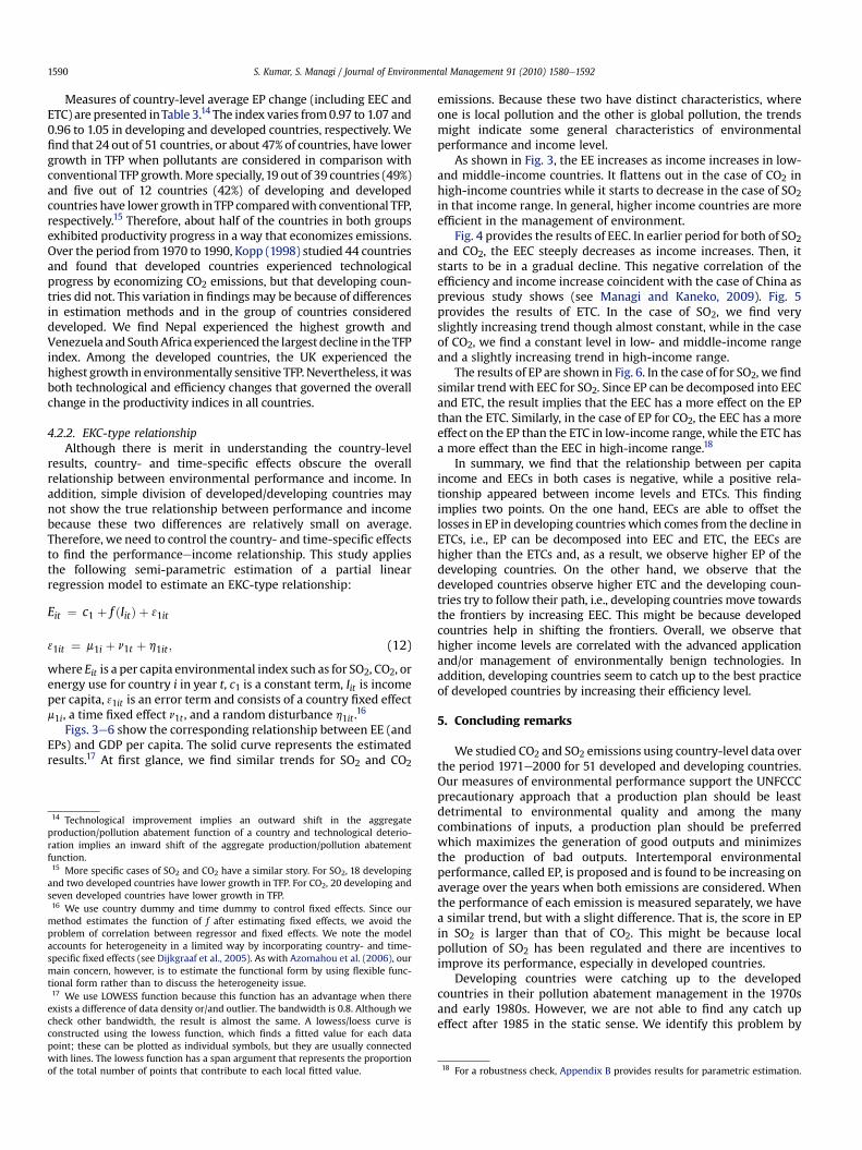
4.2.2. EKC-type relationshipAlthough there is merit in understanding the country-level

results, country- and time-specific effects obscure the overallrelationship between environmental performance and income. Inaddition, simple division of developed/developing countries maynot show the true relationship between performance and incomebecause these two differences are relatively small on average.Therefore, we need to control the country- and time-specific effectsto find the performanceeincome relationship. This study appliesthe following semi-parametric estimation of a partial linearregression model to estimate an EKC-type relationship:

Eit ¼ c1 þ f ðIitÞ þ 31it

31it ¼ m1i þ n1t þ h1it ; (12)

where Eit is a per capita environmental index such as for SO2, CO2, orenergy use for country i in year t, c1 is a constant term, Iit is incomeper capita, 31it is an error term and consists of a country fixed effectm1i, a time fixed effect n1t , and a random disturbance h1it .

16

Figs. 3e6 show the corresponding relationship between EE (andEPs) and GDP per capita. The solid curve represents the estimatedresults.17 At first glance, we find similar trends for SO2 and CO2

14 Technological improvement implies an outward shift in the aggregateproduction/pollution abatement function of a country and technological deterio-ration implies an inward shift of the aggregate production/pollution abatementfunction.15 More specific cases of SO2 and CO2 have a similar story. For SO2, 18 developingand two developed countries have lower growth in TFP. For CO2, 20 developing andseven developed countries have lower growth in TFP.16 We use country dummy and time dummy to control fixed effects. Since ourmethod estimates the function of f after estimating fixed effects, we avoid theproblem of correlation between regressor and fixed effects. We note the modelaccounts for heterogeneity in a limited way by incorporating country- and time-specific fixed effects (see Dijkgraaf et al., 2005). As with Azomahou et al. (2006), ourmain concern, however, is to estimate the functional form by using flexible func-tional form rather than to discuss the heterogeneity issue.17 We use LOWESS function because this function has an advantage when thereexists a difference of data density or/and outlier. The bandwidth is 0.8. Although wecheck other bandwidth, the result is almost the same. A lowess/loess curve isconstructed using the lowess function, which finds a fitted value for each datapoint; these can be plotted as individual symbols, but they are usually connectedwith lines. The lowess function has a span argument that represents the proportionof the total number of points that contribute to each local fitted value.

emissions. Because these two have distinct characteristics, whereone is local pollution and the other is global pollution, the trendsmight indicate some general characteristics of environmentalperformance and income level.

As shown in Fig. 3, the EE increases as income increases in low-and middle-income countries. It flattens out in the case of CO2 inhigh-income countries while it starts to decrease in the case of SO2in that income range. In general, higher income countries are moreefficient in the management of environment.

Fig. 4 provides the results of EEC. In earlier period for both of SO2and CO2, the EEC steeply decreases as income increases. Then, itstarts to be in a gradual decline. This negative correlation of theefficiency and income increase coincident with the case of China asprevious study shows (see Managi and Kaneko, 2009). Fig. 5provides the results of ETC. In the case of SO2, we find veryslightly increasing trend though almost constant, while in the caseof CO2, we find a constant level in low- and middle-income rangeand a slightly increasing trend in high-income range.

The results of EP are shown in Fig. 6. In the case of for SO2, we findsimilar trendwith EEC for SO2. Since EP can be decomposed into EECand ETC, the result implies that the EEC has a more effect on the EPthan the ETC. Similarly, in the case of EP for CO2, the EEC has a moreeffect on the EP than the ETC in low-income range, while the ETC hasa more effect than the EEC in high-income range.18

In summary, we find that the relationship between per capitaincome and EECs in both cases is negative, while a positive rela-tionship appeared between income levels and ETCs. This findingimplies two points. On the one hand, EECs are able to offset thelosses in EP in developing countries which comes from the decline inETCs, i.e., EP can be decomposed into EEC and ETC, the EECs arehigher than the ETCs and, as a result, we observe higher EP of thedeveloping countries. On the other hand, we observe that thedeveloped countries observe higher ETC and the developing coun-tries try to follow their path, i.e., developing countries move towardsthe frontiers by increasing EEC. This might be because developedcountries help in shifting the frontiers. Overall, we observe thathigher income levels are correlated with the advanced applicationand/or management of environmentally benign technologies. Inaddition, developing countries seem to catch up to the best practiceof developed countries by increasing their efficiency level.

5. Concluding remarks

We studied CO2 and SO2 emissions using country-level data overthe period 1971e2000 for 51 developed and developing countries.Our measures of environmental performance support the UNFCCCprecautionary approach that a production plan should be leastdetrimental to environmental quality and among the manycombinations of inputs, a production plan should be preferredwhich maximizes the generation of good outputs and minimizesthe production of bad outputs. Intertemporal environmentalperformance, called EP, is proposed and is found to be increasing onaverage over the years when both emissions are considered. Whenthe performance of each emission is measured separately, we havea similar trend, but with a slight difference. That is, the score in EPin SO2 is larger than that of CO2. This might be because localpollution of SO2 has been regulated and there are incentives toimprove its performance, especially in developed countries.

Developing countries were catching up to the developedcountries in their pollution abatement management in the 1970sand early 1980s. However, we are not able to find any catch upeffect after 1985 in the static sense. We identify this problem by

18 For a robustness check, Appendix B provides results for parametric estimation.


using semi-parametric estimation of the partial linear regressionmodel. This lack of a catch up effect may be explained by techno-logical progress being faster in developed countries. Once weconsider dynamic changes in efficiency as EP, we find a catch up ofthe low-income group to the high-income group. Our results arenot pessimistic because we observe the catch up of low-incomecountries. However, it is not optimistic either when comparingmiddle and high-income countries, because overall EP of both SO2and CO2 show developed countries improve much more thandeveloping countries. If these relationships continue in the future,it is hard to expect convergence in performances. Although ourstudy is different from traditional convergence studies and insteadwe examine the transformation of production processes by quan-tifying the opportunity cost of adopting alternative environmen-tally superior technologies, our results for CO2 appear to beconsistent with the study by Aldy (2007), which did not find CO2emissions convergence. We find the disconnection betweenincome convergence and emissions convergence (or EP conver-gence) suggesting caution about the design of emissions rightsallocated on a per capita basis. Our result suggests we must becareful to suggest any developed countries’ technological andmanagement assistances to developing countries and may needfurther efforts to increase their EE level apart from those associatedwith economic development.

Notwithstanding the striking features of the techniques usedhere, data limitations involved in estimation remains an importantfactor (Dowrick, 2005). The study is based on the assumption thatinputs and outputs variables used are of comparable quality andmeasured in the same manner across countries. It is, therefore,necessary to be cautious while applying these results to policypurposes.

Acknowledgments

The authors thank four anonymous referees for their helpfulcomments, and Tetsuya Tsurumi for his helpful assistance. Thisresearch was funded by the Ministry of Environment and a Grant-in-Aid for Scientific Research from the Japanese Ministry ofEducation, Culture, Sports, Science and Technology. The paper’scontent does not necessarily represent the views of these fundingagencies. Any errors remaining are the authors’ alone.

Appendix. Supplementary data

Supplementary data associated with this article can be found inthe online version, at doi:10.1016/j.jenvman.2010.03.003.

References

Aldy, J.E., 2007. Divergence in state-level per capita carbon dioxide emissions. LandEconomics 83 (3), 353e369.

Atkinson, S.E., Dorfman, R.H., 2005. Crediting electric utilities for reducing airpollution: Bayesian measurement of productivity and efficiency. Journal ofEconometrics 126, 445e468.

Azomahou, T., Laisney, F., Van, P.N., 2006. Economic development and CO2 emis-sions: a nonparametric panel approach. Journal of Public Economics 90 (6e7),1347e1363.

Ball, E., Färe, R., Grosskopf, S., Hernandez-Sancho, F., Nehring, R.F., 2002. Theenvironmental performance of the U.S. agricultural sector. In: Ball, V.E.,Norton, G.W. (Eds.), Agricultural Productivity: Measurement Sources of Growth.Kluwer Academic Publishers, pp. 257e275.

Chimeli, Ariaster B., Braden, John B., 2005. Total factor productivity and the envi-ronmental Kuznets curve. Journal of Environmental Economics and Manage-ment 49, 366e380.

Chung, Y., Färe, R., Grosskopf, S., 1997. Productivity and undesirable outputs:a directional distance function approach. Journal of Environmental Manage-ment 51, 229e240.

Cropper, M.L., Oates, W.E., 1992. Environmental economics: a survey. Journal ofEconomic Literature 30 (2), 675e740.

Dasgupta, S., Laplante, B., Wang, H., Wheeler, D., 2002. Confronting the environ-mental Kuznets curve. Journal of Economic Perspective 16 (1), 147e168.

Deacon, R.T., Norman, C.S., 2006. Does the environmental Kuznets curve describehow individual countries behave? Land Economics 82 (2), 291e315.

Dijkgraaf, E., Melenberg, B., Vollebergh, H.R.J., 2005. Environmental Kuznets Curvesfor CO2: Homogeneity vs. Heterogeneity. CentER Discussion Paper 2005.25.

Dinda, S., 2004. Environmental Kuznets curve hypothesis: a survey. EcologicalEconomics 49 (1), 431e455.

Dowrick, S., 2005. Errors in the Penn World Table demographic data. EconomicsLetters 87, 243e248.

Ebert, U., Welsch, H., 2007. Environmental emissions and production economics:implications of the materials balance. American Journal of AgriculturalEconomics 89 (2), 287e293.

Edgerton, M.D., 2009. Increasing crop productivity to meet global needs for feed,food, and fuel. Plant Physiology 149, 7e13.

Fairman, D., Ross, M., 1994. International Aid for the Environment: Lessons fromEconomic Development Assistance. Working Paper No. 94-4. The Center forInternational Affairs, Harvard University, Cambridge, MA.

Färe, R., Grosskopf, S., 2003. Nonparametric productivity analysis with undesirableoutputs: comment. American Journal of Agricultural Economics 85 (4),1070e1074.

Färe, R., Grosskopf, S., Noh, D.W., Weber, W., 2005. Characteristics of a pollutingtechnology: theory and practice. Journal of Econometrics 126, 469e492.

Färe, R., Grosskopf, S., Roos, P., 1995. Productivity and quality changes in Swedishpharmacies. International Journal of Production Economics 39, 137e144.

Färe, R., Grosskopf, S., Tyteca, D., 1996. An activity analysis model of the environ-mental performance of firms e application to fossil-fuel-fired electric utilities.Ecological Economics 18, 161e175.

Gollop, Frank M., Roberts, Mark J., 1983. Environmental regulations and produc-tivity growth: the case of fossil-fuelled electric power generation. Journal ofPolitical Economy, 654e674.

Grossman, G.M., Krueger, A.B., 1993. Environmental impacts of a North Americanfree trade agreement. In: Garber, P. (Ed.), The US Mexico Free Trade Agreement.MIT Press, Cambridge, MA, pp. 165e177.

Grossman, G.M., Krueger, A.B., 1995. Economic growth and the environment. TheQuarterly Journal of Economics 110, 353e377.

Hastie, T.J., Tibshirani, R.J., 1990. Generalized Additive Models. Chapman and Hall,New York.

Hailu, A., Veeman, T.S., 2001. Alternative methods for environmentally adjustedproductivity analysis. Agricultural Economics 25 (2e3), 211e218.

Heston, A., Summers, R., Aten, B., 2002. Penn Word Table 6.1. Mimeo, Center forInternational Comparisons, University of Pennsylvania.

Holtz-Eakin, D., Selden, T.M., 1995. Stoking the fires? CO2 emissions and economicgrowth. Journal of Public Economics 57, 85e101.

Jaffe, A.B., Newell, R.G., Stavins, R.N., 2003. Technological change and the environ-ment. In: Mäler, Karl-Göran, Vincent, Jeffrey (Eds.), Handbook of EnvironmentalEconomics. North-Holland, Elsevier Science, Amsterdam.

Kopp, Gary, 1998. Carbon dioxide emissions and economic growth: a structuralapproach. Journal of Applied Statistics 25 (4), 489e515.

Kortelainen, M., 2008. Dynamic environmental performance analysis: a Malmquistindex approach. Ecological Economics 64 (4), 701e715.

Kuosmanen, T., 2005. Weak disposability in nonparametric production analysis withundesirable outputs. American Journal of Agricultural Economics 87, 1077e1082.

Managi, S., 2004. Competitiveness and environmental policies for agriculture:testing the Porter hypothesis. International Journal of Agricultural Resources,Governance and Ecology 3 (3/4), 310e324.

Managi, S., 2006. Are there increasing returns to pollution abatement? Empiricalanalytics of the environmental Kuznets curve in pesticides. EcologicalEconomics 58 (3), 617e636.

Managi, S., Kaneko, S., 2009. Environmental performance and returns to pollutionabatement in China. Ecological Economics 68 (6), 1643e1651.

Managi, S., Opaluch, J.J., Jin, D., Grigalunas, T.A., 2005. Environmental regulationsand technological change in the offshore oil and gas industry. Land Economics81 (2), 303e319.

Marquetti, A., 2004. Extended Penn World Tables: Economic Growth Data on 118Countries. New School for Social Research.

Murty, M.N., Kumar, S., 2004. Environmental and Economic Accounting for Industry.Oxford University Press, New Delhi.

Pittman, R.W., 1981. Issues in pollution control: interplant cost differences andeconomies of scale. Land Economics 57 (1), 1e17.

Pittman, R.W., 1983. Multilateral productivity comparisons with undesirableoutputs. The Economic Journal 93, 883e891.

Prescott, E.C., 1998. Lawrence R. Klein lecture 1997 needed: a theory of total factorproductivity. International Economic Review 39 (3), 525e551.

Reinhard, S., Lovell, C.A.K., Thijssen, G., 1999. Econometric estimation of technicaland environmental efficiency: an application to Dutch dairy farms. AmericanJournal of Agricultural Economics 81 (1), 44e60.

Selden, T., Song, D., 1994. Environmental quality and development: is there a Kuz-nets curve for air pollution emissions? Journal of Environmental Economics andManagement 27, 147e162.

Schlenker, W., Hanemann, W.M., Fisher, A.C., 2006. The impact of global warmingon U.S. agriculture: an econometric analysis of optimal growing conditions.Review of Economics and Statistics 88 (1), 113e125.

Stern,D.I., 2005.Global sulfur emissions from1850 to2000.Chemosphere58,163e175.Stern, D.I., 2004. The rise and fall of the environmental Kuznets curve. World

Development 32, 1419e1439.

http://dx.doi.org/10.1016/j.jenvman.2010.03.003


Stern, D.I., 1998. Progress on the environmental Kuznets curve? Environment andDevelopment Economics 3, 173e196.

Taskin, F., Zaim, O., 2001. The role of international trade on environmental effi-ciency: a DEA approach. Economic Modelling 18, 1e17.

Verbeke, Tom, De Clercq, Marc, 2002. Environmental Quality and Economic Growth.Working Paper 2002/128, Department of Economics, University of Gent, Belgium.

Wossink, G.A.A., Oude Lansink, A.J.G.M., Struik, P.C., 2001. Non-separability andheterogeneity in integrated agronomiceeconomic analysis of nonpoint-sourcepollution. Ecological Economics 38, 345e357.

Yatchew, A., 2003. Semiparametric Regression for the Applied Econometrician.Cambridge University Press, Cambridge, UK.

Yoruk, B.K., Zaim, O., 2005. Productivity growth in OECD countries: a comparisonwithMalmquist productivity indexes. Journal of Comparative Economics 33, 401e420.

Zaim, O., Taskin, F., 2000. A Kuznets curve in environmental efficiency: an appli-cation on OECD countries. Environmental and Resource Economics 17, 21e36.

Zofio, J.L., Prieto, A.M., 2001. Environmental efficiency and regulatory standards: thecase of CO2 emissions from OECD countries. Resource and Energy Economics23, 63e83.

Documents

Environment and productivities in developed and developing countries: The case of carbon dioxide and sulfur dioxide