Envelopes andString Art

Gregory Quenell

1

0.2 0.4 0.6 0.8 1

0.2

0.4

0.6

0.8

1Activity:

Draw line segments connecting

(0, x) with (1− x, 0)

for x = 0.1, 0.2, . . . , 0.9.

Benefits:

• Gives you something to do during

calculus class

• Makes a pleasing pattern of inter-

secting lines

2

0.2 0.4 0.6 0.8 1

0.2

0.4

0.6

0.8

1Activity:

Draw line segments connecting

(0, x) with (1− x, 0)

for x = 0.1, 0.2, . . . , 0.9.

Benefits:

• Gives you something to do during

calculus class

• Makes a pleasing pattern of inter-

secting lines

• Provides an interesting curve to study

3

0.2 0.4 0.6 0.8 1

0.2

0.4

0.6

0.8

1Question:

What curve is this?

Observation:

The curve’s defining property is that

the sum of the x- and y-intercepts of

each of its tangent lines is 1.

That gives us the condition

y − xdy

dx+ x− y

dy/dx= 1

4

`୦

`β-

(0, α)

(0, β)

(1− β, 0) (1− α, 0)

Different approach:

For each α ∈ [0, 1], let `α be the line

segment connecting

(0, α) with (1− α, 0).

If α and β are close together, then the

intersection point of `α and `β is close

to a point on the curve.

Exercise:

For α 6= β, the segments `α and `β in-

tersect at the point

(αβ, (1− α)(1− β)).

5

`୦

`β-

Result:

As β → α, the point

(αβ, (1− α)(1− β))

approaches a point on the curve.

Thus, each point on the curve has the

form

limβ→α

(αβ, (1− α)(1− β))

for some α.

This is an easy limit, and we get the

parametrization

(α2, (1− α)2), 0 ≤ α ≤ 1

for our envelope curve.

6

0.2 0.4 0.6 0.8 1

0.2

0.4

0.6

0.8

1Remarks:

• The coordinates

x = α2 and y = (1− α)2

satisfy√

x +√

y = 1

so our curve is (one branch of) a

hypocircle with exponent 12.

• Stewart, p. 234, problem 8 says

“Show that the sum of the x- and y-intercepts of any tangent line to

the curve√

x +√

y =√

c is equal to c.”

7

1 2

1

2

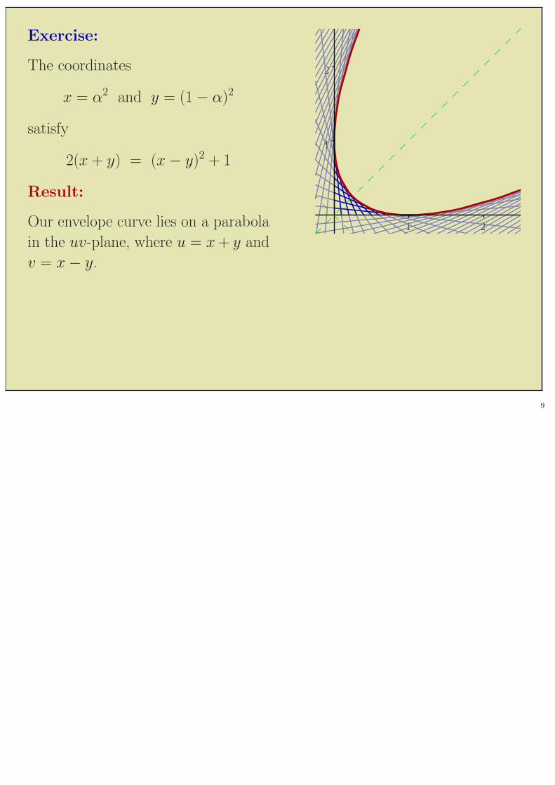
Exercise:

The coordinates

x = α2 and y = (1− α)2

satisfy

2(x + y) = (x− y)2 + 1

Result:

Our envelope curve lies on a parabola

in the uv-plane, where u = x + y and

v = x− y.

8

1 2

1

2

Exercise:

The coordinates

x = α2 and y = (1− α)2

satisfy

2(x + y) = (x− y)2 + 1

Result:

Our envelope curve lies on a parabola

in the uv-plane, where u = x + y and

v = x− y.

9

Activity: String Art

Drive nails at equal intervals

along two lines, and connect

the nails with decorative string.

10

Activity: String Art

The envelope curves are the images, under a linear transformation, of

parabolas tangent to the coordinate axes. That is, they are parabolas

tangent to the nailing lines.

11

Colin

IIA IIB

RoseIA

IB

(2, 0)

(4, 2)

(3, 6)

(0, 0)

Digression: Game Theory

Consider a two-person, non-zero-sum

game in which each player has two

strategies.

Pay

offto

Col

in

Payoff to Rose

(IB,IIB) (IA,IIA)

(IB,IIA)

(IA,IIB)

2

4

6

2 4

Such a game has four possible payoffs.

We list them in a payoff matrix.

We can show the payoffs to Rose and

Colin as points in the payoff plane.

12

Colin

IIA IIB

RoseIA

IB

(2, 0)

(4, 2)

(3, 6)

(0, 0)

Assumptions:

We assume each player adopts a

mixed strategy:

• Rose plays IA with probability p

and IB with probability 1− p.

• Colin plays IIA with probability

q and IIB with probability 1− q

The expected payoff is then

pq(2, 0) + p(1− q)(3, 6) + (1− p)q(4, 2) + (1− p)(1− q)(0, 0)

orp [q(2, 0) + (1− q)(3, 6)] + (1− p) [q(4, 2) + (1− q)(0, 0)]

orq [p(2, 0) + (1− p)(4, 2)] + (1− q) [p(3, 6) + (1− p)(0, 0)]

13

Pay

offto

Col

in

Payoff to Rose

(IB,IIB) (IA,IIA)

(IB,IIA)

(IA,IIB)

2

4

6

4

Possible payoff points:

Each value of q determines one point

on the line from (2, 0) to (3, 6) and

one point on the line from (4, 2) to

(0, 0).

Then p is the parameter for a line

segment between these points.

p [q(2, 0) + (1− q)(3, 6)]

+(1− p) [q(4, 2) + (1− q)(0, 0)]

14

Pay

offto

Col

in

Payoff to Rose

(IB,IIB) (IA,IIA)

(IB,IIA)

(IA,IIB)

2

4

6

4

Possible payoff points:

Alternatively, each value of p

determines one point on the line from

(2, 0) to (4, 2) and one point on the

line from (3, 6) to (0, 0).

Then q is the parameter for a line

segment between these points.

q [p(2, 0) + (1− p)(4, 2)]

+(1− q) [p(3, 6) + (1− p)(0, 0)]

15

Pay

offto

Col

in

Payoff to Rose

(IB,IIB) (IA,IIA)

(IB,IIA)

(IA,IIB)

2

4

6

4

Possible payoff points:

Either way, the expected payoff is

contained in a region bounded by

four lines and a parabolic envelope

curve.

If the game is played a large number of

times and the average payoff converges

to a point outside this region, then the

players’ randomizing devices are not

independent.

This could be due to collusion, espionage, or maybe just poor

random-number generators.

16

(0, Y (α))

(0, Y (β))

(X(α), 0) (X(β), 0)

Generalization:

Unequal Spacing

Draw line segments `α connecting

(X(α), 0) with (0, Y (α))

for arbitrary differentiable functions

X and Y .

These are “spacing functions”.

Exercise:

Segments `α and `β intersect at the point

(X(α)X(β)(Y (β)− Y (α))

X(α)Y (β)− Y (α)X(β),Y (α)Y (β)(X(α)−X(β))

X(α)Y (β)− Y (α)X(β)

)

17

(0, Y (α))

(X(α), 0)

Generalization:

Unequal Spacing

To find a point on the envelope

curve, we need to compute

limβ→α

(X(α)X(β)(Y (β)− Y (α))

X(α)Y (β)− Y (α)X(β),Y (α)Y (β)(X(α)−X(β))

X(α)Y (β)− Y (α)X(β)

)

18

Calculation:

“Plugging in” α for β gives

(X(α)X(α)(Y (α)− Y (α))

X(α)Y (α)− Y (α)X(α),Y (α)Y (α)(X(α)−X(α))

X(α)Y (α)− Y (α)X(α)

)

=

(0

0,0

0

)

So we try something else . . .

The x-coordinate of a point on the envelope is

limβ→α

X(α)X(β)(Y (β)− Y (α))

X(α)Y (β)− Y (α)X(β)

19

Calculation: limβ→α

X(α)X(β)(Y (β)− Y (α))

X(α)Y (β)− Y (α)X(β)

= limβ→α

X(α)X(β)(Y (β)− Y (α))

X(α)Y (β)−X(α)Y (α) + X(α)Y (α)− Y (α)X(β)

= limβ→α

X(α)X(β)(Y (β)− Y (α))

X(α)(Y (β)− Y (α))− Y (α)(X(β)−X(α))

= limβ→α

X(α)X(β)( Y (β)−Y (α)β−α )

X(α)( Y (β)−Y (α)β−α )− Y (α)( X(β)−X(α)

β−α )

=X(α)X(α) · lim

β→α

Y (β)−Y (α)β−α

X(α) · limβ→α

Y (β)−Y (α)β−α − Y (α) · lim

β→α

X(β)−X(α)β−α

=(X(α))2Y ′(α)

X(α)Y ′(α)− Y (α)X ′(α)

20

Result:

Do the same thing for the

y-coordinate

limβ→α

Y (α)Y (β)(X(α)−X(β))

X(α)Y (β)− Y (α)X(β)

=−(Y (α))2X ′(α)

X(α)Y ′(α)− Y (α)X ′(α)

We get the parametrization

((X(α))2Y ′(α)

X(α)Y ′(α)− Y (α)X ′(α),

−(Y (α))2X ′(α)

X(α)Y ′(α)− Y (α)X ′(α)

)

for the envelope curve.

21

Example:

The picture shows lines generated by

X(α) = 4

(α− 1

2

)3

+1

2

along the x-axis and

Y (α) = 1− α2

along the y-axis.

The formula from the previous slide gives the parametrization

(− 2α3(4α2 − 6α + 3)

4α4 − 15α2 + 12α− 3,− 3(2α− 1)2(α2 − 1)2

4α4 − 15α2 + 12α− 3

)

for the envelope curve.

22

Y (α)

︸ ︷︷ ︸X(α)

Example:

A ladder of length L slides down a

wall.

What is the envelope curve?

Solution:

We want (X(α))2 + (Y (α))2 = L2,

so we may as well take

X(α) = L sin(α) and Y (α) = L cos(α).

23

Y (α)

︸ ︷︷ ︸X(α)

Example:

A ladder of length L slides down a

wall.

What is the envelope curve?

Solution:

We want (X(α))2 + (Y (α))2 = L2,

so we may as well take

X(α) = L sin(α) and Y (α) = L cos(α).

We get(

(X(α))2Y ′(α)

X(α)Y ′(α)− Y (α)X ′(α),

−(Y (α))2X ′(α)

X(α)Y ′(α)− Y (α)X ′(α)

)

= (L sin3(α), L cos3(α))

24

Y (α)

︸ ︷︷ ︸X(α)

Remarks:

The envelope curve, parametrized by

x = L sin3(α) and y = L cos3(α)

has equation

x23 + y

23 = L

23

(This is called an astroid.)

25

¾ -

6

?

x

y

Remarks:

The envelope curve, parametrized by

x = L sin3(α) and y = L cos3(α)

has equation

x23 + y

23 = L

23

(This is called an astroid.)

So if you want to carry your ladder around a corner from a hallway of

width x into a hallway of width y, the length of the ladder has to satisfy

L23 ≤ x

23 + y

23

26

Further Generalization:

Instead of using the axes as nailing

lines, use parametrized curves

(X1(α), Y1(α)) and (X2(α), Y2(α))

Exercise:

Find the intersection point of `α and

`β, and show that as β → α, this

point approaches

x =(X1X

′2 −X ′

1X2)(Y2 − Y1)− (X1Y′2 − Y ′

1X2)(X2 −X1)

(X ′2 −X ′

1)(Y2 − Y1)− (Y ′2 − Y ′

1)(X2 −X1)

y =(Y1X

′2 −X ′

1Y2)(Y2 − Y1)− (Y1Y′2 − Y ′

1Y2)(X2 −X1)

(X ′2 −X ′

1)(Y2 − Y1)− (Y ′2 − Y ′

1)(X2 −X1)

27

Example:

Let

X1(α) = cos(α)

Y1(α) = sin(α)

X2(α) = cos(2α)

Y2(α) = sin(2α)

Interpretations:

• Drive nails around a circle at regular intervals. Connect nail 1 to nail 2,

2 to 4, 3 to 6, 4 to 8, 5 to 10, and so on.

• (Simoson, 2000) Two runners set off around a circular track with a

bungee cord stretched between them. The second runner goes twice as

fast as the first.

28

Yet Another Exercise:

Substitute

X1(α) = cos(α)

Y1(α) = sin(α)

X2(α) = cos(2α)

Y2(α) = sin(2α)

into

x =(X1X

′2 −X ′

1X2)(Y2 − Y1)− (X1Y′2 − Y ′

1X2)(X2 −X1)

(X ′2 −X ′

1)(Y2 − Y1)− (Y ′2 − Y ′

1)(X2 −X1)

y =(Y1X

′2 −X ′

1Y2)(Y2 − Y1)− (Y1Y′2 − Y ′

1Y2)(X2 −X1)

(X ′2 −X ′

1)(Y2 − Y1)− (Y ′2 − Y ′

1)(X2 −X1)

and simplify.

29

Answer:

x =cos 2α + 2 cos α

3

y =sin 2α + 2 sin α

3

30

Answer:

x =cos 2α + 2 cos α

3

y =sin 2α + 2 sin α

3

31

Answer:

x =cos 2α + 2 cos α

3

y =sin 2α + 2 sin α

3

Write this as

x =2

3cos α +

1

3cos 2α, y =

2

3sin α +

1

3sin 2α

to see that our curve is an epicycloid, traced by a point on a circle of radius13 rolling around the outside of a fixed circle of radius 1

3.

32

1 2

1

2

Conclusion:

The parabola, the astroid, and the

epicycloid are all easy string-art

curves.

Some other easy ones are the

hyperbola and the circle.

33

References:

• Edouard Goursat, A Course in Mathematical Analysis, Dover, 1959,

Volume I, Chapter X.

• GQ, Envelopes and String Art, to appear in Mathematics Magazine.

• Andrew J. Simoson, The trochoid as a tack in a bungee cord,

Mathematics Magazine 73(3), 2000.

• Philip D. Straffin, Game Theory and Strategy, MAA, 1993.

• David H. Von Seggern, CRC Standard Curves and Surfaces, CRC

Press, 1993.

34