Embed Size (px)
Citation preview

Enumeration in Algebra and Geometry
by
Alexander Postnikov
Master of Science in MathematicsMoscow State University, 1993
Submitted to the Department of Mathematicsin partial fulfillment of the requirements for the degree of
Doctor of Philosophy in Mathematics
at the
MASSACHUSETTS INSTITUTE OF TECHNOLOGY
June 1997
c© Massachusetts Institute of Technology 1997. All rights reserved.
Author . . . . . . . . . . . . . . . . . . . . . . . . . . . . . . . . . . . . . . . . . . . . . . . . . . . . . . . . . . . . . .Department of Mathematics
May 2, 1997
Certified by. . . . . . . . . . . . . . . . . . . . . . . . . . . . . . . . . . . . . . . . . . . . . . . . . . . . . . . . . .Richard P. Stanley
Professor of Applied MathematicsThesis Supervisor
Accepted by . . . . . . . . . . . . . . . . . . . . . . . . . . . . . . . . . . . . . . . . . . . . . . . . . . . . . . . . .Hung Cheng
Chairman, Applied Mathematics Committee
Accepted by . . . . . . . . . . . . . . . . . . . . . . . . . . . . . . . . . . . . . . . . . . . . . . . . . . . . . . . . .Richard Melrose
Chair, Department Committee on Graduate Students

Enumeration in Algebra and Geometryby
Alexander Postnikov
Submitted to the Department of Mathematicson May 2, 1997, in partial fulfillment of the
requirements for the degree ofDoctor of Philosophy in Mathematics
Abstract
This thesis is devoted to solution of two classes of enumerative problems.The first class is related to enumeration of regions of hyperplane arrangements.
We investigate deformations of Coxeter arrangements. In particular, we prove a con-jecture of Stanley on the numbers of regions of Linial arrangements. These numbershave several additional combinatorial interpretations in terms of trees, partially or-dered sets, and tournaments. We study a more general class of truncated affinearrangements, counting their regions, giving formulas for their Poincare polynomials,and proving a “Riemann hypothesis” on location of zeros of the latter. In addition,we find a couple of new interpretations for the Catalan numbers.
The second class of problems comes from enumerative algebraic geometry andSchubert calculus and is related to Gromov-Witten invariants of complex flag man-ifolds. We present a method for their calculation using a new construction for thequantum cohomology ring of the flag manifold. This construction provides quantumanalogues of results of Bernstein, Gelfand, and Gelfand on this subject and of thetheory of Schubert polynomials of Lascoux and Schutzenberger. The quantum versionof Monk’s formula is established, and a general Pieri-type formula is derived.
While being remote from each other at first glance, both these subjects can beattacked with algebraic and combinatorial methods.
Thesis Supervisor: Richard P. StanleyTitle: Professor of Applied Mathematics

Acknowledgments
First of all, I thank my parents.I am greatly indebted to my advisor Richard Stanley. His book Enumerative
Combinatorics, vol. 1, deeply influenced me long before I had the privilege of meetingProfessor Stanley personally.
My initial interest in mathematics was mainly the result of efforts of my highschool teacher Sergey Grigorievich Roman, to whom my thanks are due.
I benefited greatly from a unique opportunity to attend the seminar of IsraelGelfand in Moscow. I wish to express my gratitude to him as well as to Askold Kho-vanskii, Vladimir Retakh, Andrei Zelevinsky, and many other people who contributedto the unforgettable mathematical environment.
I am grateful to Sergey Fomin and to Bertram Kostant. My warm regards aredue to Gian-Carlo Rota. Communication with them was helpful and enriching.
I would also like to thank, possibly repeating names, my coauthors: Sergey Fomin,Israel Gelfand, Sergei Gelfand, Mark Graev, and Richard Stanley.
My thanks are due to Alexander Astashkevich, Arkady Berenstein, and OlegGleizer for helpful discussions related and not related to mathematics.
At last, I thank again the people who agreed to be the members of my thesiscommittee: Sergey Fomin, Richard Stanley, and Andrei Zelevinsky.
3

4

Contents
1 Hyperplane Arrangements 91.1 Introduction . . . . . . . . . . . . . . . . . . . . . . . . . . . . . . . . 91.2 Arrangements of Hyperplanes . . . . . . . . . . . . . . . . . . . . . . 12
1.2.1 Regions and Poincare polynomials . . . . . . . . . . . . . . . . 121.2.2 Coxeter arrangements . . . . . . . . . . . . . . . . . . . . . . 131.2.3 Whitney’s formula . . . . . . . . . . . . . . . . . . . . . . . . 141.2.4 Deformations of Coxeter arrangements . . . . . . . . . . . . . 161.2.5 The Orlik-Solomon algebra . . . . . . . . . . . . . . . . . . . . 18
1.3 Catalan Miscellanea . . . . . . . . . . . . . . . . . . . . . . . . . . . . 191.3.1 Semiorders . . . . . . . . . . . . . . . . . . . . . . . . . . . . . 191.3.2 Reciprocity for hyperplane arrangements . . . . . . . . . . . . 211.3.3 Polyhedra and their triangulations . . . . . . . . . . . . . . . 23
1.4 Alternating Trees and the Linial Arrangement . . . . . . . . . . . . . 251.4.1 Counting alternating trees . . . . . . . . . . . . . . . . . . . . 251.4.2 Local binary search trees . . . . . . . . . . . . . . . . . . . . . 271.4.3 On stability and fickleness . . . . . . . . . . . . . . . . . . . . 281.4.4 The Linial arrangement . . . . . . . . . . . . . . . . . . . . . 291.4.5 Balanced graphs . . . . . . . . . . . . . . . . . . . . . . . . . 301.4.6 Sleek posets and semiacyclic tournaments . . . . . . . . . . . 31
1.5 Truncated Affine Arrangements . . . . . . . . . . . . . . . . . . . . . 341.5.1 Functional equations . . . . . . . . . . . . . . . . . . . . . . . 341.5.2 Formulae for the characteristic polynomial . . . . . . . . . . . 381.5.3 Roots of the characteristic polynomial . . . . . . . . . . . . . 40
1.6 Asymptotics and Random Trees . . . . . . . . . . . . . . . . . . . . . 411.6.1 Characteristic polynomials and trees . . . . . . . . . . . . . . 411.6.2 Random trees . . . . . . . . . . . . . . . . . . . . . . . . . . . 421.6.3 Asymptotics of characteristic polynomials . . . . . . . . . . . 45
2 Quantum Cohomology of Flag Manifolds 492.1 Introduction . . . . . . . . . . . . . . . . . . . . . . . . . . . . . . . . 492.2 Background . . . . . . . . . . . . . . . . . . . . . . . . . . . . . . . . 54
2.2.1 Flag manifold and Schubert cells . . . . . . . . . . . . . . . . 542.2.2 NilHecke ring and Schubert polynomials . . . . . . . . . . . . 552.2.3 Quantum cohomology and Gromov-Witten invariants . . . . . 57
2.3 Combinatorial Quantum Multiplication . . . . . . . . . . . . . . . . . 59
5
2.3.1 Commuting elements in the nilHecke ring . . . . . . . . . . . . 592.3.2 Combinatorial quantization . . . . . . . . . . . . . . . . . . . 61
2.4 Standard Elementary Polynomials . . . . . . . . . . . . . . . . . . . . 632.4.1 Straightening . . . . . . . . . . . . . . . . . . . . . . . . . . . 632.4.2 Deformation . . . . . . . . . . . . . . . . . . . . . . . . . . . . 652.4.3 Straightforward deformation . . . . . . . . . . . . . . . . . . . 69
2.5 Quantum Schubert Polynomials . . . . . . . . . . . . . . . . . . . . . 702.5.1 Simple properties . . . . . . . . . . . . . . . . . . . . . . . . . 702.5.2 Orthogonality property . . . . . . . . . . . . . . . . . . . . . . 722.5.3 Axiomatic characterization . . . . . . . . . . . . . . . . . . . . 74
2.6 Monk’s Formula and its Extensions . . . . . . . . . . . . . . . . . . . 762.6.1 Quantum version of Monk’s formula . . . . . . . . . . . . . . . 762.6.2 Quadratic ring . . . . . . . . . . . . . . . . . . . . . . . . . . 772.6.3 General version of Pieri’s formula . . . . . . . . . . . . . . . . 782.6.4 Action on the quantum cohomology . . . . . . . . . . . . . . . 802.6.5 Proof of general Pieri’s formula . . . . . . . . . . . . . . . . . 82
6

What is this thesis about?
Enumerative problems come up in various areas of mathematical research. Some ofthem can be formulated in purely combinatorial terms, while for others even such aformulation can be the sole purpose of a highly nontrivial investigation.
In this thesis,1 I concern with several problems that appear in two different fieldsof mathematics.
The first topic is related to the classical question: “On how many pieces a certaincollection of hyperplanes subdivides a linear space?” It is usually not hard to answerthis question for a generic collection of hyperplanes. But for some special hyperplanearrangements the answer can be much more interesting than for the generic case, andyet not so easy to gain.
The second task of this thesis belongs to the area of enumerative geometry andis similar to the (no less classical) question: “How many algebraic curves of a givendegree pass through a given set of points, assuming that the conditions imply thatthis number is finite?” This, usually hard, question can sometimes be solved with thehelp of recently discovered algebraic structures.
Although our two aims seem to be far from each other, our means are close. Theseare the methods of algebraic combinatorics.
Two parts of the thesis are independent from each other and, consequently, thereader may peruse them in whatever order he or she prefers. A person more inclinedto read about Schubert calculus and quantum cohomology may skip the first part anddirectly proceed to reading the second part. On the other hand, a person more atease with hyperplane arrangements and combinatorics of trees and posets may chooseto ignore the second part and concentrate entirely on the first part of the thesis.
When determined on which part to start with, the reader should first acquainthimself or herself with the corresponding introduction, afterwards keep on readingthe remaining sections.
1The thesis contains the results obtained in the papers [17, 20, 42, 43, 44] written in collaborationwith coauthors and without at various time during my graduate studies at M.I.T.
7

8

Chapter 1
Hyperplane Arrangements
This part of my thesis is based on a joint work with Richard Stanley [44]. It alsocontains the results of [42] as well as some results of [20] obtained in collaborationwith Israel Gelfand and Mark Graev.
1.1 Introduction
The main objects in this chapter are arrangements of hyperplanes. The simplestinvariant of a hyperplane arrangement A in a real vector space is its number ofregions r(A), i.e., the number of connected components, on which hyperplanes sub-divide the space. Another invariant is the cohomology ring of the complement to thecomplexification of A. It can be shown that the dimension of the cohomology ring isequal to r(A).
The Coxeter arrangement of type An−1 is the arrangement of hyperplanes
xi − xj = 0, 1 ≤ i < j ≤ n. (1.1.1)
The regions of this arrangement, n! in number, correspond different ways of orderingthe sequence x1, . . . , xn . The cohomology ring of the complement was calculatedby Arnold [1]. In particular, he showed that its Poincare polynomial, which is thegenerating function for the Betti numbers, is equal to (1+q) (1+2q) · · · (1+(n−1)q).
In this chapter we study a more general class of arrangements which can be viewedas deformations of the arrangement (1.1.1). One of them is the Linial arrangement Ln
given by
xi − xj = 1, 1 ≤ i < j ≤ n. (1.1.2)
A tree on the vertices labelled by integers is called alternating if the labels alongevery path alternate, i.e., form an up-down or down-up sequence. Our main result onLinial arrangements says that the number of regions of the arrangement Ln is equalto the number of alternating trees on the vertices 1, . . . , n+ 1.
The arrangement Ln was first considered by Linial and Ravid. They calculatedthe numbers of regions of Ln for several first values of n. The statement above
9

was conjectured by Stanley on the base of their numerical results. Alternating treesearlier appeared in [20] in the context of a certain hypergeometric system and arelated polyhedron, then they were studied in [42]. The formula for the number ofalternating trees, proved in [42], thus provides the one for the number of regions ofthe Linial arrangements. Explicitly,
r(Ln) = 2−n
n∑k=1
(n
k
)(k + 1)n−1 .
In addition, these numbers have several other combinatorial interpretations. Forexample, we show that r(Ln) is also equal to the number of binary trees on thevertices 1, . . . , n such that left children are always less than their parents and rightchildren are always bigger.
We study a more general class of arrangements called truncated affine arrange-ments. They are finite subarrangements of the affine type An−1 hyperplane arrange-ment, and explicitly given by the following equations, where a and b are fixed integers,
xi − xj = k, 1 ≤ i < j ≤ n,−a < k < b . (1.1.3)
For instance, the Linial arrangement Ln corresponds to the case of a = 0 and b = 2.
Remind that the characteristic polynomial of a hyperplane arrangement is relatedto the Poincare polynomial by a simple transformation. For 0 ≤ a < b, we provethat the characteristic polynomial χab
n (q) of the truncated affine arrangement (1.1.3)equals
χabn (q) = (b− a)−1(Sa + Sa+1 + · · ·+ Sb−1)n · qn−1 ,
where S is the shift operator S : f(q) 7→ f(q − 1).
As a byproduct of this statement, a “Riemann hypothesis” on zeros of the charac-teristic polynomial is obtained. Namely, we demonstrate that if a 6= b then all rootsof the characteristic polynomial χab
n (q) have the same real part equal to (a+b−1)n/2.In contrast, for a = b, the roots are real. If a = b− 1 then all roots are equal to na.
An asymptotics of characteristic polynomials of Linial arrangements is found. Inparticular, for “big” n, the distance between two adjacent roots of the characteristicpolynomial is “close” to πα , where α = 1.199678 . . . is the root of the equation
e2α = (α+ 1)(α− 1)−1, α > 1 .
We also investigate some arrangements related to the Catalan numbers, and provea reciprocity result for certain deformations of Coxeter arrangements with and withoutcentral hyperplanes (1.1.1). In addition, we present several interpretations of theCatalan numbers.
In the rest of Introduction we outline how this chapter is organized. Section 1.2 isdevoted to main definitions and general theorems from the theory of hyperplane ar-rangements. We discuss regions, Poincare and characteristic polynomials, intersectionposet, and Orlik-Solomon algebra. In Section 1.2.3 we review several general theo-
10

rems on hyperplane arrangements, including a variant of the NBC Theorem, which isour main technical tool. Then in Section 1.2.4 we apply this theorem to deformationsof Coxeter arrangements.
In Section 1.3 we study the hyperplane arrangements related, in a special case,to interval orders and the Catalan numbers. In Section 1.3.2 we prove a generalreciprocity result for such arrangements. We also mention several new interpretationsof the Catalan numbers.
A discussion of alternating trees, Linial arrangements, and other related objectsis the purpose of Section 1.4. We give the main result on Linial arrangements andalternating trees (Theorem 1.4.5), and introduce several combinatorial objects whosenumbers are equal to the number of regions of the Linial arrangement: local binarysearch trees, sleek posets, semiacyclic tournaments, FIS and SIF trees. In Section 1.4.6we prove a theorem on characterization of sleek posets in terms of forbidden subposets.
In Section 1.5 we study truncated affine arrangements. We provide a proof to theresult on numbers of regions of these arrangements and their characteristic polyno-mials (Theorem 1.5.7). To do that, we first establish in Section 1.5.1 a functionalequation for the exponential generating function of the numbers of regions. Then wededuce a “Riemann hypothesis.”
In Section 1.6 we study “random” trees and asymptotics of characteristic polyno-mials.
11

1.2 Arrangements of Hyperplanes
In this section we give main definitions and several general theorems from the theoryof hyperplane arrangements. For more details, see [61, 38, 39]. We prove a generalizedWhitney’s theorem and its corollary—the NBC theorem. Then we apply them forcalculation of the numbers of regions and the Poincare polynomials of deformationsof type A Coxeter arrangements. Finally, we recall the construction of the Orlik-Solomon algebra.
1.2.1 Regions and Poincare polynomials
An arrangement of hyperplanes or hyperplane arrangement is a discrete collection ofaffine hyperplanes in a vector space. Let A be a finite arrangement of hyperplanes ina real vector space V . We will always assume1 that the vectors dual to hyperplanes inA span the space V ∗ and call A a nondegenerate arrangement in this case. A regionof A is a connected component of the complement to hyperplanes in the arrangement.Let r(A) denote the number of regions of A.
The Poincare polynomial is a q-analogue for these numbers. Let AC denote thecomplexified arrangement A, that is the collection of the hyperplanes H⊗C, H ∈ A,in the complex vector space V ⊗C. A let CA be the complement to hyperplanes of ACin V ⊗C. The Poincare polynomial PoinA(q) of A is the generating function for theBetti numbers of CA:
PoinA(q) =∑k≥0
dim Hk(CA,C) qk.
The intersection poset2 LA of the arrangement A is the collection of all nonemptyintersections of hyperplanes in A ordered by reverse inclusion. Thus the poset LAhas a unique minimal element3 0 = V . The characteristic polynomial of A is thendefined by
χA(q) =∑z∈LA
µ(0, z) qdim z, (1.2.1)
where µ denotes the Mobius function of LA (see [51, Section 3.7]). The generalproperties of geometric lattices [51, Proposition 3.10.1] imply, for example, that thesign of µ(0, z) is equal to (−1)codim z.
The following fundamental result of Orlik and Solomon [38] establishes a relationbetween the Poincare and characteristic polynomials and the number of regions r(A)as well as the number of bounded regions of A.
1without loss of generality2Here and elsewhere the word “poset” stands for “partially ordered set.”3This poset has a unique maximal element if and only if the intersections of hyperplanes in A is
nonempty. In this case LA is a geometric lattice.
12

Theorem 1.2.1 Assume that A is a nondegenerate arrangement in an l-dimensionalvector space. Then
χA(q) = ql PoinA(−q−1). (1.2.2)
The dimension of the cohomology ring dim H∗(CA,C) = PoinA(1) = (−1)lχA(−1) isthe number of regions r(A) of A. Likewise, the alternating sum of the Betti numbersPoinA(−1) = χA(1) is the number of bounded regions of A.
A combinatorial proof the last two statements of this theorem in terms of thecharacteristic polynomial was earlier given by T. Zaslavsky in [61].
1.2.2 Coxeter arrangements
Let V be a real l-dimensional vector space, and let Φ be a root system in V ∗ witha distinguished set of positive roots Φ+ = φ1, φ2, . . . , φN (see [8, Ch. VI]). TheCoxeter arrangement A(Φ) is the arrangement of hyperplanes in V given by
φi(x) = 0, 1 ≤ i ≤ N, (1.2.3)
where x ∈ V .
The number of regions (Weyl chambers) of A(Φ) is equal to the order of thecorresponding Weyl group W .
AA
AA
AA
AA
AA
r
Figure 1-1: The Coxeter hyperplane arrangement A3.
In the case of a type A root system it is more convenient to use the augmentedindex n = l + 1. Let Vn denote the subspace (hyperplane) of all vectors (x1, . . . , xn)in Rn such that x1 + · · · + xn = 0. The Coxeter arrangement4 An = A(An−1) is thearrangement of hyperplanes in Vn explicitly given by
xi − xj = 0, 1 ≤ i < j ≤ n. (1.2.4)
4or Braid arrangement
13

To compute the number of regions of this arrangement is not much harder than tocompute the order of the symmetric group Sn—both these numbers are n! . Arnold [1]calculated the cohomology ring H∗(CAn ,C) (see Corollary 1.2.14). In particular, hedemonstrated that the characteristic polynomial of An is equal to
χAn(q) = (q − 1)(q − 2) · · · (q − n+ 1) . (1.2.5)
Brieskorn [9] generalized Arnold’s result to the case of any Coxeter arrange-ment. His formula for the characteristic polynomial of (1.2.3) involves the exponentsm1, . . . ,ml of the corresponding Weyl group W :
χA(Φ)(q) = (q −m1)(q −m2) · · · (q −ml) .
1.2.3 Whitney’s formula
In this section we prove several essentially well-known results on hyperplane arrange-ments that will be useful in the sequel.
Consider the arrangement A of hyperplanes in V ∼= Rl given by equations
hi(x) = ai, 1 ≤ i ≤ N, (1.2.6)
where x ∈ V , the hi ∈ V ∗ are linear functionals on V , and the ai are real numbers.
We call a subset I in 1, 2, . . . , N central if the intersection of the hyperplaneshi(x) = ai, i ∈ I, is nonempty. For a subset I = i1, i2, . . . , im, denote by rk(I) thedimension (rank) of the linear span of the vectors hi1 , . . . , him .
The following statement is a generalization of a classical Whitney’s formula [57].
Theorem 1.2.2 [44, Theorem 4.1] The Poincare and characteristic polynomials ofthe arrangement A are equal to
PoinA(q) =∑
I
(−1)|I|−rk(I) qrk(I), (1.2.7)
χA(q) =∑
I
(−1)|I| ql−rk(I), (1.2.8)
where I ranges over all central subsets in 1, 2, . . . , N. In particular, the number ofregions of A is equal to
r(A) =∑
I
(−1)|I|−rk(I),
and the number of bounded regions is equal to∑I
(−1)|I|.
We need the well-known cross-cut theorem.
14

Lemma 1.2.3 [51, Corollary 3.9.4] Let L be a finite lattice with the minimal ele-ment 0 and the maximal element 1, and let X be a subset of vertices in L such that(a) 0 6∈ X, and (b) if y ∈ L, y 6= 0 then x ≤ y for some x ∈ X (such elements arecalled atoms). Then
µL(0, 1) =∑
k
(−1)k nk, (1.2.9)
where nk is the number of k-element subsets in X with join equal to 1.
Now we can easily deduce Theorem 1.2.2.
Proof — Let z be any element in the intersection poset LA, and let L(z) be thesubposet of all elements x ∈ LA such that x ≤ z, i.e., the subspace x contains z. Infact, L(z) is a geometric lattice. Let X be the set of all hyperplanes from A whichcontain z. If we apply Lemma 1.2.3 to L = L(z) and sum (1.2.9) over all z ∈ LA, weget the formula (1.2.8). Then, by (1.2.2), we get (1.2.7).
A circuit is a minimal subset I such that rk(I) = |I|− 1. In other words, a subsetI = i1, i2, . . . , im is a circuit if there exists a nonzero vector (λ1, λ2, . . . , λm), uniqueup to a nonzero factor, such that λ1hi1 + λ2hi2 + · · · + λmhim = 0. It is not difficultto see that a circuit I is central if, in addition, we have λ1ai1 +λ2ai2 + · · ·+λlail = 0.Thus, if a1 = · · · = aN = 0 then all circuits are central, and if the ai are generic thenthere are no central circuits.
A subset I is called acyclic if |I| = rk(I), i.e., I contains no circuits. It is clearthat any acyclic subset is central.
Corollary 1.2.4 In the case when the ai are generic, the Poincare polynomial equals
PoinA(q) =∑
I
q|I|,
where the sum is over all acyclic subsets I in 1, 2, . . . , N. In particular, the numberof regions r(A) is equal to the number of acyclic subsets.
Indeed, in this case a subset I is acyclic if and only if it is central.
Remark 1.2.5 The word “generic” in the corollary means no l + 1 distinct hyper-planes in (1.2.6) have a nonempty intersection. For example, it is sufficient to requirethat the ai be linearly independent over rational numbers.
Let us fix a linear order ρ on the set 1, 2, . . . , N. We say that a subset I in1, 2, . . . , N is a broken central circuit if there exists i 6∈ I such that I ∪ i is acentral circuit and i is the minimal element in I ∪ i with respect to the order ρ.
The following, essentially well-known, theorem gives us the main tool for calcula-tion of Poincare (or characteristic) polynomials. We will later refer to it as the NBCTheorem.
15
Theorem 1.2.6 We havePoinA(q) =
∑I
q|I|,
where the sum is over all acyclic subsets I in 1, 2, . . . , N without broken centralcircuits.
Proof — We will deduce this theorem from Theorem 1.2.2 using the involutionprinciple. In order to do this we construct an involution ι : I 7→ ι(I) on the setof all central subsets I with a broken central circuit in such that for any I we haverk(ι(I)) = rk(I) and |ι · I| = |I| ± 1.
This involution is defined as follows. Let I be a central subset with a broken centralcircuit, and let s(I) be the set of all i ∈ 1, . . . , N such that i is the minimal elementof a broken central circuit J ⊂ I. Note that s(I) is nonempty. If the minimal elements∗ of s(I) lies in I, we define ι(I) = I \ s∗. Otherwise, we define ι(I) = I ∪ s∗.
Note that s(I) = s(ι(I)), thus ι is indeed an involution. It is clear now that allterms in (1.2.7) for I with a broken central circuit cancel each other and the remainingterms yield the formula in Theorem 1.2.6.
Remark 1.2.7 Note that the number of subsets I without broken central circuitsdoes not depend on the choice of the linear order ρ.
1.2.4 Deformations of Coxeter arrangements
In this section we apply the results of the previous section to hyperplane arrangementsin Vn of the form
xi − xj = a(1)ij , . . . , a
(kij)ij , 1 ≤ i < j ≤ n. (1.2.10)
where kij are nonnegative integers and a(r)ij ∈ R.
These arrangements can be viewed as deformations of the Coxeter arrangementof type Al. We give an interpretations of these results in terms of (colored) graphs.It will be more convenient to use the index n = l+ 1 instead of the index l = dimV .
Let A denote the collection of the real numbers a(k)ij that appear in (1.2.10). We say
thatG is an A-colored graph ifG is a graph on the vertices 1, . . . , n and each edge (i, j),
i < j, of G is labelled by a number (color) c ∈ a(1)ij , . . . , a
(kij)ij . We denote the edge
(i, j) of color c by (i, j)c. We will assume that (i, j)c = (j, i)−c. With a hyperplanexi − xj = c in (1.2.10), we associate the edge (i, j)c. Then a subset I of hyperplanescorresponds to an A-colored graph G. A graph G corresponds to an acyclic subset Iif and only if G is a forest. We say that a circuit (i1, i2)
c1 , (i2, i3)c2 , . . . , (im, i1)
cm inG is central if c1 + c2 + · · ·+ cm = 0 (cf. Section 1.2.3).
Fix a linear order on all edges (i, j)a, c ∈ a(1)ij , . . . , a
(kij)ij . We call an A-colored
graph C a broken A-circuit if C is obtained from a central circuit by removing itsminimal element. In the case when all a
(r)ij are zero, we get the classical notion of a
broken circuit of a graph.
16

We summarize below several special cases of the NBC Theorem (Theorem 1.2.6).Here |F | denotes the number of edges in a forest F .
Corollary 1.2.8 The Poincare polynomial of the arrangement (1.2.10) is equal to
PoinA(q) =∑
F
q|F |,
where the sum is over all A-colored forests F on the vertices 1, . . . , n without brokenA-circuits. The number of regions of arrangement (1.2.10) is equal to the number ofsuch forests.
One special case is the arrangement (1.2.10) is the arrangement in Vl given by
xi − xj = aij, 1 ≤ i < j ≤ n, (1.2.11)
where the aij are fixed real numbers.
In this case all kij = 1 and A-colored graphs are just usual graphs.
Corollary 1.2.9 The Poincare polynomial of the arrangement (1.2.11) is equal to
PoinA(q) =∑
F
q|F |,
where the sum is over all forests F on the vertices 1, . . . , n without broken A-circuits.The number of regions of the arrangement (1.2.11) is equal to the number of suchforests.
In the case when the a(r)ij are generic these results become especially simple.
For a forest F on vertices 1, 2, . . . , n we will write kF :=∏kij, where the product
is over all edges (i, j) in F .
Corollary 1.2.10 Let A be an arrangement of type (1.2.10), where the a(r)ij are
generic real numbers. Then
1. PoinA(q) =∑kF q|F |,
2. r(A) =∑kF ,
where the sums are over all forests F on the vertices 1, 2, . . . , n.
Corollary 1.2.11 The number of regions of the arrangement (1.2.11) with genericaij is equal to the number of forests on n labelled vertices.
This corollary is “dual” to the following well-known result (see, e.g., [51]).
17

Proposition 1.2.12 Let Permn be the permutohedron, i.e., the polyhedron with ver-tices (w1, . . . , wn) ∈ Rn, where w1, . . . , wn ranges over all permutations of 1, . . . , n.Then the Erhart polynomial of Permn is equal to
EPermn(q) =∑
F
q|F |,
where the sum is over all forests F on n vertices. In particular, the number of integerpoints in Permn is equal to the number of forests on n vertices.
The connected components of the(
n2
)-dimensional space of all arrangements of
type (1.2.11) correspond to (coherent) zonotopal tilings of the permutohedron, i.e.,certain subdivisions of Permn into parallelepipeds. The regions of a generic arrange-ment (1.2.11) correspond to the vertices of the corresponding tiling, which are allinteger points in Permn.
1.2.5 The Orlik-Solomon algebra
Orlik and Solomon [38] gave the following combinatorial description of the cohomologyring of an arbitrary hyperplane arrangement. Consider an arrangement A of affinehyperplanes H1, H2, . . . , HN in a complex space V ∼= Cl given by
Hi : hi(x) = ai, i = 1, . . . , N,
where the hi(x) are linear forms on V and ai ∈ C.Recall that subset of indices I = i1, . . . , im is called central circuit if I is a
minimal subset such that the codimension of the intersection Hi1 ∩ · · · ∩Him is equalto m− 1.
Let e1, . . . , eN be formal variables associated with the hyperplanes H1, . . . , HN .The Orlik-Solomon algebra OS(A) of the arrangementA is generated over the complexnumbers by e1, . . . , eN subject to the relations:
eiej = −ejei, 1 ≤ i < j ≤ N, (1.2.12)
ej1 · · · ejp = 0, if Hj1 ∩ · · · ∩Hjp = ∅, (1.2.13)
m∑j=1
(−1)j ei1 · · · eij · · · eim = 0, (1.2.14)
whenever i1, . . . , im is a central circuit. (Here eij denotes that the term eij ismissing.)
Let CA = V −⋃
iHi be the complement to the hyperplanes Hi of A.
Theorem 1.2.13 Orlik, Solomon [38] Let λi be the cohomology class of the differ-ential form dhi/(hi(x) − ai) in the (de Rham) cohomology H∗(CA,C) of CA. Then
18

the map φ : OS(A) → H∗(CA,C) defined by
φ : ei 7−→ λi
is an isomorphism between the Orlik–Solomon algebra and the cohomology of CA.
As an example, consider the case of the Coxeter arrangement An of type An−1
given by (1.2.4). The following well-know description of the corresponding cohomol-ogy was found by Arnold [1].
Corollary 1.2.14 [1] The cohomology ring of the complement to the complexifiedCoxeter arrangement An is generated by anticommuting generators eij, 1 ≤ i < j ≤ n,subject to the following “triangular” relations:
eijejk − eijeik + ejkeik = 0,
where 1 ≤ i < j < k ≤ n.
1.3 Catalan Miscellanea
The sequence of Catalan numbers
Cn =1
n+ 1
(2n
n
)(1.3.1)
is, probably, the most famous combinatorial sequence. Some interpretations of thenumbers Cn are can be found in [52, Chapter 6, Exercises].
The best known combinatorial interpretation of the numbers Cn is given in termsof Dyck words. A sequence w1, w2, . . . , w2n of 0’s and 1’s is said to be a Dyck word if,for any k = 1, . . . , 2n, we have w1 + w2 + · · ·+ wk ≥ k and w1 + w2 + · · ·+ w2n = n.The number of Dyck words of length 2n is equal to Cn.
Recall that the generating function for the Catalan numbers is equal to
1 +∑n≥1
Cntn =
1−√
1− 4t
2t. (1.3.2)
In this section we give several new and old interpretations of these numbers interms of hyperplane arrangements, posets, polyhedra, and trees.
1.3.1 Semiorders
A poset P on the vertices 1, 2, . . . , n with the order relation <P is called a semiorderif there are real numbers x1, x2, . . . , xn such that i <P j if and only if xi < xj − 1.The symmetric group Sn acts on semiorders on n vertices by permuting the vertices.Two semiorders are equivalent (isomorphic) if they are in the same Sn-orbit.
The following is a well-known result of Wine and Freund [58].
19

Theorem 1.3.1 [58] The number of nonisomorphic semiorders on n vertices is equalto the Catalan number Cn.
The set Φ+ = εij | 1 ≤ i < j ≤ n of positive roots in the type An−1 root systemcan be partially ordered as follows: εij ≤ εkl if and only if εkl− εij is a sum of positiveroots, i.e., k ≤ i < j ≤ l.
In the equivalence class of a semiorder P there is a unique representative which isdetermined by a sequence x1, x2, . . . , xn satisfying x1 < x2 < · · · < xn. By IP denotethe subset in Φ+ such that εij ∈ IP if and only if xi < xj − 1. The subset IP is anorder ideal in the poset Φ+, i.e., εij ∈ IP implies εkl ∈ IP for all εkl > εij. It is easy tosee that the map P 7→ IP is a bijection between the equivalence classes of semiordersand order ideals in Φ+. The latter are in an easy bijective correspondence with Dyckwords, and thus their number is the Catalan number Cn.
Consider two arrangements of hyperplanes in Vn ⊂ Rn: the first is given by theequations
xi − xj = ±1, 1 ≤ i < j ≤ n, (1.3.3)
and the second is given by
xi − xj = 0, ±1, 1 ≤ i < j ≤ n. (1.3.4)
The regions of (1.3.3) are in a bijective correspondence with semiorders on n ver-tices. This correspondence is described as follows: take a point (x1, x2, . . . , xn) ina region of (1.3.3), the sequence x1, x2, . . . , xn then determines a semiorder. Thesymmetric group Sn acts on the regions of the arrangement (1.3.4). Every Sn-orbitconsists of n! regions and has a unique representative in the dominant chamber, givenby x1 < x2 < · · · < xn. The regions of (1.3.4) in the dominant chamber thus corre-spond to unlabelled (i.e., nonisomorphic) semiorders on n vertices. See [53] for moreresults and relations between hyperplane arrangements and interval orders, the lattergeneralize semiorders.
We can reformulate Theorem 1.3.1 as follows.
Proposition 1.3.2 The number of regions of the arrangement (1.3.4) is n! times theCatalan number Cn.
The following expression for the generating function the number sn of regions ofthe arrangement (1.3.3), i.e., the number of semiorders on n labelled vertices, can bederived from results of Chandon, Lemaire, and Pouget [11].
Theorem 1.3.3 The generating function for the numbers sn of semiorders on n la-belled vertices is equal to
1 +∑n≥1
sntn =
1−√
4e−t − 3
2(1− e−t).
20

rr
rr
rrr
r
Figure 1-2: Forbidden subposets for semiorders.
For example, sn = 1, 3, 19, 183, 2371, 38703, 763099, for n = 1, . . . , 9. This formulais a special case of a more general statement (Theorem 1.3.5) that we prove in thenext section.
The following theorem, due to Scott and Suppes [47], presents a simple charac-terization of semiorders in terms of forbidden subposets (cf. Theorem 1.4.10).
Theorem 1.3.4 [47] A poset P is a semiorder if and only if it contains no inducedsubposet of either of the two types shown on Figure 1-2.
1.3.2 Reciprocity for hyperplane arrangements
Let us fix distinct real numbers a1, a2, . . . , am > 0, and let A = (a1, . . . , am). LetCn = Cn(A) be the arrangement of hyperplanes in Vn = x ∈ Rn | x1 + · · ·+ xn = 0given by
xi − xj = a1, a2, . . . , am, i 6= j. (1.3.5)
Also let C0n = C0
n(A) be the arrangement obtained from Cn by adjoining the hyper-planes xi = xj. Explicitly C0
n is given by
xi − xj = 0, a1, a2, . . . , am, i 6= j. (1.3.6)
The exponential generating functions for the numbers of regions of these arrange-ments are given by
fA(t) =∑n≥0
r(Cn)tn
n!,
gA(t) =∑n≥0
r(C0n)tn
n!.
The main result of this section is the following:
Theorem 1.3.5 [44, Theoreom 7.1] We have fA(t) = gA(1− e−t) or, equivalently,
r(C0n) =
∑k≥0
c(n, k) r(Ck),
21

where c(n, k) is the signless Stirling number of the first kind, i.e., the number ofpermutations of 1, 2, . . . , n with k cycles.
Note that Theorem 1.3.3 from the previous section is an immediate consequenceof Theorem 1.3.5, for A = (1), and formula (1.3.2).
We now proceed to the proof of Theorem 1.3.5. The symmetric group Sn acts onthe regions of Cn and C0
n. Let Rn denotes the set of all regions of Cn.
Lemma 1.3.6 We have, r(C0n) is n! times the number of Sn-orbits in Rn.
Proof — Indeed, the number of regions of C0n is n! times the number of those in the
dominant chamber. They, in turn, correspond to Sn-orbits in Rn.
It was explained in [53] that the regions of Cn can be viewed as (labelled) gener-alized interval orders. On the other hand, the regions of C0
n that lie in the dominantchamber, correspond to unlabelled generalized interval orders. Lemma 1.3.6 saysthat number of unlabelled objects is the number of Sn-orbits, which is, of course, atautology.
We can apply the following well-known lemma of Burnside. Its proof is straight-forward, and it is left to the reader.
Lemma 1.3.7 Let G be a finite group which acts on a finite set M . Then the numberof G-orbits in M is equal to
1
|G|∑g∈G
Fix(g,M),
where Fix(g,M) is the number of elements in M fixed by g ∈ G.
By Lemmas 1.3.6 and 1.3.7 we have
r(C0n) =
∑w∈Sn
Fix(w, Cn),
where Fix(w, Cn) is the number of regions of Cn fixed by the permutation w.Theorem 1.3.5 thus easily follows from the following statement.
Lemma 1.3.8 Let w ∈ Sn be a permutation with k cycles. Then the number ofregions of Cn fixed by w is equal to the number of all regions of Ck.
Indeed, by Lemma 1.3.8, we have
r(C0n) =
∑w∈Sn
Fix(w, Cn) =∑k≥0
c(n, k) r(Ck),
which is precisely the claim of Theorem 1.3.5.
Proof of Lemma 1.3.8 — We construct a bijection between the regions of Cn fixedby w and all regions of Ck as follows.
22
Suppose R is a region of Cn fixed by a permutation w ∈ Sn and (x1, . . . , xn) ∈ R.Then xi − xj > as whenever xw(i) − xw(j) > as, for any i, j, s.
The permutation w is a product of several disjoint cycles: w = c1 . . . ck. Let usdenote by Xα the collection of the xi for all elements i of the cycle cα. We writeXα −Xβ > a if xi − xj > a for all xi ∈ Xα and xj ∈ Xβ. The notation Xα −Xβ < ahas an analogous meaning. We show that for any two classes Xα and Xβ and for anys = 1, . . . ,m we have either Xα −Xβ > as or Xα −Xβ < as.
Let xi be the maximal element in Xα, and let xj be the maximal element in Xβ.Suppose that xi − xj > as. For any integer p, we have xwp(i) − xwp(j) > as, due tothe w-invariance of the region R. Since xi ≥ xwp(i) (xi is maximal in Xα), we havexi−xwp(j) > as. Thus for any q, xwq(i)−xwp+q(j) > as. This implies that Xα−Xβ > as.
Analogously, suppose that xi−xj < as. Then for any p, we have xwp(i)−xwp(j) < as.Since xj ≥ xwp(j), we have xwp(i) − xj < as. Finally, we obtain xwp+q(i) − xwq(j) < as,for any integer q. This implies that Xα −Xβ < as.
Let us choose elements x1′ ∈ X1, . . . , xk′ ∈ Xk. Then the point x′ = (x1′ , . . . , xk′)belongs to some region R′ of Ck. Moreover, the region R′ does not depend on thechoice of the xi′ . Therefore we obtain a map φ : R → R′ from the set of regions ofCn, invariant under w, to the regions of Ck.
It is clear that φ is injective. To show that φ is surjective, take a point x′ =(x1′ , . . . , xk′) in a region R′ of Ck. Let x = (x1, x2, . . . , xn) ∈ Rn be the point suchthat xi = xα′ for i in cycle cα. Then x belongs5 to some region R of Cn. Accordingto the construction above, φ(R) = R′. Thus the map φ is a bijection.
This completes the proof of Lemma 1.3.8 and Theorem 1.3.5.
1.3.3 Polyhedra and their triangulations
Recall that Vn+1 = x ∈ Rn+1 | x1+· · ·+xn+1 = 0. Let εij = εi−εj, 1 ≤ i < j ≤ n+1,where ε1, ε2, . . . , εn+1 is the standard basis of Rn+1. The polyhedron Pn in Vn+1 isdefined as the convex hull of the origin 0 and the vectors εij, i < j.
The space Vn+1 contains the n-dimensional integer lattice which is obtained byintersecting Zn+1 canonically embedded into Rn+1 with Vn+1. The volume of anypolytope with integer vertices is a multiple of 1/n! .
Theorem 1.3.9 [20, Theorem 2.3(2)] The volume of Pn is the Catalan number Cn
divided by n!
Vol(Pn) =Cn
n!.
Below in this section we sketch a proof of this statement.6 Let T be a tree onthe vertices 1, . . . , n + 1, and let ∆(T ) denote the convex hull of the origin and thevectors εij that correspond to edges (i, j), i < j, of T .
5We use here the condition that the as are nonzero.6The statements below are fairly straightforward and their rigorous proofs are left to the reader.
23

Lemma 1.3.10 The polyhedron ∆(T ) is an n-dimensional simplex of volume 1/n! .Every n-dimensional simplex in Pn with integer vertices which contains the origin isof the type ∆(T ).
We will study subdivisions of Pn into simplices ∆(T ). Let us say that two trees T1
and T2 are compatible if the intersection of two simplices ∆(T1) and ∆(T2) is theircommon face. Define a local triangulation T of Pn as a collection of trees T1, . . . , Tksuch that the following two conditions holds:
• The union of all simplices ∆(Ti) is Pn.
• Any two trees Ti and Tj in T are compatible.
We call such triangulation local, because every simplex ∆(Ti) contain the origin, andtherefore such triangulations are determined by their small neighborhood of 0.
First, we describe pairs of compatible trees. Let G(T1, T2) be the ordered graphsuch that (i, j) is an edge of G(T1, T2) if and only if (a) i < j and (i, j) is an edgeof T1; or (b) i > j and (j, i) is an edge of T2.
Lemma 1.3.11 Two trees T1 and T2 are compatible if and only if the graph G(T, T ′)is acyclic.
Not every simplex ∆(T ) may appear in a local triangulation. A tree T on alinearly ordered set of vertices is called alternating if the vertices along every path7
in T alternate: · · · < a > b < c > d < · · · .We will study alternating trees in more detail in Section 1.4.1.
Lemma 1.3.12 A tree T participates in some local triangulation if and only if T isan alternating tree.
We say that an alternating tree T is non-crossing if there are no i < j < k < lsuch that both (i, k) and (j, l) are edges of T . Analogously, we say that an alternatingtree in non-nesting if there are no i < j < k < l such that both (i, l) and (j, k) areedges of T .
Theorem 1.3.13 [20, Theorem 6.3] [20, Theorem 6.6]
1. The set of all non-crossing alternating trees on the vertices 1, . . . , n+1 is a localtriangulation of Pn.
2. The set of all non-nesting alternating trees on the vertices 1, . . . , n+1 is a localtriangulation of Pn.
3. The number of non-crossing alternating trees on n + 1 vertices is equal to thenumber of non-nesting alternating tree on n + 1 vertices and is equal to theCatalan number Cn.
It is an interesting problem to describe all (local) triangulations of Pn.
7It is sufficient to require this condition only for paths with three vertices.
24
1.4 Alternating Trees and the Linial Arrangement
In this section we study a sequence f0, f1, f2, . . . of positive integer numbers which hasseveral combinatorial interpretations. Here we summarize the main interpretations ofthis sequence. For definitions and proofs see corresponding subsections below. Thenumber fn is equal to:
• the number of regions of the Linial arrangement Ln.
• the number of alternating trees with n+ 1 vertices,
• the number of local binary search trees with n vertices,
• the number of FIS trees with n vertices,
• the number of SIF trees with n vertices,
• the number of sleek posets with n vertices,
• the number of semiacyclic tournaments with n vertices,
• the alternating sum∑
(−1)c(G) over all balanced graphs G with n vertices,where c(G) is the cyclomatic number of G.
• the sum
2−n
n∑k=0
(n
k
)(k + 1)n−1.
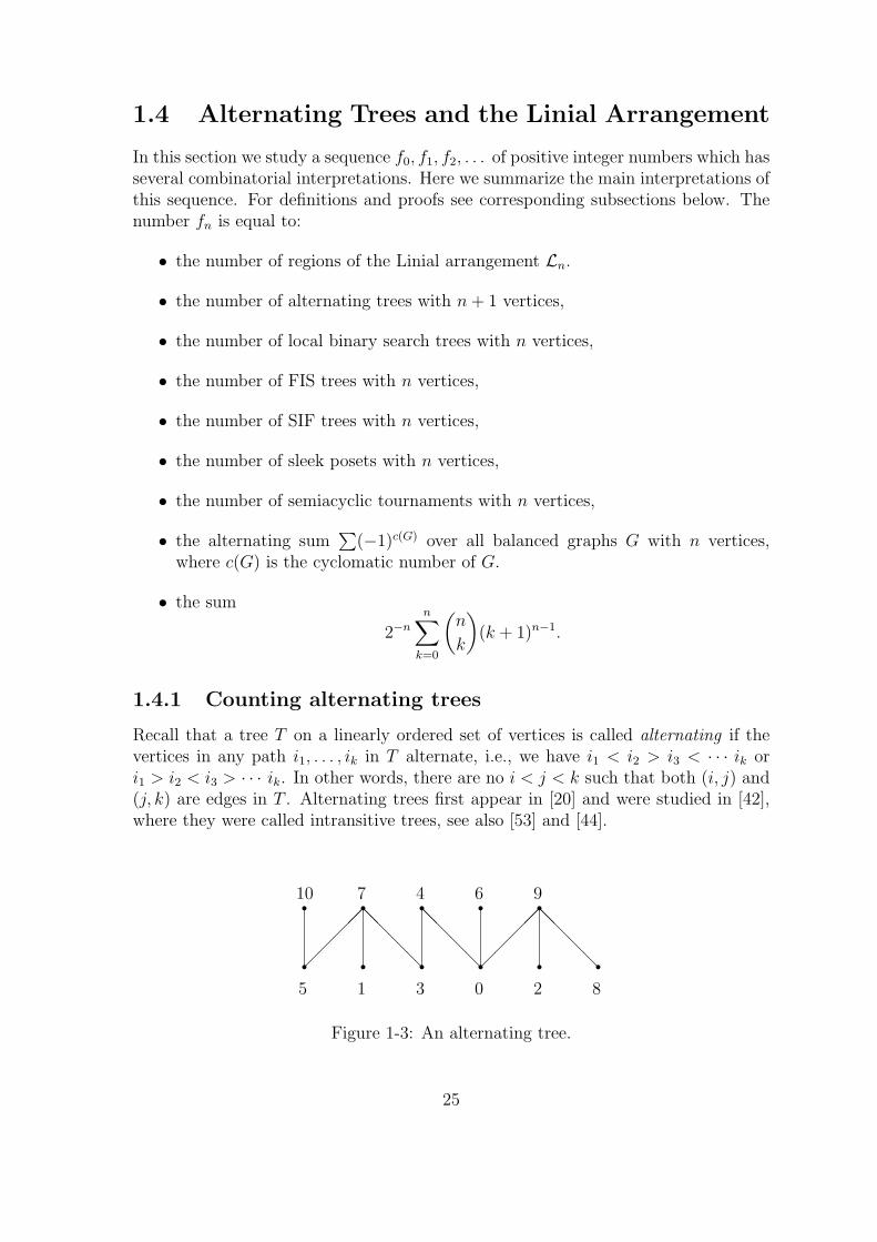
1.4.1 Counting alternating trees
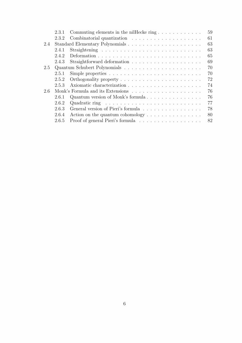
Recall that a tree T on a linearly ordered set of vertices is called alternating if thevertices in any path i1, . . . , ik in T alternate, i.e., we have i1 < i2 > i3 < · · · ik ori1 > i2 < i3 > · · · ik. In other words, there are no i < j < k such that both (i, j) and(j, k) are edges in T . Alternating trees first appear in [20] and were studied in [42],where they were called intransitive trees, see also [53] and [44].
r r r r rr r r r r
r
@@
@@@
@@
@@@
@@
@@@
01 23
4
5
67
8
910
Figure 1-3: An alternating tree.
25

Let fn be the number of alternating trees on the vertices 0, 1, 2, . . . , n, and let
f(x) =∑n≥0
fnxn
n!
be the exponential generating function for the sequence fn.
Theorem 1.4.1 [42, Theorems 1, 2] For n ≥ 1 we have
fn = 2−n
n∑k=0
(n
k
)(k + 1)n−1. (1.4.1)
The series f = f(x) satisfies the functional equation
f = ex(1+f)/2. (1.4.2)
The first few numbers fn are given below.
f0 f1 f2 f3 f4 f5 f6 f7 f8 f9 f10
1 1 2 7 36 246 2104 21652 260720 3598120 56010096
We need some extra notation. We say that i is a minimal vertex in an alternatingtree T if T contains an edge (i, j) for some j > i. A vertex is called maximal it is nota minimal vertex. If a vertex i is minimal (respectively, maximal) then for every edge(i, j) in T we have j > i (respectively, j < i). For example, the tree on Figure 1-3has minimal vertices 0, 1, 2, 3, 5, 8 and maximal vertices 4, 6, 7, 9, 10.
An alternating tree with a chosen vertex (root) is called a rooted alternating tree.If the root is a maximal vertex we call such a tree top-rooted.
Proof of Theorem 1.4.1 — First, we prove the formula (1.4.2).
Let fn be the number of all top-rooted alternating trees on the vertices 1, . . . , n.It is clear that, for n ≥ 2, the number fn is half the number of all rooted alternatingtrees on 1, . . . , n. Thus fn = nfn−1/2; also f1 = (f0 + 1)/2 = 1. We obtain thefollowing expression for the exponential generating function.
f(t) :=∑n≥1
fntn
n!= t(f(t) + 1)/2.
To get an alternating tree on the vertices 0, 1, . . . , n, take a forest of top-rootedtrees on the vertices 1, . . . , n and connect 0 to each root. By the exponential formula(e.g., see [23, p. 166]), we have
f(t) = ef(t).
This gives the formula (1.4.2).
26

Now we deduce (1.4.1). We have
f = t (1 + ef )/2.
By Lagrange’s inversion formula (see [23, p. 17]), we get
[tn]f =1
n 2n[λn−1]
(1 + eλ
)n=
1
n 2n
n∑k=0
(n
k
)kn−1
(n− 1)!,
where [tn]g denotes the coefficient of tn in g. Thus, for n ≥ 2,
fn−1 =1
n 2n−1
n∑k=0
(n
k
)kn−1. (1.4.3)
The formula (1.4.1) is equivalent to (1.4.3).
Remark 1.4.2 It is also possible to calculate the inverse of the function f(x). Itfollows from (1.4.2) that x = 2 ln(f)/(1 + f). One can expand it as the followingseries:
x = −∑n≥1
(1− f)n
n∑k=0
(n
k
)−1
.
1.4.2 Local binary search trees
A plane binary tree on the vertices 1, 2, . . . , n is called a local binary search tree (LBStree, for short) if for any vertex i the left child of i is less than i and the right child of iis greater than i. These trees were first considered by Ira Gessel [21], and were studiedin [42]. The name “local binary search tree” was suggested by Richard Stanley [53],see also [44].
r r r rr r r
r rr
@@
@@
@@
@@
@@
@@
@@
@@
@
@R
12
3
4
5
6
7
8 9
10
Figure 1-4: A local binary search tree.
Theorem 1.4.3 [42, Section 4.1] For n ≥ 1, the number of local binary search treeson the vertices 1, 2, . . . , n is equal to the number fn of alternating trees on the vertices0, 1, 2, . . . , n.
27

Proof — Let Rn be the set of rooted alternating trees on the vertices 0, 1, 2, . . . , n;and let Bn be the set of LBS trees on the vertices 0, 1, 2, . . . , n such that the root hasonly one child (left or right).
Clearly, |Rn| = (n + 1)fn. On the other hand, |Bn| is n + 1 times the number ofLBS trees on 1, 2, . . . , n. Indeed, for a LBS tree B ∈ Bn, the root r of B can be anyvertex 0 ≤ r ≤ n. Deleting the root r, we get a LBS tree T ′ on 0, 1, . . . , n \ r.Conversely, we can always reconstruct T if we know T ′ and r. In the case when theroof r′ of T ′ is less than r, we set r′ to be the left child of r; otherwise, if r′ < r, weset r′ to be the right child of r.
In order to prove Theorem 1.4.3, we construct a bijection φ : Rn → Bn. Let T bea rooted alternating tree T ∈ Rn. We construct the LBS tree B = φ(T ) using thefollowing simple procedure:
First, we orient the edges of T away from the root (e.g. the vertices adjacent tothe root are children of the root).
If v is a minimal vertex in T and i1 < i2 < · · · < il are the children of v in T(v < i1), then set i1 to be the right child of v in B, and ik+1 to be the right child ofik in B, for k = 1, 2, . . . , l − 1.
Analogously, if v is a maximal vertex in T and j1 > j2 > · · · > jl are the childrenof v in T (v > j1), then set j1 to be the left child of v in B, and jk+1 to be the leftchild of jk in B, for k = 1, 2, . . . , l − 1.
Clearly, the construction of the map φ is invertible. Thus φ is a bijection.
1.4.3 On stability and fickleness
Let On denote the set of rooted trees on the vertices 1, 2, . . . , n with edges orientedaway from the root.
We say that a path i1, i2, . . . , ik in a tree T ∈ On is stable if all edges (i1, i2),(i2, i3), (i3, i4), . . . ,(ik−1, ik) are oriented in the same direction, i.e., the path eitherapproaches the root, or goes away from the root.
We also say that a path j1, j2, . . . , jk is fickle if the vertices in it alternate, i.e, wehave j1 < j2 > j3 < . . . jk or j1 > j2 < j3 > . . . jk (cf. Section 1.4.1).
A tree T in On is called a “fickle is stable” tree (FIS tree) if every fickle path in Tis stable. Likewise, a tree T in On is called a “stable is fickle” tree (SIF tree) if everystable path in T is fickle.
Theorem 1.4.4 The number of FIS trees in On is equal to the number of SIF treesin On and is equal to the number fn of alternating trees on the vertices 0, 1, . . . , n.
Proof — First, we notice that a tree T from On is a FIS tree if and only if everyvertex i in T has none, one, or two children, and in the last case one of the childrenis less than i and the other is greater than i. We establish a simple bijection betweenFIS and local binary search trees. For a LBS tree, orient its edges away from theroot, and then forget the structure of a binary tree, i.e., forget which child was leftand which was right. We obtain a FIS tree. Thus, by merit of Theorem 1.4.3, the
28

number of FIS trees in On is equal to the number fn of alternating trees on thevertices 0, 1, 2, . . . , n.
SIF trees are more similar to alternating trees. In fact, they are almost alternatingin the sense that the condition for alternating tree is satisfied in every vertex but theroot (cf. Section 1.4.1).
A bijection between FIS trees and SIF trees can be constructed in a way similarto the proof of Theorem 1.4.3.
1.4.4 The Linial arrangement
Recall that Vn denotes the hyperplane (x1, . . . , xn) | x1 + · · · + xn = 0 in Rn.Consider the arrangement Ln of hyperplanes in Vn given by the equations
xi − xj = 1, 1 ≤ i < j ≤ n. (1.4.4)
This arrangement was first considered by Nati Linial and Shmulik Ravid. Theycalculated the numbers r(Ln) of regions of Ln and the Poincare polynomials PoinLn(q)for n ≤ 9.
AA
AA
AA
AA
AA
Figure 1-5: Seven regions of the Linial arrangement L3.
Our main result on the Linial arrangement is the following:
Theorem 1.4.5 [44, Theorem 8.2] The number r(Ln) of regions of Ln is equal tothe number fn of alternating trees on the vertices 0, 1, 2 . . . , n and, thus, to the numberof local binary search trees on 1, 2, . . . , n.
This theorem was conjectured by Richard Stanley, who used the numerical dataprovided by Linial and Ravid. In Section 1.5 we prove a more general result (seeTheorems 1.5.1 and Corollary 1.5.9). A different proof of Theorem 1.4.5 was latergiven by C. Athanasiadis [3].
Corollary 1.4.6 The Poincare polynomial of the Linial arrangement is equal to
PoinLn(q) =∑
T
qn−dT (0), (1.4.5)
29

where the sum is over all alternating trees T on the vertices 0, 1, . . . , n and dT (0)denotes the degree of the vertex 0 in T .
1.4.5 Balanced graphs
Let C = (c1, c2, . . . , cm) denote a cycle on a linearly ordered set of vertices which hasthe edges (c1, c2), (c2, c3), . . . , (cm−1, cm), (cm, c1). (Note that the sequence (c1, . . . , cm)is defined up to a cyclic permutation.) By convention, c0 = cm. We say that an index1 ≤ i ≤ m is an ascent in C if ci−1 < ci. Analogously, an index 1 ≤ j ≤ m is adescent if ci−1 > ci.
We say that a cycle C is balanced if the number of ascents in C is equal to thenumber of descents in C. A graph G is called balanced if every cycle in G is balanced.
A graph G on the vertices 1, 2, . . . , n corresponds to a subset of hyperplanesin (1.4.4): an edge (i, j) of G corresponds to the hyperplane xi − xj = 1, i < j.Geometrically, a graph is balanced if and only if the corresponding hyperplanes havea nonempty intersection.
Let c(G) denotes the cyclomatic number of G, i.e., the number of edges minus thenumber of vertices plus the number of connected components. Theorem 1.2.2 impliesthe following statement.
Corollary 1.4.7 For n ≥ 2, the number of regions of the Linial arrangement is equalto the alternating sum
r(Ln) =∑
G
(−1)c(G),
over all balanced graphs on the vertices 1, 2, . . . , n. The Poincare polynomial of thisarrangement is equal to
PoinLn(q) =∑
G
(−q−1)c(G) q|G|,
where again the sum is over all balanced graphs on 1, . . . , n and |G| is the number ofedges in G.
Orlik and Solomon’s result (Theorem 1.2.13) allows us to describe the cohomologyring H∗(CLn ,C) of the complement CLn to the complexified Linial arrangement interms of generators and relations.
Proposition 1.4.8 The cohomology ring H∗(CLn ,C) is canonically isomorphic tothe algebra (the Orlik-Solomon algebra) generated by eij = eji, 1 ≤ i, j ≤ n, eii = 0,subject to the following relations:
eijekl = −ekleij,
er1r2er2r3 . . . erm−1rmecmc1 = 0,
eabebceac − eabebcecd + eabeacecd − ebceacecd = 0,eacebcebd − eacebcead + eacebdead − ebcebdead = 0.
(1.4.6)
30
where i, j, k, l, r1, . . . , rm ∈ 1, . . . , n and 1 ≤ a < b < c < d ≤ n (cf. Figure 1-7).
Proof — By Theorem 1.2.13, the Orlik-Solomon algebra of the Linial arrangementis generated by the eij which are subject to the first two relation in (1.4.6) and alsothe relation:
p∑j=1
(−1)jec1c2ec2e2 . . . ecjcj+1. . . ecp−1cpecpc1 , (1.4.7)
where C = (c1, c2, . . . , cp) is a balanced cycle (cf. 1.2.14). We will show by inductionon p that the third and the fourth equations in (1.4.6) imply (1.4.7). If p = 4 thenC is a cycle of one of the four types C1, C2, C3, or C4 shown on Figure 1-7. Thus Cproduces one of the relations (1.4.6). If p > 4, then we can find r 6= s such that bothC ′ = (cr, cr+1, . . . , cs) and C ′′ = (cs, cs+1, . . . , cr) are balanced. The equation (1.4.7)for C is the sum of the corresponding equations for C ′ and C ′′.
This proposition is an analogue to Arnold’s description of the cohomology of thecomplement to complexified Coxeter arrangement (see Corollary 1.2.14).
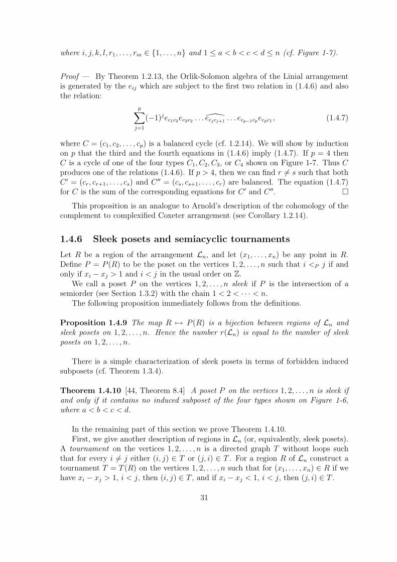
1.4.6 Sleek posets and semiacyclic tournaments
Let R be a region of the arrangement Ln, and let (x1, . . . , xn) be any point in R.Define P = P (R) to be the poset on the vertices 1, 2, . . . , n such that i <P j if andonly if xi − xj > 1 and i < j in the usual order on Z.
We call a poset P on the vertices 1, 2, . . . , n sleek if P is the intersection of asemiorder (see Section 1.3.2) with the chain 1 < 2 < · · · < n.
The following proposition immediately follows from the definitions.
Proposition 1.4.9 The map R 7→ P (R) is a bijection between regions of Ln andsleek posets on 1, 2, . . . , n. Hence the number r(Ln) is equal to the number of sleekposets on 1, 2, . . . , n.
There is a simple characterization of sleek posets in terms of forbidden inducedsubposets (cf. Theorem 1.3.4).
Theorem 1.4.10 [44, Theorem 8.4] A poset P on the vertices 1, 2, . . . , n is sleek ifand only if it contains no induced subposet of the four types shown on Figure 1-6,where a < b < c < d.
In the remaining part of this section we prove Theorem 1.4.10.First, we give another description of regions in Ln (or, equivalently, sleek posets).
A tournament on the vertices 1, 2, . . . , n is a directed graph T without loops suchthat for every i 6= j either (i, j) ∈ T or (j, i) ∈ T . For a region R of Ln construct atournament T = T (R) on the vertices 1, 2, . . . , n such that for (x1, . . . , xn) ∈ R if wehave xi − xj > 1, i < j, then (i, j) ∈ T , and if xi − xj < 1, i < j, then (j, i) ∈ T .
31

rr
rr
rr
rr
rrr
rrrr
ra
c
b
d
a
d
b
c
a
b
d
c
a
c
d
b
Figure 1-6: Obstructions to sleekness.
rr
r
C0
a
c
b rr
rr
C1
a b
c d
rr r
rC2
a b
cd rr
rr
C3
a
b c
d
rr
rr
C4
a
c b
d
AA
A
AAK
?J
JJ
JJ
6
JJ
JJ 6
JJ
JJJ
6
JJ
JJ 6
A
AA
A
AA
AAU
AAK
A
AA
A
AA
AAU
AAK
Figure 1-7: Ascending cycles.
Let C = (c1, . . . , cn) be a cycle; and let asc(C) denote the number of ascents anddes(C) denote the number of descents in C. We say that a cycle C is ascendingif asc(C) ≥ des(C). For example, the following cycles, shown on Figure 1-7, areascending: C0 = (a, b, c), C1 = (a, c, b, d), C2 = (a, d, b, c), C3 = (a, b, d, c), C4 =(a, c, d, b), where a < b < c < d.
We call a tournament T on 1, 2, . . . , n semiacyclic if it contains no ascendingcycles. In other words, T is semiacyclic if for any directed cycle C in T we haveasc(C) < des(C).
Proposition 1.4.11 A tournament T on 1, 2, . . . , n corresponds to a region R inLn, i.e., T = T (R), if and only if T is semiacyclic. Hence r(Ln) is the number ofsemiacyclic tournaments on 1, 2, . . . , n.
This fact was independently found by Shmulik Ravid.For any tournament T on 1, 2, . . . , n without cycles of type C0 we can construct
a poset P = P (T ) such that i <P j if and only if i < j and (i, j) ∈ T . Thefour ascending cycles C1, C2, C3, C4 in Figure 1-7 correspond to the four posets onFigure 1-6. Therefore, Theorem 1.4.10 is equivalent to the following result.
Theorem 1.4.12 [44, Theorem 8.6] A tournament T on the vertices 1, 2, . . . , n issemiacyclic if and only if it contains no ascending cycles of the types C0, C1, C2, C3,and C4 shown in Figure 1-7, where a < b < c < d.
Remark 1.4.13 This theorem is an analogue of a well-known fact that a tournamentT is acyclic if and only if it contains no cycles of length 3. For semiacyclicity we haveobstructions of lengths 3 and 4.
32

Proof — Let T be a tournament on 1, 2, . . . , n. Suppose that T is not semiacyclic.We will show that T contains a cycle of type C0, C1, C2, C3, or C4. Let C =(c1, c2, . . . , cm) be an ascending cycle in T of minimal length. If m = 3, or 4 then Cis of type C0, C1, C2, C3, or C4. Suppose that m > 4.
Lemma 1.4.14 We have asc(C) = des(C).
Proof — Since C is ascending, we have asc(C) ≥ des(C). Suppose asc(C) > des(c).If C has two adjacent ascents i and i+1 then (ci−1, ci+1) ∈ T (otherwise we have an as-cending cycle (ci−1, ci, ci+1) of type C0 in T ). Then C ′ = (c1, c2, . . . , ci−1, ci+1, . . . , cm)is an ascending cycle in T of length m− 1, which contradicts our assumption that Cis an ascending cycle of minimal length. So for every ascent i in C the index i+ 1 isa descent. Hence asc(C) ≤ des(C), and we get a contradiction.
We say that ci and cj are on the same level in C if the number of ascents betweenci and cj is equal to the number of descents between ci and cj.
Lemma 1.4.15 We can find i, j ∈ 1, 2, . . . ,m such that (a) i is an ascent and j isa descent in C, (b) i 6≡ j ± 1 mod m, and (c) ci and cj−1 are on the same level.
Proof — We may assume that for any 1 ≤ s ≤ m the number of ascents in 1, 2, . . . , sis greater than or equal to the number of descents in 1, 2, . . . , s (otherwise take somecyclic permutation of (c1, c2, . . . , cm)). Consider two cases.
1. There exists 1 ≤ t ≤ m − 1 such that ct and cm are on the same level. In thiscase, if the pair (i, j) = (1, t) does not satisfy conditions (a)–(c) then t = 2. On theother hand, if the pair (i, j) = (t + 1,m) does not satisfy (a)–(c) then t = m − 2.Hence, m = 4 and C is of type C1 or C2 shown in Figure 1-7.
2. There is no 1 ≤ t ≤ m − 1 such that ct and cm are on the same level. Then 2is an ascent and m − 1 is a descent. If the pair (i, j) = (2,m − 2) does not satisfy(a)–(c) then m = 4 and C is of type C3 or C4 shown on Figure 1-7.
Now we can complete the proof of Theorem 1.4.12. Let i, j be two numberssatisfying the conditions of Lemma 1.4.15. Then ci−1, ci, cj−1, cj are four distinctvertices such that (a) ci−1 < ci, (b) cj−1 > cj, (c) ci and cj−1 are on the same level,and (d) ci−1 and cj are on the same level. We may assume that i < j.
If (cj−1, ci−1) ∈ T then (ci−1, ci, . . . , cj−1) is an ascending cycle in T of lengthless than m, which contradicts the requirement that C is an ascending cycle on T ofminimal length. So (ci−1, cj−1) ∈ T . If ci−1 < cj−1 then (cj−1, cj, . . . , cm, c1, . . . , ci−1)is an ascending cycle in T of length less than m. Hence, ci−1 > cj−1.
Analogously, if (ci, cj) ∈ T then (cj, cj+1, . . . , cp, c1, . . . , ci) is an ascending cyclein T of length less than m. So (cj, ci) ∈ T . If ci > cj then (ci, ci+1, . . . , cj) is anascending cycle in T of length less than m. So ci < cj.
Now we have ci−1 > cj−1 > cj > ci > ci−1, and we get an obvious contradiction.We have shown that every minimal ascending cycle in T is of length 3 or 4 and
thus proved Theorem 1.4.12.
33

1.5 Truncated Affine Arrangements
In this section we study a general class of hyperplane arrangements which contains,in particular, the Linial and Shi arrangements.
Let a and b be two integers such that a+ b ≥ 2. Consider the hyperplane arrange-ment Aab
n in Vn = (x1, . . . , xn) ∈ Rn | x1 + · · ·+ xn = 0 given by
xi − xj = k, 1 ≤ i < j ≤ n, −a < k < b. (1.5.1)
We call Aabn truncated affine arrangement because it is a finite subarrangement of
the affine arrangement of type An−1 given by xi − xj = r, r ∈ Z.
1.5.1 Functional equations
Let fn = fabn be the number of regions of the arrangement Aab
n , and let
f(x) =∑n≥0
fnxn
n!(1.5.2)
be the exponential generating function for fn.
Theorem 1.5.1 [44, Theorem 9.1] Suppose a, b ≥ 0.
1. The generating function f = f(x) satisfies the following functional equation:
f b−a = ex · fa−fb
1−f . (1.5.3)
2. If a = b ≥ 1, then f = f(x) satisfies the equation:
f = 1 + x fa, (1.5.4)
Note that the equation (1.5.4) can be obtained from (1.5.3) by l’Hospital’s rule inthe limit b→ a.
In cases a = b and a = b ± 1 the functional equations (1.5.3) and (1.5.4) al-low to calculate the numbers fab
n explicitly. The following statement was proved byP. Headley [24].
Corollary 1.5.2 The number faan is equal to (a n)(a n− 1) · · · (a n− n+ 2).
The equation (1.5.3) is especially simple in the case a = b ± 1. We call thearrangement Aa,a+1
n the extended Shi arrangement. In this case we get:
Corollary 1.5.3 The number fn of regions of the extended Shi arrangement given by
xi − xj = −a+ 1,−a+ 2, . . . , a, 1 ≤ i < j ≤ n
is equal to fn = (a n + 1)n−1, and the exponential generating function f = f(x)satisfies the functional equation f = ex·fa
.
34

In order to prove Theorem 1.5.1 we need several new definitions. A graded graphis a graph is a triple G = (V,E, h), where V is a linearly ordered set of vertices, E isa set of (nonoriented) edges, and h is a function h : V → Z+ called grading. Thevertices v in V such that h(v) = r, r = 0, 1, 2, . . . , form the r-th level of G. Lete = (u, v) be an edge in G, u < v. We say that the slope of an edge e = (u, v), u < v,in E is the integer s(e) = h(v)−h(u). A graded graph G is of type (a, b) if the slopesof all edges in G are in the interval [−a + 1, b − 1] = −a + 1,−a + 2, . . . , b − 1.Analogously, we define graded trees, forests, and circuits of type (a, b).
Choose a linear order on the set (u, s, v) | u, v ∈ V, u < v, −a < s < b. LetC be a graded circuit of type (a, b). Every edge (u, v) in C corresponds to a triple(u, s, v), where s is the slope of the edge (u, v). Choose the edge e in C with theminimal triple (u, e, v). We say that C \ e is a broken circuit of type (a, b).
We say that a graded forest is planted if each connected component contains avertex on the 0-th level.
Proposition 1.5.4 The number fabn of regions of the arrangement (1.5.1) is equal to
the number of planted graded forests of type (a, b) on the vertices 1, 2, . . . , n withoutbroken circuits of type (a, b).
Proof — By Corollary 1.2.8, the number fn is equal to the number of A-coloredforests F without broken A-circuits. For an A-colored forest F , there is a uniqueplanted graded forest F = (V,E, h) with the same sets of vertices and edges and suchthat the slope s(e) of any edge e ∈ E is equal to the color of e in the forest F . Then
F is of type (a, b) and without broken circuits of type (a, b) if and only if F has nobroken A-circuits.
From now on we fix the lexicographical order on triples (u, s, v), i.e., (u, s, v) <(u′, s′, v′) if and only if u < u′, or (u = u′ and s < s′), or (u = u′ and s = s′ andv < v′). Note the order of u, s, and v! We call a graded tree T solid if T is of type(a, b) and T contains no broken circuits of type (a, b).
Let T be a solid tree on 1, 2, . . . , n such that the vertex 1 is on the r-th level. Whenwe delete the minimal vertex 1, the tree T decomposes into connected componentsT1, T2, . . . , Tm. Suppose that each component Ti is connected with 1 by an edge (1, vi)where vi is on the ri-th level.
Lemma 1.5.5 Let T, T1, . . . , Tm, v1, . . . , vm, and r1, . . . , rm be as above. The tree Tis solid if and only if (a) all T1, T2, . . . , Tm are solid, (b) for all i the ri-th level is theminimal nonempty level in Ti such that −a + 1 ≤ ri − r ≤ b − 1, and (c) the vertexvi is the minimal vertex on its level in Ti.
Proof — First, we prove that if T is solid then the conditions (a)–(c) hold. Condi-tion (a) is trivial, because if Ti contains a broken circuits of type (a, b) then T alsocontains this circuit. Assume that for some i there is a vertex v′i on the r′i-th levelin Ti such that r′i < ri and r′i − r ≥ −a + 1. Then the minimal chain in T thatconnects the vertex 1 with the vertex v′i is a broken circuit of type (a, b). Thus the
35

condition (b) holds. Now suppose that for some i the vertex vi is not the minimalvertex v′′i on its level. Then the minimal chain in T that connects the vertex 1 with v′′iis a broken circuit of type (a, b). Therefore, the condition (c) holds too.
Now assume that the conditions (a)–(c) are true. We prove that T is solid. Forsuppose not. Then T contains a broken circuit B = C \ e of type (a, b), where C isa graded circuit and e is its minimal edge. If B does not pass through the vertex 1then B lies in Ti for some i, which contradicts to the condition (a). We can assumethat B passes through the vertex 1. Since e is the minimal edge is C, e = (1, v) forsome vertex v′ on the level r′ in T . Suppose v ∈ Ti. If v′ and vi are on differentlevels in Ti then, by (b), ri < r. Thus the minimal edge in C is (1, vi) and not (1, v′).If v′ and vi are on the same level in Ti then, by (c), vi < v′. Again, the minimaledge in C is (1, vi) and not (1, v′). Therefore, the tree T contains no broken circuitof type (a, b), i.e., T is solid.
Let li be the minimal nonempty level in Ti, and let Li be the maximal nonemptylevel in Ti. By Lemma 1.5.5, the vertex 1 lies on the rth level for some li − b < r <Li + a ; for each r from this interval there is a unique way to connect Ti with thevertex 1 in the rth level.
Let pnkr denote the number of solid trees (not necessarily grounded) on the vertices1, 2, . . . , n which are located on levels 0, 1, . . . , k such that the vertex 1 is on the rthlevel, 0 ≤ r ≤ k.
Let
pkr(x) =∑n≥1
pnkrxn
n!, pk(x) =
k∑r=0
pkr(x).
By the exponential formula (see [23, p. 166]) and Lemma 1.5.5, we have
p′kr(x) = exp(bkr(x)), (1.5.5)
where bkr(x) =∑
n≥1 bnkrxn
n!and bnkr is the number of solid trees T on n vertices
located on the levels 0, 1, . . . , k such that at least one of the levels r − a+ 1, r − a+2, . . . , r + b− 1 is nonempty, 0 ≤ r ≤ k. The polynomial bkr(x) enumerates the solidtrees on the levels 1, 2, . . . , k minus trees on the levels 1, . . . , r− a and trees on levelsthe r + b, . . . , k. Thus we obtain
bkr(x) = pk(x)− pr−a(x)− pk−r−b(x).
By (1.5.5), we get
p′kr(x) = exp(pk(x)− pr−a(x)− pk−r−b(x)),
where p−1(x) = p−2(x) = · · · = 0, p0(x) = x, pk(0) = 0 for k ∈ Z. Hence
p′k(x) =k∑
r=0
exp(pk(x)− pr−a(x)− pk−r−b(x)).
36

Or, equivalently,
p′k(x) exp(−pk(x)) =k∑
r=0
exp(−pr−a(x)) exp(−pk−r−b)(x).
Let qk(x) = exp(−pk(x)). We have
q′k(x) = −k∑
r=0
qr−a(x) qk−r−b(x), (1.5.6)
q−1 = q−2 = · · · = 1, q0 = e−x, qk(0) = 1 for k ∈ Z.The following lemma describes the relation between the polynomials qk(x) and
the numbers of regions of the arrangement Aabn .
Lemma 1.5.6 The quotient qk−1(x)/qk(x) tends to∑
n≥0 fnxn
n!as k →∞.
Proof — Clearly, pk(x) − pk−1(x) is the exponential generating function for thenumbers of grounded solid trees of height less than or equal to k. By the exponentialformula (see [23, p. 166]) qk−1(x)/qk(x) = exp (pk(x)− pk−1(x)) is the exponentialgenerating function for the numbers of grounded solid forests of height less than orequal to k. The lemma obviously follows from Proposition 1.5.4.
All previous formulae and constructions are valid for arbitrary a and b. Now wetake advantage of the condition a, b ≥ 0. Let
q(x, y) =∑k≥0
qk(x)yk.
By (1.5.6), we obtain the following differential equation for q(x, y):
∂
∂xq(x, y) = − (ay + yaq(x, y)) ·
(by + ybq(x, y)
),
q(0, y) = (1− y)−1,
where ay := (1− ya)/(1− y).This differential equation has the following solution:
q(x, y) =by exp(−x · by)− ay exp(−x · ay)
ya exp(−x · ay)− yb exp(−x · by). (1.5.7)
Let us fix some small x. Since Q(y) := q(x, y) is an analytic function of y, then γ =γ(x) = limk→∞ qk−1/qk is the pole ofQ(y) closest to 0 (γ is the radius of convergence ofQ(y) if x is a small positive number). By (1.5.7), γa exp(−x·aγ)−γb exp(−x·bγ) = 0.Thus, by Lemma 1.5.6, f(x) =
∑n≥0 fn
xn
n!= γ(x) is the solution of the functional
equation
fa e−x · 1−fa
1−f = f b e−x · 1−fb
1−f ,
37

which is equivalent to (1.5.3).This completes the proof of Theorem 1.5.1.
1.5.2 Formulae for the characteristic polynomial
Let A = Aabn be the truncated affine arrangement given by (1.5.1). Consider the
characteristic polynomial χabn (q) of the arrangement Aab
n . Recall that it is equal toqn−1PoinAab
n(−q−1).
Let χab(x, q) be the exponential generating function
χab(x, q) = 1 +∑n>0
χabn−1(q)x
n/n! .
According to [53, Theorem 1.2], we have
χab(x, q) = f(−x)−q, (1.5.8)
where f(x) = χab(−x,−1) is the exponential generating function (1.5.2) for numbersof regions of Aab
n .Let S be the shift operator S : f(q) 7→ f(q − 1).
Theorem 1.5.7 [44, Theorem 9.7] Assume that 0 ≤ a < b. Then
χabn (q) = (b− a)−n(Sa + Sa+1 + · · ·+ Sb−1)n · qn−1. (1.5.9)
Proof — The theorem can be deduced from Theorem 1.5.1 and (1.5.8) (using, e.g.,Lagrange’s inversion formula).
There is an explicit formula for χaa(q). The following statement, found in [24], isnot hard to derive from Corollary 1.5.2.
Proposition 1.5.8 We have χaan (q) = (q + 1− an)(q + 2− an) · · · (q + n− 1− an).
We can analytically extend χabn (q) to complex values of a and b, since
χabn (q) =
(Sa (Sb−a − 1)/((S − 1)(b− a))
)n · qn−1
In the limit b→ a, application of the l’Hospital’s rule results in the expression8
χaan (q) =
(Sa lnS
S − 1
)n
· qn−1.
8Comparing these two expressions for χaa(q), we obtain the formula(D
eD − 1
)n
· qn−1 = (q − 1)(q − 2) · · · (q − n + 1) ,
where D = − ln(S) = d/dq. This formula yields an identity that involves the Bernoulli numbers,which are coefficients of the Taylor expansion of x/(ex − 1), and the Stirling numbers of the firstkind.
38

There are several equivalent ways to reformulate Theorem 1.5.7, as follows:
Corollary 1.5.9 Let r = b− a.
1. We haveχab
n (q) = r−n∑
(q − φ(1)− · · · − φ(n))n−1 ,
where the sum is over all functions φ : 1, . . . , n → a, . . . , b− 1.
2. We have
χabn (q) = r−n
∑s, l≥0
(−1)l(q − s− an)n−1
(n
l
)(s+ n− rl − 1
n− 1
).
3. We have
χabn (q) = r−n
∑(n
n1, . . . , nr
)(q − an1 − · · · − (b− 1)nr)
n−1 ,
where the sum is over all nonnegative integers n1, n2, . . . , nr such that n1 +n2 +· · ·+ nr = n.
Examples:
1. The Shi arrangement is the arrangement A12n given by
xi − xj = 0, 1, 1 ≤ i < j ≤ l + 1. (1.5.10)
By Corollary 1.5.9.1, we get the following known formula (see [48, 49])
χ1 2n (q) = (q − n)n−1.
2. More generally, for the extended Shi arrangement Aa,a+1n , given by
xi − xj = −a+ 1,−a+ 2, . . . , a, 1 ≤ i < j ≤ l + 1,(1.5.11)
we have (cf. Corollary 1.5.3)
χa, a+1n (q) = (q − an)n−1.
3. For the Linial arrangement Ln = A02n (see Section 1.4), Corollary 1.5.9.3 gives
χ0 2n (q) = 2−n
n∑k=0
(n
k
)(q − k)n−1, (1.5.12)
(cf. Theorem 1.4.5)
39

4. More generally, for the arrangement Aa, a+2n , we have
χa, a+2n (q) = 2−n
n∑k=0
(n
k
)(q − an− k)n−1.
Formula (1.5.12) for the characteristic polynomial χ0 2n (q) was earlier obtained
by C. Athanasiadis [3, Theorem 5.2]. He used a different approach based on aninterpretation of the value of χn(q) for sufficiently large primes q.
1.5.3 Roots of the characteristic polynomial
Theorem 1.5.7 has one surprising application concerning the location of roots of thecharacteristic polynomial χab
n (q)We start with the case a = b. One can reformulate Proposition 1.5.8 in the
following way:
Corollary 1.5.10 The roots of the polynomial χaan (q) are the numbers an − 1, an −
2, . . . , an− n+ 1 (each with multiplicity 1). In particular, the roots are symmetric toeach other with respect to the point (2a− 1)n/2.
Now assume that a 6= b. We will prove the following “Riemann hypothesis.”
Theorem 1.5.11 [44] All the roots of the characteristic polynomial χabn (q) of the
truncated affine arrangement Aabn , a 6= b, have real part equal to (a+ b−1)n/2. They
are symmetric to each other with respect to the point (a+ b− 1)n/2.
Thus in both cases the roots of the polynomial χabn (n) are symmetric to each other
with respect to the point (a + b − 1)n/2, but in the case a = b all roots are real,whereas in the case a 6= b the roots are on the same vertical line9 in the complexplane C. Note that in the case a = b − 1 the polynomial χab
n (q) has only one rootan = (a+ b− 1)n/2 with multiplicity n− 1.
The following lemma is implicit in a paper of Auric [4] and also follows from aproblem posed by Polya [40] and solved by Obreschkoff [37] (repeated in [41, ProblemV.196.1, pp. 70 and 251]).
Lemma 1.5.12 Suppose that a polynomial f(q) ∈ C[q] is such that every zero hasreal part a, and let λ be a complex number satisfying |λ| = 1. Then every zero of thepolynomial g(q) = (S − λ)f(q) = f(q − 1)− λf(q) has real part a+ 1/2.
Proof of Theorem 1.5.11. — All the zeros of the polynomial qn−1 have real part 0.The operator (Sa + Sa+1 + · · ·+ Sb−1) can be written as
Sa(S − λ1) · · · (S − λb−a−1),
9Let χn(q) = χabn (q − (a + b − 1)n/2), its roots are purely imaginary. The following interlacing
property of roots seems also to be valid: Between any two roots of χn(q) there is a root of χn−1(q).
40

where each λj is a complex number of absolute value one. The proof now follows fromTheorem 1.5.7 and Lemma 1.5.12.
1.6 Asymptotics and Random Trees
1.6.1 Characteristic polynomials and trees
According to Theorem 1.5.7, the characteristic polynomial of a truncated affine ar-rangement can be easily expressed using the shift operator: S : f(q) 7→ f(q − 1).Let us also introduce the differentiation operator: D : f(q) 7→ df/dq. Then Taylor’stheorem can be stated as
exp(−D) = S.
Consider the exponential power series
h(t) = h0 + h1t+ h2t2/2! + · · ·+ hkt
k/k! + . . . ,
where the hi are some numbers and h0 is nonzero.Generalizing the expression (1.5.9), we define the polynomials fn(q), n > 0, by
the formula
fn(q) = (h(D))n qn−1. (1.6.13)
The polynomials fn(q) are correctly defined even if the series h(t) does not converge,since the expression for fn(q) involves only a finite sum of nonzero terms.
Let Tn be the set of trees on the vertices 0, 1, 2, . . . , n. We will assume that theedges of trees are oriented away for the root at the vertex 0. By di = di(T ) we denotethe outdegree of a vertex i in a tree T ∈ Tn. Define the weight of T by
wq(T ) = qd0−1hd1hd2 . . . hdn .
Proposition 1.6.1 1. The polynomial fn(q) is the weight enumerator for trees onn+ 1 vertices, i.e.
fn(q) =∑T∈Tn
wq(T ).
2. The coefficient of qk in fn(q) is equal to∑hk1 . . . hkn
(n− 1
k, k1, . . . , kn
),
where the sum is over all k1, . . . , kn ≥ 0 such that k + k1 + · · ·+ kn = n− 1.
Proof — Let D(k) = Dk/k!. Then, for k > 0, we have
D(k) qm =
(m
k
)qm−k,
41

if m ≥ k and 0 otherwise. By (1.6.13), we have
fn(q) = h(D)n qn−1 = h(D)n−1∑k1≥0
hk1D(k1) qn−1
= h(D)n−1∑k1≥0
hk1
(n− 1
k1
)qn−1−k1 = . . .
=∑
k,k1,...,kn≥0
hk1 . . . hkn
(n− 1
k, k1, k2, . . . , kn
)qk
where k = n − 1 − k1 − · · · − kn. Using Prufer’s coding [45], we obtain the firststatement of the theorem.
Let
f(z, q) = 1 + q∑n≥1
fn(q)zn
n!.
Consider also the weighting on trees T ∈ Tn given by
w(T ) = hd0hd1 . . . hdn .
Let gn =∑
T∈Tnw(T ) be the weighted sum of the trees, and let
g(x) =∑n≥0
gnxn+1
n!
be the exponential generating function for the gn. Note that ngn = fn+1(0).
Proposition 1.6.2 We have f(x, q) = exp(q g(x)). The series g = g(z) satisfies thefunctional equation
g = xh(g). (1.6.14)
The statement of the theorem is proved by a standard argument with the expo-nential formula.
1.6.2 Random trees
In this section we calculate the distribution of degrees of vertices of a “random infinitetree.” We will need these calculations in Section 1.6.3.
We use the notation of the previous section with the assumption that h0, h1, h2, . . .are nonnegative integer numbers, and h0 > 0.
Let I be the set of indices n for which gn > 0. If hi is nonzero for some i ≥ 1,then I is an infinite set. For n ∈ I, consider the distribution on the set of trees onn + 1 vertices given by P (T ) = w(T )/gn. Let Pn(k) denote the probability that a
42

random vertex of a random tree has outdegree k, i.e.,
Pn(k) =1
(n+ 1) gn
∑T∈Tn
mk(T ) w(T ),
where mk(T ) is the number of vertices in T with outdegree k. Also let P (k) =limn→∞ Pn(k), where the limit is taken over n ∈ I.
Here is an example when we need to be careful about the index set. Assume thath2m = 1 and h2m+1 = 0, for m ≥ 0, then gm = 0 for odd n. In this case we have totake the limit over even n.
We can interpret P (k) as the probability that a random vertex of a random infinitetree has outdegree k.
Theorem 1.6.3 Assume that the series h(t) converges, h′(t) is unbounded on theinterval (0,+∞), and t = α is the minimal positive solution of the equation
t = h(t)/h′(t) . (1.6.15)
Then
P (k) =hk α
k
h(α) k!.
Before we prove this statement, consider several examples. In the case whenhk = 1, k ≥ 0, we obtain the uniform distribution on trees.
Corollary 1.6.4 The outdegrees of a random infinite tree have Poisson distribution:
P (k) = e−1/k! .
Proof — We have h(t) = et. The equation t = et/et has a unique solution t = 1.
Assume that h2m = 1 and h2m+1 = 0, m ≥ 0. We have the uniform distributionon trees with even outdegrees. We will call such trees even.
Corollary 1.6.5 The outdegrees of a random infinite even tree have the followingdistribution:
P (2m) = P (0)α2m/(2m)! ,
where α = 1.199678640257733 . . . is a unique positive solution of the equation
e2t =t+ 1
t− 1, t > 1, (1.6.16)
and P (0) = 1/ cosh(α) = 0.552434124530883 . . . .
Proof — In this case h(t) = cosh(t). The equation t = cosh(t)/ sinh(t) is equivalentto (1.6.16).
43

Proof of Theorem 1.6.3 — Let
p(x) =∑n≥0
(n+ 1)Pn(k) gnxn/n! ,
d(x) =∑n≥0
(n+ 1) gnxn/n! .
Then, by definition, P (k) is the limit of ratios of coefficients of xn in p(x) and d(x)as n → ∞. First, we note that if x0 > 0 is the minimal positive pole of both p(x)and d(x), then P (k) = limx→x0 p(x)/d(x).
We have d(x) = g′(x). By (1.6.14),
d(x) = h(g) + xh′(g)d(x) ,
d(x) =h(g)
1− xh′(g). (1.6.17)
Let g(k)(x, y) be the following exponential generating function
g(k)(x, y) =∑n≥0
∑T∈Tn
w(T )ymk(T )xn+1/n!.
Clearly,
p(x) = x−1 ∂g(k)
∂y
∣∣∣∣y=1
(x).
The function g(k) satisfies the equation:
g(k) = x (h(g(k)) + (y − 1)hkgk(k)/k!).
Then
p(x) = xh′(g) p(x) + hkgk/k! ,
p(x) =hkg
k
k! (1− xh′(g)). (1.6.18)
Let x0 be the minimal positive number such that
1− x0 h′(g(x0)) = 0. (1.6.19)
Then x0 is the minimal positive pole of p(x) as well as of d(x). Assume not, thenthere is a pole x1 of g(x) (or h(g(x))) such that 0 < x1 ≤ x0 (cf. (1.6.17) and (1.6.18)).Since h′(t) is unbounded, there is a root of (1.6.19) between 0 and x1. Contradiction.
Therefore, by earlier remark,
P (k) = limx→x0
p(x)
d(x)=
hk αk
h(α) k!,
44

where α = g(x0). The equation (1.6.15) for α follows from (1.6.14) and (1.6.19).
1.6.3 Asymptotics of characteristic polynomials
It is convenient to introduce the following shift the characteristic polynomial of theLinial arrangement:
bn(q) = 2n−1χ02n ((q + n)/2).
Then, by Theorem 1.5.7,
bn(q) =
(S + S−1
2
)n
qn−1 = cosh(D)n qn−1.
The first ten polynomials bn(q) are given below:
b1(q) = 1,
b2(q) = q,
b3(q) = q2 + 3,
b4(q) = q3 + 12q,
b5(q) = q4 + 30q2 + 65,
b6(q) = q5 + 60q3 + 480,
b7(q) = q6 + 105q4 + 1995q2 + 3787,
b8(q) = q7 + 168q5 + 6160q3 + 41216q,
b9(q) = q8 + 252q6 + 15750q4 + 242172q2 + 427905,
b10(q) = q9 + 360q7 + 35280q5 + 1021440q3 + 6174720q,
Recall that α = 1.199678640 . . . is a unique solution of the equation
e2t = (t+ 1)/(t− 1), t > 1. (1.6.20)
Theorem 1.6.6 The functions b2m(q)/b′2m(0) converges to a limit beven(q) as m goesto infinity and
beven(q) = sinh(αq)/α.
Theorem 1.6.7 The functions b2m+1(q)/b2m+1(0) converges to a limit bodd(q) as mgoes to infinity and
bodd(q) = cosh(αq).
Consider the numbers bn,k given by
bn(q) = bn,n−1qn−1 + bn,n−3q
n−3 + bn,n−5qn−5 + bn,n−7q
n−7 + . . . ,
and bn,k = 0 if n − k is even. Note that bn,n−1 = 1. Also let bn = bn,n−1 + bn,n−3 +bn,n−5 + · · · = bn(1).
45

For example, b1, b2, . . . , b10 = 1, 1, 4, 13, 96, 541, 588, 47545, 686080, 7231801.We say that T ∈ Tn is an even tree if the outdegrees d1, d2, . . . , dn of all vertices T
(the root 0 excluded) are even. Equivalently, the degrees of all vertices in T but theroot are odd. Such trees are also called odd degree trees.
By Propositions 1.6.1 and 1.6.2, we obtain the following statement.
Corollary 1.6.8 1. The number bn,k is equal to the number of all even trees onthe vertices 0, 1, . . . , n such the degree of the root 0 is equal to k + 1.
2. The number bn,k is equal to the sum of polynomial coefficients(
n−1k,k1,...,kn
)over
all even k1, . . . , kn ≥ 0 such that k + k1 + · · ·+ kn = n− 1.
3. Let
b(x, q) = 1 + q∑n≥1
bn(q)xn
n!.
g(x) =∑m≥0
b2mx2m+1
(2m)!
Then b(x, q) = exp(q g(x)). The function g = g(x) satisfies the functionalequation
g = x cosh(g).
Proof of Theorems 1.6.6 and 1.6.7 — It is enough to show that b2m,2r+1/b2m,2r+3
tend to α−2(2r+3)(2r+2), and that b2m+1,2r/b2m+1,2r+2 tends to α−2(2r+2)(2r+1)as m goes to infinity, where α is given by (1.6.20).
By Corollary 1.6.8.2, we have bn,k =(
n−1k
)cn,k, where
cn,k =∑
k1,...,kn
(n− k − 1
k1, k2, . . . , kn
)the sum over all even nonnegative k1, k2, . . . , kn such that
∑ki = n− k − 1.
Asymptotically,bn,k
bn,k+2
≡ (k + 2)(k + 1)cn,k
n2 cn,k+2
as n goes to the infinity with preserving its parity.Let M
(1)n,k be the set of maps φ : 1, . . . , n− k− 1 → 1, . . . , n such that |φ−1(i)|
is even for i = 1, . . . , n. By definition, cn,k is equal to |M (1)n,k|.
Analogously, denote by M(2)n,k the set of maps ψ : 1, . . . , n− k − 1 → 1, . . . , n
such that |ψ−1(i) ∩ 1, . . . , n − k − 3| is even for i = 1, . . . , n. It is clear that
n2 cn,k+2 = |M (2)n,k|.
Also let M(3)n,k ⊂ M
(2)n,k be the subset of maps ψ : 1, . . . , n − k − 1 → 1, . . . , n
such that ψ(k) ∈ ψ(n− k − 2), ψ(n− k − 1) for some k ∈ 1, . . . , n− k − 3 .
46

The simple identity ∑l≥0
(m
2l
)=∑l≥0
(m
2l + 1
), m > 0
implies that |M (1)n,k| = |M (3)
n,k|.Recall that P (0) = 0.552434 . . . is the “probability that a random vertex of a
random even tree has outdegree 0,” which is calculated in Corollary 1.6.5. Thenumber of elements in M
(2)n,k \M
(3)n,k is asymptotically equal to α |M (2)
n,k|, as n goes toinfinity (k is fixed). The proof of Theorems 1.6.6 and 1.6.7 now easily follows.
47
48

Chapter 2
Quantum Cohomology of FlagManifolds
This part of my thesis contains the results of [17] obtained in collaboration withSergey Fomin and Sergei Gelfand as well as the results of [43]. Our notation andexposition of results are close (though not always identical1) to that of [17].
2.1 Introduction
The purpose to this chapter is to present an algebro-combinatorial method for calcula-tion of 3-point Gromov-Witten invariants of complex flag manifolds and to investigateits various consequences. These invariants are structure constants of the quantumcohomology ring of the flag manifold. In a special case, they are the Littlewood-Richardson coefficients, which are the intersection numbers of Schubert varieties.
A central open problem of Schubert calculus is to find an explicit rule for calcula-tion of the Littlewood-Richardson coefficients of flag manifolds that would imply thatthey are integer nonnegative numbers. For example, one would like to have a combi-natorial construction of a set, whose number of elements is equal to the correspondingLittlewood-Richardson coefficient. We extend this problem to that of finding a rulefor the Gromov-Witten invariants. This extension may lead to a way to solve theproblem, since the Gromov-Witten invariants seem to possess more symmetries.
We give below a brief account of definitions and results related to the classical andquantum cohomology rings of complex flag manifolds as well as formulate our mainresults. Although many of the constructions can be carried out in a more generalsetup of an arbitrary semisimple Lie group, only the case of type An−1 is considered.
Let Fln denote the manifold of complete flags of subspaces in the n-dimensionallinear space Cn. There are several ways to describe the cohomology ring H∗(Fln ,Z)of the flag manifold.
The additive structure of H∗(Fln,Z) can be obtained from the decompositionof Fln into Schubert cells, which are indexed by the elements of the symmetric
1One apparent difference is our extensive use of nilHecke rings.
49

group Sn. According to classical Ehresmann’s result [15], the Schubert classes σw,w ∈ Sn, corresponding to these cells, form an additive Z-basis of the cohomology ringof Fln.
The multiplicative structure of H∗(Fln,Z) can be recovered from Borel’s theo-rem [7], which says that the cohomology of Fln is isomorphic, as a graded ring, tothe quotient of the polynomial ring:
H∗(Fln,Z) ∼= Z[x1, x2, . . . , xn] / 〈en1 , e
n2 , . . . , e
nn〉 , (2.1.1)
where eni is the i-th elementary symmetric polynomial in x1, . . . , xn and 〈en
1 , . . . , enn〉
denotes the ideal generated by the eni . (The somewhat unusual notation with upper
indices will be handy when we use elementary symmetric polynomials in differentnumber of variables.) The isomorphism is given by mapping the generators x1, . . . , xn
into the first Chern classes of n standard line bundles on Fln , which are 2-dimensionalcohomology classes.
A way to relate these two approaches to the cohomology ring was found by Bern-stein, Gelfand, and Gelfand in [5] and Demazure [14], using divided difference op-erators. Later, Lascoux and Schutzenberger [31] further clarified this theory by in-troducing Schubert polynomials Sw ∈ Z[x1, . . . , xn], w ∈ Sn, whose images in thequotient (2.1.1) represent the Schubert classes σw . An algebraic formalization and ex-tension of Bernstein-Gelfand-Gelfand operators was given by Kostant and Kumar [30],who studied the nilHecke ring.
A quantum version2 of the story surfaced when mathematicians, motivated byideas of physicists [60, 56], introduced the quantum cohomology ring QH∗(X,Z), fora Kahler manifold X (see, e.g., [46, 28, 19] and references therein). This ring isa deformation of the classical cohomology ring, its structure constants are 3-pointGromov-Witten invariants, which count the numbers of certain rational curves andplay a role in enumerative algebraic geometry.
As a vector space, the quantum cohomology ring QH∗(Fln,Z) of the flag manifoldis essentially the same as the usual cohomology, and can be described via Ehresmann’sresult. More precisely,
QH∗(Fln,Z) ∼= H∗(Fln,Z)⊗ Z[q1, . . . , qn−1].
However, the multiplicative structure in QH∗(Fln,Z) is different comparing to thatof the classical cohomology and specializes to the latter when q1 = · · · = qn−1 = 0.
A quantum analogue of Borel’s theorem was suggested by Givental and Kim [22],and then justified by Kim [27] and Ciocan-Fontanine [12]. Let En
1 , En2 , . . . , E
nn ∈
Z[x1, . . . , xn; q1, . . . , qn−1] be the coefficients of the characteristic polynomial
det(1 + λCn) = 1 +n∑
i=1
Eni λ
i (2.1.2)
2The reader should not be confused by our use of the word “quantum.” The quantization thatwe discuss in this chapter does not seem to be related, at least at first glance, to quantum groups.
50

of the following 3-diagonal matrix
Cn =
x1 q1 0 · · · 0 0−1 x2 q2 · · · 0 00 −1 x3 · · · 0 0...
......
. . ....
...0 0 0 · · · xn−1 qn−1
0 0 0 · · · −1 xn
. (2.1.3)
The Enk are certain q-deformations of the elementary symmetric polynomials en
k andare equal to them when q1 = · · · = qn−1 = 0.
Givental, Kim, and Ciocan-Fontanine showed that the quantum cohomology ringof the flag manifold is isomorphic, as an algebra over Z[q1, . . . , qn−1], to the quotient
QH∗(Fln,Z) ∼= Z[x1, . . . , xn; q1, . . . , qn−1] / 〈En1 , . . . , E
nn〉 . (2.1.4)
A natural problem is to find the expansion of the quantum product σu ∗σw of twoSchubert classes in the basis of Schubert classes, where “∗” denotes the multiplica-tion in the quantum cohomology ring. Equivalently, one would like to calculate theGromov-Witten invariants of the flag manifold. We solve this problem, or at leastreduce it to combinatorics. Our construction provides the quantum analogue of theresult of Bernstein, Gelfand, and Gelfand and corresponding deformation of Schu-bert polynomials of Lascoux and Schutzenberger. The solution to the above problemis essentially combinatorial, and only relies on a few geometrical properties of thequantum cohomology, which are obvious3 from its definition.
Let I be a sequence (i1, . . . , in−1) such that 0 ≤ ik ≤ k for all k. Define standardelementary polynomial eI and quantum standard elementary polynomial EI by theformulas
eI = ei1...in−1 = e1i1 · · · en−1in−1
, (2.1.5)
EI = Ei1...in−1 = E1i1· · ·En−1
in−1, (2.1.6)
where, by convention, ek0 = Ek
0 = 1. The cosets of (quantum) standard elementarypolynomials form linear bases in the quotient rings (2.1.1) and (2.1.4).
For w ∈ Sn, the Schubert polynomial Sw can be uniquely expressed as a lin-ear combination
∑αI eI of standard elementary polynomials. Define the quantum
Schubert polynomial Sqw ∈ Z[x1, . . . , xn; q1, . . . , qn−1] by
Sqw =
∑I
αI EI . (2.1.7)
Our result on the quantum cohomology of the flag manifolds can now be statedas follows (cf. Theorem 2.3.6).
3almost
51

Theorem 2.1.1 [17, Theorem 1.2] The image of a quantum Schubert polynomial Sqw
in the quotient ring (2.1.4) represents the Schubert class σw in QH∗(Fln,Z).
We also prove the quantum version of Monk’s formula, which generalizes theclassical Monk’s result [36]. Let sij be the element of Sn that transposes i and j, andlet si = si i+1, i = 1, . . . , n − 1, be the Coxeter generators of Sn. Let us also denoteqij = qiqi+1 · · · qj−1, for i < j.
Theorem 2.1.2 (Quantum Monk’s formula) [17, Theorem 1.3] For w ∈ Sn and1 ≤ k < n, the quantum product of Schubert classes σsk
and σw is given by
σsk∗ σw =
∑σwsab
+∑
qcd σwscd, (2.1.8)
where the first sum is over all transpositions sab such that a ≤ k < b and `(wsab) =`(w) + 1 (as in the classical Monk’s formula), and the second sum is over all trans-positions scd such that c ≤ k < d and `(wscd) = `(w)− `(scd) = `(w)− 2(d− c) + 1.
The formula (2.1.8) unambiguously determines the multiplicative structure of thequantum cohomology ring QH∗(Fln,Z) with respect to the basis of Schubert classes,since this ring is generated by the 2-dimensional classes σsk
.Our proof of Theorems 2.1.1 and 2.1.2 is based on the study of certain pairwise
commuting elements in the nilHecke ring. They allow us to (combinatorially) deforma commutative ring4 equipped with an action of the nilHecke ring. For instance, thedeformation of the cohomology ring of Fln is shown to be equal to the correspondingquantum cohomology ring.
Another approach to the (quantum) cohomology ring of the flag manifold wasrecently highlighted by Fomin and Kirillov in [18], where they studied the ring En
generated by the elements τij, 1 ≤ i < j ≤ n, subject to the relations
τij τij = 0 , (2.1.9)
τij τjk = τjkτik + τikτij ,
τjkτij = τikτjk + τij τik ,
τij τkl = τkl τij , for distinct i, j, k, and l .
This ring also contains a family of pairwise commuting “Dunkl” elements defined by
θi = −∑j<i
τji +∑k>i
τik i = 1, 2, . . . , n . (2.1.10)
Fomin and Kirillov demonstrated that the subring generated by the θi is isomor-phic to the cohomology ring of Fln. The isomorphism is given by explicitly specifyingthat the generator xi of (2.1.1) maps to θi.
4It deformation is also a commutative ring.
52

A deformation Eqn of the ring En was also given in [18], along with the conjec-
ture that its subring generated by the Dunkl elements is isomorphic to the quantumcohomology of the flag manifold. We provide a proof to this statement.
The ring Eqn is generated by the elements τij, 1 ≤ i < j ≤ n, subject to the same
relations with the τij replaced by the τij, but instead of the relation (2.1.9) we have
τij τij =
qi for j = i+ 10 otherwise.
(2.1.11)
Define the elements θi in the ring Eqn by the same formula (2.1.10) with the τij replaced
by the τij. We can now formulate our result as follows.
Theorem 2.1.3 [43, Corollary 3.5] [18, Conjecture 13.4] The pairwise commutingelements θ1, . . . , θn generate the subring in Eq
n isomorphic to the quantum cohomologyring of Fln. The isomorphism is given by specifying that the generator xi of (2.1.4)maps to θi.
We deduce this theorem from a certain general Pieri-type formula. The latter alsoimplies Pieri’s formula for the product in H∗(Fln,Z) of any Schubert class σw withthe class σc(k,m), where c(k,m) = sm−k+1sm−k+2 · · · sm. This rule was first formulatedby Lascoux and Schutzenberger [31] and proved geometrically by Sottile [50].
Another corollary is an analogue of Pieri’s formula for the quantum cohomologyring that was recently proved by Ciocan-Fontanine [13], using nontrivial algebro-geometric techniques. By contrast, our proof is combinatorial, and does not relyupon geometry at all—once quantum Monk’s formula (2.1.8) is established. Ourproof seems to be new even in the classical case.
In the rest of Introduction we present the general outline of this chapter. InSection 2.2, we review the necessary background from the theory of classical coho-mology of the flag manifold, the nilHecke ring, and Schubert polynomials, togetherwith quantum cohomology definitions. In Section 2.3, we give a combinatorial con-struction of quantization for a ring equipped with an action of the nilHecke ring.This construction is based on a certain family of maximal commutative subrings inthe nilHecke ring. In Section 2.4, we study the standard elementary polynomials andtheir quantum analogues. In Section 2.5, we define the quantum Schubert polynomi-als and give a combinatorial proof of their orthogonality property (Theorem 2.5.5).We prove an axiomatic characterization of these polynomials (Theorem 2.5.7), whichimplies Theorem 2.1.1. We also conjecture there even stronger statement (Conjec-ture 2.5.8). The proof of quantum Monk’s formula, which is given in Section 2.6,becomes now almost tautological. In that section we also prove a general Pieri-typeformula (Theorem 2.6.3). As corollaries we obtain Theorem 2.1.3 as well as severalother conjectures from [18].
53

2.2 Background
2.2.1 Flag manifold and Schubert cells
We start with a short review of the basic results [5, 7] on the classical cohomology ofthe flag manifold. Most of the statements below can be extended to any semisimpleLie group.
Let Fln be the flag manifold whose points are the complete flags of subspaces
U. = (U1 ⊂ U2 ⊂ · · · ⊂ Un = Cn) , dimUi = i , (2.2.1)
in the n-dimensional linear space Cn. This is a projective algebraic variety.A description of the additive structure of the cohomology ring H∗(Fln ,Z) is based
on a decomposition of Fln into even-dimensional cells indexed by the elements of thesymmetric group Sn and called Schubert cells. These cells are described in terms of arelative position of a flag U. with respect to a fixed reference flag V. ∈ Fln , as follows.
Let v1, . . . , vn be a basis in Cn, and let Vr denote the r-dimensional subspacespanned by v1, v2, . . . , vr . For w ∈ Sn , define the Schubert cell Ωo
w as the set of allflags U. ∈ Fln such that, for all k, r ∈ 1, . . . , n,
dim(Uk ∩ Vr) = #1 ≤ i ≤ k , n+ 1− w(i) ≤ r .
The cell Ωow is homeomorphic to Rn(n−1)−2l, where l = `(w) is the length of w
(the number of inversions). The collection of all Ωow form a cell decomposition
of Fln. The Schubert variety Ωw is the closure of Ωow in Zariski topology. Let
[Ωw] ∈ Hn(n−1)−2l(Fln ,Z) be the fundamental cycle of Ωw . Define the Schubert class
σw = [Ωw]∗ ∈ H2l(Fln ,Z)
as the cohomology class corresponding to the fundamental cycle [Ωw] under the natu-ral isomorphism Hn(n−1)−2l(Fln ,Z) ∼= H2l(Fln ,Z) . The following result of C. Ehres-mann [15] is classical.
Theorem 2.2.1 The Schubert classes σw, w ∈ Sn, form an additive basis of thecohomology H∗(Fln,Z) of the flag manifold. Thus the rank of H∗(Fln,Z) is n! .
The manifold Fln is equipped with the flag of tautological vector bundles 0 =T0 ⊂ T1 ⊂ · · · ⊂ Tn−1 ⊂ Tn; the fiber of Ti at the point (2.2.1) is the subspace Ui .Consider the ring homomorphism
p : Z[x1, . . . , xn] −→ H∗(Fln,Z) (2.2.2)
given by p(xi) = −c1(Ti/Ti−1), where c1(Ti/Ti−1) ∈ H2(Fln ,Z), i = 1, . . . , n, is thefirst Chern class of the line bundle Ti/Ti−1. Let Jn = 〈en
1 , en2 , . . . , e
nn〉 be the ideal in
Z[x1, . . . , xn] generated by the elementary symmetric polynomials eni = ei(x1, . . . , xn).
Equivalently, Jn is generated by all symmetric polynomials without constant term.The following classical result is due to A. Borel [7].
54
Theorem 2.2.2 The map p is epimorphism. The kernel of p is the ideal Jn. Thusthe map p induces the isomorphism of graded rings
Z[x1, . . . , xn]/Jn∼= H∗(Fln ,Z). (2.2.3)
In particular, H2(Fln,Z) is spanned by the classes p(xi) = σsi−σsi−1
, i = 1, . . . , n,where, by convention, σs0 = 0. There is an explicit rule for multiplying any Schubertclass by a 2-dimensional class σk.
Theorem 2.2.3 (Monk’s formula [36]; cf. also Chevalley [10]) We have, for anyw ∈ Sn and 1 ≤ k < n,
σskσw =
∑σwsij
,
where the sum is over all transpositions sij such that i ≤ r < j and `(wsij) = `(w)+1.
2.2.2 NilHecke ring and Schubert polynomials
Bernstein, Gelfand, and Gelfand [5] and Demazure [14] suggested a procedure, basedon divided difference recurrences, that can be used to compute the elements of thequotient ring Z[x1, . . . , xn]/Jn which correspond to the Schubert classes. Even moreexplicit combinatorial representatives called the Schubert polynomials were then dis-covered by Lascoux and Schutzenberger [31]. In this section, we review the maindefinitions and basic facts of this theory. For more details see, e.g., Macdonald [35].
In the symmetric group Sn , let si denote the adjacent transposition (a Coxetergenerator) that interchanges i and i + 1. For a permutation w ∈ Sn, an expressionw = si1si2 · · · sil of minimal possible length is called a reduced decomposition of w,and l = `(w) is the length of w. For example, the transposition sij , i < j, thatinterchanges i and j has a reduced decomposition sij = sisi+1 · · · sj−2sj−1sj−2 . . . si .
The nilHecke ring NHn (see [30] for a general definition) is the ring with 1 gener-ated by pairwise commuting elements χ1, χ2, . . . , χn and the elements ∂1, ∂2, . . . , ∂n−1
satisfying the following nilCoxeter relations:
∂i ∂j = ∂j ∂i for |i− j| > 1 ,
∂i ∂i+1 ∂i = ∂i+1 ∂i ∂i+1 ,
∂2i = 0 ,
(2.2.4)
and also the relations involving both sets of elements:
∂i χj = χj ∂i for j 6= i, i+ 1 ,
∂i χi = χi+1 ∂i + 1 ,
∂i χi+1 = χi ∂i − 1 .
(2.2.5)
For a permutation w, define the element ∂w ∈ NHn by ∂w = ∂i1 · · · ∂il , wheresi1 · · · sil is a reduced decomposition for w. It follows from relations (2.2.4) that ∂w
55

does not depend on the choice of such reduced decomposition. Moreover, for any twopermutations v and w
∂v∂w =
∂vw if `(vw) = `(v) + `(w) ,0 otherwise.
(2.2.6)
Clearly the polynomial ring Z[χ1, . . . , χn] is a subring of NHn. Every element hin NHn can be uniquely written as the sum h =
∑w fw(χ) ∂w , where the fw are some
polynomials in the χi . Analogously, it can be uniquely expressed as h =∑
w ∂w gw(χ),with gw ∈ Z[χ1, . . . , χn].
The symmetric group acts on polynomials f = f(x1, . . . , xn) by permuting thevariables xi . Explicitly, w f = f(xw−1(1), . . . , xw−1(n)), for w ∈ Sn . In the samefashion Sn acts on Z[χ1, . . . , χn].
The nilHecke ring also acts on the polynomial ring Z[x1, . . . , xn] as follows. Theelement χi acts as the operator of multiplication5 by xi . The action of the element ∂i
is given by the divided difference operator:
∂i · f = (xi − xi+1)−1(1− si) f . (2.2.7)
One easily checks that Z[x1, . . . , xn] is invariant under ∂k and that these operators sat-isfy the nilCoxeter relations (2.2.4). The operators corresponding to the elements ∂w
are also called the divided difference operators. The reader should not confuse ∂w f ,which stands for the product of ∂w and f in NHn , with ∂w · f , the latter alwaysdenotes the result of applying the operator ∂w to f . Note that the action of NHn onthe polynomial ring is exact.
The following “Leibniz formulas” hold the nilHecke ringNHn (cf. [35, (2.2), 2.13]).
Proposition 2.2.4 • For any polynomial f ∈ Z[χ1, . . . , χn] ⊂ NHn and any i,
∂i f = ∂i · f(x1, . . . , xn) + (si f) ∂i , (2.2.8)
where f(x1, . . . , xn) = f · 1 is the result of substituting the xi in place of the χi
in f . In particular, ∂i commutes with any polynomial which is symmetric in χi
and χi+1 .
• For a linear form f =∑λi χi ∈ NHn , we have
∂w f = (wf) ∂w +∑
(λi − λj) ∂wsij, (2.2.9)
where the sum is over all i < j such that `(wsij) = `(w)− 1.
Let δ = δn = (n − 1, n − 2, . . . , 1, 0) and xδ = xn−11 xn−2
2 · · ·xn−1. For eachpermutation w ∈ Sn , the Schubert polynomial Sw ∈ Z[x1, . . . , xn] of Lascoux and
5Notational remark. To avoid confusion, we decided to use two different sets of variables: the xi —the generators of the polynomial ring—and the χi ∈ NHn , which act on the polynomial ring bymultiplication by the xi (cf. also the elements Xi defined in Section 2.3).
56

Schutzenberger is defined by applying the divided difference operator to xδ :
Sw = ∂w−1wo· xδ,
where wo is the longest element in Sn, given by wo(i) = n+ 1− i. Equivalently,
Swo = xδ and Swsi= ∂i ·Sw whenever `(wsi) = `(w)− 1 .
(2.2.10)
More generally, for v, w ∈ Sn,
∂v ·Sw =
Swv−1 if `(wv−1) = `(w)− `(v) ,0 otherwise .
(2.2.11)
The following fundamental result is an immediate corollary of [5] (cf. also [14]).
Theorem 2.2.5 The Schubert polynomials represent Schubert classes under the iso-morphism (2.2.3), i.e., p(Sw) = σw.
The Schubert polynomials have the following orthogonality property (see, e.g.,[35, (5.4)]). For a polynomial f , define
〈f〉 = (∂wo · f)(0, . . . , 0) . (2.2.12)
Theorem 2.2.6 For u, v ∈ Sn ,
〈Su Sv〉 =
1 if v = wou ,0 otherwise.
(2.2.13)
2.2.3 Quantum cohomology and Gromov-Witten invariants
As an abelian group, the (small) quantum cohomology of the flag manifold Fln isnothing more than the usual cohomology tensored with a polynomial ring:
QH∗(Fln ,Z) = H∗(Fln ,Z)⊗ Z[q1, . . . , qn−1] . (2.2.14)
Everywhere in this chapter the letter q will denote the collection of q1, q2, . . . , qn−1 ;and Z[q] will always stand for the ring Z[q1, . . . , qn−1]. Likewise, x will abbreviate thecollection of the xi.
The multiplication in QH∗(Fln ,Z) is a Z[q]-linear operation that is defined byspecifying its structure constants. These can be expressed via Gromov-Witten invari-ants, to whose geometrical definition we now proceed, see [2, 6, 12, 16, 19, 22, 25, 26,28, 29, 46] for details.
The homology classes [Ωwosi], i = 1, . . . , n− 1, of two-dimensional Schubert vari-
eties form a linear basis in H2(Fln ,Z). We say that an algebraic map f : P1 → Fln(or a rational curve in Fln) has multidegree d = (d1, . . . , dn−1) if f∗[P1] =
∑di[Ωwosi
] .
57

The di should be nonnegative integer numbers. The moduli space Md(P1, F ln) ofsuch maps is a smooth algebraic variety of dimension
D =
(n
2
)+ 2
n−1∑i=1
di . (2.2.15)
For a subvariety Y ⊂ Fln and a point t ∈ P1, let us denote
Y (t) = f ∈Md(P1, F ln) | f(t) ∈ Y . (2.2.16)
The codimension of Y (t) in Md(P1, F ln) equals the codimension of Y in Fln.
Let w1, . . . , wN ∈ Sn. The Gromov-Witten invariant6 associated to the classesσw1 , . . . , σwN
is defined as follows. Let g1, . . . , gN be generic elements of GLn , and lett1, . . . , tN be distinct points in P1. Define
〈σw1 , . . . , σwN〉d =
# of points in
⋂(giΩwi
)(ti) if∑`(wi) = D,
0 otherwise. (2.2.17)
The condition∑`(wi) = D ensures that this cardinality is finite. These invariants
independent of the choice of points ti ∈ P1 and generic linear transformations gi.
In other words, the invariant 〈σw1 , . . . , σwN〉d is the number of of rational curves
in Fln which have multidegree d = (d1, . . . , dn−1) and pass through some generaltranslates of Schubert varieties Ωw1 , . . . ,ΩwN
.
Only 3-point Gromov-Witten invariants (for N = 3) are needed to define thequantum product. The (geometrical) quantum multiplication in the space (2.2.14) isthe Z[q]-linear operation ∗ given in the basis of Schubert classes by
σu ∗ σv =∑w∈Sn
∑d
qd 〈σu, σv, σw〉d σwow , (2.2.18)
for any permutations u and v, where d = (d1, d2, . . . , dn−1), and qd = qd11 · · · qdn−1
n−1 .This operation is commutative and, remarkably, associative (see [46, 33]).
By definition, the quantum cohomology ring QH∗(Fln,Z) of the flag manifold isthe linear space (2.2.14) equipped with the operation ∗ of quantum multiplication, asdefined above.
The Gromov-Witten invariants 〈σu, σv, σw〉(0,0,0) are the usual intersection numbersof Schubert varieties, thus the quotient of QH∗(Fln,Z) modulo the ideal generatedby the qi is the ordinary cohomology ring (or, equivalently, the Chow ring) of Fln.
It can also be shown that the quantum product of several classes is expressed
6This is a special case of a more general Gromov-Witten mixed invariant defined in [46].
58

through Gromov-Witten invariants as follows. For any w1, w2, . . . , wm ∈ Sn,
σw1 ∗ · · · ∗ σwm =∑w∈Sn
∑d
qd 〈σw1 , . . . , σwm , σw〉d σwow ,(2.2.19)
where, as before, qd = qd11 · · · qdn−1
n−1 for d = (d1, . . . , dn−1). Therefore, any Gromov-Witten invariant can be expressed via 3-point invariants using the associativity con-dition.
The following description of the quantum cohomology ring of the flag manifoldwas suggested by Givental and Kim [22], and then justified by Kim [25, 26] andCiocan-Fontanine [12]. Let J q
n be the ideal in the ring Z[q][x1, . . . , xn] that is gener-ated over Z[q] by the coefficients En
1 , . . . , Enn of the characteristic polynomial of the
matrix Cn given by (2.1.3).
Theorem 2.2.7 [22, 25, 26, 12] The quotient Z[q][x1, . . . , xn]/J qn is isomorphic,
as an algebra over Z[q], to the quantum cohomology ring QH∗(Fln,Z) of the flagmanifold. The isomorphism is determined by specifying that the polynomial x1 +x2 +· · ·+ xi maps into the Schubert class σsi
, for i = 1, . . . , n.
2.3 Combinatorial Quantum Multiplication
In this section we give a combinatorial construction of quantization. First, we describea certain commutative subring in the nilHecke ring. Then, using this subring, we showhow to quantize a ring equipped with an action of NHn.
2.3.1 Commuting elements in the nilHecke ring
Let us recall that Z[q] = Z[q1, . . . , qn−1]. Let NHqn = NHn⊗Z[q] be the nilHecke ring
with coefficients in Z[q]. It will be convenient to denote qij = qiqi+1 · · · qj−1 for i < j.Let X1,X2, . . . ,Xn be the elements of the nilHecke ring NHq
n given by7
Xk = χk −∑
1≤i<k
qik ∂(ik) +∑
k<j≤n
qkj ∂(kj) , (2.3.1)
where ∂(ij) = ∂sij= ∂i∂i+1 · · · ∂j−2∂j−1∂j−2 · · · ∂i is the element of NHq
n that corre-sponds to the transposition sij.
7These elements and the theory developed below in this section can be extended to any semisimpleLie algebra (and, probably, any Kac-Moody algebra). In the associated nilHecke ring there is a familyof commutative subrings generated by the elements
f +∑
qα 〈f, α∨〉 ∂sα,
where f ∈ h∗ is an element of dual Cartan subalgebra, the sum is over positive roots α ∈ Φ+ suchthat `(sα) = 2|α| − 1, and qα = qc1
1 · · · qcl
l for α = c1α1 + · · ·+ clαl . Note that ∂sαis the product of
2|α| − 1 generators corresponding to a reduced decomposition of the reflection sα .
59

Notice that the Xi are homogeneous degree 1 elements in NHqn assuming that
deg(χi) = 1, deg(∂i) = −1, and deg(qj) = 2.The following statement is essentially our Theorem 5.1 from [17], it is also related
to Lemma 2.6.2 given in this chapter below.
Theorem 2.3.1 The elements X1,X2, . . . ,Xn in the nilHecke ring NHqn commute
pairwise. They are algebraically independent over Z[q].
To prove this result, we need the following lemma, in which [x, y] = xy− yx is theusual commutator.
Lemma 2.3.2 The following commutation relations hold in NHn .
1. [∂(ac), χb] = 0 unless a ≤ b ≤ c.
2. [∂(ab), χa + χa+1 + · · ·+ χb] = 0.
3. [∂(ab), ∂(cd)] = 0 unless b = c or a = d.
4. For a < b < c, we have [∂(ac), χb] + [∂(ab), ∂(bc)] = 0.
Proof — 1. The element χi commutes with ∂j unless j = i or j = i− 1.2. Follows from χa + · · ·+ χb being a symmetric polynomial of χa, . . . , χb.3. Clearly, [∂(ab), ∂(cd)] = 0 unless a ≤ c < b ≤ d or c ≤ a < d ≤ b. In the latter case`(sabscd) < `(sab) + `(scd) and thus ∂(ab)∂(cd) = ∂(cd)∂(ab) = 0 by (2.2.6).4. From the “Leibniz formula” (2.2.9) with w = sac, we obtain
∂(ac) χb = χb ∂(ac) − ∂sacsab+ ∂sacsbc
,
which is equivalent to the claim.
Proof of Theorem 2.3.1 — By (2.3.1) and Lemma 2.3.2, we have, for a < b:
[Xa,Xb] = [χa,Xb − χb] + [Xa − χa, χb] + [Xa − χa,Xb − χb]
=[χa,−
∑i≤a
qib ∂(ib)
]+[∑
j≥b
qaj ∂(aj), χb
]+∑i<a
qib [∂(ia), ∂(ab)] +∑j>b
qaj [∂(ab), ∂(bj)]−∑
a<i<b
qab [∂(ai), ∂(ib)]
= −qab [χa, ∂(ab)] + qab [∂(ab), χb] + qab
∑a<i<b
[∂(ab), χi]
= qab [∂(ab), χa + χa+1 + · · ·+ χb] = 0 ,
as desired.
60

The nilHecke ring NHqn and thus the elements X1, . . . ,Xn, act on the polynomial
ring Z[q][x1, . . . , xn] via divided difference operators. Since the element Xi is equiv-alent, modulo the ideal generated by the qj , to the element χi in the nilHecke ring,we have Z[q][X1, . . . ,Xn] · 1 = Z[q][x1, . . . , xn]. The dimension argument shows thatthe Xi are algebraically independent over Z[q].
Theorem 2.3.1 implies that the elements Xi generate a commutative subring8
Z[q][X ] = Z[q][X1, . . . ,Xn] in NHqn isomorphic to the polynomial ring in n variables
with coefficients in Z[q].
2.3.2 Combinatorial quantization
Let R be a module over the nilHecke ring NHn with an element v such that ∂i · v = 0for all i and NHn · v = R. The polynomial ring Z[χ] = Z[χ1, . . . , χn] ⊂ NHn thenacts on R, and Z[χ] · v = R, due to (2.2.5). The module R is a quotient of Z[χ] and,thus, is endowed with a ring structure. In this ring v = 1, the identity element.
Equivalently, one can define R as the quotient ring Z[x1, . . . , xn]/I, where I is anideal invariant under divided difference operators given by (2.2.7). It can be shownthat every such ideal I is generated by a sequence of symmetric polynomials. ThenilHecke ring then acts on R ; the ∂i act by divided differences and the element χj actsas the operator of multiplication by xj . By a slight abuse of notation, the xj denoteboth generators of the polynomial ring and their cosets in R. Two basic examples arethe polynomial ring R = Z[x1, . . . , xn] and R = Z[x1, . . . , xn]/Jn, the quotient (2.2.3).
Given this data, we construct a quantum deformation Rq of the ring R as follows.As a linear space, Rq is the tensor product R ⊗ Z[q]. The subring Z[q][X ] in thenilHecke ring NHq
n acts on Rq by Z[q]-linear transformations and Z[q][X ] · 1 = Rq.The linear space Rq is then isomorphic to a quotient of Z[q][X ] and, thus, inherits itsmultiplicative structure. We will denote this new product on Rq by ∗ .
We have actually proved the following statement.
Proposition 2.3.3 There is a unique Z[q]-linear associative operation ∗ on Rq =R⊗ Z[q] such that, for any generator xi and any g ∈ Rq ,
xi ∗ g = Xi · g .
Moreover, the operation ∗ is commutative.
Definition 2.3.4 The operation ∗ that satisfies the conditions of the propositionabove is called the combinatorial quantum multiplication (as opposed to the opera-tion ∗ defined geometrically in Section 2.2.3). This operation makes the space Rq =R ⊗ Z[q] into a commutative and associative ring called combinatorial quantum de-formation of the ring R. The tautological map
R⊗ Z[q] −→ Rq (2.3.2)
8In fact, it is a maximal commutative subring in the nilHecke ring.
61

is called the quantization map. This map is an isomorphism of Z[q]-modules (but byno means a homomorphism of rings).
It is clear that the quotient of the ring Rq modulo the ideal generated by the qicoincides with R.
The combinatorial quantum deformation of the polynomial ring Z[x1, . . . , xn] isisomorphic to the polynomial ring over Z[q]. The quantization in this case is the map µthat maps a polynomial f = f(x1, . . . , xn) to the polynomial µ(f) = F (x1, . . . , xn)such that
F (X1, . . . ,Xn) · 1 = f(x1, . . . , xn) .
The ∗ -product of several generators is given by
xi1 ∗xi2 ∗ · · · ∗xiN = Xi1 Xi2 · · · XiN · 1.
For example,x1 ∗x1 = x2
1 + q1 ,
x1 ∗x2 = x2 ∗x1 = x1 x2 − q1 ,
x1 ∗x1 ∗x1 = x31 + 2q1x1 + q1x2 .
This implies the following formulas for the quantization map:
µ(x21) = x2
1 − q1 ,
µ(x1x2) = x1x2 + q1 ,
µ(x31) = x3
1 − 2q1x1 − q1x2 .
Recall that R is the quotient ring modulo an ideal I ⊂ Z[x1, . . . , xn] generatedby a sequence of symmetric polynomials. (By Hilbert’s basis theorem, it is alwayspossible to find a finite sequence of symmetric generators.)
Proposition 2.3.5 Suppose that R = Z[x1, . . . , xn]/I is the quotient ring modulothe ideal I = 〈f1, f2, . . . 〉 generated by a sequence of symmetric polynomials fi . Thecombinatorial quantum deformation of R is the ring Rq = Z[q][x1, . . . , xn]/Iq , whereIq = 〈F1, F2, . . . 〉 is the ideal generated by quantizations Fi = µ(fi) of the fi .
Proof — Clearly Rq is the polynomial ring modulo the ideal Iq such that F ∈ Iq
if and only if F (X1, . . . ,Xn) · 1 ∈ I. All polynomials Fi = µ(fi) are in Iq . Thedimension argument shows that Iq = 〈F1, F2, . . . 〉.
This proposition shows that µ(I) = Iq. The quantization (2.3.2) can be describedas the map that maps the coset of a polynomial f modulo the ideal I to the coset ofthe polynomial µ(f) modulo the ideal Iq.
The most important for our purposes example is the cohomology ring of the flagmanifold: R = H∗(Fln,Z). By Borel’s result (2.2.3), it is isomorphic to the quotient
62

Z[x1, . . . , xn]/Jn . The nilHecke ring acts on R via divided differences. The quanti-zation Rq of R is the quantum cohomology ring QH∗(Fln,Z) of Fln , as defined inSection 2.2.3, due to the following statement.
Theorem 2.3.6 The operation ∗ of combinatorial quantum multiplication on thespace Z[q]⊗H∗(Fln,Z) coincides with the operation ∗ of geometrical quantum multi-plication, as defined in Section 2.2.3.
As we will see, this theorem is is essentially a reformulation of Theorem 2.1.1 fromIntroduction. Until we prove these theorems in Section 2.5.3, we will distinguish thegeometric and combinatorial quantum multiplications.
The construction of the combinatorial quantum multiplication and the quanti-zation map can be easily carried out for the polynomial ring R = Z[x1, x2, . . . ] ininfinitely many variables. Let us denote by Xk the analogue of the element Xk in theinfinite case. Explicitly,
Xk = χk −k−1∑i=1
qik ∂(ik) +∞∑
j=k+1
qkj ∂(kj) . (2.3.3)
The Xk involve infinite sums, but only finitely many terms survive in Xk ·f . Thus theaction of the Xk on the polynomial ring Rq = Z[q1, q2, . . . ][x1, x2, . . . ] is well-defined.This action allows us to define the combinatorial quantum multiplication ∗ on Rq .The quantization map µ : R⊗ Z[q1, q2, . . . ] → Rq is now given by
µ : f 7−→ F, F (X1, X2, . . . ) · 1 = f(x1, x2, . . . ) . (2.3.4)
2.4 Standard Elementary Polynomials
In this section we give another description of the quantization map. First, the caseof the polynomial ring in infinitely many variables is considered. Then we specializeresults to finitely generated rings.
2.4.1 Straightening
Let eki = ei(x1, . . . , xk) be the i-th elementary symmetric polynomial of x1, . . . , xk :
eki =
∑1≤j1<j2<···<ji≤k
xj1xj2 · · ·xji.
By convention, ek0 = 1 for k ≥ 0, and ek
i = 0 unless 0 ≤ i ≤ k.The polynomials ek
i generate the polynomial ring Z[x1, x2, . . . ] in infinitely manyvariables because xk = ek
1 − ek−11 . They satisfy the following obvious recurrence:
eki = ek−1
i + xkek−1i−1 . (2.4.1)
63

Lemma 2.4.1 For i, j, k ≥ 1, the following relations hold:
(ek+1i − ek
i ) ekj−1 = (ek+1
j − ekj ) e
ki−1 , (2.4.2)
eki e
kj = ek+1
i ekj +
∑l≥1
ek+1i−l e
kj+l −
∑l≥1
eki−le
k+1j+l . (2.4.3)
Proof — By (2.4.1), we have (ek+1i − ek
i ) ekj−1 = xk+1e
ki−1e
kj−1 = (ek+1
j − ekj ) e
ki−1.
Equation (2.4.3) follows from (2.4.2).
Lemma 2.4.2 For i ≥ 0 and k, l ≥ 1 we have ∂l · eki = δkl e
k−1i−1 , where δkl is the
Kronecker delta. In particular, ∂l commutes with the multiplication by eki if k 6= l.
Proof — If k 6= l, then ∂l · eki = 0 because ek
i is invariant under interchanging xk andxk+1. For k = l is it easy to check that ∂k · ek
i = ek−1i−1 . The second statement then
follows by (2.2.8).
For I = (i1, . . . , im) such that 0 ≤ ik ≤ k, let
eI = ei1...im = e1i1 · · · emim . (2.4.4)
We will call eI a standard elementary polynomial. (These are the polynomials PI
of [31].) In other words, a standard elementary polynomial is any product of the eki
without repetitions of upper indices k.
Proposition 2.4.3 (Straightening) [17, Proposition 3.3] The set of all standardelementary polynomials forms a linear basis in Z[x1, x2, . . . ].
Proof — We will first show that every polynomial f ∈ Z[x1, x2, . . . ] is a linear combi-nation of standard elementary polynomials. As noted above, f is a linear combinationof some products of the ek
i . Choose such a linear combination and apply to it thefollowing straightening algorithm.
Suppose that some term in this combination is not standard. Find a term whichhas some of its upper indices k repeated, with the smallest possible value of k. Say,this term contains ek
i ekj . Then substitute ek
i ekj by the right-hand side of (2.4.3). Note
that, because of our choice of k, we will not create any new repetition of upper indiceswith a smaller k. Repeatedly using this procedure, we can express f as a combinationof standard elementary polynomials.
Now let us show that all standard elementary polynomials are linearly indepen-dent. For suppose not. Find a nontrivial linear relation L with terms of minimalpossible degree. Let k be the minimal index such that some ek
i , i > 0, appears insome term in L. By Lemma 2.4.2, applying ∂k annihilates every term not containingek
i , i > 0, whereas ∂k · eki e
k+1j · · · = ek−1
i−1 ek+1j · · · . Therefore applying ∂k to L results
in a nontrivial linear relation with terms of smaller degree. Contradiction.
64

Recall that Jn is the ideal in the polynomial ring Z[x1, . . . , xn] that is generated byen1 , . . . , e
nn . Let Hn ⊂ Z[x1, . . . , xn] denote the n!-dimensional Z-linear space spanned
by all monomials xa11 x
a22 · · ·xan−1
n−1 such that 0 ≤ ak ≤ n− k for k = 1, . . . , n− 1. Thefollowing result appears in [31] and [32, (2.6)-(2.7)]; see also [35, (4.13)].
Proposition 2.4.4 The subspace Hn is complementary to the ideal Jn. Each of thefollowing families of polynomials is a Z-linear basis of the space Hn:
• the monomials xa11 · · ·xan−1
n−1 such that 0 ≤ ak ≤ n− k;
• the standard elementary polynomials ei1i2...in−1 ;
• the Schubert polynomials Sw for w ∈ Sn .
Thus, the corresponding cosets modulo Jn form Z-linear bases of Z[x1, . . . , xn]/Jn .
Proof — First note that ei1i2...in−1 ∈ Hn . By Proposition 2.4.3, these standard poly-nomials are linearly independent. As the number of them is n! = dimHn , they forma linear basis of Hn . The same arguments work for the Schubert polynomials Sw ,which belong to Hn since Swo = xn−1
1 xn−22 · · · ∈ Hn , and Hn is invariant under the ∂i
(cf. (2.2.10)).Then observe that the quotient Z[x1, . . . , xn]/Jn is equal to
Z[x1, . . . , xn, xn+1, xn+2, . . . ]/〈en1 , . . . , e
nn, xn+1, xn+2, . . . 〉 . (2.4.5)
The ideal in (2.4.5) is generated by the standard elementary polynomials which arenot of the form ei1i2...in−1 . It follows from Proposition 2.4.3 that the cosets of thepolynomials ei1i2...in−1 , exactly n! in number, form a basis in Z[x1, . . . , xn]/Jn . Inparticular, the dimension of the latter is n! . The same holds for the cosets of Schubertpolynomials Sw , which are related to the standard elementary polynomials by a non-degenerate linear transformation.
2.4.2 Deformation
We show how to quantize the basis of standard elementary polynomials. First we findthe quantum deformations of the elementary symmetric polynomials ek
i .
Recall that Eki = Ei(x1, . . . , xk; q1, . . . , qk−1) is the coefficient of λi in the charac-
teristic polynomial (2.1.2) of the 3-diagonal matrix (2.1.3), where n is replaced by k.By convention, Ek
i = 0 unless 0 ≤ i ≤ k. Alternatively, one can define the Eki via the
following recurrence relations:
Eki = Ek−1
i + xkEk−1i−1 + qk−1E
k−2i−2 ,
Ek0 = 1 .
(2.4.6)
for any k ≥ i ≥ 1, where we assume q0 = 0.
65

It is not hard to calculate the Eki explicitly using the following monomer-dimer
interpretation. Let us associate with each variable xj the “monomer” j and witheach qr the “dimer” r, r + 1. Then Ek
i is the sum of all products of the xj and qrwhich correspond to disjoint collections of monomers and dimers covering i distinctelements of the set 1, 2, . . . , k. The number of monomials in Ek
k is thus equal to thek-th Fibonacci number.
For a polynomial F (x1, x2, . . . ), we denote F (X ) = F (X1, X2, . . . ) the result ofsubstituting the elements Xi given by (2.3.3) in place of the xi .
Theorem 2.4.5 [17, Proposition 5.4] Let f be a polynomial in Z[x1, x2, . . . ] whichis symmetric in the variables x1, . . . , xk+1 . Then Ek
i (X ) · f = eki f . Equivalently,
eki ∗ f = ek
i f .
Proof — Induction on k. If k = 0, then E00(X ) · f = e00 f = f . Suppose k > 0. Then,
using the induction hypothesis, Lemma 2.4.2, (2.4.1), and (2.4.6), we obtain:
Eki (X ) · f = (Ek−1
i (X ) + XkEk−1i−1 (X ) + qk−1E
k−2i−2 (X )) · f
= ek−1i f + Xk · (ek−1
i−1 f) + qk−1ek−2i−2 f
= ek−1i f + xke
k−1i−1 f − qk−1∂k−1e
k−1i−1 f + qk−1e
k−2i−2 f
= ek−1i f + xke
k−1i−1 f = ek
i f ,
as desired.
Corollary 2.4.6 The polynomial Eki is the quantization µ(ek
i ) of the elementary sym-metric polynomial ek
i .
Proof — Set f = 1 in Theorem 2.4.5.
In particular, the quantization map sends the generators eni , i = 1, . . . , n, of the
ideal Jn to the generators Eni of the Givental-Kim ideal J q
n .
For a sequence (i1, . . . , im) such that 0 ≤ ik ≤ k, define the standard quantumelementary polynomial EI by
EI = Ei1...im = E1i1· · ·Em
im .
Theorem 2.4.7 [17, Theorem 5.5] For I = (i1, . . . , im), the polynomial EI is thequantization µ(eI) of the standard elementary polynomial eI defined by (2.4.4).
Proof — Repeatedly using Theorem 2.4.5, we obtain:
E1i1· · ·Em
im(X ) · 1 = E1i1· · ·Em−1
im−1(X ) · em
im
= E1i1· · ·Em−2
im−2(X ) · (em−1
im−1em
im) = · · · = e1i1 · · · emim ,
66

as needed.
This theorem gives the following description of the quantization map (2.3.4). Itis a unique map µ, linear over Z[q1, q2, . . . ], that maps the basis elements eI to thecorresponding EI :
µ : eI 7−→ EI for all I = (i1, . . . , im) .
The monomer-dimer combinatorial construction can be used to describe the quan-tization of any square-free monomial xa = xa1xa2 · · · . Namely, consider the graphwhose vertices are the ai , and whose edges connect ai and aj if |ai − aj| = 1. As-sign weight xai
to the vertex ai and weight qaito the edge (ai, ai + 1). Then every
matching in this graph (i.e., a collection of vertex-disjoint edges, or dimers) acquiresa weight equal to the product of weights of its dimers multiplied by the weights ofleft out vertices. The sum of these weights, for all matchings, is the quantization ofthe monomial xa . A similar rule for computing the inverse image (dequantization) ofa square-free monomial can be obtained using Mobius inversion.9 The only differencefrom the quantization rule is in replacing each qi by −qi .
Proposition 2.3.5 and Corollary 2.4.6 imply that the combinatorial quantum de-formation of the cohomology ring R = H∗(Fln,Z) = Z[x1, . . . , xn]/Jn is the quo-tient ring Rq = Z[q][x1, . . . , xn]/Jq
n, which is canonically isomorphic to the quantumcohomology ring QH∗(Fln,Z), due to Theorem 2.2.7. Thus the quantization mapestablishes an isomorphism of Z[q]-linear spaces
H∗(Fln,Z)⊗ Z[q] −→ QH∗(Fln,Z) .
This however does not prove Theorem 2.3.6, which now amounts to claiming that thequantization map is the tautological identification of the spaces in the right-hand sideand the left-hand side of (2.2.14).
Recall that Hn is the Z-span of the monomials xa11 · · ·xan−1
n−1 such that 0 ≤ ak ≤n− k for all k. Let us also denote Hq
n = Hn ⊗ Z[q].
Corollary 2.4.8 The space Hqn is invariant under the quantization map, and is com-
plementary to the ideal J qn . The polynomials Ei1...in−1 form a Z[q]-linear basis of Hq
n .Thus their cosets form a Z[q]-basis of the quotient Z[q][x1, . . . , xn]/J q
n .
Proof — By Proposition 2.4.4, the space Hn is spanned by the standard elemen-tary polynomials eI , I = (i1, . . . , in−1). Consider their quantizations µ(eI) = EI .Each factor Ek
ikin EI is a square-free polynomial in x1, . . . , xk . Hence every mono-
mial xa11 · · ·xan−1
n−1 in the expansion of EI satisfies the condition ak ≤ n − k. UsingProposition 2.4.4, we conclude that EI ∈ Hq
n . Hence this space is invariant underquantization. Since the quantization map is a Z[q]-linear isomorphism that fixes Hq
n
and sends the complementary ideal Jn to J qn (see Propositions 2.3.5 and 2.4.4), it
follows that Hqn is complementary to J q
n , and the EI form a basis in Hqn .
9In general, for monomials with squares, this simple method of dequantization does not work.
67

Proposition 2.4.9 [17, Proposition 6.2] For any g ∈ Hqn, and any polynomial f
symmetric in x1, . . . , xn, we have g ∗ f = gf .
Proof — By Corollary 2.4.8, it is enough to consider the case when g = Ei1...in−1 .The statement then follows by repeatedly applying Theorem 2.4.5.
Theorem 2.4.10 In the nilHecke ring NHqn the element en
i (χ1, . . . , χn) coincideswith the element En
i (X1, . . . ,Xn). Thus in the ring Z[q][x1, . . . , xn] the combinatorialquantum multiplication by en
i coincides with the usual multiplication by eni :
eni ∗ g = en
i g , for any g ∈ Z[q][x1, . . . , xn] .
Proof — Since the action of the nilHecke ring on the polynomial ring is exact, itsuffice to show that En
i (X1, . . . ,Xn) · g = eni g for any polynomial g ∈ Z[q][x1, . . . , xn].
The polynomial g belongs to the space HqN for some N ≥ n. Let us expand
g in the standard elementary polynomials ei1...iN−1. By Proposition 2.4.9, we have
eNi ∗ g = EN
i (X1, . . . , XN) · g = eNi g. The statement easily follows, because en
i ≡ eNi ,
ENi ≡ En
i , and Xj ≡ Xj modulo the ideal 〈xn+1, . . . , xN , qn, . . . , qN−1〉,
More generally, the following identity holds in the nilHecke ring NHqn .
Theorem 2.4.11 For every i ≤ k < n, we have
∂1∂2 · · · ∂k (Eki (X1, . . . ,Xk)− ek
i (χ1, . . . , χk)) = 0 . (2.4.7)
Proof — For a fixed k, let Xa denote the element of the nilHecke ring NHqn given by
Xa = χa −∑
1≤i≤a
qia ∂(ia) +∑
a<j≤k
qaj ∂(aj) .
In other words, Xa is the image of the element Xa in NHqk under the standard embed-
dingNHqk ⊂ NHq
n . Then Xa−Xa =∑n
j=k+1 qaj ∂(aj) . Let us substitute Xa+(Xa−Xa)instead of the Xa in (2.4.7) and then expand.
Theorem 2.4.10, with n replaced by k, implies
Eki (X1, . . . , Xk) = ek
i (χ1, . . . , χk) .
To prove (2.4.7), it is thus sufficient to show that
∂1∂2 · · · ∂k Xi1Xi2 · · · Xir ∂(aj) = 0 , (2.4.8)
for any 1 ≤ i1 < i2 < · · · < ir < a ≤ k < j.
Lemma 2.4.12 For c ≤ d, we have (∂c∂c+1 · · · ∂d)(∂c∂c+1 · · · ∂d) = 0.
68

(The proof is left to the reader.10)
Notice now that ∂(aj) = (∂a∂a+1 · · · ∂j−1) · · · . The only term in Xir which does noteither commute with ∂a∂a+1 · · · ∂j−1 nor vanish upon composition with ∂a∂a+1 · · · ∂j−1
is qir a ∂(ir a) . Moving all irrelevant factors to the right, we can write the expressionin the left-hand side of (2.4.8) as
∂1 · · · ∂k Xi1 · · · Xir−1 (∂ir∂ir+1 · · · ∂j−1) · · · .
Repeating this trick r times, we deduce that this expression is equal to
∂1 · · · ∂k (∂i1∂i1+1 · · · ∂j−1) · · · = 0 ,
as desired.
The following quantum analogue of (2.4.2) can be used for the quantum straight-ening algorithm.
Lemma 2.4.13 For k ≥ j ≥ 0, k ≥ i ≥ 0,
Eki E
k+1j+1 + Ek
i+1Ekj + qkE
k−1i−1 E
kj = Ek
jEk+1i+1 + Ek
j+1Eki + qkE
k−1j−1E
ki .
Proof — By (2.4.6),
Eki (Ek+1
j+1 − Ekj+1) = Ek
i (xk+1Ekj + qkE
k−1j−1 ) ,
Ekj (Ek+1
i+1 − Eki+1) = Ek
j (xk+1Eki + qkE
k−1i−1 ) .
Subtracting the second equation from the first, we obtain the claim.
2.4.3 Straightforward deformation
Let R = Z[x1, . . . , xn]/I be the quotient of the polynomial ring modulo the ideal Igenerated by a sequence of symmetric polynomials fi . Proposition 2.3.5 says thatthe combinatorial quantum deformation of the ring R is the quotient ring Rq =Z[q][x1, . . . , xn]/Iq modulo the ideal Iq generated by quantizations Fi of the fi . It isthus important to find the quantization of any symmetric polynomial.
For any partition λ = (λ1, λ2, . . . , λl), λ1 ≥ λ2 ≥ · · · ≥ λl > 0, let
enλ = en
λ1en
λ2· · · en
λl.
Analogously, we defineEn
λ = Enλ1En
λ2· · ·En
λl.
Recall that the enλ form a Z-basis in the ring of symmetric polynomials of x1, . . . , xn
(see, e.g., [34]). Thus any symmetric polynomial is a linear combination of the enλ .
10Hint: Use the fact that `(w2) < 2`(w) for w = scsc+1 · · · sd.
69

Corollary 2.4.14 The quantization µ(enλ) of the symmetric polynomial en
λ in the ringZ[x1, . . . , xn] is the polynomial En
λ . The same, of course, holds for quantizations inthe ring R = Z[x1, . . . , xn]/I of cosets of the en
λ .
Proof — The polynomial enλ is not standard, but it is equivalent to the standard
elementary polynomial enλ1en+1
λ2· · · en+l−1
λlin Z[x1, . . . , xn+l−1] modulo the ideal gener-
ated by xn+1, . . . , xn+l−1 . The statement now follows from Theorem 2.4.7, since Enλ
is equivalent to Enλ1· · ·En+l−1
λlmodulo the ideal 〈xn+1, . . . , xn+l−1, qn, . . . , qn+l−2〉.
It is thus possible to quantize any Schur polynomial via its expression as theJacobi-Trudy determinant. Let λ′ be the partition conjugate to λ, see [34].
Corollary 2.4.15 In the ring Z[x1, . . . , xn], the quantization of the Schur polynomial
sλ′ = det(en
λi−i+j
)i, j∈1,...,l
is the polynomial Sλ′ given by an analogous expression
Sλ′ = det(En
λi−i+j
)i, j∈1,...,l .
2.5 Quantum Schubert Polynomials
In this section we study quantum deformations of Schubert polynomials of Lascouxand Schutzenberger. We prove the orthogonality property and give their axiomaticcharacterization, which implies Theorems 2.1.1 and 2.3.6.
2.5.1 Simple properties
Definition 2.5.1 For w ∈ Sn , the quantum Schubert polynomial Sqw is the quan-
tization of the ordinary Schubert polynomial Sw . In other words, it is a uniquepolynomial in Z[q][x1, . . . , xn] such that
Sqw(X1, . . . ,Xn) · 1 = Sw(x1, . . . , xn) .
The quantum multiplication of ordinary Schubert polynomials translates into theordinary multiplication of the corresponding quantum Schubert polynomials.
We can apply Theorem 2.4.7 for explicit computation of the Sqw. First, we express
the ordinary Schubert polynomial Sw as a linear combination of standard elementarypolynomials
Sw =∑
I=(i1,...,in−1)
αI eI .
70

Then we replace each term by its quantum deformation11:
Sqw =
∑I=(i1,...,in−1)
αI EI . (2.5.1)
The expansions of Schubert polynomials in terms of the standard elementarypolynomials can be computed recursively in the weak order of Sn , starting fromSwo = e12...n−1 , using the basic recurrence (2.2.10) together with the following rulefor computing a divided difference of standard elementary polynomials, which is animmediate consequence of Lemmas 2.4.1 and 2.4.2.
Proposition 2.5.2 We have, for 1 ≤ k < n and I = (i1, . . . , in−1),
∂k · eI =∑r≥0
eI′r −∑r≥1
eI′′r ,
where
I ′r = (i1, . . . , ik−2, ik−1 + r, ik − r − 1, ik+1, . . . , in−1) ,
I ′′r = (i1, . . . , ik−2, ik − r − 1, ik−1 + r, ik+1, . . . , in−1) .
In more comprehensible terms, the proposition says that the divided difference ∂k
acts on the standard elementary polynomials ei1...in−1 in the same way as the following“divided sum” operator12
f 7−→ (xk − xk−1)−1 (1 + sk−1) f (2.5.2)
acts on the monomials xi1+n−11 xi2+n−2
2 · · ·xin−1+1n−1 ,
For example, we have in S4:
S4321 = Swo = e123 ,
S3421 = ∂1 S4321 = ∂1 e123 = e023 ,
S3412 = ∂3 S3421 = ∂3 e023 = e022 − e013 ,
and so on. The corresponding quantum Schubert polynomials Sqw are then obtained
by replacing each ei(x1, . . . , xk) by its quantum analogue. For instance,
Sq3412 = E022 − E013 = x2
1x22 + 2q1x1x2 − q2x
21 + q2
1 + q1q2 .
Lemma 2.5.3 The quantum Schubert polynomials form a Z[q]-linear basis of Hqn .
11This is our original definition of the Sqw given in Introduction.
12Such operators, of course, satisfy the nilCoxeter relations (2.2.4).
71

rrr
rrr
@@@
@@@
@@@
Sq123 = 1
Sq213 = x1 Sq
132 = x1 + x2
Sq231 = x1x2 + q1 Sq
312 = x21 − q1
Sq321 = x2
1x2 + q1x1
Figure 2-1: Quantum Schubert polynomials for S3
Proof — The quantum Schubert polynomials are related to the Ei1...in−1 by an in-vertible linear map, and thus form a basis of Hq
n , by Corollary 2.4.8.
Let deg be the grading defined by deg(xi) = 1 and deg(qj) = 2.
Proposition 2.5.4 The polynomial Sqw is of degree `(w), with respect to the grad-
ing deg . Specializing q1 = · · · = qn−1 = 0 yields Sqw = Sw , the classical Schubert
polynomials.
It follows that the transition matrices between the bases Sqw and Sw are
unipotent triangular, with respect to any linear ordering that is consistent with thelength function `(w).
2.5.2 Orthogonality property
The orthogonality of Schubert classes is not hard to establish from the quantumcohomology definitions. At this point, however, we have not proved yet that quantumSchubert polynomials Sq
w represent Schubert classes in the quantum cohomologyring. Moreover, the proof of this fact given in the following Section 2.5.3 relies on acombinatorial proof of the orthogonality of the Sq
w, provided below in this section.
For a polynomial F ∈ Z[q][x1, . . . , xn], we define 〈〈F 〉〉 ∈ Z[q] by
〈〈F 〉〉 = (∂woF (X1, . . . ,Xn) · 1)(0, . . . , 0) . (2.5.3)
If F is the quantization µ(f) of a polynomial f then 〈〈F 〉〉 = 〈f〉, where 〈f〉 is givenby (2.2.12). Note that 〈〈F 〉〉 depends only on the coset of F modulo the ideal J q
n .
From Corollary 2.4.8 and Lemma 2.5.3, we know that Z[q][x1, . . . , xn]/J qn has the
following Z[q]-linear bases given by cosets of:
• the monomials xa11 x
a22 · · ·xan−1
n−1 such that 0 ≤ ak ≤ n− k ,
• the quantum standard elementary polynomials Ei1i2...in−1 ,
• the quantum Schubert polynomials Sqw .
Then 〈〈F 〉〉 is equal, respectively, to the coefficient of:
72

• the top monomial xδ = xn−11 xn−2
2 · · ·xn−1
• the polynomial E12...n−1 ,
• the quantum Schubert polynomial Sqwnot
in the expansion of the coset of F in each of these bases.
The following result is the quantum analogue of Theorem 2.2.6.
Theorem 2.5.5 (Orthogonality property) [17, Theorem 3.9] For u, v ∈ Sn ,
〈〈Squ Sq
v 〉〉 =
1 if v = wou ;
0 otherwise.(2.5.4)
By definition,
〈〈Squ Sq
v 〉〉 = (∂wo (Squ Sq
v)(X1, . . . ,Xn) · 1)(0, . . . , 0) =
= (∂wo Squ(X1, . . . ,Xn) ·Sv(x1, . . . , xn))(0, . . . , 0) .
The classical orthogonality property (2.2.13) together with the following identity,which holds in the nilHecke ring NHq
n , implies now Theorem 2.5.5.
Theorem 2.5.6 We have, for any u ∈ Sn,
∂wo (Squ(X1, . . . ,Xn)−Su(χ1, . . . , χn)) = 0 .
Proof — It is sufficient to show that, for any I = (i1, . . . , in−1),
∂wo (EI(X1, . . . ,Xn)− eI(χ1, . . . , χn)) = 0 . (2.5.5)
We prove this identity by induction on n. The case n = 1 is trivial. Assumingthat n > 1 and omitting the variables Xj and χj for briefness, we can write theleft-hand side of (2.5.5) as follows:
∂wo en−1in−1
(Ei1...in−2 − ei1...in−2) + ∂wo (En−1in−1
− en−1in−1
)Ei1...in−2
= · · · en−1in−1
∂wo′ (Ei1...in−2 − ei1...in−2) + · · · ∂1∂2 · · · ∂n−1 (En−1
in−1− en−1
in−1) · · · ,
where wo′ denotes the longest element in Sn−1 acting on the first n − 1 variables,
thus ∂wo′ commutes with en−1
in−1—symmetric polynomial in x1, . . . , xn−1 . The first
term in the last expression vanishes by the induction hypothesis and the second termvanishes, due to Theorem 2.4.11.
This completes the proof of Theorem 2.5.6 and of the orthogonality property.
73

2.5.3 Axiomatic characterization
In this section we provide proof of Theorems 2.1.1 and 2.3.6.Everywhere in this section QH denotes the quotient ring Z[q][x1, . . . , xn]/J q
n ,which is canonically isomorphic to the quantum cohomology ring QH∗(Fln,Z). Recallthat deg is the grading such that deg(xi) = 1 and deg(qj) = 2. Thus the ring QHacquires the structure of a graded ring since every generator En
i of the ideal J qn is
a homogeneous degree i polynomial with respect to the grading deg . Let Z+[q] de-note the set of all polynomials in the qj with nonnegative integer coefficients. Let usalso denote by Sq
w the image of the quantum Schubert polynomial Sqw in the quotient
ring QH. Likewise, Eki ∈ QH is the image of Ek
i , etc. We have the following axiomaticcharacterization of the elements Sq
w .
Theorem 2.5.7 [17, Theorem 9.1] Suppose that the elements bw, w ∈ Sn, form aZ[q]-basis of the quotient QH and satisfy the following four axioms:
1. (Degree condition) The element bw is homogeneous of degree `(w) with respectto the grading deg.
2. (Classical limit) Modulo the ideal generated by the qj, the element bw coincideswith the coset of the corresponding Schubert polynomial Sw.
3. (Nonnegativity) The product in the ring QH of any two elements bu and bv isa linear combination of the bw with coefficients in Z+[q].
4. Any element Eki is a linear combination of the bw with coefficients in Z+[q].
Then elements bw coincide with the corresponding Sqw.
Let σw ∈ QH be the element that corresponds to the Schubert class σw un-der the canonical isomorphism of QH and QH∗(Fln,Z). All four requirements ofTheorem 2.5.7 hold for the elements bw = σw. Indeed, the first axiom (degree con-dition) is just the condition, clear from (2.2.17), that the Gromov-Witten invariant〈σu, σv, σw〉d is zero unless `(u) + `(v) + `(w) = `(wo) + 2(d1 + · · · + dn−1). Thesecond condition (classical limit) is equivalent to saying that the Gromov-Witten in-variants 〈σu, σv, σw〉(0,...,0) are the usual intersection numbers of Schubert varieties,which are the structure constants in the cohomology ring H∗(Fln,Z). The thirdcondition (nonnegativity) is simply claiming that the Gromov-Witten invariants arenonnegative integer numbers, which is apparent from their geometrical definition asthe number of certain curves. At last, the fourth condition is also satisfied, becausea formula proved by Ciocan-Fontanine [12, formula (3)] implies that Ek
i = σc(i,k),where c(i, k) = sk−i+1sk−i+2 · · · sk .
Theorem 2.1.1 from Introduction, which claims that σw = Sqw, is therefore a
corollary of Theorem 2.5.7. Moreover, Theorem 2.1.1 implies13 Theorem 2.3.6. In-deed, for any u, v ∈ Sn, the combinatorial quantum product σu ∗σv of two Schubert
13and is equivalent to
74

classes σu, σv ∈ H∗(Fln,Z) ⊗ Z[q] coincides with the geometrical quantum prod-uct σu ∗ σv, because both these products correspond to the usual product Sq
u Sqv of
cosets of quantum Schubert polynomials—the former by definitions, the latter byTheorem 2.1.1.
Proof of Theorem 2.5.7 — Let us denote by QH+ the Z+[q]-span of the elements bwin QH. According to the nonnegativity condition, QH+ is closed under multiplication.
The fourth axiom implies that the Eki , and thus all EI = E1
i1· · · Ein−1
n−1 , are in QH+ .Let us now fix a nonnegative integer l ≤ `(wo). By Proposition 2.4.4, the poly-
nomials Sw , `(w) = l, are related to the eI with |I| = i1 + · · · + in−1 = l, by anon-degenerate linear transformation. Moreover, each eI is a nonnegative integercombination14 of the Sw . Every Sw , `(w) = l, should enter the expansion of at leastone eI , |I| = l. Therefore ∑
I: |I|=l
eI =∑
`(w)=l
αwSw ,
with certain positive αw . By (2.5.1) and the fact that EI ∈ QH+ , we obtain:∑`(w)=l
αwSqw ∈ QH+ . (2.5.1)
The first two axioms imply that each Sqw is equal to bw plus a Z[q]-linear combi-
nation of some bv with `(v) < `(w). It follows that∑`(w)=l
αwSqw =
∑`(w)=l
αw bw + 〈 linear combination of bv with `(v) < `(w)〉 ,
and (2.5.1) yields ∑`(w)=l
αw(Sqw − bw) ∈ QH+ . (2.5.2)
Let J = (j1, . . . , jn−1) be such that
j1 + · · ·+ jn−1 > `(wo)− l . (2.5.3)
Since EJ ∈ QH+ , the nonnegativity condition implies that, for any w,⟨⟨EJ bw
⟩⟩∈ Z+[q] . (2.5.4)
Likewise, (2.5.2) gives∑
`(w)=l αw
⟨⟨EJ (Sq
w − bw)⟩⟩∈ Z+[q] . Using Theorem 2.5.5
(orthogonality property) and (2.5.3), we write the last statement as
−∑
`(w)=l
αw
⟨⟨EJ bw
⟩⟩∈ Z+[q] . (2.5.5)
14Of course, this fact is well-know, but it also follows from axioms 2, 3, and 4.
75

Recall that the αw are strictly positive. Comparing (2.5.4) with (2.5.5), we con-clude that
⟨⟨EJ bw
⟩⟩= 0 , for any l, any w of length l, and any J satisfying (2.5.3).
Therefore⟨⟨
Sqwovbw
⟩⟩= 0 , for any v ∈ Sn satisfying `(v) < `(w). Once again using
orthogonality, we conclude that the expansion of bw via the Sqv contains no terms
with `(v) < `(w), meaning that bw = Sqw , as desired.
This completes proof of Theorem 2.5.7 and thus of Theorems 2.1.1 and 2.3.6.
It seems that a stronger statement than Theorem 2.5.7 is true, which does notinclude the last axiom—the only condition for bw = σw not immediately clear fromdefinitions.
Conjecture 2.5.8 [17, Conjecture 9.3] In terms of Theorem 2.5.7, the first, second,and third axioms imply that bw = Sw, the coset of quantum Schubert polynomial.
This conjecture has been verified for all Sn, n ≤ 4.
2.6 Monk’s Formula and its Extensions
In this section, we prove the quantum Monk’s formula (Theorem 2.1.2), and thenwe investigate its consequences and extensions. We give a general Pieri-type formulafollowing the approach developed by Fomin and Kirillov in [18] and obtain severalconjectures posed in their paper. As corollaries, a new proof of classical Pieri’s formulafor cohomology of complex flag manifolds, and that of its analogue for quantumcohomology are provided.
2.6.1 Quantum version of Monk’s formula
By the classical Monk’s formula (Theorem 2.2.3), quantum Monk’s formula (Theo-rem 2.1.2) can be formulated as follows.
Recall the notation qij = qiqi+1 · · · qj−1, for i < j.
Theorem 2.6.1 We have, for w ∈ Sn and 1 ≤ k < n, the geometrical quantumproduct of σk and σw is equal to
σsk∗ σw = σsk
σw +∑
qij σwsij, (2.6.1)
where the sum is over all transpositions sij such that i ≤ k < j and `(wsij) =`(w)− `(sij) = `(w)− 2(j − i) + 1.
We note that σskcorresponds to x1 + · · ·+ xk .
Proof — More generally, for any linear form f =∑λixi , we have
f ∗Sw = f ∗Sw = f Sw +∑
(λi − λj) qij Swsij,
summed over all i < j such that `(wsij) = `(w) − `(sij). The fist equality holdsby Theorem 2.1.1, which was at last proved in the previous section, and the second
76

equality holds by the definition of combinatorial quantum product (Definition 2.3.4)and (2.2.11).
2.6.2 Quadratic ring
Let Epn be the ring generated by the elements τij and pij, i, j ∈ 1, 2, . . . , n, subject
to the following relations:
τij = −τji , τii = 0 , (2.6.2)
τ 2ij = pij , (2.6.3)
τijτjk + τjkτki + τkiτij = 0 , (2.6.4)
[pij, pkl] = [pij, τkl] = 0 , for any i, j, k, and l , (2.6.5)
[τij, τkl] = 0 , for any distinct i, j, k, and l . (2.6.6)
Here [a, b] = ab− ba is the usual commutator. It follows from (2.6.2) and (2.6.3) thatpij = pji and pii = 0. This ring was defined15 by Fomin and Kirillov [18, Section 15].
The commuting elements pij can be viewed as formal parameters. The quotient En
of the ring Epn modulo the ideal generated by the pij was the main object of study
in [18]. Also a ring Eqn was introduced in that paper. It can be defined as the quotient
of Epn by the ideal generated by the pij with |i − j| ≥ 2. The image of pi i+1 in Eq
n isdenoted qi.
Following [18, Section 5], define the “Dunkl” elements θi, i = 1, . . . , n, in thering Ep
n by
θi =n∑
j=1
τij. (2.6.7)
The following important property of these elements is not hard to deduce fromthe relations (2.6.2)–(2.6.6).
Lemma 2.6.2 [18, Corollary 5.2 and Section 15] The elements θ1, θ2, . . . , θn com-mute pairwise.
Let x1, x2, . . . , xn be a set of commuting variables, and let p be a shorthand forthe collection of pij’s. For a subset I = i1, . . . , im in 1, 2, . . . , n, we denote byxI the collection of variables xi1 , . . . , xim . Define the quantum elementary symmetric
15in slightly different notation
77

polynomial Ek(xI ; p) = Ek(xi1 , xi2 , . . . , xim ; p) by the following recursive formulas:
E0(xi1 , xi2 , . . . , xim ; p) = 1 , (2.6.8)
Ek(xi1 , xi2 , . . . , xim ; p) = Ek(xi1 , xi2 , . . . , xim−1 ; p)
+ Ek−1(xi1 , xi2 , . . . , xim−1 ; p)xim (2.6.9)
+m−1∑r=1
Ek−2(xi1 , . . . , xir , . . . , xim−1 ; p) pir im ,
where the notation xir means that the corresponding term is omitted.
The polynomial Ek(xI ; p) is symmetric in the sense that it is invariant under thesimultaneous action of Sm on the variables xia and the pia ib . One can directly verifyfrom (2.6.8) and (2.6.9) that
E1(xi1 , xi2 , . . . , xim ; p) = xi1 + xi2 + · · ·+ xim ,
E2(xi1 , xi2 , . . . , xim ; p) =∑
1≤a<b≤m
(xiaxib + pia ib) .
The polynomials Ek(xI ; p) have the following elementary monomer-dimer inter-pretation (cf. Section 2.4.2). A partial matching on the vertex set I is a unorderedcollection of “dimers” a1, b1, a2, b2, . . . and “monomers” c1, c2, . . . such thatall ai, bj, ck are distinct elements in I. The weight of a matching is the productpa1 b1pa2 b2 · · ·xc1xc2 · · · . Then Ek(xI ; p) is the sum of weights of all matchings whichcover exactly k vertices of I.
For example, we have
E3(x1, x2, x3, x4; p) = x1x2x3 + x1x2x4 + x1x3x4 + x2x3x4
+ p12 (x3 + x4) + p13 (x2 + x4) + p14 (x2 + x3)
+ p23 (x1 + x4) + p24 (x1 + x3) + p34 (x1 + x2) .
Specializing pij = 0, one obtains Ek(xI ; 0) = ek(xI), the usual elementary sym-metric polynomial. Assume that pi i+1 = qi, i = 1, 2, . . . , n − 1, and pij = 0, for|i − j| ≥ 2. Then the polynomial Ek(x1, . . . , xn; q) is the quantum elementary poly-nomial Ek, which is a coefficient of the characteristic polynomial of the 3-diagonalmatrix (2.1.3). Here and below the letter q stands for the collection of q1, q2, . . . , qn−1.
2.6.3 General version of Pieri’s formula
For a subset I = i1, . . . , im in 1, 2, . . . , n, let θI denote the collection of theelements θi1 , . . . , θim , and let Ek(θI ; p) = Ek(θi1 , . . . , θim ; p) denote the result of sub-stituting the Dunkl elements (2.6.7) in place of the corresponding xi in E(xI ; p). Thissubstitution is well defined, due to Lemma 2.6.2. We can state our result as follows.
78

Theorem 2.6.3 (General Pieri’s formula) [43, Theorem 3.1] Let I be a subset in1, 2, . . . , n, and let J = 1, 2, . . . , n \ I. Then, for k ≥ 1, we have in the ring Ep
n:
Ek(θI ; p) =∑
τa1 b1τa2 b2 · · · τakbk, (2.6.10)
where the sum is over all sequences a1, . . . , ak, b1, . . . , bk such that (i) aj ∈ I, bj ∈ J ,for j = 1, . . . , k; (ii) the a1, . . . , ak are distinct; (iii) b1 ≤ · · · ≤ bk.
The proof of Theorem 2.6.3 will be given in Section 2.6.5. In the rest of thissection we summarize several corollaries of Theorem 2.6.3.
First of all, let us note that specializing pij = 0 in Theorem 2.6.3 results inConjecture 11.1 from [18].
Corollary 2.6.4 [43, Corollary 3.2] [18, Conjecture 15.1] For k = 1, 2, . . . , n, thefollowing relation in the ring Ep
n holds
Ek(θ1, θ2, . . . , θn; p) = 0 .
Proof — In this case, the sum in (2.6.10) is over the empty set.
Define a Z[p]-linear homomorphism π by
π : Z[x1, x2, . . . , xn; p] −→ Epn
π : xi 7−→ θi .
Corollary 2.6.5 [43, Corollary 3.3] The kernel of π is generated over Z[p] by
Ek(x1, x2, . . . , xn; p) , k = 1, 2, . . . , n . (2.6.11)
Proof — All elements (2.6.11) map to zero, due to Corollary 2.6.4. The statementnow follows from dimension argument (cf. [18, Section 7]).
In particular, we can define a homomorphism π by
π : Z[x1, . . . , xn] −→ En ,
π : xi 7−→ θi ,
where θi is the image in En of the element θi.
Corollary 2.6.6 [18, Theorem 7.1] The kernel of π is generated by the elementarysymmetric polynomials
ek(x1, x2, . . . , xn) , k = 1, 2, . . . , n .
Thus the subring in En generated by the θi is isomorphic to the cohomology of Fln,which is isomorphic to the quotient (2.1.1).
79

Likewise, let θi be the image in Eqn of the element θi, and let π be the Z[q]-linear
homomorphism defined by
π : Z[x1, . . . , xn; q] −→ Eqn ,
π : xi 7−→ θi .
Corollary 2.6.7 [43, Corollary 3.5] [18, Conjecture 13.4] The kernel of the homo-morphism π is generated over Z[q] by
Ek(x1, x2, . . . , xn; q) , k = 1, 2, . . . , n .
Thus the subring in Eqn generated over Z[q] by the θi is isomorphic to the quantum
cohomology of Fln, the latter being isomorphic to the quotient (2.1.4).
2.6.4 Action on the quantum cohomology
Recall that sij is the transposition of i and j in Sn, si = si i+1 is a Coxeter generator,and qij = qiqi+1 · · · qj−1, for i < j.
Let us define the Z[q]-linear operators tij, 1 ≤ i < j ≤ n, acting on the quantumcohomology ring QH∗(Fln,Z) by
tij(σw) =
σwsij
if `(wsij) = `(w) + 1 ,
qij σwsijif `(wsij) = `(w)− 2(j − i) + 1 ,
0 otherwise. (2.6.12)
By convention, tij = −tji, for i > j, and tii = 0.
Quantum Monk’s formula (Theorem 2.1.2) can be stated as saying that the quan-tum product of σsm and σw is equal to
σsm ∗ σw =∑
a≤m<b
tab(σw) .
The relation between the ring Eqn and quantum cohomology of Fln is justified by
the following lemma, which is proved by a direct verification.
Lemma 2.6.8 [18, Proposition 12.3] The operators tij given by (2.6.12) satisfy therelations (2.6.2)–(2.6.6) with τij replaced by tij, pi i+1 = qi, and pij = 0, for |i−j| ≥ 2,
Thus the ring Eqn acts on QH∗(Fln,Z) by Z[q]-linear transformations
τij : σw 7−→ tij(σw) .
Monk’s formula is also equivalent to the claim that the Dunkl element θi acts onthe quantum cohomology of Fln as the operator of multiplication by xi, the latter isdefined via the isomorphism (2.1.4).
80

Let us denote c(k,m) = sm−k+1sm−k+2 · · · sm and r(k,m) = sm+k−1sm+k−1 · · · sm.These are two cyclic permutations such that c(k,m) = (m−k+1,m−k+2, . . . ,m+1)and r(k,m) = (m+ k,m+ k − 1, . . . ,m).
The following statement was geometrically proved in [12] (cf. also [17]). For thereader’s convenience and for consistency we show how to deduce it directly fromMonk’s formula.16
Lemma 2.6.9 The coset of the polynomial Ek(x1, . . . , xm; q) in the quotient (2.1.4)corresponds to the Schubert class σc(k,m) under the isomorphism (2.1.4). Analogously,the coset of the polynomial Ek(xm+1, xm+2, . . . , xn) corresponds to the class σr(k,m).
Proof — By (2.1.4) and (2.6.9), it is enough to check that
σc(k,m+1) = σc(k,m) + (σsm+1 − σsm) ∗ σc(k−1,m) + qmσc(k−2,m−1).
This identity immediately follows from Monk’s formula:
(σsm+1 − σsm) ∗ σc(k−1,m) = (∑
b>m+1
tm+1 b −∑a<m
tam)(σc(k−1,m)) .
The claim about σr(k,m) can be proved using a symmetric argument.
It is clear now that Theorem 2.6.3 implies the following statement. This statement,though in a different form, was proved in [13].
Corollary 2.6.10 (Quantum Pieri’s formulas) For w ∈ Sn and 0 ≤ k ≤ m < n, theproduct in QH∗(Fln,Z) of Schubert classes σc(k,m) and σw is given by the formula
σc(k,m) ∗ σw =∑
ta1 b1ta2 b2 · · · tak bm(σw), (2.6.13)
where the sum is over a1, . . . , ak, b1, . . . , bk such that (i) 1 ≤ aj ≤ m < bj < n forj = 1, . . . , k; (ii) the a1, . . . , ak are distinct; (iii) b1 ≤ · · · ≤ bk.
Likewise, the quantum product of Schubert classes σr(k,m) and σw is given by theformula
σr(k,m) ∗ σw =∑
tc1 d1tc2 d2 · · · tck dk(σw), (2.6.14)
where the sum is over c1, . . . , ck, b1, . . . , dk such that (i) 1 ≤ cj ≤ m < dj < n forj = 1, . . . , k; (ii) c1 ≤ · · · ≤ ck; (iii) the d1, . . . , dk are distinct.
We would like to emphasize that Corollary 2.6.10 does not imply Theorem 2.6.3 (oreven its weaker form for Eq
n), since the representation τij 7→ tij of Eqn in the quantum
cohomology is not exact.
16A less obvious statement that, the opposite is true, i.e., that Monk’s formula follows from theclaim of Lemma 2.6.9 has been actually demonstrated in previous sections.
81

2.6.5 Proof of general Pieri’s formula
For a subset I in 1, 2, . . . , n, let Ek(I) denote the expression in the right-hand side
of (2.6.10). By convention, E0(I) = 1. For k = 1, Theorem 2.6.3 says that
E1(I) =∑i∈I
∑j 6∈I
τij =∑i∈I
n∑j=1
τij = E1(θI ; p) ,
which is obvious by (2.6.2).
It suffices to verify that the Ek(I) satisfy the defining relation (2.6.9). Then
the claim Ek(θI ; p) = Ek(I) will follow by induction on k. Specifically, we have todemonstrate that
Ek(I ∪ j) = Ek(I) + Ek−1(I) θj +∑i∈I
Ek−2(I \ i) pij ,(2.6.15)
where I ⊂ 1, 2, . . . , n and j 6∈ I. To do this we need some extra notation. For asubset L = l1, l2, . . . , lm and r 6∈ L, denote
〈〈L | r〉〉 =∑
τu1 rτu2 r · · · τum r,
where the sum is over all permutations u1, u2, . . . , um of l1, l2, . . . , lm.
For I and j as in (2.6.15), let J = 1, 2, . . . , n \ I = j1, j2, . . . , jd with j1 = j.Then the first term in the right-hand side of (2.6.15) can be written in the form
Ek(I) =∑
I1...Id⊂kI
〈〈I1 | j1〉〉 〈〈I2 | j2〉〉 · · · 〈〈Id | jd〉〉 , (2.6.16)
where the notation I1 . . . Id⊂kI means that the sum is over all pairwise disjoint (pos-sibly empty) subsets I1, I2, . . . , Id of I such that
∑s |Is| = k. Let
Ek(I) = A1 + A2 , (2.6.17)
where A1 is the sum of terms in (2.6.16) with I1 = ∅ and A2 is the sum of terms withI1 6= ∅. Likewise, we can split the left-hand side of (2.6.15) into two parts:
Ek(I ∪ j) =∑
I′2···I′d⊂kI∪j
〈〈I ′2 | j2〉〉 〈〈I ′3 | j3〉〉 · · · 〈〈I ′d | jd〉〉
= B1 +B2 ,(2.6.18)
where B1 is the sum of the terms such that j 6∈ I ′2 ∪ · · · ∪ I ′d, and B2 is the sum ofterms with j ∈ I ′2 ∪ · · · ∪ I ′d. We also split the second term in the right-hand side
82

of (2.6.15) into 3 summands:
Ek−1(I) θj =∑
I′′1 ...I′′d⊂k−1I
〈〈I ′′1 | j1〉〉 · · · 〈〈I ′′d | jd〉〉∑s 6=j
τjs
= C1 + C2 + C3 ,
(2.6.19)
where C1 is the sum of terms with s ∈ I \ (I ′′1 ∪ I ′′2 ∪ · · · ∪ I ′′d ); C2 is the sum of termswith s ∈ I ′′2 ∪ I ′′3 ∪ · · · ∪ I ′′d ∪ J ; and C3 is the sum of terms with s ∈ I ′′1 .
It is immediate from the definitions that A1 = B1. It is also not hard to verifythat A2 + C1 = 0, since for I1 6= ∅
〈〈I1 | j1〉〉 =∑i∈I1
〈〈I1 \ i | j1〉〉 τi j1 .
To prove the identity (2.6.15), it thus suffice to demonstrate that
B2 = C2 , (2.6.20)
C3 +∑i∈I
Ek−2(I \ i) pij = 0 . (2.6.21)
The following lemma implies the formula (2.6.20).
Lemma 2.6.11 For any subset K in 1, 2, . . . , n and j, l 6∈ K, we have
〈〈K ∪ j | l〉〉 =∑L⊂K
〈〈L | l〉〉 〈〈K \ L | j〉〉∑
s∈L∪l
τjs . (2.6.22)
Indeed, let T = 〈〈I ′2 | j2〉〉 · · · 〈〈I ′d | jd〉〉 be a term of B2. Then j ∈ J ′r for some r. ByLemma 2.6.11, T is equal the sum of all terms 〈〈I ′′1 | j1〉〉 · · · 〈〈I ′′d | jd〉〉 τjs in C2 withfixed I ′′u = I ′u for all u 6= r such that s ∈ I ′′r ∪ jr and the subsets I ′′1 ∪ I ′′r = I ′r \ j.Thus B2 = C2.
Proof of Lemma 2.6.11 — Induction on |K|. For K = ∅, the both sides of (2.6.22)are equal to τjl. For |K| ≥ 1, the right-hand side of (2.6.22) is equal∑
L⊂K
〈〈L | l〉〉 〈〈K \ L | j〉〉∑
s∈L∪l
τjs
=∑L&K
∑i∈K\L
〈〈L | l〉〉 τij 〈〈K \ L \ i | j〉〉∑
s∈L∪l
τjs
+ 〈〈K | l〉〉∑
s∈K∪l
τjs
=∑i∈K
τij 〈〈(K \ i) ∪ j | l〉〉+ 〈〈K | l〉〉∑
s∈K∪l
τjs
= 〈〈K ∪ j | l〉〉 .
The second equality is valid by induction hypothesis; the remaining equalities follow
83

from (2.6.4) and (2.6.6).
Using a similar argument to the one after Lemma 2.6.11, one can derive theformula (2.6.21) from the following lemma:
Lemma 2.6.12 For any subset K in 1, 2, . . . , n and j 6∈ K, we have
∑s∈K
〈〈K | j〉〉 τjs +∑
L⊂K\s
〈〈L | s〉〉 〈〈K \ L \ s | j〉〉 pjs
= 0 .
This statement, in turn, is obtained from the following “quantum analogue” ofLemma 7.2 from [18]. Its proof is a straightforward extension.
Lemma 2.6.13 For i, u1, u2, . . . , um ∈ 1, . . . , n, we have in the ring Epn
m∑r=1
τi urτi ur+1 · · · τi umτi u1τi u2 · · · τi ur
=m∑
r=1
pi ur τur ur+1τur ur+2 · · · τur umτur u1τur u2 · · · τur ur−1 ,(2.6.23)
where, by convention, the index um+1 is identified with u1.
Proof — Induction on m. The base of induction, for m = 1, is easily establishedby (2.6.3): τi u1τi u1 = pi u1 . Assume that m > 1. Applying (2.6.4) and (2.6.6) to theleft-hand side of (2.6.23), we obtain:
m∑r=1
τi urτi ur+1 · · · τi um−1 (τi umτi u1) τi i2 · · · τi ur
=m∑
r=1
τi urτi ur+1 · · · τi um−1 (τi u1τu1 um + τum u1τi um) τi u2 · · · τi ur
=
(m−1∑r=1
τi urτi ur+1 · · · τi um−1τi u1τi u2 · · · τi ur
)τu1 um
+ τum u1
(m∑
r=2
τi urτi ur+1 · · · τi umτi u2τi i3 · · · τi ur
).
84
By induction hypothesis, this expression is equal to(m−1∑r=1
pi ur τur ur+1τur ur+2 · · · τur um−1τur u1τur u2 · · · τur ur−1
)τu1 um
+ τum u1
(m∑
r=2
pi ur τur ur+1τur ur+2 · · · τur umτur u2τur u3 · · · τur ur−1
)= pi u1 τu1 u2τu1 u3 · · · τu1 um + pi um τum u1τum u2 · · · τum um−1
+m−1∑r=2
pi ur τur ur+1 · · · τur um−1 (τur u1τu1 um + τum u1τur um) τur u2 · · · τur ur−1 .
The latter expression coincides with the right-hand side of (2.6.23).
This completes the proof of Theorem 2.6.3.
85

86

Bibliography
[1] V. I. Arnold, The cohomology ring of colored braid group, Math. Notes 5 (1969),138–140.
[2] A. Astashkevich and V. Sadov, Quantum cohomology of partial flag mani-folds Fn1,...,nk
, Comm. Math. Phys. 170 (1995), 503–528.
[3] C. A. Athanasiadis, Algebraic combinatorics of graph spectra, subspace arrange-ments, and Tutte polynomials, Ph. D. thesis, M.I.T., 1996.
[4] M. A. Auric, Generalisation d’un theoreme de Laguerre, C. R. Acad. Sci. Paris137 (1903), 967–969.
[5] I. N. Bernstein, I. M. Gelfand, and S. I. Gelfand, Schubert cells and cohomologyof the space G/P , Russian Math. Surveys 28 (1973), 1–26.
[6] A. Bertram, Quantum Schubert calculus, to appear in Adv. Math.
[7] A. Borel, Sur la cohomologie de espaces fibres principaux et des espaces ho-mogenes des groupes de Lie compacts, Ann. of Math. (2) 57 (1953), 115–207.
[8] N. Bourbaki, Groupes et Algebres de Lie, 2eme partie, Ch. IV–VI, Paris, Her-mann, 1968.
[9] E. Brieskorn, Sur les groupes de tress, in: Seminaire Bourbaki 1971/72, LectureNotes in Math. 317, Springer Verlag, 1973, pp. 21–44.
[10] C. Chevalley, Sur les decompositions cellulaires des espaces G/B, Proc. Symp.Pure Math. 56, Part 1, 1–23, Amer. Math. Soc., Providence, RI, 1994.
[11] J. L. Chandon, J. Lemaire, and J. Pouget, Denombrement des quasi-ordres surun ensemble fini, Math. Inform. Sci. Humaines 62 (1978), 61–80, 83.
[12] I. Ciocan-Fontanine, Quantum cohomology of flag varieties, Intern. Math. Re-search Notes (1995), No. 6, 263–277.
[13] I. Ciocan-Fontanine, On quantum cohomology rings or partial flag varieties,preprint dated February 9, 1997.
[14] M. Demazure, Desingularization des varietes de Schubert generalisees, Ann. Sci-ent. Ecole Normale Sup. (4) 7 (1974), 53–88.
87

[15] C. Ehresmann, Sur la topologie de certains espaces homogenes, Ann. Math. 35(1934), 396–443.
[16] P. Di Francesco and C. Itzykson, Quantum intersection rings, in: Progress inMathematics 129, Birkhauser, 1995, 81–148.
[17] S. Fomin, S. Gelfand, and A. Postnikov, Quantum Schubert polynomials, toappear in J. Amer. Math. Soc.
[18] S. Fomin and A. N. Kirillov, Quadratic algebras, Dunkl elements, and Schubertcalculus, preprint AMSPPS #199703-05-001.
[19] W. Fulton and R. Pandharipande, Notes on stable maps and quantum cohomol-ogy, preprint alg-geom/9608011.
[20] I. M Gelfand, M. I. Graev, and A. Postnikov, Combinatorics of hypergeomet-ric functions associated with positive roots, in: Arnold-Gelfand MathematicalSeminars: Geometry and Singularity Theory, Birkhauser, 1997, 205–221.
[21] I. Gessel, private communication.
[22] A. Givental and B. Kim, Quantum cohomology of flag manifolds and Toda lat-tices, Comm. Math. Phys. 168 (1995), 609–641.
[23] I. P. Goulden, D. M. Jackson, Combinatorial Enumeration, John Wiley & Sons,1983.
[24] P. Headley, Reduced expressions in infinite Coxeter groups, Ph. D. thesis, Uni-versity of Michigan, 1994.
[25] B. Kim, Quantum cohomology of partial flag manifolds and a residue formulafor their intersection pairing, Intern. Math. Research Notes (1995), No. 1, 1–16.
[26] B. Kim, On equivariant quantum cohomology, preprint q-alg/9509029.
[27] B. Kim, Quantum cohomology of flag manifolds G/B and quantum Toda lattices,preprint alg-geom/9607001.
[28] M. Kontsevich and Yu. Manin, Gromov-Witten classes, quantum cohomology,and enumerative geometry, Comm. Math. Phys. 164 (1994), 525–562.
[29] B. Kostant, Flag manifold quantum cohomology, the Toda lattice, and the rep-resentation with highest weight ρ, Selecta Math. (N.S.) 2 (1996), 43–91.
[30] B. Kostant, S. Kumar, The nil Hecke ring and cohomology of G/P for a Kac-Moody group G, Proc. Nat. Acad. Sci. U.S.A. 83 (1986), 1543–1545.
[31] A. Lascoux and M. P. Schutzenberger, Polynomes de Schubert, C. R. Ac. Sci.294 (1982), 447–450.
88

[32] A. Lascoux and M. P. Schutzenberger, Fonctorialite de polynomes de Schubert,Contemp. Math. 88 (1989), 585–598.
[33] J. Li and G. Tian, The quantum cohomology of homogeneous varieties, to appearin J. Algebraic Geom.
[34] I. G. Macdonald, Symmetric functions and Hall polynomials, Clarendon Press,Oxford, 1979.
[35] I. G. Macdonald, Notes on Schubert polynomials, Publications du LACIM,Montreal, 1991.
[36] D. Monk, The geometry of flag manifolds, Proc. London Math. Soc. (3) 9 (1959),253–286.
[37] N. Obreschkoff, Jahresber. Deutsch. Math.-Verein. 36 (1927), 43–45.
[38] P. Orlik, L. Solomon, Combinatorics and topology of complements of hyper-planes, Invent. Math. 56 (1980), 167–189.
[39] P. Orlik, H. Terao, Arrangements of Hyperplanes, Springer-Verlag, Berlin/-Heidelberg/New York, 1992.
[40] G. Polya, Aufgabe 35, Section 2, Jahresber. Deutsch. Math.-Verein. 35 (1926),48.
[41] G. Polya and G. Szego, Problems and Theorems in Analysis, vol. II, Springer-Verlag, Berlin/Heidelberg/New York, 1976.
[42] A. Postnikov, Intransitive trees, to appear in J. Combin. Theory Ser. A 77(1997).
[43] A. Postnikov, On a quantum version of Pieri’s formula, preprint dated March 23,1997.
[44] A. Postnikov and R. Stanley, Deformations of Coxeter hyperplane arrangements,preprint, version of February 1997.
[45] H. Prufer, Neuer Beweis eines Satzes uber Permutationen, Arch. Math. Phys. 27(1918), 742–744.
[46] Y. Ruan and G. Tian, Mathematical theory of quantum cohomology, J. Diff.Geom. 42 (1995), no. 2, 259–367.
[47] D. Scott, P. Suppes, Foundational aspects of theories of measurement, J. Sym-bolic Logic 23 (1958), 113–128.
[48] J.-Y. Shi, The Kazhdan-Lusztig cells in certain affine Weyl groups, Lecture Notesin Mathematics, no. 1179, Springer-Verlag, Berlin/Heidelberg/New York, 1986.
89

[49] J.-Y. Shi, Sign types corresponding to an affine Weyl group, J. London Math.Soc. 35 (1987), 56–74.
[50] F. Sottile, Pieri’s formula for flag manifolds and Schubert polynomials, Annalesde l’Institut Fourier 46 (1996), 89–110.
[51] R. Stanley, Enumerative Combinatorics, vol. 1, Wadsworth & Brooks Cole, Bel-mont, CA, 1986.
[52] R. Stanley, Enumerative Combinatorics, vol. 2, to appear.
[53] R. Stanley, Hyperplane arrangements, interval orders, and trees, Proc. Nat. Acad.Sci. U.S.A. 93 (1996), 2620–2625.
[54] B. Sturmfels, Algorithms in invariant theory, Springer-Verlag, 1993.
[55] W. T. Trotter, Combinatorics and Partially Ordered Sets, The Johns HopkinsUniversity Press, Baltimore and London, 1992.
[56] C. Vafa, Topological mirrors and quantum rings, in: Essays on mirror manifolds(S.-T. Yau, ed.), International Press, 1992.
[57] H. Whitney, A logical expansion in mathematics, Bull. Amer. Math. Soc. 38(1932), 572–579
[58] R. L. Wine, J. E. Freund, On the enumeration of decision patterns involving nmeans, Ann. Math. Statist. 28 (1957), 256–259.
[59] R. Winkel, On the multiplication of Schubert polynomials, preprint dated Jan-uary 1997.
[60] E. Witten, Two-dimensional gravity and intersection theory on moduli space,Surveys in Diff. Geometry 1 (1991), 243–310.
[61] T. Zaslavsky, Facing up to arrangements: face-count formulas for partitions ofspace by hyperplanes, Mem. Amer. Math. Soc., vol. 1, no. 154, 1975.
90