Entropy Stable Schemes for RMHD - math.umd.edu

ENTROPY SYMMETRIZATION AND HIGH-ORDER ACCURATEENTROPY STABLE NUMERICAL SCHEMES FOR RELATIVISTIC

MHD EQUATIONS

KAILIANG WU∗ AND CHI-WANG SHU†

Abstract. This paper presents entropy symmetrization and high-order accurate entropy stableschemes for the relativistic magnetohydrodynamic (RMHD) equations. It is shown that the conser-vative RMHD equations are not symmetrizable and do not possess an entropy pair. To address thisissue, a symmetrizable RMHD system, which admits a convex entropy pair, is proposed by addinga source term into the equations. Arbitrarily high-order accurate entropy stable finite differenceschemes are developed on Cartesian meshes based on the symmetrizable RMHD system. The crucialingredients of these schemes include (i) affordable explicit entropy conservative fluxes which are tech-nically derived through carefully selected parameter variables, (ii) a special high-order discretizationof the source term in the symmetrizable RMHD system, and (iii) suitable high-order dissipativeoperators based on essentially non-oscillatory reconstruction to ensure the entropy stability. Severalnumerical tests demonstrate the accuracy and robustness of the proposed entropy stable schemes.

Key words. relativistic magnetohydrodynamics, symmetrizable, entropy conservative, entropystable, high-order accuracy

AMS subject classifications. 35L65, 65M12, 65M06, 76W05, 76Y05

1. Introduction. Magnetohydrodynamics (MHDs) describe the dynamics ofelectrically-conducting fluids in the presence of magnetic field and play an importantrole in many fields including astrophysics, plasma physics and space physics. In manycases, astrophysics and high energy physics often involve fluid flow at nearly speed oflight so that the relativistic effect should be taken into account. Relativistic MHDs(RMHDs) have applications in investigating astrophysical scenarios from stellar togalactic scales, e.g., gamma-ray bursts, astrophysical jets, core collapse super-novae,formation of black holes, and merging of compact binaries.

In the d-dimensional space, the governing equations of special RMHDs can bewritten as a system of hyperbolic conservation laws

∂U

∂t+

d∑i=1

∂Fi(U)

∂xi= 0, (1)

along with an additional divergence-free condition on the magnetic field

∇ ·B :=

d∑i=1

∂Bi∂xi

= 0, (2)

where d = 1, 2 or 3. Here we employ the geometrized unit system so that thespeed of light c in vacuum is equal to one. In (1), the conservative vector U =(D,m>,B>, E)>, and the flux in the xi-direction is defined by

Fi(U) =(Dvi, vim

> −Bi(γ−2B> + (v ·B)v>

)+ ptote

>i , viB

> −Biv>,mi

)>,

with the mass density D = ργ, the momentum density vector m = (ρhγ2 + |B|2)v −(v ·B)B, the energy density E = ρhγ2 − ptot + |B|2, and the vector ei denoting the

∗Department of Mathematics, The Ohio State University, Columbus, OH 43210, USA([email protected]).†Division of Applied Mathematics, Brown University, Providence, RI 02912, USA

([email protected]). Research is supported in part by NSF grant DMS-1719410.

1

mailto:[email protected]

mailto:[email protected]

2 KAILIANG WU AND CHI-WANG SHU

i-th column of the unit matrix of size 3. Additionally, ρ is the rest-mass density,v = (v1, v2, v3)> denotes the fluid velocity vector, γ = 1/

√1− |v|2 is the Lorentz

factor, ptot is the total pressure containing the gas pressure p and magnetic pressurepm := 1

2

(γ−2|B|2 + (v ·B)2

), h = 1 + e+ p

ρ represents the specific enthalpy, and e is

the specific internal energy. We consider the ideal equation of state p = (Γ− 1)ρe toclose the system (1), where Γ is constant and denotes the adiabatic index.

The system (1) involves strong nonlinearity, making its analytic treatment quitedifficult. Numerical simulation is a primary approach to explore physical laws inRMHDs. Since nearly 2000s, numerical study of RMHD has attracted considerableattention, and various numerical methods have been developed for the RMHD equa-tions, for instance, the total variation diminishing scheme [2], adaptive mesh meth-ods [49, 31], discontinuous Galerkin methods [54, 55], physical-constraints-preservingschemes [53], entropy limited appraoch [28] and the high-order schemes based on sub-luminal reconstruction [4], etc. A systematic review of numerical RMHD schemes canbe found in [39]. Besides the standard difficulty in solving the nonlinear hyperbolicsystems, an additional numerical challenge for the RMHD system (1) comes from thedivergence-free condition (2), which is also involved in the non-relativistic ideal MHDsystem. Numerical preservation of (2) is highly non-trivial (for d ≥ 2) but crucial forthe robustness of numerical computation. Numerical experiments and analysis in thenon-relativistic MHD case indicated that violating the divergence-free condition (2)may lead to numerical instability and nonphysical solutions [9, 3, 51]. Various numer-ical techniques were proposed to reduce or control the effect of divergence error; see,e.g., [19, 44, 48, 15, 3, 36, 37, 55, 52].

Due to the nonlinear hyperbolic nature of the RMHD equations (1), solutionsof (1) can be discontinuous with the presence of shocks or contact discontinuities.This leads to consideration of weak solutions. However, the weak solutions may notbe unique. To select the “physically relevant” solution among all weak solutions,entropy conditions are usually imposed as the admissibility criterion. In the case ofRMHD equations (1), there is a natural entropy condition arising from the secondlaw of thermodynamics which should be respected. It is natural to seek entropy stablenumerical schemes which satisfy a discrete version of entropy condition. Entropystable numerical methods ensure that the entropy is conserved in smooth regions anddissipated across discontinuities. Thus, the numerics precisely follow the physics ofthe second law of thermodynamics and can be more robust. Moreover, entropy stableschemes also allow one to limit the amount of dissipation added to the schemes toguarantee the entropy stability. For the above reasons, developing entropy stableschemes for RMHD equations (1) is meaningful and highly desirable.

Entropy stability analysis was well studied for first-order accurate schemes andscalar conservation laws [14, 30, 42, 43]. In recent years, there has been much inter-est in exploring high-order accurate entropy stable schemes for systems of hyperbolicconservation laws, with entropy stability focused on single given entropy function.Tadmor [46, 47] established the framework of entropy conservative fluxes, which con-serves entropy locally, and entropy stable fluxes for second-order schemes. Lefloch,Mercier and Rohde [35] proposed a produce to construct higher-order accurate entropyconservative fluxes. Fjordholm, Mishra and Tadmor [21] developed a methodology forconstructing high-order accurate entropy stable schemes, which combine high-orderentropy conservative fluxes and suitable numerical dissipation operators based on es-sentially non-oscillatory (ENO) reconstruction that satisfies the sign property [22].High-order entropy stable schemes have also been constructed via the summation-by-

ENTROPY STABLE SCHEMES FOR RMHD EQUATIONS 3

parts procedure [20, 10, 24]. Entropy stable space–time discontinuous Galerkin (DG)schemes were studied in [5, 6, 33], where the exact integration is required for theproof of entropy stability. More recently, a unified framework was proposed in [13] fordesigning provably entropy stable high-order DG methods through suitable numericalquadrature. There are other studies that address various aspects of entropy stability,including but not limited to [8, 23, 7, 32]. As a key ingredient in designing entropystable schemes, the construction of affordable entropy conservative fluxes has receivedmuch attention. Although there is a general way to construct entropy conservativeflux based on path integration [46, 47], the resulting flux may not have an explicitformula and can be computationally expensive. Explicit entropy conservative fluxeswere derived for the Euler equations [34, 11, 45], shallow water equations [25], spe-cial relativistic hydrodynamics without magnetic field [18], and ideal non-relativisticMHD equations [12, 50], etc. Different from the Euler equations, the conservativenon-relativistic MHD equations are not symmetrizable and do not admit an entropy[27, 5, 12]. Entropy symmetrization can be achieved by a modified system with anadditional source [27, 5]. Based on the modified formulation, several entropy stableschemes were well developed for non-relativistic MHDs; see, e.g., [12, 16, 50, 38, 17].

This paper aims to present entropy analysis and high-order accurate entropy sta-ble schemes for RMHD equations on Cartesian meshes. The difficulties mainly comefrom (i) the unclear symmetrizable form of RMHD equations that admits an entropypair, and (ii) the highly nonlinear coupling between RMHD equations (1), whichleads to no explicit expression of the primitive variables (ρ,v, p), entropy variablesand fluxes Fi in terms of U. The effort and findings in this work include the following:

1. We show that the conservative form (1) of RMHD equations is not symmetriz-able and thus does not admit an entropy pair. A modified RMHD systemis proposed by building the divergence-free condition (2) into the equationsthrough adding a source term, which is proportional to ∇ ·B. The modifiedRMHD system is symmetrizable, possesses the natural entropy pair, and canbe considered as the relativistic extension of the non-relativistic symmetriz-able MHD system proposed by Godunov [27].

2. We derive a consistent two-point entropy conservative numerical flux for thesymmetrizable RMHD equations. The flux has an explicit analytical formula,is easy to compute and thus is affordable. The key is to carefully select a setof parameter variables which can explicitly express the entropy variables andpotential fluxes in simple form. Due to the presence of the source term in thesymmetrizable RMHD system, the standard framework [47] of the entropyconservative flux is not applicable here and should be modified to take theeffect of the source term into account.

3. We construct semi-discrete high-order accurate entropy conservative schemesand entropy stable schemes for symmetrizable RMHD equations on Cartesianmeshes. The second-order entropy conservative schemes are built on theproposed two-point entropy conservative flux and a central difference typediscretization to the source term. Higher-order entropy conservative schemesare constructed by suitable linear combinations [35] of the proposed two-pointentropy conservative flux. To ensure the entropy conservative property andhigh-order accuracy, a particular discretization of the symmetrization sourceterm should be employed, which becomes a key ingredient in these high-orderschemes. Arbitrarily high-order accurate entropy stable schemes are obtainedby adding suitable dissipation terms into the entropy conservative schemes.

The paper is organized as follows. After giving the entropy analysis in Sect. 2, we


derive the explicit two-point entropy conservative fluxes in Sect. 3. One-dimensional(1D) entropy conservative schemes and entropy stable schemes are constructed inSect. 4, and their extensions to two dimensions (2D) are presented in Sect. 5. Weconduct numerical tests in Sect. 6 to verify the performance of the proposed high-orderaccurate entropy stable schemes, before concluding the paper in Sect. 7.

2. Entropy Analysis. First, let us recall the definition of entropy function.

Definition 2.1. A convex function E(U) is called an entropy for the system (1)if there exist entropy fluxes Qi(U) such that

Q′i(U) = E ′(U)F′i(U), i = 1, . . . , d, (3)

where the gradients E ′(U) and Q′i(U) are written as row vectors, and F′i(U) is theJacobian matrix. The functions (E ,Qi) form an entropy pair.

If a hyperbolic system of conservation laws admits an entropy pair, then thesmooth solutions of the system should satisfy

0 = E ′(U)

(∂U

∂t+

d∑i=1

∂Fi(U)

∂xi

)= E ′(U)

∂U

∂t+

d∑i=1

Q′i(U)∂U

∂xi=∂E∂t

+

d∑i=1

∂Qi∂xi

.

For non-smooth solutions, the above identity does not hold in general and is replacedwith an inequality

∂E∂t

+

d∑i=1

∂Qi∂xi

≤ 0 (4)

which is interpreted in the week sense and known as the entropy condition.The existence of an entropy pair is closely related to the symmetrization of a

hyperbolic system of conservation laws [26].

Definition 2.2. The system (1) is said to be symmetrizable if there exists achange of variables U→W which symmetrizes it, that is, the equations (1) become

∂U

∂W

∂W

∂t+

d∑i=1

∂Fi∂W

∂W

∂xi= 0, (5)

where the matrix ∂U∂W is symmetric positive definite and ∂Fi

∂W is symmetric for all i.

Lemma 2.3. A necessary and sufficient condition for the system (1) to possessa strictly convex entropy E(U) is that there exists a change of dependent variablesU→W which symmetrizes (1).

The proof of Lemma 2.3 can be found in [26].

2.1. Entropy Function for RMHD Equations. It is natural to ask whetherthe RMHD equations (1) admit an entropy pair or not.

Let us consider the thermodynamic entropy S = ln(pρ−Γ). For smooth solutions,the RMHD equations (1) can be used to derive an equation for ργS:

∂(ργS)

∂t+∇ · (ργSv) + (Γ− 1)

ργ(v ·B)

p∇ ·B = 0. (6)

Then under the divergence-free condition (2), the following quantities

E(U) = − ργS

Γ− 1, Qi(U) = −ργSvi

Γ− 1(7)

satisfy an additional conservation law, thus E may be an entropy function.


Theorem 2.4. The entropy variables corresponding to the entropy function E are

W = E ′(U)> =

(Γ− SΓ− 1

+ρ

p,ργ

pv>,

ργ

p

((1− |v|2)B> + (v ·B)v>

), − ργ

p

)>.

(8)

Proof. Since E cannot be explicitly expressed by U, direct derivation of E ′(U)can be quite difficult. Here we consider the following primitive variables

V =(ρ,v>,B>, p

)>. (9)

As E and U can be explicitly formulated in terms of V, it is easy to derive that

E ′(V) =1

Γ− 1

(γ(Γ− S), − ρSγ3v>, 0, 0, 0, − ργ

p

),

∂U

∂V=

γ ργ3v> 0>3 0

γ2v (ρhγ2 + |B|2)I3 −BB> + 2ρhγ4vv> −(v ·B)I3 + 2vB> −Bv> Γγ2

Γ−1v

03 O3 I3 03

γ2 (2ρhγ4 + |B|2)v> − (v ·B)B> (1 + |v|2)B> − (v ·B)v> Γγ2

Γ−1 − 1

,

(10)

where 03 = (0, 0, 0)>, and O3 and I3 denote the zero square matrix and the identitymatrix of size 3, respectively. One can verify that the vector W satisfies W> ∂U

∂V =

E ′(V), which implies W> = E ′(V)(∂U∂V

)−1= E ′(V)∂V∂U = E ′(U).

However, the change of variable U→W fails to symmetrize the RMHD equations(1), and the functions (E ,Qi) defined in (7) do not form an entropy pair for the RMHDequations (1); see the following theorem.

Theorem 2.5. For RMHD equations (1) and the entropy variables W, one has1. the change of variable U→W fails to symmetrize the RMHD equations (1),

i.e., the matrix ∂Fi

∂W is not symmetric in general.2. the functions (E ,Qi) defined in (7) satisfy

Q′i(U) = E ′(U)F′i(U) +ργ

p(v ·B)B′i(U), i = 1, . . . , d, (11)

which implies that (E ,Qi) do not satisfy the condition (3).

Proof. We only prove the conclusions for i = 1, as the proofs for 2 ≤ i ≤ d aresimilar. Let us first show that ∂Fi

∂W is not symmetric in general. Because F1 cannot beformulated explicitly in terms of W, we calculate the Jacobian matrix F1(W) withthe aid of primitive variables V. The Jacobian matrix ∂F1

∂V is computed as

∂F1

∂V= v1

∂U

∂V+

0 ργe>1 0>3 003 (ρhγ2 + |B|2)ve>1 + M1 M2 e1

03 Be>1 −B1I3 −ve>1 03

0 (ρhγ2 + |B|2)e>1 −B1B> + v1

((v ·B)B− |B|2v

)>β>1 − (v ·B)e>1 v1

,

(12)with e1 = (1, 0, 0)>, β1 = v1(1− |v|2)B> + v1(v ·B)v> −B1v

>, and

M1 = e1

((v ·B)B> − |B|2v>

)+B1(2Bv> − vB>)− (v ·B)(B1I3 + Be>1 )

M2 = (1− |v|2)(e1B> −Be>1 ) + (v ·B)(e1v

> − ve>1 )−B1vv> −B1(1− |v|2)I3.


Since W can be explicitly expressed in terms of V, one can derive that

∂W

∂V=

h/p 0>3 0>3 − ρ

p2 −1

p(Γ−1)γpv ργ3

p M3 O3 −ργp2 vγp ((1− |v|2)B + (v ·B)v) ργ3

p M4ργp M3 −ργp2 ((1− |v|2)B + (v ·B)v)

−γp −ργ3

p v> 0>3ργp2

,

(13)with M3 = (1 − |v|2)I3 + vv>,M4 = (v · B)vv> + γ−2

[(v ·B)I3 + vB> −Bv>

].

Then, we obtain ∂V∂W by the inverse of the matrix ∂W

∂V , i.e.

∂V

∂W=

ρ

(ρ+ p

Γ−1

)γv> 0>3

(ρ+ p

Γ−1

)γ

03pργ I3 O3

pργv

03pγρ M5

pγρ

(I3 − vv>

)pγρ

((1 + |v|2)B− 2(v ·B)v

)p phγv> 0>3 phγ

,

(14)with M5 = 2Bv> − (v · B)I3 − v

((1− |v|2)B> + (v ·B)v>

). By the chain rule

∂F1

∂W = ∂F1

∂V∂V∂W , we get the expression of ∂F1

∂W and find it is not symmetric in general.

For example, the (2, 6) element of the Jacobian matrix ∂F1

∂W is pγB2

ρ (1 + v21 − v2

2 − v23),

while the (6, 2) element is pγρ

(B2(1 + v2

1 − v23)−B1v1v2 +B3v2v3

).

Next, let us prove (11). Note that

Q′i(V) =

((Γ− S)γv1

Γ− 1, − ργ3S

Γ− 1

((1− |v|2)e>1 + v1v

>) , 0, 0, 0, − ργv1

p(Γ− 1)

).

Using (8), (10) and (12), one can derive that

E ′(U)∂F1

∂V=

((Γ− S)γv1

Γ− 1, − ργ3S

Γ− 1

((1− |v|2)e>1 + v1v

>) , − ργ

p(v ·B), 0, 0, − ργv1

p(Γ− 1)

).

It follows that

Q′1(U)−E ′(U)F′1(U)−ργp

(v·B)B′1(U) =(Q′1(V)−E ′(U)F′1(V)−ργ

p(v·B)B′1(V)

)∂V

∂U= 0.

The proof for i = 1 is complete. Similarly one can prove the conclusions for 2 ≤ i ≤ d.

2.2. Modified RMHD Equations and Entropy Symmetrization. To ad-dress the above issue, we propose a modified RMHD system

∂U

∂t+

d∑i=1

∂Fi(U)

∂xi= −S(U)∇ ·B, (15)

whereS(U) :=

(0, (1− |v|2)B> + (v ·B)v>, v>, v ·B

)>. (16)

The system (15) can be considered as the relativistic extension of the Godunov–Powellsystem [27, 44] in the ideal non-relativistic MHDs. The right-hand side term of (15) isproportional to ∇·B. This means, at the continuous level, the modified form (15) andconservative form (1) are equivalent under the condition (2). However, the “sourceterm” S(U)∇ ·B modifies the character of the RMHD equations, making the system(15) symmetrizable and admit the convex entropy pair (E ,Qi), as shown below.


Lemma 2.6. Let φ := ργp (v · B). In terms of the entropy variables W in (8),

φ(W) is a homogeneous function of degree one, i.e.,

φ′(W) ·W = φ(W). (17)

In addition, the gradient of φ(W) with respect to W equals S>, i.e.,

S> = φ′(W). (18)

Proof. Taking the gradient of φ with respect to the primitive variables V gives

φ′(V) =

(γ

p(v ·B),

ργ3

p

((1− |v|2)B> + (v ·B)v>

),ργ

pv>, − ργ

p2(v ·B)

),

which together with (14) imply

φ′(W) = φ′(V)∂V

∂W=(0, (1− |v|2)B> + (v ·B)v>, v>, v ·B

)= S>.

Thus the identity (18) holds. Based on (8), (16) and (18), one has φ′(W) ·W =S> ·W = ργ

p (v ·B) = φ, which gives (17).

Theorem 2.7. For the entropy variables W in (8), the change of variable U→W symmetrizes the modified RMHD equations (15), and the functions (E ,Qi) definedin (7) form an entropy pair of the modified RMHD equations (15).

Proof. Define

ϕ := W>U− E = ργ +ργ

2p

((1− |v|2)|B|2 + (v ·B)2

)(19)

ψi := W>Fi −Qi + φBi, i = 1, . . . , d (20)

which satisfy ψi = ϕvi, i = 1, . . . , d. In terms of the variables W, the gradients of ϕand ψi satisfy the following identities

U = ϕ′(W)>, Fi = ψ′i(W)> −Biφ′(W), i = 1, . . . , d. (21)

Substituting (21) into (15), we can rewrite the modified RMHD equations as

ϕ′′(W)∂W

∂t+

d∑i=1

(ψ′′i (W)−Biφ′′(W)

)∂W

∂xi= 0, (22)

where the Hessian matrices ϕ′′(W), ψ′′i (W) and φ′′(W) are all symmetric. Moreover,E(U) is a convex function on U ∈ G and the matrix ϕ′′(W) is positive definite. Hence,the change of variables U→W symmetrizes the modified equations (15). Accordingto Lemma 2.3, the system (15) possesses a strictly convex entropy E(U).

We now show that the functions (E ,Qi) defined in (7) form an entropy pair of themodified RMHD system (15). The Jacobian matrix of the system (15) in xi-directionis given by

Ai(U) := F′i(U) + S(U)B′i(U), i = 1, . . . , d.

Thanks to (11), (17) and (18), we have

Q′i(U)− E ′(U)Ai(U) = Q′i(U)− E ′(U)F′i(U)−(W> · φ′(W)

)B′i(U)

= Q′i(U)− E ′(U)F′i(U)− φ(W)B′i(U) = Q′i(U)− E ′(U)F′i(U)− ργ

p(v ·B)B′i(U) = 0.

Thus, Q′i(U) = E ′(U)Ai(U), and the functions (E ,Qi) form an entropy pair of (15).


Remark 2.8. We note that, in the modified RMHD system (15), the inductionequation is given by ∂B

∂t +∇·(vB>−Bv>)+v∇·B = 0. Taking the divergence of this

equation gives ∇·(∂B∂t +∇ · (vB> −Bv>) + v∇ ·B

)= ∂

∂t (∇·B) +∇· (v∇·B) = 0.

Combining the continuity equation of (15), it yields ∂∂t

(∇·Bργ

)+v ·∇

(∇·Bργ

)= 0. This

implies that the quantity ∇·Bργ is constant along particle paths. Similar property holds

for the Godunov system in the non-relativistic ideal MHDs [27, 44]. Following Powell’sperspective for the non-relativistic ideal MHDs [44], it reasonable to conjecture thatsuitable discretization of the modified RMHD system (15) can provide more stablenumerical simulation as the divergence error may be advected away by the flow.

3. Derivation of Two-point Entropy Conservative Fluxes. In this section,we derive explicit two-point entropy conservative numerical fluxes, which will playan important role in constructing entropy conservative schemes and entropy stableschemes, for the RMHD equations (15). Similar to the non-relativistic MHD case[12], the standard definition [47] of the entropy conservative flux is not applicablehere and should be slightly modified, due to the presence of the term S(U)∇ · B inthe symmetrizable RMHD equations (15). Here we adopt a definition similar to theone proposed in [12] for the non-relativistic MHD equations.

Definition 3.1. For i = 1, 2, 3, a consistent two-point numerical flux F?i (UL,UR)is entropy conservative if

(WR −WL) · F?i (UL,UR) + (φR − φL)Bi,R +Bi,L

2= ψi,R − ψi,L, (23)

where W, φ, ψi and Bi are the entropy variables defined in (8), the function definedin Lemma 2.6, the potential fluxes defined in (20), and the xi magnetic field com-ponent Bi, respectively. The subscripts L and R indicate that those quantities arecorresponding to the “left” state UL and the “right” state UR, respectively.

Now, we would like to construct explicit entropy conservative fluxes F∗i (UL,UR)satisfying the condition (23). For notational convenience, we employ

JaK = aR − aL, {{a}} = (aR + aL)/2

to denote, respectively, the jump and the arithmetic mean of a quantity. In addition,we also need the logarithmic mean

{{a}}ln = (aR − aL)/(ln aR − ln aL),

which was first introduced in [34]. Then, one has following identities

Jln aK = JaK/{{a}}ln, J√aK = JaK/(2{{

√a}}), (24)

JabK = {{a}}JbK + {{b}}JaK, Ja2K = 2{{a}}JaK, (25)

which will be frequently used in the following derivation.Let us introduce the following set of variables

z := (ρ,u,H, β)>, (26)

with u := γv, H = γ−1B and β = ρ/p. Define

u := ({{u1}}, {{u2}}, {{u3}})>, H := ({{H1}}, {{H2}}, {{H3}})>, µ := ({{βu1}}, {{βu2}}, {{βu3}})>.

An explicit two-point entropy conservative flux for i = 1 is given below.


Theorem 3.2. Let e := 1+({{β}}ln)−1/(Γ−1), ϑ := {{u·H}}, Θ := {{β}} ({{β}}+ u · µ) >

0, Θ := Θ(|u|2 − {{γ}}2

)< 0, ptot := {{ρ}}/{{β}}+ {{pm}}, and

σ := 2{{βu1}}(u · H)(µ · H− ϑ{{β}}

)− ({{β}}+ u · µ)

({{u1}}({{ρ}}+ {{ρ}}ln{{β}}e) + |H|2{{βu1}}

),

Ξ := σu +({{γ}}2 − |u|2

){{βu1}}

(((H + ϑu) · µ

)H + ϑ

(ϑ{{β}} − µ · H

)u)

+ {{B1}}{{β}}2{{γ}}(

2(u · H)u +({{γ}}2 − |u|2

)(H− ϑu

))+ {{β}}{{B1}}(u · µ+ {{β}})

(ϑ{{γ}} − {{γu ·H}}

)u,

Π := {{βu1}} ({{β}}+ u · µ) H +({{βu1}}(ϑ{{β}} − µ · H)− {{γ}}{{B1}}{{β}}2

)u,

ξ := ({{β}}+ u · µ)({{γ}}{{γu ·H}} − ϑ|u|2

)− 2{{β}}{{γ}}2(u · H).

Then the numerical flux given by

F?1(UL,UR) =({{ρ}}ln{{u1}}, Θ−1Ξ> + ptote

>1 , Θ−1Π, Θ−1(σ{{γ}} − {{β}}{{B1}}ξ)

)>(27)

satisfies (23) for i = 1.

Proof. Let F?1(UL,UR) =: (f1, f2, . . . , f8)> and W = (W1, · · · ,W8)>. Then thecondition (23) for i = 1 can be rewritten as

8∑j=1

JWjKfj = Jψ1K− {{B1}}JφK. (28)

To determine the unknown components of F?1, we would like to expand each jumpterm in (28) into linear combination of the jumps of certain parameter variables. Thiswill give us a linear algebraic system of eight equations for the unknown components(f1, f2, . . . , f8). There are many options to choose different sets of parameter variables,which may result in different fluxes. Here we take z = (ρ,u,H, β)> as the parametervariables, to make the resulting formulation of F?1 simple.

In terms of the parameter variables z = (ρ,u,H, β)>, the entropy variables W in(8) can be explicitly expressed as

W1 =Γ− SΓ− 1

+ρ

p=

Γ

Γ− 1+ β +

1

Γ− 1lnβ + ln ρ, W8 = −βγ = −β

√1 + |u|2,

Wi+1 = βγvi = βui, Wi+4 = βγ((1− |v|2)Bi + (v ·B)vi

)= β

(Hi + (u ·H)ui

), 1 ≤ i ≤ 3,

and ψ1 and φ can be expressed as

ψ1 = ργv1 +βγ

2

((1− |v|2)|B|2 + (v ·B)2

)v1 = ρu1 + βu1

|H|2 + (u ·H)2

2,

φ = βγ(v ·B) = β(u ·H)√

1 + |u|2.

Then, using the identities (24)–(25), we rewrite the jump terms involved in (28) as

JW1K = JβK +1

(Γ− 1){{β}}lnJβK +

JρK{{ρ}}ln

= eJβK +JρK{{ρ}}ln

,

JWi+1K = {{β}}JuiK + {{ui}}JβK, 1 ≤ i ≤ 3,

JWi+4K = {{β}}JHiK + {{Hi}}JβK + {{βui}}Ju ·HK + ϑ({{β}}JuiK + {{ui}}JβK), 1 ≤ i ≤ 3,


JW8K = −{{γ}}JβK− ({{β}}/{{γ}})s|u|2

2

{,

Jψ1K = {{ρ}}Ju1K + {{u1}}JρK + {{pm}}({{β}}Ju1K + {{u1}}JβK) + {{βu1}}(s|H|2

2

{+ ϑJu ·HK

),

JφK = {{γu ·H}}JβK + {{β}}({{γ}}Ju ·HK + ϑ{{γ}}−1

s|u|2

2

{),

with

Ju ·HK =

3∑j=1

({{Hj}}JujK + {{uj}}JHjK) , (29)

s|u|2

2

{=

3∑j=1

{{uj}}JujK,s|H|2

2

{=

3∑j=1

{{Hj}}JHjK. (30)

Substituting the above expressions of jumps into (28) gives

JzK>(MF?1) = JzK>ς, (31)

where

M =

({{ρ}}ln)−1 0>3 0>3 0

03 {{β}}I3 ϑ{{β}}I3 + Hµ> −{{β}}{{γ}}−1u03 O3 {{β}}I3 + uµ> 03

e u> H + ϑu −{{γ}}

,

ς =

{{u1}}

ϑ{{βu1}}H− {{β}}{{B1}}({{γ}}H + ϑ{{γ}}−1u

)+ ({{ρ}}+ {{β}}{{pm}})e1

{{βu1}}H + (ϑ{{βu1}} − {{β}}{{γ}}{{B1}})u{{pm}}{{u1}} − {{B1}}{{γu ·H}}

.

One can verify that the numerical flux F?1(UL,UR) given by (27) solves the linearsystem MF?1 = ς. Thus, F?1 satisfies (31), which is equivalent to (23) for i = 1. Hencethe numerical flux F?1(UL,UR) is entropy conservative in the sense of (23).

It is worth noting that

det(M) ={{β}}5

{{γ}}{{ρ}}ln({{β}}+ u · µ)

(|u|2 − {{γ}}2

)=

{{β}}4

{{γ}}{{ρ}}lnΘ < 0, (32)

which implies F?1 given by (27) is the unique solution to the linear system MF?1 = ς.Finally, let us verify that the numerical flux F?1(UL,UR) given by (27) is consis-

tent with the flux F1. If letting UL = UR = U, then one has

Θ = β2γ2, Θ = −β2γ2, ptot = p+ pm = ptot, σ = −β2γ(ρhγ2 + |B|2)v1

Ξ = −β2γ2v1(ρhγ2v + |B|2v) + β2γ2(v ·B)B + β2γ2B1

(γ−2B + (v ·B)v

)= Θ

(v1m−B1

(γ−2B + (v ·B)v

))Π = β2(1 + |u|2)u1H− β2γB1u = Θ(v1B−B1v)

ξ = −βγ2(v ·B), {{ρ}}ln{{u1}} = ργv1, Θ−1(σ{{γ}} − {{β}}{{B1}}ξ) = m1,

so that F?1(U,U) = F1(U). Thus, the numerical flux F?1(UL,UR) given by (27) isconsistent with the flux F1.

Therefore, the numerical flux F?1(UL,UR) is consistent and is entropy conserva-tive in the sense of (23). The proof is complete.


Explicit entropy conservative fluxes F?i (UL,UR) for i = 2 and i = 3 can beconstructed similarly or obtained by simply using a symmetric transformation basedon the rotational invariance of the system (15). For example, F?2(UL,UR) is given by

F?2(UL,UR) =({{ρ}}ln{{u2}}, Θ−1Ξ> + ptote

>2 , Θ−1Π, Θ−1(σ{{γ}} − {{β}}{{B2}}ξ)

)>,

(33)where

σ := 2{{βu2}}(u · H)(µ · H− ϑ{{β}}

)− ({{β}}+ u · µ)

({{u2}}({{ρ}}+ {{ρ}}ln{{β}}e) + |H|2{{βu2}}

),

Ξ := σu +({{γ}}2 − |u|2

){{βu2}}

(((H + ϑu) · µ

)H + ϑ

(ϑ{{β}} − µ · H

)u)

+ {{B2}}{{β}}2{{γ}}(

2(u · H)u +({{γ}}2 − |u|2

)(H− ϑu

))u

+ {{β}}{{B2}}(u · µ+ {{β}})(ϑ{{γ}} − {{γu ·H}}

)u,

Π := {{βu2}} ({{β}}+ u · µ) H +({{βu2}}(ϑ{{β}} − µ · H)− {{γ}}{{B2}}{{β}}2

)u.

Remark 3.3. Taking BL = BR = 0, we obtain a set of explicit entropy conserva-tive fluxes for the relativistic hydrodynamic equations with zero magnetic field:

F?i (UL,UR) =({{ρ}}ln{{ui}}, ρh{{ui}}u +

{{ρ}}{{β}}

e>i , 0>3 , ρh{{γ}}{{ui}})>, (34)

where i = 1, 2, 3, and ρh := {{ρ}}/{{β}}+{{ρ}}lne{{γ}}2−|u|2 . Benefited from the use of the carefully

chosen parameter variables (26), our entropy conservative fluxes (34) are much simplerthan those derived in [18] with (ρ, β,v) as the parameter variables.

4. Entropy Conservative Schemes and Entropy Stable Schemes in OneDimension. In this section, we construct entropy conservative schemes and entropystable schemes for the 1D symmetrizable RMHD equations (15) with d = 1. To avoidconfusing subscripts, we will use x to denote the 1D spatial coordinate, F to representthe flux vector F1, and Q to represent the entropy flux Q1 in x1-direction.

For simplicity, we consider a uniform mesh x1 < x2 < · · · < xN with mesh sizexi+1 − xi = ∆x. The midpoint values are defined as xi+1/2 := (xi + xi+1)/2 and thespatial domain is partitioned into cells Ii = (xi−1/2, xi+1/2). A semi-discrete finitedifference scheme of the 1D symmetrizable RMHD equations (15) can be written as

d

dtUi(t) +

Fi+ 12(t)− Fi− 1

2(t)

∆x+ S(Ui(t))

B1,i+ 12(t)− B1,i− 1

2(t)

∆x= 0, (35)

where Ui(t) ≈ U(xi, t), the numerical flux Fi+ 12

is consistent with the flux F(U), and

(Fi+ 12− Fi− 1

2)/∆x ≈ ∂xF|x=xi

, (B1,i+ 12− B1,i− 1

2)/∆x ≈ ∂xB1|x=xi

= ∇ ·B|x=xi.

For notational convenience, the t dependence of all quantities is suppressed below.

4.1. Entropy Conservative Schemes. The semi-discrete scheme (35) is saidto be entropy conservative if its computed solutions satisfy a discrete entropy equality

d

dtE(Ui) +

1

∆x

(Qi+ 1

2− Qi− 1

2

)= 0 (36)

for some numerical entropy flux Qi+ 12

consistent with the entropy flux Q.


We introduce the following notations

JaKi+1/2 = ai+1 − ai, {{a}}i+ 12

= (ai + ai+1)/2

to denote the jump and the arithmetic mean of a quantity at the interface xi+1/2.

4.1.1. Second-order entropy conservative scheme. Similar to the non-relativisticcase [12], a second-order accurate entropy conservative scheme is obtained by taking

Fi+ 12

as the two-point entropy conservative flux and B1,i+ 12

= {{B1}}i+ 12.

Theorem 4.1. If taking Fi+ 12

as an entropy conservative numerical flux F?1(Ui,Ui+1)

satisfying (23) and B1,i+ 12

= {{B1}}i+ 12, then the scheme (35), which becomes

dUi

dt= −F?1(Ui,Ui+1)− F?1(Ui−1,Ui)

∆x− S(Ui)

{{B1}}i+ 12− {{B1}}i− 1

2

∆x, (37)

is entropy conservative, and the corresponding numerical entropy flux is given by

Q?i+ 12

= {{W}}i+ 12· F?1(Ui,Ui+1) + {{φ}}i+ 1

2{{B1}}i+ 1

2− {{ψ1}}i+ 1

2, (38)

where W, φ and ψ1 are the entropy variables defined in (8), the function defined inLemma 2.6, the potential flux defined in (20), respectively.

Proof. Using (20), one can easily verify that the above numerical entropy fluxis consistent with the entropy flux Q. Note that the numerical flux F?1(Ui,Ui+1)satisfies

JWKi+ 12· F?1(Ui,Ui+1) + JφKi+ 1

2{{B1}}i+ 1

2= Jψ1Ki+ 1

2. (39)

Using (8), (37), (18), (17) and (39) sequentially, we have

−∆xd

dtE(Ui) = −∆xE ′(Ui)

d

dtUi) = −∆xWi ·

d

dtUi

= Wi ·(F?1(Ui,Ui+1)− F?1(Ui−1,Ui)

)+ Wi · S(Ui)

({{B1}}i+ 1

2− {{B1}}i− 1

2

)= Wi ·

(F?1(Ui,Ui+1)− F?1(Ui−1,Ui)

)+ φi

({{B1}}i+ 1

2− {{B1}}i− 1

2

)=({{W}}i+ 1

2− 1

2JWKi+ 1

2

)· F?1(Ui,Ui+1)−

({{W}}i− 1

2+

1

2JWKi− 1

2

)· F?1(Ui−1,Ui)

+({{φ}}i+ 1

2− 1

2JφKi+ 1

2

){{B1}}i+ 1

2−({{φ}}i− 1

2+

1

2JφKi− 1

2

){{B1}}i− 1

2

= {{W}}i+ 12· F?1(Ui,Ui+1)− {{W}}i− 1

2· F?1(Ui−1,Ui)

+ {{φ}}i+ 12{{B1}}i+ 1

2− {{φ}}i− 1

2{{B1}}i− 1

2− 1

2

(Jψ1Ki+ 1

2+ Jψ1Ki− 1

2

)= {{W}}i+ 1

2· F?1(Ui,Ui+1)− {{W}}i− 1

2· F?1(Ui−1,Ui)

+ {{φ}}i+ 12{{B1}}i+ 1

2− {{φ}}i− 1

2{{B1}}i− 1

2−({{ψ1}}i+ 1

2+ {{ψ1}}i− 1

2

)= Q?i+ 1

2− Q?i− 1

2,

which implies the discrete entropy equality (36) for the numerical entropy flux (38).The proof is complete.

We obtain an entropy conservative scheme (37) if the numerical flux F?1(Ui,Ui+1)given by (27) is used. Other entropy conservative fluxes satisfying (23) can also beused in (37) to obtain different entropy conservative schemes.


4.1.2. High-order entropy conservative schemes. The semi-discrete en-tropy conservative scheme (37) is only second-order accurate. By using the proposedentropy conservative flux (27) as building blocks, one can construct 2kth-order ac-curate entropy conservative fluxes for any k ∈ N+; see [35]. These consist of linearcombinations of second-order entropy conservative flux (27). Specifically, a 2kth-orderaccurate entropy conservative flux is defined as

F2k,?

i+ 12

:=

k∑r=1

αk,r

r−1∑s=0

F?1(Ui−s,Ui−s+r), (40)

where the constants αk,r satisfy

k∑r=1

rαk,r = 1,

k∑r=1

r2s−1αk,r = 0, s = 2, . . . , k. (41)

The symmetrizable RMHD equations (15) have a special source term, which shouldbe treated carefully in constructing high-order accurate entropy conservative schemes.We find the key point is to accordingly approximate the spatial derivative ∂xB1 as

1∆x

(B2k,?

1,i+ 12

− B2k,?

1,i− 12

)≈ ∂xB1|x=xi

, with B2k,?

1,i+ 12

defined as a linear combination of12 (B1,i−s +B1,i−s+r) similar to (40). Specifically, we set

B2k,?

1,i+ 12

:=

k∑r=1

αk,r

r−1∑s=0

(B1,i−s +B1,i−s+r

2

). (42)

As an example, the fourth-order (k = 2) version of F2k,?

i+ 12

and B2k,?

1,i+ 12

is given byF4,?

i+ 12

= 43F?1(Ui,Ui+1)− 1

6

(F?1(Ui−1,Ui+1) + F?1(Ui,Ui+2)

),

B4,?

1,i+ 12

= 23

(B1,i +B1,i+1

)− 1

12

((B1,i−1 +B1,i+1) + (B1,i +B1,i+2)

),

(43)

and the sixth-order (k = 3) version is

F6,?

i+ 12

= 32F?1(Ui,Ui+1)− 3

10

(F?1(Ui−1,Ui+1) + F?1(Ui,Ui+2)

)+ 1

30

(F?1(Ui−2,Ui+1) + F?1(Ui−1,Ui+2 + F?1(Ui,Ui+3)

),

B6,?

1,i+ 12

= 34

(B1,i +B1,i+1

)− 3

20

((B1,i−1 +B1,i+1) + (B1,i +B1,i+2)

)+ 1

60

((B1,i−2 +B1,i+1) + (B1,i−1 +B1,i+2) + (B1,i +B1,i+3)

).

(44)

If taking Fi+ 12

= F2k,?

i+ 12

and B1,i+ 12

= B2k,?

1,i+ 12

, then the scheme (35), which be-comes

dUi

dt= −

F2k,?

i+ 12

− F2k,?

i− 12

∆x− S(Ui)

B2k,?

1,i+ 12

− B2k,?

1,i− 12

∆x, (45)

is entropy conservative and 2kth-order accurate.

Theorem 4.2. The scheme (45) is entropy conservative, and the correspondingnumerical entropy flux is given by

Q2k,?

i+ 12

=

k∑r=1

αk,r

r−1∑s=0

Q(Ui−s,Ui−s+r), (46)


where the constants αk,r are defined in (41), and the function Q is defined as

Q(UL,UR) :=1

2(WL + WR)·F?1(UL,UR)+

φL + φR2

(B1,L +B1,R

2

)−ψ1,L + ψ1,R

2.

(47)

Proof. First, one can use (41) to verify that the numerical entropy flux Q2k,?

i+ 12

is

consistent with the entropy flux Q. Using (8), (45), (18) and (17), we obtain

−∆xd

dtE(Ui) = −∆xE ′(Ui)

d

dtUi = Wi ·

(F2k,?

i+ 12

− F2k,?

i− 12

)+ Wi · S(Ui)

(B2k,?

1,i+ 12

− B2k,?

1,i− 12

)= Wi ·

(F2k,?

i+ 12

− F2k,?

i− 12

)+ φi

(B2k,?

1,i+ 12

− B2k,?

1,i− 12

).

It is observed that

F2k,?

i+ 12

− F2k,?

i− 12

=

k∑r=1

αk,r

(F?1(Ui,Ui+r)− F?1(Ui−r,Ui)

),

B2k,?

1,i+ 12

− B2k,?

1,i− 12

=

k∑r=1

αk,r

(1

2

(B1,i +B1,i+r

)− 1

2

(B1,i−r +B1,i

)).

Therefore,

−∆xd

dtE(Ui) =

k∑r=1

αk,r(Πi,i+r −Πi,i−r

)(48)

with Πi,i+r = Wi ·F?1(Ui,Ui+r)+ φi

2

(B1,i+B1,i+r

)and Πi,i−r = Wi ·F?1(Ui−r,Ui)+

φi

2

(B1,i +B1,i−r

). Note that

Πi,i+r =

(Wi + Wi+r

2

)· F?1(Ui,Ui+r) +

(φi + φi+r

2

)(B1,i +B1,i+r

2

)− 1

2

((Wi+r −Wi

)· F?1(Ui,Ui+r) + (φi+r − φi)

B1,i +B1,i+r

2

)= Q(Ui,Ui+r) +

ψ1,i + ψ1,i+r

2− ψ1,i+r − ψ1,i

2= Q(Ui,Ui+r) + ψ1,i, (49)

where the property (23) of F?1 has been used in the penultima equality sign. Similarly,

Πi,i−r = Q(Ui−r,Ui) + ψ1,i. (50)

Plugging (49) and (50) into (48) gives

−∆xd

dtE(Ui) =

k∑r=1

αk,r(Q(Ui,Ui+r)− Q(Ui−r,Ui)

)= Q2k,?

i+ 12

− Q2k,?

i− 12

,

which implies the discrete entropy equality (36) for the numerical entropy flux (46).The proof is complete.

4.2. Entropy Stable Schemes. Entropy is conserved only if the solutions ofthe RMHD equations (15) are smooth. Entropy conservative schemes preserve the en-tropy and work well in smooth regions. However, for solutions contain discontinuitywhere entropy is dissipated, entropy conservative schemes may produce oscillations.


Consequently, some numerical dissipative mechanism should be added to ensure en-tropy stability.

The 1D semi-discrete scheme (35) is said to be entropy stable if its computedsolutions satisfy a discrete entropy inequality

d

dtE(Ui) +

1

∆x

(Qi+ 1

2− Qi− 1

2

)≤ 0 (51)

for some numerical entropy flux Qi+ 12

consistent with the entropy flux Q.

4.2.1. First order entropy stable scheme. Let us add a numerical dissipationterm to the entropy conservative flux F?1 and define

Fi+ 12

= F?1(Ui,Ui+1)− 1

2Di+ 1

2JWKi+ 1

2, (52)

where F?1(Ui,Ui+1) is an entropy conservative numerical flux, for example, the onegiven in (27), and Di+ 1

2is any symmetric positive definite matrix.

Theorem 4.3. The scheme (35) with B1,i+ 12

= {{B1}}i+ 12

and numerical flux (52)is entropy stable, and the corresponding numerical entropy flux is given by

Qi+ 12

= Q?i+ 12− 1

2{{W}}>i+ 1

2Di+ 1

2JWKi+ 1

2, (53)

where Q?i+ 1

2

is defined by (38).

Proof. First, one can easily verify that the numerical entropy flux (53) is consis-

tent with the entropy flux Q. Substituting B1,i+ 12

= {{B1}}i+ 12

and numerical flux

(52) into the scheme (35) and then following the proof of Theorem 4.1, we obtain

−∆xd

dtE(Ui) = Q?i+ 1

2− Q?i− 1

2− 1

2W>

i

(Di+ 1

2JWKi+ 1

2−Di− 1

2JWKi− 1

2

)= Qi+ 1

2− Qi− 1

2+

1

4

(JWK>i+ 1

2Di+ 1

2JWKi+ 1

2+ JWK>i− 1

2Di− 1

2JWKi− 1

2

).

Therefore,

d

dtE(Ui)+

1

∆x

(Qi+ 1

2− Qi− 1

2

)= − 1

4∆x

(JWK>i+ 1

2Di+ 1

2JWKi+ 1

2+ JWK>i− 1

2Di− 1

2JWKi− 1

2

)≤ 0,

which implies the discrete entropy inequality (51) for the numerical entropy flux (53).The proof is complete.

In the computations, we choose the matrix Di+ 12

= Ri+ 12|Λi+ 1

2|R>

i+ 12

, where |Λ|is a diagonal matrix to be specified later, R is the matrix formed by the scaled (right)eigenvectors of the Jacobian matrix A1(U) := F′1(U) + S(U)B′1(U), and it satisfies

A1 = RΛR−1,∂U

∂W= RR>. (54)

Let {λ`}1≤`≤8 be the eight eigenvalues of the Jacobian matrix A1. Then, the diagonalmatrix |Λ| can be chosen as |Λ| = diag{|λ1|, · · · , |λ8|}, which gives the Roe-type dissi-

pation term in (52), or taken as |Λ| =(

max1≤`≤8{|λ`|})I8, which gives the Rusanov

(also called generalised Lax-Friedrichs) type dissipation term in (52). We remarkthat the eigenvector scaling theorem [5] ensures that there exist scaled eigenvalues ofA1 satisfying (54). For the computations of the eigenvalues and eigenvectors of theJacobian matrix of the RMHD equations, see [1].


4.2.2. High-order entropy stable schemes. The entropy stable scheme (35)

with B1,i+ 12

= {{B1}}i+ 12

and numerical flux (52) is only first order accurate in space,

due to the presence of O(∆x) jump JWKi+ 12

in the dissipation term. Towards achiev-ing higher-order entropy stable schemes, we should use high-order dissipation opera-tors with more accurate estimate of jump at cell interface. In this paper, we considertwo approaches to construct high-order dissipation operators: the ENO based ap-praoch [21] and WENO based appraoch [7].

In the ENO based appraoch, we define high-order entropy stable fluxes as

Fi+ 12

= F2k,∗i+ 1

2

− 1

2Ri+ 1

2|Λi+ 1

2|⟪ω⟫ENOi+ 1

2, (55)

where F2k,?i+1/2 is the 2kth-order entropy conservative flux defined in (40), ⟪ω⟫ENOi+1/2 :=

ω+i+1/2 − ω

−i+1/2 with ω−i+1/2 and ω+

i+1/2 denoting, respectively, the left and right

limiting values of the scaled entropy variables ω := R>i+1/2W at interface xi+1/2,

obtained by 2kth-order ENO reconstruction. The sign preserving property [22] ofENO reconstruction implies that

sign(⟪ω⟫ENOi+ 1

2

)= sign

(JωKi+ 1

2

). (56)

We refer the readers to [21, Eq. (3.12)] for a more precise interpretation of the equality(56). In the WENO based approach [7], high-order accurate entropy stable fluxes canbe defined as

Fi+ 12

= F2k,∗i+ 1

2

− 1

2Ri+ 1

2|Λi+ 1

2|⟪ω⟫WENOi+ 1

2, (57)

where the `th component of the vector ⟪ω⟫WENOi+1/2 is computed by

⟪ω`⟫WENOi+ 12

= θ`,i+ 12(ω+`,i+ 1

2

− ω−`,i+ 1

2

), θ`,i+ 12

:=

{1, (ω+

`,i+ 12

− ω−`,i+ 1

2

)Jω`Ki+ 12> 0,

0, otherwise,

(58)with ω−`,i+1/2 and ω+

`,i+1/2 denoting, respectively, the left and right limiting values of

ω` at interface xi+1/2 by using (2k− 1)th-order WENO reconstruction. Although thestandard WENO reconstruction may not satisfy the sign stability, the use of switchoperator θ`,i+ 1

2in (58), proposed in [7], ensures that

sign(⟪ω⟫WENOi+ 1

2

)= sign

(JωKi+ 1

2

). (59)

Theorem 4.4. The scheme (35), with B1,i+ 12

= B2k,?

1,i+ 12

and the ENO-based nu-

merical flux (55) or the WENO-based numerical flux (57), is entropy stable, and thecorresponding numerical entropy flux is given by

Qi+ 12

= Q2k,?

i+ 12

− 1

2{{W}}>i+ 1

2Ri+ 1

2|Λi+ 1

2|⟪ω⟫i+ 1

2, (60)

where Q2k,?i+1/2 is defined in (46), and ⟪ω⟫i+1/2 is taken as ⟪ω⟫ENOi+1/2 or ⟪ω⟫WENOi+1/2

accordingly.

Proof. First, it is evident that the numerical entropy flux (60) is consistent with

the entropy flux Q. Substituting B1,i+1/2 = B2k,?1,i+1/2 and numerical flux (55) or (57)

into the scheme (35), and then following the proof of Theorem 4.2, we obtain

−∆xd

dtE(Ui) = Q2k,?

i+ 12

− Q2k,?

i− 12

− 1

2W>

i

(Ri+ 1

2|Λi+ 1

2|⟪ω⟫i+ 1

2−Ri− 1

2|Λi− 1

2|⟪ω⟫i− 1

2

)


= Qi+ 12− Qi− 1

2+

1

4

(JWK>i+ 1

2Ri+ 1

2|Λi+ 1

2|⟪ω⟫i+ 1

2+ JWK>i− 1

2Ri− 1

2|Λi− 1

2|⟪ω⟫i− 1

2

)= Qi+ 1

2− Qi− 1

2+

1

4

(JωK>i+ 1

2|Λi+ 1

2|⟪ω⟫i+ 1

2+ JωK>i− 1

2|Λi− 1

2|⟪ω⟫i− 1

2

),

where the last inequality is obtained by using (56) or (59) accordingly It follows that

d

dtE(Ui)+

1

∆x

(Qi+ 1

2− Qi− 1

2

)= − 1

4∆x

(JωK>i+ 1

2|Λi+ 1

2|⟪ω⟫i+ 1

2+ JωK>i− 1

2|Λi− 1

2|⟪ω⟫i− 1

2

)≤ 0.

Therefore, the computed solutions of the scheme satisfy a discrete entropy inequality(51) for the numerical entropy flux (60).

Remark 4.5. The entropy stability of the scheme in Theorem 4.4 is establishedonly at the semi-discrete level. With explicit time discretization by, for example, aRunge-Kutta method, we cannot prove the entropy stability of the resulting fullydiscrete schemes. The entropy stability of fully discrete schemes will be only demon-strated by numerical experiments in Sect. 6

5. Entropy Conservative Schemes and Entropy Stable Schemes in TwoDimensions. The 1D entropy conservative schemes and entropy stable schemes de-veloped in Sect. 4 can be easily extended to the multidimensional cases on rectangularmeshes. This section presents the extension for 2D RMHD equations (15) with d = 2.To avoid confusing subscripts, we will use (x, y) to denote the 2D spatial coordinates.

Let us consider a uniform 2D Cartesian mesh consisting of grid points (xi, yj) =(i∆x, j∆y) for i, j ∈ Z, where both spatial stepsizes ∆x and ∆y are given positiveconstants. A semi-discrete finite difference scheme for 2D modified RMHD equations(15) can be written as

d

dtUij(t) +

F1,i+ 12 ,j

(t)− F1,i− 12 ,j

(t)

∆x+

F2,i,j+ 12(t)− F2,i,j− 1

2(t)

∆y

+ S(Uij(t))

(B1,i+ 1

2 ,j(t)− B1,i− 1

2 ,j(t)

∆x+B2,i,j+ 1

2(t)− B2,i,j− 1

2(t)

∆y

)= 0,

(61)

where Uij(t) ≈ U(xij , t), and F1,i+1/2,j (resp. F2,i,j+1/2) is numerical flux consistentwith F1 (resp. F2). For convenience, the t dependence of all quantities is suppressedbelow.

5.1. Entropy Conservative Schemes. The semi-discrete scheme (61) is saidto be entropy conservative if its computed solutions satisfy a discrete entropy equality

d

dtE(Uij) +

1

∆x

(Q1,i+ 1

2 ,j− Q1,i− 1

2 ,j

)+

1

∆y

(Q2,i,j+ 1

2− Q2,i,j− 1

2

)= 0 (62)

for some numerical entropy fluxes Q1,i+ 12 ,j

and Q2,i,j+ 12

consistent with the entropyflux Q1 and Q2, respectively.

Analogously to the one-dimensional case, for any k ∈ N+ we define

F2k,?

1,i+ 12 ,j

:=

k∑r=1

αk,r

r−1∑s=0

F?1(Ui−s,j ,Ui−s+r,j), F2k,?

2,i,j+ 12

:=

k∑r=1

αk,r

r−1∑s=0

F?2(Ui,j−s,Ui,j−s+r),

B2k,?

1,i+ 12 ,j

:=

k∑r=1

αk,r

r−1∑s=0

(B1,i−s,j +B1,i−s+r,j

2

), B2k,?

2,i,j+ 12

:=

k∑r=1

αk,r

r−1∑s=0

(B2,i,j−s +B2,i,j−s+r

2

),

(63)where the constants αk,r is given by (41).


Theorem 5.1. For any k ∈ N+, the scheme (61) with

F1,i+ 12 ,j

= F2k,?

1,i+ 12 ,j, F2,i,j+ 1

2= F2k,?

2,i,j+ 12

, B1,i+ 12 ,j

= B2k,?

1,i+ 12 ,j, B2,i,j+ 1

2= B2k,?

2,i,j+ 12

is a 2kth-order accurate entropy conservative scheme with the numerical entropy fluxes

Q2k,?

1,i+ 12 ,j

=

k∑r=1

αk,r

r−1∑s=0

Q1(Ui−s,j ,Ui−s+r,j), Q2k,?

2,i,j+ 12

=

k∑r=1

αk,r

r−1∑s=0

Q2(Ui,j−s,Ui,j−s+r),

(64)

where the function Q` is defined by

Q`(UL,UR) :=1

2(WL + WR) · F?` (UL,UR) +

φL + φR2

(B`,L +B`,R

2

)− ψ`,L + ψ`,R

2.

The proof is similar to those of Theorems 4.1–4.2 and is omitted here.

5.2. Entropy Stable Schemes. The 2D semi-discrete scheme (61) is said tobe entropy stable if its computed solutions satisfy a discrete entropy inequality

d

dtE(Uij) +

1

∆x

(Q1,i+ 1

2 ,j− Q1,i− 1

2 ,j

)+

1

∆y

(Q2,i,j+ 1

2− Q2,i,j− 1

2

)≤ 0 (65)

for some numerical entropy fluxes Q1,i+ 12 ,j

and Q2,i,j+ 12

consistent with the entropyflux Q1 and Q2, respectively.

Analogously to the one-dimensional case, we define

F1,i+ 12 ,j

= F2k,?

1,i+ 12 ,j− 1

2R1,i+ 1

2 ,j|Λ1,i+ 1

2 ,j|⟪ω⟫i+ 1

2 ,j,

F2,i,j+ 12

= F2k,?

2,i,j+ 12

− 1

2R2,i,j+ 1

2|Λ2,i,j+ 1

2|⟪ω⟫i,j+ 1

2,

(66)

where R1,i+ 12 ,j

(resp. R2,i,j+ 12) is the matrix formed by the scaled right eigenvec-

tors of the Jacobian matrix A1(Ui+ 12 ,j

) := F′1(Ui+ 12 ,j

) +S(Ui+ 12 ,j

)B′1(Ui+ 12 ,j

) (resp.

A2(Ui,j+ 12) := F′2(Ui,j+ 1

2) + S(Ui,j+ 1

2)B′2(Ui,j+ 1

2)); the diagonal matrix |Λ1,i+ 1

2 ,j|

(resp. |Λ2,i,j+ 12|) is defined as (??) or (??) with the eigenvalues of A1(Ui+ 1

2 ,j) (resp.

A2(Ui,j+ 12)). Here Ui+ 1

2 ,jand Ui,j+ 1

2denote some intermediate states at the cor-

responding interfaces. The “high-order accurate” jumps ⟪ω⟫i+1/2,j and ⟪ω⟫i,j+1/2

in (66) are computed by ENO reconstruction or WENO reconstruction using switchoperator, which can be performed precisely as in the 1D case, dimension by dimension.

Theorem 5.2. The scheme (61), with B1,i+1/2,j = B2k,?1,i+1/2,j , B2,i,j+1/2 = B2k,?

2,i,j+1/2

and numerical fluxes (66), is entropy stable, and the numerical entropy flux is

Q1,i+ 12 ,j

= Q2k,?

1,i+ 12 ,j− 1

4(Wi,j + Wi+1,j)

>R1,i+ 12 ,j|Λ1,i+ 1

2 ,j|⟪ω⟫i+ 1

2 ,j,

Q2,i,j+ 12

= Q2k,?

2,i,j+ 12

− 1

4(Wi,j + Wi,j+1)>R2,i,j+ 1

2|Λ2,i,j+ 1

2|⟪ω⟫i,j+ 1

2,

where Q2k,?1,i+1/2,j and Q2k,?

2,i,j+1/2 are defined in (64).

The proof is similar to that of Theorem 4.4 and thus is omitted here.


6. Numerical Experiments. In this section, we conduct numerical experi-ments on several 1D and 2D benchmark RMHD problems, to demonstrate the per-formance of the proposed high-order accurate entropy stable schemes and entropyconservative schemes. For convenience, we abbreviate the forth-order and sixth-orderaccurate (k = 2, 3 respectively) entropy conservative schemes as EC4 and EC6, re-spectively. The 1D and 2D entropy stable schemes with 1D numerical flux (55) or2D numerical flux (66), using k = 2 and fourth-order accurate ENO reconstruction,are abbreviated as ES4. The 1D and 2D entropy stable schemes with 1D numericalflux (57) or 2D numerical flux (66), using k = 3 and fifth-order accurate WENOreconstruction, are abbreviated as ES5. All these semi-discrete schemes are equippedwith a fourth-order accurate explicit Runge-Kutta time discretization to obtain fullydiscrete schemes. In all the tests, the Rusanov-type dissipation operator is employedin the entropy stable schemes. Unless otherwise stated, we use a CFL number of 0.4and the ideal equation of state p = (Γ− 1)ρe with Γ = 5/3.

Example 6.1 (Smooth problem). This test is used to check the accuracy of ourschemes. Consider a 1D smooth problem which describes Alfven waves propagatingperiodically within the domain [0, 1] and has the exact solution

V(x, t) = (1, 0, v2(x, t), v3(x, t), 1, σv2(x, t), σv3(x, t), 0.01)>, (x, t) ∈ [0, 1]×R+,

where the vector V denotes the primitive variables as defined in (9), σ =√

1 + ρhγ2,v2(x, t) = 0.2 sin(2π(x+ t/σ)), and v3(x, t) = 0.2 cos(2π(x+ t/σ)).

In our computations, the domain [0, 1] is divided into N uniform cells, and peri-

odic boundary conditions are specified. The time stepsize is taken as ∆t = 0.4∆x64

and ∆t = 0.4∆x54 for EC6 and ES5, respectively, in order to make the error in spatial

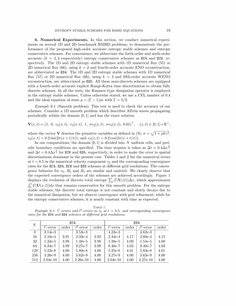
discretizations dominant in the present case. Tables 1 and 2 list the numerical errorsat t = 0.5 in the numerical velocity component v2 and the corresponding convergencerates for the EC4, ES4, EC6 and ES5 schemes at different grid resolutions. The conver-gence behavior for v3, B2 and B3 are similar and omitted. We clearly observe thatthe expected convergence orders of the schemes are achieved accordingly. Figure 1displays the evolution of discrete total entropy

∑i E(Ui(t))∆x, which approximates∫ 1

0E(U(x, t))dx that remains conservative for this smooth problem. For the entropy

stable schemes, the discrete total entropy is not constant and slowly decays due tothe numerical dissipation, but we observe convergence with grid refinement, while forthe entropy conservative schemes, it is nearly constant with time as expected.

Table 1Example 6.1: l1-errors and l2-errors in v2 at t = 0.5, and corresponding convergence

rates for the EC4 and ES4 schemes at different grid resolutions.

NEC4 ES4

l1-error order l2-error order l1-error order l2-error order8 3.14e-3 – 3.53e-3 – 4.23e-3 – 4.62e-3 –16 2.10e-4 3.91 2.33e-4 3.92 2.34e-4 4.17 2.60e-4 4.1532 1.33e-5 3.98 1.48e-5 3.98 1.38e-5 4.09 1.54e-5 4.0864 8.34e-7 3.99 9.27e-7 3.99 8.46e-7 4.03 9.40e-7 4.03128 5.22e-8 4.00 5.80e-8 4.00 5.25e-8 4.01 5.83e-8 4.01256 3.26e-9 4.00 3.62e-9 4.00 3.27e-9 4.00 3.63e-9 4.00512 2.04e-10 4.00 2.26e-10 4.00 2.04e-10 4.00 2.27e-10 4.00


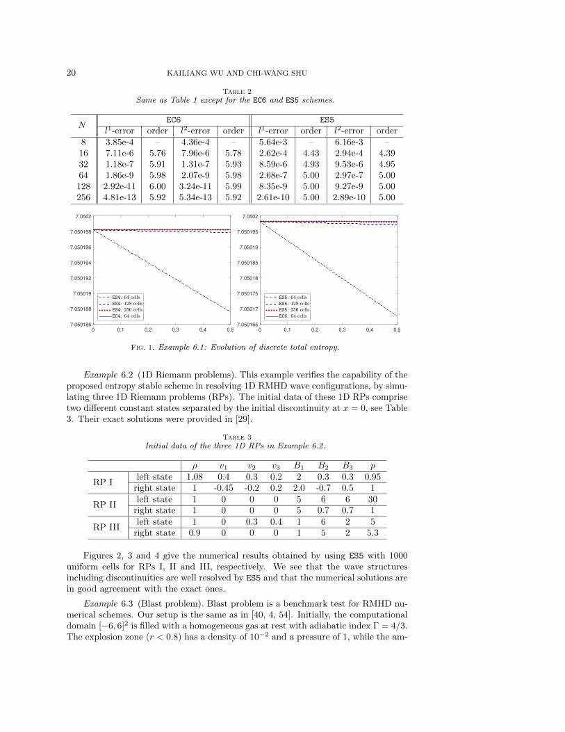
Table 2Same as Table 1 except for the EC6 and ES5 schemes.

NEC6 ES5

l1-error order l2-error order l1-error order l2-error order8 3.85e-4 – 4.36e-4 – 5.64e-3 – 6.16e-3 –16 7.11e-6 5.76 7.96e-6 5.78 2.62e-4 4.43 2.94e-4 4.3932 1.18e-7 5.91 1.31e-7 5.93 8.59e-6 4.93 9.53e-6 4.9564 1.86e-9 5.98 2.07e-9 5.98 2.68e-7 5.00 2.97e-7 5.00128 2.92e-11 6.00 3.24e-11 5.99 8.35e-9 5.00 9.27e-9 5.00256 4.81e-13 5.92 5.34e-13 5.92 2.61e-10 5.00 2.89e-10 5.00

0 0.1 0.2 0.3 0.4 0.5

7.050186

7.050188

7.05019

7.050192

7.050194

7.050196

7.050198

7.0502

0 0.1 0.2 0.3 0.4 0.5

7.050165

7.05017

7.050175

7.05018

7.050185

7.05019

7.050195

7.0502

Fig. 1. Example 6.1: Evolution of discrete total entropy.

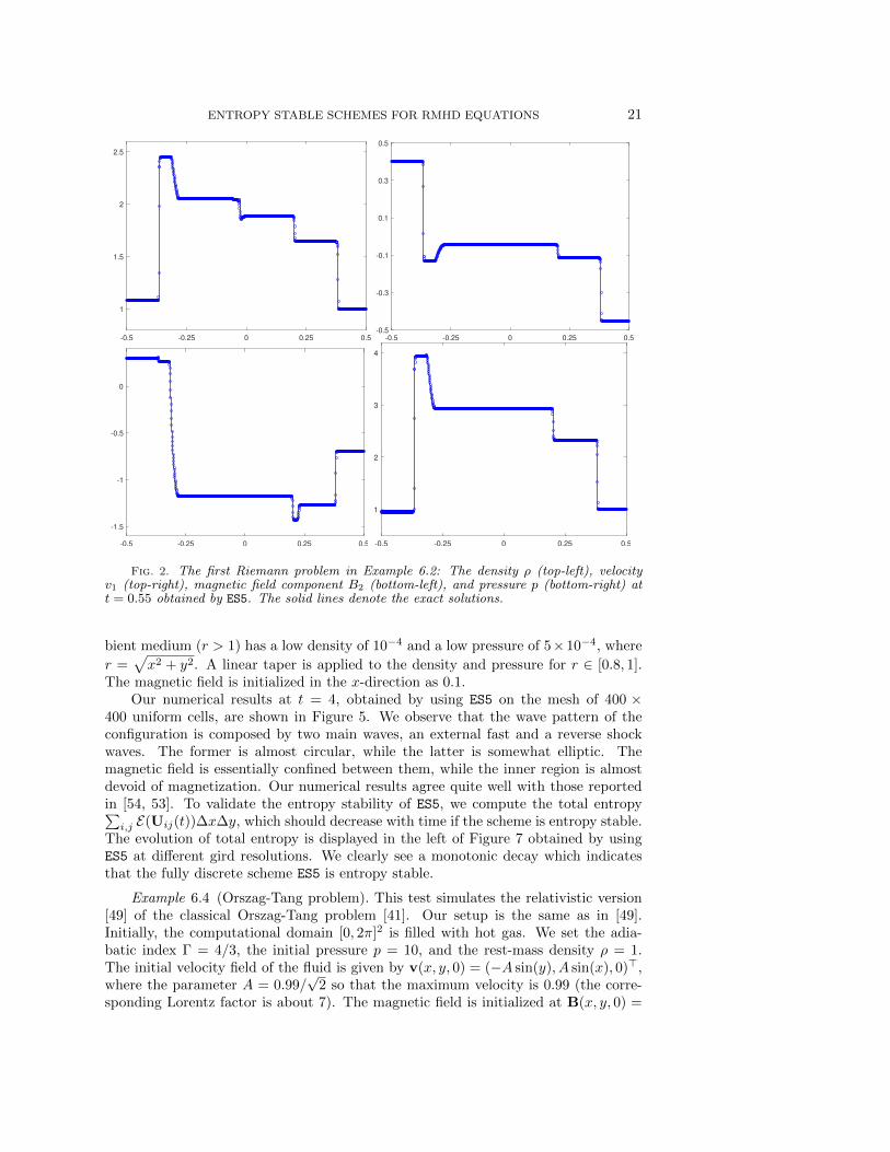
Example 6.2 (1D Riemann problems). This example verifies the capability of theproposed entropy stable scheme in resolving 1D RMHD wave configurations, by simu-lating three 1D Riemann problems (RPs). The initial data of these 1D RPs comprisetwo different constant states separated by the initial discontinuity at x = 0, see Table3. Their exact solutions were provided in [29].

Table 3Initial data of the three 1D RPs in Example 6.2.

ρ v1 v2 v3 B1 B2 B3 p

RP Ileft state 1.08 0.4 0.3 0.2 2 0.3 0.3 0.95

right state 1 -0.45 -0.2 0.2 2.0 -0.7 0.5 1

RP IIleft state 1 0 0 0 5 6 6 30

right state 1 0 0 0 5 0.7 0.7 1

RP IIIleft state 1 0 0.3 0.4 1 6 2 5

right state 0.9 0 0 0 1 5 2 5.3

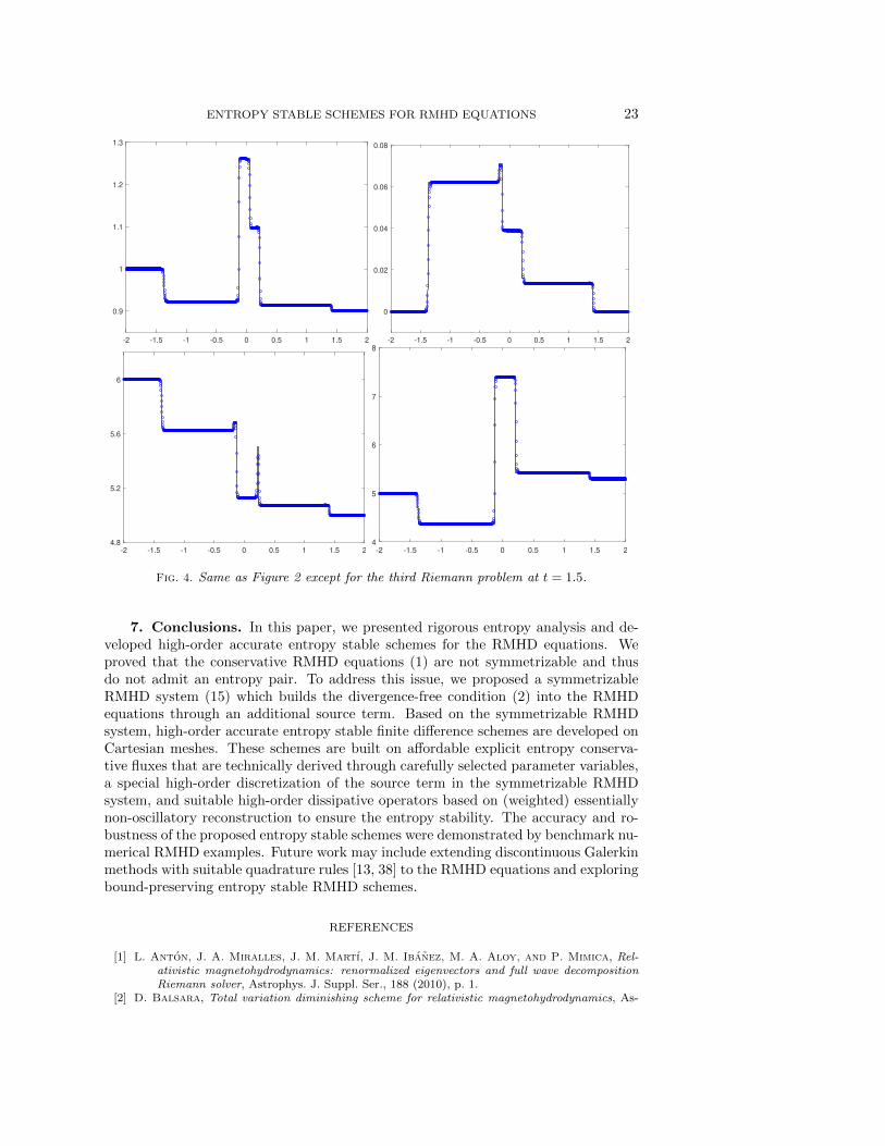
Figures 2, 3 and 4 give the numerical results obtained by using ES5 with 1000uniform cells for RPs I, II and III, respectively. We see that the wave structuresincluding discontinuities are well resolved by ES5 and that the numerical solutions arein good agreement with the exact ones.

Example 6.3 (Blast problem). Blast problem is a benchmark test for RMHD nu-merical schemes. Our setup is the same as in [40, 4, 54]. Initially, the computationaldomain [−6, 6]2 is filled with a homogeneous gas at rest with adiabatic index Γ = 4/3.The explosion zone (r < 0.8) has a density of 10−2 and a pressure of 1, while the am-


-0.5 -0.25 0 0.25 0.5

1

1.5

2

2.5

-0.5 -0.25 0 0.25 0.5

-0.5

-0.3

-0.1

0.1

0.3

0.5

-0.5 -0.25 0 0.25 0.5

-1.5

-1

-0.5

0

-0.5 -0.25 0 0.25 0.5

1

2

3

4

Fig. 2. The first Riemann problem in Example 6.2: The density ρ (top-left), velocityv1 (top-right), magnetic field component B2 (bottom-left), and pressure p (bottom-right) att = 0.55 obtained by ES5. The solid lines denote the exact solutions.

bient medium (r > 1) has a low density of 10−4 and a low pressure of 5×10−4, where

r =√x2 + y2. A linear taper is applied to the density and pressure for r ∈ [0.8, 1].

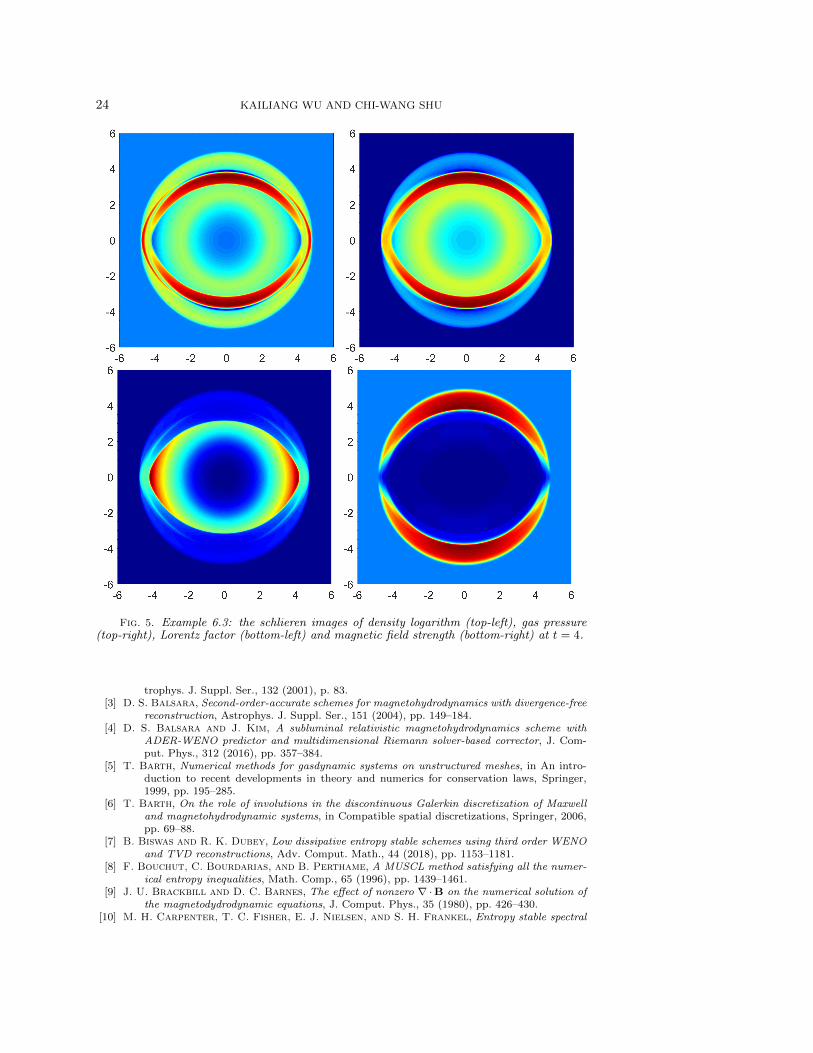
The magnetic field is initialized in the x-direction as 0.1.Our numerical results at t = 4, obtained by using ES5 on the mesh of 400 ×

400 uniform cells, are shown in Figure 5. We observe that the wave pattern of theconfiguration is composed by two main waves, an external fast and a reverse shockwaves. The former is almost circular, while the latter is somewhat elliptic. Themagnetic field is essentially confined between them, while the inner region is almostdevoid of magnetization. Our numerical results agree quite well with those reportedin [54, 53]. To validate the entropy stability of ES5, we compute the total entropy∑i,j E(Uij(t))∆x∆y, which should decrease with time if the scheme is entropy stable.

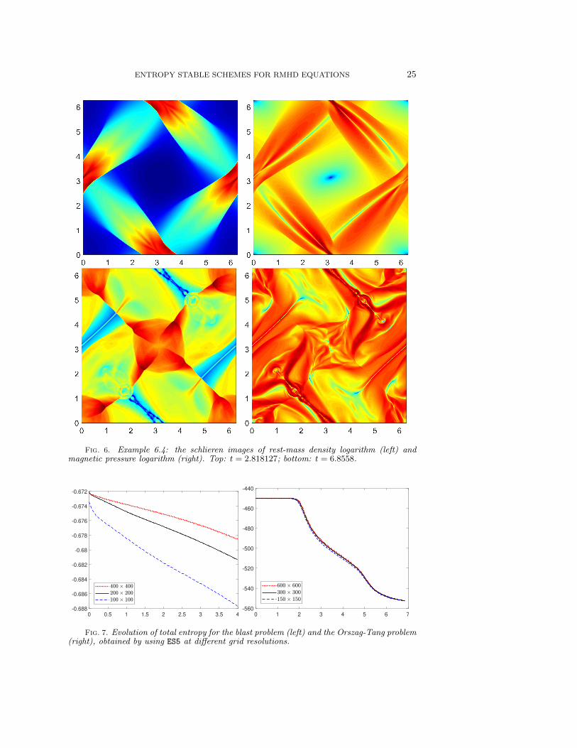
The evolution of total entropy is displayed in the left of Figure 7 obtained by usingES5 at different gird resolutions. We clearly see a monotonic decay which indicatesthat the fully discrete scheme ES5 is entropy stable.

Example 6.4 (Orszag-Tang problem). This test simulates the relativistic version[49] of the classical Orszag-Tang problem [41]. Our setup is the same as in [49].Initially, the computational domain [0, 2π]2 is filled with hot gas. We set the adia-batic index Γ = 4/3, the initial pressure p = 10, and the rest-mass density ρ = 1.The initial velocity field of the fluid is given by v(x, y, 0) = (−A sin(y), A sin(x), 0)>,where the parameter A = 0.99/

√2 so that the maximum velocity is 0.99 (the corre-

sponding Lorentz factor is about 7). The magnetic field is initialized at B(x, y, 0) =


-0.5 -0.25 0 0.25 0.5

0

0.5

1

1.5

2

2.5

3

3.5

-0.5 -0.25 0 0.25 0.5

-0.2

0

0.2

0.4

0.6

0.8

-0.5 -0.25 0 0.25 0.5

0

1

2

3

4

5

6

7

-0.5 -0.25 0 0.25 0.5

0

5

10

15

20

25

30

35

Fig. 3. Same as Figure 2 except for the second Riemann problem at t = 0.4.

(− sin y, sin(2x), 0)>. Periodic conditions are specified at all the boundaries. Al-though the solution of this problem is smooth initially, complicated wave structuresare formed as the time increases, and turbulence behavior will be produced eventually.

Figure 6 gives the numerical results obtained by using ES5 on 600× 600 uniformgrids. In comparison with the results in [49], the complicated flow structures are wellcaptured by ES5 with high resolution. To validate the entropy stability, the evolutionof total entropy is shown in the right of Figure 7 obtained by using ES5 at differentgird resolutions. We observe that the total entropy remains constant at initial timesbecause initially the solution is smooth, and it starts to decrease at t ≈ 2 whendiscontinuities start to form, as expected.

Example 6.5 (Shock cloud interaction problem). This problem describes the dis-ruption of a high density cloud by a strong shock wave. Our setup is the sameas in [31]. The computational domain is [−0.2, 1.2] × [0, 1], with the left bound-ary specified as inflow condition and the others as outflow conditions. Initially, ashock wave moves to the right from x = 0.05, with the left and right states VL =(3.86859, 0.68, 0, 0, 0, 0.84981,−0.84981, 1.25115)> and VR = (1, 0, 0, 0, 0, 0.16106, 0.16106, 0.05)>,respectively. There exists a rest circular cloud centred at the point (0.25, 0.5) withradius 0.15. The cloud has the same states to the surrounding fluid except for a higherdensity of 30. Figure 8 displays the schlieren images of rest-mass density logarithmand magnetic pressure logarithm at t = 1.2 obtained by using ES5 with 560 × 400uniform cells. One can see that the discontinuities are captured with high resolution,and the results agree well with those in [31, 55, 53].


-2 -1.5 -1 -0.5 0 0.5 1 1.5 2

0.9

1

1.1

1.2

1.3

-2 -1.5 -1 -0.5 0 0.5 1 1.5 2

0

0.02

0.04

0.06

0.08

-2 -1.5 -1 -0.5 0 0.5 1 1.5 2

4.8

5.2

5.6

6

-2 -1.5 -1 -0.5 0 0.5 1 1.5 2

4

5

6

7

8

Fig. 4. Same as Figure 2 except for the third Riemann problem at t = 1.5.

7. Conclusions. In this paper, we presented rigorous entropy analysis and de-veloped high-order accurate entropy stable schemes for the RMHD equations. Weproved that the conservative RMHD equations (1) are not symmetrizable and thusdo not admit an entropy pair. To address this issue, we proposed a symmetrizableRMHD system (15) which builds the divergence-free condition (2) into the RMHDequations through an additional source term. Based on the symmetrizable RMHDsystem, high-order accurate entropy stable finite difference schemes are developed onCartesian meshes. These schemes are built on affordable explicit entropy conserva-tive fluxes that are technically derived through carefully selected parameter variables,a special high-order discretization of the source term in the symmetrizable RMHDsystem, and suitable high-order dissipative operators based on (weighted) essentiallynon-oscillatory reconstruction to ensure the entropy stability. The accuracy and ro-bustness of the proposed entropy stable schemes were demonstrated by benchmark nu-merical RMHD examples. Future work may include extending discontinuous Galerkinmethods with suitable quadrature rules [13, 38] to the RMHD equations and exploringbound-preserving entropy stable RMHD schemes.

REFERENCES

[1] L. Anton, J. A. Miralles, J. M. Martı, J. M. Ibanez, M. A. Aloy, and P. Mimica, Rel-ativistic magnetohydrodynamics: renormalized eigenvectors and full wave decompositionRiemann solver, Astrophys. J. Suppl. Ser., 188 (2010), p. 1.

[2] D. Balsara, Total variation diminishing scheme for relativistic magnetohydrodynamics, As-


Fig. 5. Example 6.3: the schlieren images of density logarithm (top-left), gas pressure(top-right), Lorentz factor (bottom-left) and magnetic field strength (bottom-right) at t = 4.

trophys. J. Suppl. Ser., 132 (2001), p. 83.[3] D. S. Balsara, Second-order-accurate schemes for magnetohydrodynamics with divergence-free

reconstruction, Astrophys. J. Suppl. Ser., 151 (2004), pp. 149–184.[4] D. S. Balsara and J. Kim, A subluminal relativistic magnetohydrodynamics scheme with

ADER-WENO predictor and multidimensional Riemann solver-based corrector, J. Com-put. Phys., 312 (2016), pp. 357–384.

[5] T. Barth, Numerical methods for gasdynamic systems on unstructured meshes, in An intro-duction to recent developments in theory and numerics for conservation laws, Springer,1999, pp. 195–285.

[6] T. Barth, On the role of involutions in the discontinuous Galerkin discretization of Maxwelland magnetohydrodynamic systems, in Compatible spatial discretizations, Springer, 2006,pp. 69–88.

[7] B. Biswas and R. K. Dubey, Low dissipative entropy stable schemes using third order WENOand TVD reconstructions, Adv. Comput. Math., 44 (2018), pp. 1153–1181.

[8] F. Bouchut, C. Bourdarias, and B. Perthame, A MUSCL method satisfying all the numer-ical entropy inequalities, Math. Comp., 65 (1996), pp. 1439–1461.

[9] J. U. Brackbill and D. C. Barnes, The effect of nonzero ∇ ·B on the numerical solution ofthe magnetodydrodynamic equations, J. Comput. Phys., 35 (1980), pp. 426–430.

[10] M. H. Carpenter, T. C. Fisher, E. J. Nielsen, and S. H. Frankel, Entropy stable spectral


Fig. 6. Example 6.4: the schlieren images of rest-mass density logarithm (left) andmagnetic pressure logarithm (right). Top: t = 2.818127; bottom: t = 6.8558.

0 0.5 1 1.5 2 2.5 3 3.5 4

-0.688

-0.686

-0.684

-0.682

-0.68

-0.678

-0.676

-0.674

-0.672

0 1 2 3 4 5 6 7

-560

-540

-520

-500

-480

-460

-440

Fig. 7. Evolution of total entropy for the blast problem (left) and the Orszag-Tang problem(right), obtained by using ES5 at different grid resolutions.


Fig. 8. Example 6.5: the schlieren images of rest-mass density logarithm (left) andmagnetic pressure logarithm (right) at time t = 1.2.

collocation schemes for the Navier–Stokes equations: Discontinuous interfaces, SIAM J.Sci. Comput., 36 (2014), pp. B835–B867.

[11] P. Chandrashekar, Kinetic energy preserving and entropy stable finite volume schemes forcompressible Euler and Navier-Stokes equations, Commun. Comput. Phys., 14 (2013),pp. 1252–1286.

[12] P. Chandrashekar and C. Klingenberg, Entropy stable finite volume scheme for ideal com-pressible MHD on 2-D Cartesian meshes, SIAM J. Numer. Anal., 54 (2016), pp. 1313–1340.

[13] T. Chen and C.-W. Shu, Entropy stable high order discontinuous Galerkin methods withsuitable quadrature rules for hyperbolic conservation laws, J. Comput. Phys., 345 (2017),pp. 427–461.

[14] M. G. Crandall and A. Majda, Monotone difference approximations for scalar conservationlaws, Math. Comp., 34 (1980), pp. 1–21.

[15] A. Dedner, F. Kemm, D. Kroner, C.-D. Munz, T. Schnitzer, and M. Wesenberg, Hyper-bolic divergence cleaning for the MHD equations, J. Comput. Phys., 175 (2002), pp. 645–673.

[16] D. Derigs, A. R. Winters, G. J. Gassner, and S. Walch, A novel high-order, entropy stable,3D AMR MHD solver with guaranteed positive pressure, J. Comput. Phys., 317 (2016),pp. 223–256.

[17] D. Derigs, A. R. Winters, G. J. Gassner, S. Walch, and M. Bohm, Ideal GLM-MHD:About the entropy consistent nine-wave magnetic field divergence diminishing ideal mag-netohydrodynamics equations, J. Comput. Phys., 364 (2018), pp. 420–467.

[18] J. Duan and H. Tang, High-order accurate entropy stable finite difference schemes for one-andtwo-dimensional special relativistic hydrodynamics, arXiv:1905.06092, (2019).

[19] C. R. Evans and J. F. Hawley, Simulation of magnetohydrodynamic flows: a constrainedtransport method, Astrophys. J., 332 (1988), pp. 659–677.

[20] T. C. Fisher and M. H. Carpenter, High-order entropy stable finite difference schemes fornonlinear conservation laws: Finite domains, J. Comput. Phys., 252 (2013), pp. 518–557.

[21] U. S. Fjordholm, S. Mishra, and E. Tadmor, Arbitrarily high-order accurate entropy sta-ble essentially nonoscillatory schemes for systems of conservation laws, SIAM J. Numer.Anal., 50 (2012), pp. 544–573.

[22] U. S. Fjordholm, S. Mishra, and E. Tadmor, ENO reconstruction and ENO interpolationare stable, Found. Comput. Math., 13 (2013), pp. 139–159.

[23] U. S. Fjordholm and D. Ray, A sign preserving WENO reconstruction method, J. Sci. Com-put., 68 (2016), pp. 42–63.

[24] G. J. Gassner, A skew-symmetric discontinuous Galerkin spectral element discretization andits relation to SBP-SAT finite difference methods, SIAM J. Sci. Comput., 35 (2013),pp. A1233–A1253.

[25] G. J. Gassner, A. R. Winters, and D. A. Kopriva, A well balanced and entropy conservativediscontinuous Galerkin spectral element method for the shallow water equations, Appl.Math. Comput., 272 (2016), pp. 291–308.

[26] E. Godlewski and P.-A. Raviart, Numerical approximation of hyperbolic systems of conser-vation laws, vol. 118, Springer Science & Business Media, 2013.

[27] S. K. Godunov, Symmetric form of the equations of magnetohydrodynamics, Numerical Meth-


ods for Mechanics of Continuum Medium, 1 (1972), pp. 26–34.[28] F. Guercilena, D. Radice, and L. Rezzolla, Entropy-limited hydrodynamics: a novel ap-

proach to relativistic hydrodynamics, Comput. Astrophys. Cosmol., 4 (2017), p. 3.[29] F. Guercilena and L. Rezzolla, The exact solution of the Riemann problem in relativistic

magnetohydrodynamics, J. Fluid Mech., 562 (2006), pp. 223–259.[30] A. Harten, J. M. Hyman, P. D. Lax, and B. Keyfitz, On finite-difference approximations

and entropy conditions for shocks, Commun. Pure Appl. Math., 29 (1976), pp. 297–322.[31] P. He and H. Tang, An adaptive moving mesh method for two-dimensional relativistic mag-

netohydrodynamics, Comput. Fluids, 60 (2012), pp. 1–20.[32] J. S. Hesthaven and F. Monkeberg, Entropy stable essentially nonoscillatory methods based

on RBF reconstruction, ESAIM. Math. Model Numer. Anal., 53 (2019), pp. 925–958.[33] A. Hiltebrand and S. Mishra, Entropy stable shock capturing space–time discontinuous

galerkin schemes for systems of conservation laws, Numer. Math., 126 (2014), pp. 103–151.[34] F. Ismail and P. L. Roe, Affordable, entropy-consistent Euler flux functions II: Entropy

production at shocks, J. Comput. Phys., 228 (2009), pp. 5410–5436.[35] P. G. Lefloch, J.-M. Mercier, and C. Rohde, Fully discrete, entropy conservative schemes

of arbitrary order, SIAM J. Numer. Anal., 40 (2002), pp. 1968–1992.[36] F. Li and C.-W. Shu, Locally divergence-free discontinuous Galerkin methods for MHD equa-

tions, J. Sci. Comput., 22 (2005), pp. 413–442.[37] F. Li, L. Xu, and S. Yakovlev, Central discontinuous Galerkin methods for ideal MHD

equations with the exactly divergence-free magnetic field, J. Comput. Phys., 230 (2011),pp. 4828–4847.

[38] Y. Liu, C.-W. Shu, and M. Zhang, Entropy stable high order discontinuous Galerkin methodsfor ideal compressible MHD on structured meshes, J. Comput. Phys., 354 (2018), pp. 163–178.

[39] J. M. Martı and E. Muller, Grid-based methods in relativistic hydrodynamics and magne-tohydrodynamics, Living Rev. Comput. Astrophys., 1 (2015), p. 3.

[40] A. Mignone and G. Bodo, An HLLC riemann solver for relativistic flows–II. magnetohydro-dynamics, Mon. Not. R. Astron. Soc., 368 (2006), pp. 1040–1054.

[41] S. A. Orszag and C.-M. Tang, Small-scale structure of two-dimensional magnetohydrody-namic turbulence, J. Fluid Mech., 90 (1979), pp. 129–143.

[42] S. Osher, Riemann solvers, the entropy condition, and difference, SIAM J. Numer. Anal., 21(1984), pp. 217–235.

[43] S. Osher and E. Tadmor, On the convergence of difference approximations to scalar conser-vation laws, Math. Comp., 50 (1988), pp. 19–51.

[44] K. G. Powell, P. Roe, R. Myong, and T. Gombosi, An upwind scheme for magnetohydro-dynamics, in 12th Computational Fluid Dynamics Conference, 1995, p. 1704.

[45] H. Ranocha, Comparison of some entropy conservative numerical fluxes for the euler equa-tions, J. Sci. Comput., 76 (2018), pp. 216–242.

[46] E. Tadmor, The numerical viscosity of entropy stable schemes for systems of conservationlaws. I, Math. Comp., 49 (1987), pp. 91–103.

[47] E. Tadmor, Entropy stability theory for difference approximations of nonlinear conservationlaws and related time-dependent problems, Acta Numer., 12 (2003), pp. 451–512.

[48] G. Toth, The ∇ ·B = 0 constraint in shock-capturing magnetohydrodynamics codes, J. Com-put. Phys., 161 (2000), pp. 605–652.

[49] B. van der Holst, R. Keppens, and Z. Meliani, A multidimensional grid-adaptive relativisticmagnetofluid code, Comput. Phys. Commun., 179 (2008), pp. 617–627.

[50] A. R. Winters and G. J. Gassner, Affordable, entropy conserving and entropy stable fluxfunctions for the ideal MHD equations, J. Comput. Phys., 304 (2016), pp. 72–108.

[51] K. Wu, Positivity-preserving analysis of numerical schemes for ideal magnetohydrodynamics,SIAM J. Numer. Anal., 56 (2018), pp. 2124–2147.

[52] K. Wu and C.-W. Shu, A provably positive discontinuous Galerkin method for multidimen-sional ideal magnetohydrodynamics, SIAM J. Sci. Comput., 40 (2018), pp. B1302–B1329.

[53] K. Wu and H. Tang, Admissible states and physical-constraints-preserving schemes for rel-ativistic magnetohydrodynamic equations, Math. Models Methods Appl. Sci., 27 (2017),pp. 1871–1928.

[54] O. Zanotti, F. Fambri, and M. Dumbser, Solving the relativistic magnetohydrodynamicsequations with ADER discontinuous Galerkin methods, a posteriori subcell limiting andadaptive mesh refinement, Mon. Not. R. Astron. Soc., 452 (2015), pp. 3010–3029.

[55] J. Zhao and H. Tang, Runge-Kutta discontinuous Galerkin methods for the special relativisticmagnetohydrodynamics, J. Comput. Phys., 343 (2017), pp. 33–72.

Documents

Entropy Stable Schemes for RMHD - math.umd.edu